Abstract

A detailed study of the heavy quark $h=c,b,\ldots$ contributions to deeply virtual Compton scattering is performed at both the amplitude and the cross section level, and their phenomenological relevance is discussed. For this purpose I calculate the lowest order off-forward photon-gluon scattering amplitude with a massive quark loop and the corresponding hard scattering coefficients. In a first numerical analysis these fixed order perturbation theory results are compared with the conventional intrinsic “massless” parton approach considering generalized parton distributions for the heavy quarks. The differences between these two prescriptions can be quite significant, especially at small skewedness where the massless approach largely overestimates the deeply virtual Compton scattering cross section.

1 Introduction

In deeply virtual Compton scattering (DVCS) [1, 2, 3] a highly virtual photon, generally radiated from a charged high-energy lepton, converts to a real photon by scattering on a nucleon target that remains intact. The phenomenology of DVCS looks very promising with first data in different kinematic regions being available from several groups at fixed target [4, 5] and collider experiments [6, 7]. On the theoretical side the amount of uncertainties in the predictions for DVCS could be reduced by incorporating next-to-leading order corrections in perturbative quantum chromodynamics (QCD) [8, 9, 10] and power corrections to the leading twist-two results starting at the twist-three level [11, 12, 13].

The main motivation for studying DVCS is the access to new non-perturbative information on the structure of the nucleon carried by generalized parton distributions (GPDs) [14, 1, 2, 15, 3, 16], which will deliver insight into the spin structure of the nucleon, in particular the quark and gluon spin and orbital angular momentum contributions, [1] and into the nucleon structure in three dimensions [17]. An excellent survey of the theory of GPDs and their experimental accessibility can be found in a recent comprehensive report [18].

It is reasonable to inspect the inclusive proton structure function $F_{2}$ in deep inelastic scattering (DIS) due to its close connection to the general Compton amplitude via the optical theorem. In the kinematic region relevant for DVCS at the collider experiments the charm contribution $F_{2}^{c}$ to the proton structure function has been found to be up to $20\%$ [19, 20]. If one presumes this same ratio for the corresponding form factor of the DVCS amplitude this results in a charm contribution of about one third to the DVCS cross section (amplitude squared). Hence a proper treatment of charm in DVCS can be quite important.

Generally, heavy quarks $h=c,b,t$ are characterized by $m_{h}^{2}\gg\varLambda_{\text{QCD}}^{2}$ whereas light (“massless”) quarks have $m_{u,d,s}^{2}\ll\varLambda_{\text{QCD}}^{2}$. In fixed order (FO) perturbation theory, heavy quarks contribute in lowest order to the photon-gluon scattering (PGS) $\gamma^{\ast}g\to\gamma{}g$ DVCS subprocess where they appear as massive internal fermion lines. As is well known, such a fixed order calculation correctly describes the threshold region $\hat{s}\gtrsim 4m_{h}^{2}$ in DIS [19, 20, 21, 22], and its perturbative stability has been demonstrated in Ref. [23] even up to $\hat{s}\sim 10^{6}\,\text{GeV}^{2}$. In the conventional parton model approach potentially large logarithms $\log^{n}(m_{h}^{2}/\hat{s})$ appearing in the fixed order PGS result are resummed to all orders and absorbed into intrinsic “massless” parton (MP) distributions for the heavy flavors [24].

In the next section, after giving a rough overview of DVCS in the leading twist approximation, the technicalities of incorporating heavy quark contributions in the DVCS amplitude are described and the need for massive hard scattering coefficient functions is explained. In Sec. 3 a systematic way to calculate the lowest-order of PGS with a massive quark loop is introduced whose relevant results are presented in Sec. 4. This completes the requisites for a first numerical analysis of heavy quark effects in DVCS where the numerical results at the amplitude as well as at the cross section level are discussed in Sec. 5. Finally, in Sec. 6 the conclusions are drawn and an outlook is given.

2 Leading twist DVCS amplitude

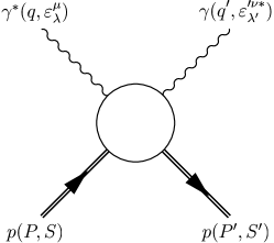
First, some general properties of DVCS have to be reiterated where mainly the notations of Refs. [25, 8] are used. The general kinematics of DVCS on a proton are shown in Fig. 1

Figure 1: General kinematics of deeply virtual Compton scattering on a proton.

with the masses defined to be $Q^{2}:=-q^{2}$ and $M^{2}:={}P^{2}=P^{\prime 2}$. An independent set of momenta is given by

$$\text{$P$\makebox[6.80557pt]{\hskip 0.86108pt$\overline{\phantom{\mathrm{P}}}$}}\vphantom{P}:=(P+P^{\prime})/2\;,\quad\text{$q$\makebox[5.27779pt]{\hskip 0.86108pt$\overline{\phantom{\mathrm{q}}}$}}\vphantom{q}:=(q+q^{\prime})/2\;,\quad\varDelta:=P^{\prime}-P$$ (1)

that leads to the following five Lorentz invariants

$$\text{$Q$\makebox[7.7778pt]{\hskip 0.86108pt$\overline{\phantom{\mathrm{Q}}}$}}\vphantom{Q}^{2}:=-\text{$q$\makebox[5.27779pt]{\hskip 0.86108pt$\overline{\phantom{\mathrm{q}}}$}}\vphantom{q}^{2}\;,\quad x:=\frac{\text{$Q$\makebox[7.7778pt]{\hskip 0.86108pt$\overline{\phantom{\mathrm{Q}}}$}}\vphantom{Q}^{2}}{2{\text{$P$\makebox[6.80557pt]{\hskip 0.86108pt$\overline{\phantom{\mathrm{P}}}$}}\vphantom{P}}{\cdot}{\text{$q$\makebox[5.27779pt]{\hskip 0.86108pt$\overline{\phantom{\mathrm{q}}}$}}\vphantom{q}}}\;,\quad\xi:=-\frac{{\varDelta}{\cdot}{\text{$q$\makebox[5.27779pt]{\hskip 0.86108pt$\overline{\phantom{\mathrm{q}}}$}}\vphantom{q}}}{2{\text{$P$\makebox[6.80557pt]{\hskip 0.86108pt$\overline{\phantom{\mathrm{P}}}$}}\vphantom{P}}{\cdot}{\text{$q$\makebox[5.27779pt]{\hskip 0.86108pt$\overline{\phantom{\mathrm{q}}}$}}\vphantom{q}}}\;,\quad t:=\varDelta^{2}\;,\quad\text{$M$\makebox[9.16669pt]{\hskip 0.86108pt$\overline{\phantom{\mathrm{M}}}$}}\vphantom{M}^{2}:=\text{$P$\makebox[6.80557pt]{\hskip 0.86108pt$\overline{\phantom{\mathrm{P}}}$}}\vphantom{P}^{2}=M^{2}-t/4$$ (2)

where for the moment the outgoing photon is also considered virtual. Only the first three invariants survive the generalized Bjorken limit $\text{$Q$\makebox[7.7778pt]{\hskip 0.86108pt$\overline{\phantom{\mathrm{Q}}}$}}\vphantom{Q}^{2}\to\infty$ with $x,\xi$ fixed in which the first two are straightforward generalizations of corresponding invariants in DIS. The additional scaling variable $\xi$, the so-called skewedness, is a measure of the difference between the two photon virtualities. Furthermore, the following invariants prove to be helpful for the representation of the analytical results in Sec. 4

$$\hat{s}:=(\text{$P$\makebox[6.80557pt]{\hskip 0.86108pt$\overline{\phantom{\mathrm{P}}}$}}\vphantom{P}+\text{$q$\makebox[5.27779pt]{\hskip 0.86108pt$\overline{\phantom{\mathrm{q}}}$}}\vphantom{q})^{2}=\text{$Q$\makebox[7.7778pt]{\hskip 0.86108pt$\overline{\phantom{\mathrm{Q}}}$}}\vphantom{Q}^{2}(-1+1/x)+\text{$M$\makebox[9.16669pt]{\hskip 0.86108pt$\overline{\phantom{\mathrm{M}}}$}}\vphantom{M}^{2}\;,\quad\hat{u}:=(\text{$P$\makebox[6.80557pt]{\hskip 0.86108pt$\overline{\phantom{\mathrm{P}}}$}}\vphantom{P}-\text{$q$\makebox[5.27779pt]{\hskip 0.86108pt$\overline{\phantom{\mathrm{q}}}$}}\vphantom{q})^{2}=\text{$Q$\makebox[7.7778pt]{\hskip 0.86108pt$\overline{\phantom{\mathrm{Q}}}$}}\vphantom{Q}^{2}(-1-1/x)+\text{$M$\makebox[9.16669pt]{\hskip 0.86108pt$\overline{\phantom{\mathrm{M}}}$}}\vphantom{M}^{2}\;,$$

$$q^{2}=(\text{$q$\makebox[5.27779pt]{\hskip 0.86108pt$\overline{\phantom{\mathrm{q}}}$}}\vphantom{q}+\varDelta/2)^{2}=\text{$Q$\makebox[7.7778pt]{\hskip 0.86108pt$\overline{\phantom{\mathrm{Q}}}$}}\vphantom{Q}^{2}(-1-\xi/x)+t/4\;,\quad q^{\prime 2}=(\text{$q$\makebox[5.27779pt]{\hskip 0.86108pt$\overline{\phantom{\mathrm{q}}}$}}\vphantom{q}-\varDelta/2)^{2}=\text{$Q$\makebox[7.7778pt]{\hskip 0.86108pt$\overline{\phantom{\mathrm{Q}}}$}}\vphantom{Q}^{2}(-1+\xi/x)+t/4$$ (3)

where $\text{$M$\makebox[9.16669pt]{\hskip 0.86108pt$\overline{\phantom{\mathrm{M}}}$}}\vphantom{M}^{2}$ and $t/4$ are neglected in the generalized Bjorken limit. In DVCS with a real photon in the final state only one scaling variable remains

$$x\approx\xi=x(1-t/4\text{$Q$\makebox[7.7778pt]{\hskip 0.86108pt$\overline{\phantom{\mathrm{Q}}}$}}\vphantom{Q}^{2})\;,\quad\text{$Q$\makebox[7.7778pt]{\hskip 0.86108pt$\overline{\phantom{\mathrm{Q}}}$}}\vphantom{Q}^{2}=Q^{2}/2+t/4\approx{}Q^{2}/2\;,$$ (4)

which is chosen to be $\xi$ to avoid confusion with the usual Bjorken variable $x_{B}\approx 2\xi/(1+\xi)$ in DIS, and it is more appropriate to use $Q^{2}$.

The dynamics is contained in the DVCS amplitude

$$-i\mathop{T^{\nu\mu}}=\int{e^{i{\text{$q$\makebox[3.69444pt]{\hskip 0.60275pt$\overline{\phantom{\mathrm{q}}}$}}\vphantom{q}}{\cdot}{z}}\langle{P^{\prime}S^{\prime}}\lvert{\mathcal{T}\left[{J^{\nu}(z/2)J^{\mu}(-z/2)}\right]}\rvert{PS}\rangle}\mathop{\mathrm{d}^{4}{z}}$$ (5)

that is given by the time-ordered product of two currents which are related to the electromagnetic current by $J_{\text{em}}^{\mu}(z)=eJ^{\mu}(z)$. The leading twist contributions, apart from those that arise due to photon helicity flip which are beyond the scope of this work, are contained in the following two, transversal photon spin conserving, form factors

$$\mathop{T^{\nu\mu}}=\sum_{\lambda=\pm}\varepsilon^{\prime\nu\vphantom{\mu}}_{\lambda}\varepsilon_{\lambda}^{\mu\ast\vphantom{\mu}}\mathop{T_{\text{T}}}+\sum_{\lambda=\pm}\lambda\varepsilon^{\prime\nu\vphantom{\mu}}_{\lambda}\varepsilon_{\lambda}^{\mu\ast\vphantom{\mu}}\mathop{\widetilde{T}_{\text{T}}}+\ldots$$ (6)

whose exact Lorentz structures will be defined when they are explicitly needed in the next section. For now it is sufficient to note that they are equivalent to the usual ones in the generalized Bjorken limit, e. g. the tensors $\tilde{t}_{\mu\nu}$ {Eq. (9) in Ref.[8]}. These two form factors can be further decomposed with respect to their Dirac structure

$$\mathop{T_{\text{T}}} =\text{$U$\makebox[7.50002pt]{\hskip 0.86108pt$\overline{\phantom{\mathrm{U}}}$}}(P^{\prime},S^{\prime})\left[\mathop{T_{\text{T},1}}(\xi,t,Q^{2})\frac{\text{$\text{$q$\makebox[5.27779pt]{\hskip 0.86108pt$\overline{\phantom{\mathrm{q}}}$}}\vphantom{q}$\makebox[14.9236pt]{/}}}{2{\text{$P$\makebox[6.80557pt]{\hskip 0.86108pt$\overline{\phantom{\mathrm{P}}}$}}\vphantom{P}}{\cdot}{\text{$q$\makebox[5.27779pt]{\hskip 0.86108pt$\overline{\phantom{\mathrm{q}}}$}}\vphantom{q}}}+\mathop{T_{\text{T},2}}(\xi,t,Q^{2})\frac{i\sigma^{\mu\nu}\text{$q$\makebox[5.27779pt]{\hskip 0.86108pt$\overline{\phantom{\mathrm{q}}}$}}\vphantom{q}_{\mu}\varDelta_{\nu}}{4M{\text{$P$\makebox[6.80557pt]{\hskip 0.86108pt$\overline{\phantom{\mathrm{P}}}$}}\vphantom{P}}{\cdot}{\text{$q$\makebox[5.27779pt]{\hskip 0.86108pt$\overline{\phantom{\mathrm{q}}}$}}\vphantom{q}}}\right]U(P,S)\;,$$ (7)

$$\mathop{\widetilde{T}_{\text{T}}} =\text{$U$\makebox[7.50002pt]{\hskip 0.86108pt$\overline{\phantom{\mathrm{U}}}$}}(P^{\prime},S^{\prime})\left[\mathop{\widetilde{T}_{\text{T},\text{A}}}(\xi,t,Q^{2})\frac{\text{$\text{$q$\makebox[5.27779pt]{\hskip 0.86108pt$\overline{\phantom{\mathrm{q}}}$}}\vphantom{q}$\makebox[14.9236pt]{/}}}{2{\text{$P$\makebox[6.80557pt]{\hskip 0.86108pt$\overline{\phantom{\mathrm{P}}}$}}\vphantom{P}}{\cdot}{\text{$q$\makebox[5.27779pt]{\hskip 0.86108pt$\overline{\phantom{\mathrm{q}}}$}}\vphantom{q}}}+\mathop{\widetilde{T}_{\text{T},\text{P}}}(\xi,t,Q^{2})\frac{{\text{$q$\makebox[5.27779pt]{\hskip 0.86108pt$\overline{\phantom{\mathrm{q}}}$}}\vphantom{q}}{\cdot}{\varDelta}}{4M{\text{$P$\makebox[6.80557pt]{\hskip 0.86108pt$\overline{\phantom{\mathrm{P}}}$}}\vphantom{P}}{\cdot}{\text{$q$\makebox[5.27779pt]{\hskip 0.86108pt$\overline{\phantom{\mathrm{q}}}$}}\vphantom{q}}}\right]\gamma_{5}U(P,S)$$ (8)

in analogy to the form factors of the electromagnetic current between two nucleon states.

On the basis of the factorization theorems proven in Refs. [26, 25, 27] each of these form factors can be expressed as convolutions of GPDs with perturbatively calculable hard scattering coefficients such as

$$\mathop{T_{\text{T}}}=\sum_{a=q,g}\int_{-1}^{+1}\frac{\mathop{\mathrm{d}{y}}}{y}\mathop{f_{a}}(y,\xi,t,\mu)\sum_{b=q^{\prime}}e_{b}^{2}\mathop{t_{\text{T},ba}}(\xi/y,Q^{2},\mu)\;.$$ (9)

Equivalent formulas can be obtained after the replacements $\mathop{T_{\text{T}}}\to\mathop{T_{\text{T},1}},\mathop{T_{\text{T},2}}$ and $\mathop{f_{a}}\to\mathop{H_{a}},\mathop{E_{a}}$, or $\mathop{T_{\text{T}}}\to\mathop{\widetilde{T}_{\text{T}}},\mathop{\widetilde{T}_{\text{T},\text{A}}},\mathop{\widetilde{T}_{\text{T},\text{P}}}$, $\mathop{f_{a}}\to\mathop{\tilde{f}_{a}},\mathop{\widetilde{H}_{a}},\mathop{\widetilde{E}_{a}}$, and $\mathop{t_{\text{T},ba}}\to\mathop{\tilde{t}_{\text{T},ba}}$. The GPDs in Eq. (9) are defined in such a way that they have the closest possible connection to the unpolarized and polarized DIS parton distribution functions, that is $\mathop{H_{q,g}}(x,0,0,\mu)\equiv{}q,g(x,\mu)$ and $\mathop{\widetilde{H}_{q,g}}(x,0,0,\mu)\equiv{}\delta{}q,\delta{}g(x,\mu)$, respectively. The factorization scale $\mu$ is as usual assumed to be equal to the renormalization scale with the common choice $\mu^{2}=Q^{2}$. The hard scattering coefficients describe the scattering process $\gamma^{\ast}a\to\gamma{}a$ of the intrinsic parton $a$ with the coupling to the photon being mediated by the quark $b$ and accordingly define the sums in the factorization theorems.

Crossing symmetry of the Compton amplitude allows to rewrite the hard scattering coefficients in the following form

$$\mathop{t_{\text{T},ba}}(z,Q^{2},\mu) =\mathop{C_{\text{T},ba}}(z,Q^{2},\mu)+\mathop{C_{\text{T},ba}}(-z,Q^{2},\mu)\;,$$

$$\mathop{\tilde{t}_{\text{T},ba}}(z,Q^{2},\mu) =\mathop{\widetilde{C}_{\text{T},ba}}(z,Q^{2},\mu)-\mathop{\widetilde{C}_{\text{T},ba}}(-z,Q^{2},\mu)$$ (10)

where the definition of the coefficient function $\mathop{C_{\text{T},ba}}$ ($\mathop{\widetilde{C}_{\text{T},ba}}$) is not unique since odd (even) powers of $z$ drop out in the relevant combinations. Eventually, the perturbative expansion of the coefficient functions is written as

$$\mathop{C_{\text{T},ba}}(z,Q^{2},\mu)=\mathop{C_{\text{T},ba}^{(0)}}(z,Q^{2},\mu)+\frac{\alpha_{s}(\mu)}{2\pi}\mathop{C_{\text{T},ba}^{(1)}}(z,Q^{2},\mu)+\operatorname{\mathcal{O}}(\alpha_{s}^{2})\;.$$ (11)

The $\overline{\text{MS}}$ coefficient functions with exclusively massless parton lines are available up to next-to-leading order [25, 28]. For definiteness and since some of them are needed for comparison in Sec. 4 they are explicitly given by

$$\mathop{C_{\text{T},ba}^{(0)}}(z,Q^{2},\mu) =\mathop{\widetilde{C}_{\text{T},ba}^{(0)}}(z,Q^{2},\mu)=\operatorname{\delta}_{ba}\frac{1}{z(1-i\epsilon)-1}\;,$$ (12)

$$\mathop{C_{\text{T},ba}^{(1)}}(z,Q^{2},\mu) =-\operatorname{\delta}_{ba}\frac{C_{F}}{2}\left[\frac{9}{z-1}+\frac{3}{z+1}\log\frac{z-1}{2z}-\frac{1}{z-1}\log^{2}\frac{z-1}{2z}\right.$$

$$\phantom{{}=-\operatorname{\delta}_{ba}\frac{C_{F}}{2}}\left.{}-\frac{1}{z-1}\log\frac{Q^{2}}{\mu^{2}}\left(3+2\log\frac{z-1}{2z}\right)\right]\;,$$

$$\mathop{C_{\text{T},bg}^{(1)}}(z,Q^{2},\mu) =\frac{T_{F}}{2(z+1)^{2}}\log\frac{z-1}{2z}\left[\frac{4}{z-1}+6-\log\frac{z-1}{2z}-2\log\frac{Q^{2}}{\mu^{2}}\right]\;,$$

$$\mathop{\widetilde{C}_{\text{T},ba}^{(1)}}(z,Q^{2},\mu) =\mathop{C_{\text{T},ba}^{(1)}}(z,Q^{2},\mu)+\operatorname{\delta}_{ba}\frac{C_{F}}{z+1}\log\frac{z-1}{2z}\;,$$

$$\mathop{\widetilde{C}_{\text{T},bg}^{(1)}}(z,Q^{2},\mu) =\frac{T_{F}}{2(z+1)^{2}}\log\frac{z-1}{2z}\left[\frac{4}{z-1}-2+\log\frac{z-1}{2z}+2\log\frac{Q^{2}}{\mu^{2}}\right]\;.$$ (13)

None of the coefficient functions that contain internal massive quark lines have been available so far and it is the aim of the next two sections to obtain these in lowest order.

In the general form of the factorization theorem in Eq. (9) the inclusion of heavy quarks is simply done by appropriate specification of the GPDs and the accompanying hard scattering coefficients. In the fixed order perturbation theory approach one has GPDs for the three light flavors $u,d,s$ and for gluons. In the hard scattering coefficients the light flavors are considered massless whereas the masses of the heavy quarks are kept. Explicitly, in leading order one has

$$\mathop{T_{\text{T}}}=\int_{-1}^{+1}\frac{\mathop{\mathrm{d}{y}}}{y} \left[\sum_{l=u,d,s}e_{l}^{2}\mathop{f_{l}}(y,\xi,t,\mu)\mathop{t_{\text{T},ll}^{(0)}}(\xi/y,Q^{2},\mu)\right.$$

$$\left.+\sum_{h=c,b,t}e_{h}^{2}\mathop{f_{g}}(y,\xi,t,\mu_{h})\mathop{t_{\text{T},hg}^{(1)}}(\xi/y,Q^{2},\mu_{h})\right]$$ (14)

with an analogous formula for the helicity dependent form factor $\mathop{\widetilde{T}_{\text{T}}}$. The factorization scale of the fixed order part can be chosen independently and is preferably $\mu_{h}=2m_{h}$ [23]. Apparently there seems to be a mismatch in the order of the hard scattering coefficients as the lowest order massive ones start at $\operatorname{\mathcal{O}}(\alpha_{s})$ that can be resolved by comparing the respective magnitudes which turn out to be partly of the same size. Additionally this is in line with the “massless” parton approach where heavy quarks contribute on the same level as the light quarks. In this latter case one considers GPDs for all quark flavors where the intrinsic heavy quark GPDs are generated by the usual massless evolution equations [14, 3, 29] with the boundary conditions, in analogy to Ref. [24],

$$\mathop{f_{h}}(x,\xi,t,\mu<m_{h})\equiv 0\;,\quad\mathop{\tilde{f}_{h}}(x,\xi,t,\mu<m_{h})\equiv 0$$ (15)

and the massless coefficient functions are used throughout. Specifically in Eq. (2) the first sum is extended to all flavors and the second sum with the gluon GPD is absent.

3 Photon-gluon scattering

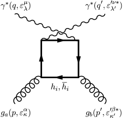
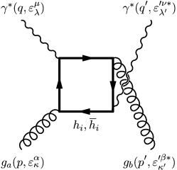
The lowest-order Feynman diagrams that contribute to photon-gluon scattering are shown in Fig. 2.

(a)

(b)

(c)

Figure 2: Lowest order Feynman diagrams for photon-gluon scattering with color indices $a,b,i$. The diagrams that have the heavy quark $h_{i}$ direction reversed are indicated by $\text{$h$\makebox[5.55557pt]{\hskip 0.86108pt$\overline{\phantom{\mathrm{h}}}$}}_{i}$.

The diagrams with the quark direction reversed are not shown separately but are indicated as antiquark loops. Even though the reversion leads to topologically different diagrams in configuration space, their evaluation leads to the same result and is taken into account by an overall factor of two in the following PGS amplitude in $D$ dimensions

$$\mspace{-18.0mu}{\mathop{t_{ba}^{\beta\nu\alpha\mu}}=ie_{h}^{2}g^{2}\operatorname{\delta}_{ba}T_{F}\int\frac{\mathop{\mathrm{d}^{D}{k}}}{(2\pi)^{D}}}$$

$$\times 2\operatorname{Tr}\left[\frac{\gamma^{\alpha}(\text{$k$\makebox[5.52084pt]{/}}+m_{h})\gamma^{\beta}(\text{$k$\makebox[5.52084pt]{/}}+\text{$p$\makebox[5.03125pt]{/}}\vphantom{p}^{\prime}+m_{h})\gamma^{\nu}(\text{$k$\makebox[5.52084pt]{/}}+\text{$p$\makebox[5.03125pt]{/}}\vphantom{p}^{\prime}+\text{$q$\makebox[4.8229pt]{/}}\vphantom{q}^{\prime}+m_{h})\gamma^{\mu}(\text{$k$\makebox[5.52084pt]{/}}+\text{$p$\makebox[5.03125pt]{/}}+m_{h})}{\operatorname{\mathnormal{D}}_{k}(0,m_{h})\operatorname{\mathnormal{D}}_{k}(p^{\prime},m_{h})\operatorname{\mathnormal{D}}_{k}(p^{\prime}+q^{\prime},m_{h})\operatorname{\mathnormal{D}}_{k}(p,m_{h})}\right.$$

$$\phantom{\times\operatorname{Tr}}\left.{}+\frac{\gamma^{\alpha}(\text{$k$\makebox[5.52084pt]{/}}+m_{h})\gamma^{\beta}(\text{$k$\makebox[5.52084pt]{/}}+\text{$p$\makebox[5.03125pt]{/}}\vphantom{p}^{\prime}+m_{h})\gamma^{\mu}(\text{$k$\makebox[5.52084pt]{/}}+\text{$p$\makebox[5.03125pt]{/}}-\text{$q$\makebox[4.8229pt]{/}}\vphantom{q}^{\prime}+m_{h})\gamma^{\nu}(\text{$k$\makebox[5.52084pt]{/}}+\text{$p$\makebox[5.03125pt]{/}}+m_{h})}{\operatorname{\mathnormal{D}}_{k}(0,m_{h})\operatorname{\mathnormal{D}}_{k}(p^{\prime},m_{h})\operatorname{\mathnormal{D}}_{k}(p-q^{\prime},m_{h})\operatorname{\mathnormal{D}}_{k}(p,m_{h})}\right.$$

$$\phantom{\times\operatorname{Tr}}\left.{}+\frac{\gamma^{\alpha}(\text{$k$\makebox[5.52084pt]{/}}+m_{h})\gamma^{\nu}(\text{$k$\makebox[5.52084pt]{/}}+\text{$q$\makebox[4.8229pt]{/}}\vphantom{q}^{\prime}+m_{h})\gamma^{\beta}(\text{$k$\makebox[5.52084pt]{/}}+\text{$p$\makebox[5.03125pt]{/}}\vphantom{p}^{\prime}+\text{$q$\makebox[4.8229pt]{/}}\vphantom{q}^{\prime}+m_{h})\gamma^{\mu}(\text{$k$\makebox[5.52084pt]{/}}+\text{$p$\makebox[5.03125pt]{/}}+m_{h})}{\operatorname{\mathnormal{D}}_{k}(0,m_{h})\operatorname{\mathnormal{D}}_{k}(q^{\prime},m_{h})\operatorname{\mathnormal{D}}_{k}(p^{\prime}+q^{\prime},m_{h})\operatorname{\mathnormal{D}}_{k}(p,m_{h})}\right]$$ (16)

with $\operatorname{\mathnormal{D}}_{k}(p,m_{h}):=(k+p)^{2}-m_{h}^{2}+i\epsilon$. The calculation of this amplitude was carried out with the help of Mathematica [30] that provided an adequate handling of the excessive algebra and the Tracer [31] package that was used to evaluate the trace and to contract Lorentz indices. The individual steps that lead to the analytical results are detailed below.

The integral over the loop momentum can be systematically reduced to scalar integrals

$$\int{}\mathop{\mathrm{d}^{D}{k}}\left[\operatorname{\mathnormal{D}}_{k}(0,m_{0})\operatorname{\mathnormal{D}}_{k}(p_{1},m_{1})\cdots\operatorname{\mathnormal{D}}_{k}(p_{N},m_{N})\right]^{-1}$$ (17)

by a Passarino-Veltman decomposition [32] which is described in a form more suitable for implementation in computer algebra systems in Ref. [33]. The whole PGS amplitude in Eq. (3) is finite whereas the separate scalar integrals can be divergent. Therefore the general $D$ dimensions have to be kept to regularize any divergences during intermediate steps. Explicit formulas for the scalar integrals are given in Refs. [34, 35, 33] in which they are expressed in terms of complex (di)logarithms whose arguments are generically built up by

$$\operatorname{\mathnormal{r}}_{s}:=\frac{\operatorname{\beta}_{s}-1}{\operatorname{\beta}_{s}+1}\quad\text{with}\quad\operatorname{\beta}_{s}:=\sqrt{1-\frac{4m_{h}^{2}}{s+i\epsilon}}$$ (18)

if all masses are equal as it is the case for the lowest order PGS amplitude.

The immediate application of the Passarino-Veltman decomposition to Eq. (3) is in principle possible but not practical. The amount of work is considerably reduced if one gets rid of the four free Lorentz indices first. Inspired by Refs. [36, 37] covariant tensors with an obvious physical meaning are constructed that appear as independent Lorentz structures in the PGS amplitude and equally act as projectors onto them. The three covariant four-vectors

$$\tilde{\varepsilon}_{2}^{\smash{\mu}}:=\frac{\eta^{\prime\mu}-{\eta^{\prime}}{\cdot}{\eta}\eta^{\mu}-{\eta^{\prime}}{\cdot}{\hat{q}}\hat{q}^{\mu}}{\sqrt{({\eta^{\prime}}{\cdot}{\eta})^{2}-({\eta^{\prime}}{\cdot}{\hat{q}})^{2}-\eta^{\prime 2}}}\;,\quad\tilde{\varepsilon}_{1}^{\smash{\mu}}:=-\varepsilon_{\kappa\lambda\phantom{\mu}\nu}^{\phantom{\kappa\lambda}\smash{\mu}}\eta^{\kappa}\hat{q}^{\lambda}\tilde{\varepsilon}_{2}^{\nu}\;,\quad\tilde{\varepsilon}_{0}^{\smash{\mu}}:=\frac{{\eta}{\cdot}{q}q^{\mu}-q^{2}\eta^{\mu}}{\sqrt{-q^{2}}\sqrt{({\eta}{\cdot}{q})^{2}-q^{2}}}$$ (19)

$$\text{with}\quad\hat{q}^{\mu}:=\frac{q^{\mu}-{q}{\cdot}{\eta}\eta^{\mu}}{\sqrt{({q}{\cdot}{\eta})^{2}-q^{2}}}\;,\quad\eta^{2}=1\;,\quad$$

$\eta^{\prime}$ defining the direction of $\tilde{\varepsilon}_{2}$, and definite parity serve as a basis. One easily proves that they reduce to the usual linear polarization vectors of the incoming photon in the frame $\vec{\eta}=\vec{\text{{0}}}$. Now the sought-for tensors are simple products of these polarization vectors and analogous ones for $\alpha,\beta,\mu$ with the sensible choice $\eta\sim\text{$p$\makebox[5.55557pt]{\hskip 0.86108pt$\overline{\phantom{\mathrm{p}}}$}}\vphantom{p}+\text{$q$\makebox[5.27779pt]{\hskip 0.86108pt$\overline{\phantom{\mathrm{q}}}$}}\vphantom{q}=p+q$ and $\eta^{\prime}=\text{$q$\makebox[5.27779pt]{\hskip 0.86108pt$\overline{\phantom{\mathrm{q}}}$}}\vphantom{q}$. Note that the totally antisymmetric epsilon tensor always appears in pairs as the PGS amplitude is parity-even. These products are easily generalized to $D$ dimensions if they are expressed by metric tensors. Physically, this means a sum over polarization vectors that are perpendicular to the scattering plane. In principle this sum has to be normalized by a factor $1/(D-3)$ which is, however, not necessary for the finite PGS amplitude in Eq. (3).

The complex circular polarization vectors used in the expansion of the Compton amplitude in Eq. (6) are given by

$$\varepsilon_{\pm}^{\smash{\mu}}:=\mp\frac{1}{\sqrt{2}}\left(\tilde{\varepsilon}_{1}^{\smash{\mu}}\pm{}i\tilde{\varepsilon}_{2}^{\smash{\mu}}\right)\;,\quad\varepsilon_{0}^{\smash{\mu}}:={}i\tilde{\varepsilon}_{0}^{\smash{\mu}}\;.$$ (20)

From a parton model point of view it looks advantageous to use $\eta\sim\text{$p$\makebox[5.55557pt]{\hskip 0.86108pt$\overline{\phantom{\mathrm{p}}}$}}\vphantom{p}$ because in this case these polarization vectors are invariant under the replacement $\text{$p$\makebox[5.55557pt]{\hskip 0.86108pt$\overline{\phantom{\mathrm{p}}}$}}\vphantom{p}\to{}y\text{$p$\makebox[5.55557pt]{\hskip 0.86108pt$\overline{\phantom{\mathrm{p}}}$}}\vphantom{p}$. Anyway, both choices are equivalent on the leading twist level and lead to the same hard scattering coefficients that are presented in the next section.

In order to extract the leading twist contribution, one has to consider the limit $t\to 0$ where some care has to be taken since factors up to $t^{2}$ that appear in denominators which originate from the normalization of the polarization vectors have to be canceled thoroughly. In this limit the dilogarithms drop out completely.

4 Analytical results

At the leading twist-two level the general Compton amplitude with virtual photons in the initial and final state receives contributions of gluons inside the proton to the following form factors

$$\mathop{T^{\nu\mu}}={} \sum_{\lambda=\pm}\varepsilon^{\prime\nu\vphantom{\mu}}_{\lambda}\varepsilon_{\lambda}^{\mu\ast\vphantom{\mu}}\mathop{T_{\text{T}}}+\sum_{\lambda=\pm}\lambda\varepsilon^{\prime\nu\vphantom{\mu}}_{\lambda}\varepsilon_{\lambda}^{\mu\ast\vphantom{\mu}}\mathop{\widetilde{T}_{\text{T}}}+\varepsilon^{\prime\nu\vphantom{\mu}}_{0}\varepsilon_{0}^{\mu\ast\vphantom{\mu}}\mathop{T_{\text{L}}}$$

$$+\sum_{\lambda=\pm}\varepsilon^{\prime\nu\vphantom{\mu}}_{-\lambda}\varepsilon_{\lambda}^{\mu\ast\vphantom{\mu}}\mathop{T_{\overline{\text{T}}}}+\sum_{\lambda=\pm}\lambda\varepsilon^{\prime\nu\vphantom{\mu}}_{-\lambda}\varepsilon_{\lambda}^{\mu\ast\vphantom{\mu}}\mathop{\widetilde{T}_{\overline{\text{T}}}}+\ldots$$ (21)

where the three additional terms in comparison to Eq. (6) are related to longitudinally polarized photons (L) and to photon helicity flip ($\overline{\text{T}}$). Due to the real photon in the final state $\mathop{T_{\text{L}}}$ does not appear in the DVCS amplitude. From the calculation of PGS that has been sketched in the last section it is possible to obtain the lowest-order massive hard scattering coefficients appearing in factorization theorems for these form factors like in Eq. (9). Now it will be indicated how they are extracted from the amplitude in Eq. (3).

Generally, the squared heavy quark charge already appears in the factorization formula, the QCD coupling constant is extracted in accordance to Eq. (11), and one gets an additional factor $1/[2(1-\xi^{2})]$ from the normalization of the gluon GPDs [16, 25]. The massive hard scattering coefficients relevant for the numerical analysis in the next section are contained in the gluon polarization vector sums $\sum_{\lambda=\pm}\varepsilon^{\prime\beta\vphantom{\mu}}_{\lambda}\varepsilon_{\lambda}^{\alpha\ast\vphantom{\mu}}$ for $\mathop{T_{\text{T}}}$, resp. $\sum_{\lambda=\pm}\lambda\varepsilon^{\prime\beta\vphantom{\mu}}_{\lambda}\varepsilon_{\lambda}^{\alpha\ast\vphantom{\mu}}$ for $\mathop{\widetilde{T}_{\text{T}}}$ and read

$$\mathop{t_{\text{T},hg}^{(1)}} =-\frac{T_{F}}{2(1-\xi^{2})^{2}}\left\{\left[x^{2}-\xi^{2}+(1-x)^{2}+4\text{$\eta$\makebox[4.9653pt]{\hskip 0.86108pt$\overline{\phantom{\mathrm{\eta}}}$}}\vphantom{\eta}{}x(1-x)-8\text{$\eta$\makebox[4.9653pt]{\hskip 0.86108pt$\overline{\phantom{\mathrm{\eta}}}$}}\vphantom{\eta}^{2}x^{2}\right]\log^{2}\operatorname{\mathnormal{r}}_{\hat{s}}\right.$$

$$\phantom{{}=-\frac{T_{F}}{2(1-\xi^{2})^{2}}}\vphantom{\frac{T_{F}}{(1-\xi^{2})^{2}}}\left.{}+2\left[(1-2x)^{2}-\xi^{2}+4\text{$\eta$\makebox[4.9653pt]{\hskip 0.86108pt$\overline{\phantom{\mathrm{\eta}}}$}}\vphantom{\eta}{}x(1-x)\right]\operatorname{\beta}_{\hat{s}}\log\operatorname{\mathnormal{r}}_{\hat{s}}\right.$$

$$\phantom{{}=-\frac{T_{F}}{2(1-\xi^{2})^{2}}}\vphantom{\frac{T_{F}}{(1-\xi^{2})^{2}}}\left.{}-\left[\left(\vphantom{\xi^{2}}x/\xi+1-2\text{$\eta$\makebox[4.9653pt]{\hskip 0.86108pt$\overline{\phantom{\mathrm{\eta}}}$}}\vphantom{\eta}{}x/\xi\right)\left(1+2x\xi-\xi^{2}\right)-4\text{$\eta$\makebox[4.9653pt]{\hskip 0.86108pt$\overline{\phantom{\mathrm{\eta}}}$}}\vphantom{\eta}{}x\xi-8\text{$\eta$\makebox[4.9653pt]{\hskip 0.86108pt$\overline{\phantom{\mathrm{\eta}}}$}}\vphantom{\eta}^{2}x^{2}\right]\log^{2}\operatorname{\mathnormal{r}}_{q^{2}}\right.$$

$$\phantom{{}=-\frac{T_{F}}{2(1-\xi^{2})^{2}}}\vphantom{\frac{T_{F}}{(1-\xi^{2})^{2}}}\left.{}-2\left(\vphantom{\xi^{2}}x/\xi+1\right)\left(1+4x\xi-\xi^{2}-4\text{$\eta$\makebox[4.9653pt]{\hskip 0.86108pt$\overline{\phantom{\mathrm{\eta}}}$}}\vphantom{\eta}{}x\xi\right)\operatorname{\beta}_{q^{2}}\log\operatorname{\mathnormal{r}}_{q^{2}}+(x\to{-x})\right\}$$

$$\mathop{\tilde{t}_{\text{T},hg}^{(1)}} =\frac{T_{F}}{2(1-\xi^{2})^{2}}\left[\left(1-2x+\xi^{2}\right)\log^{2}\operatorname{\mathnormal{r}}_{\hat{s}}+2\left(3-4x+\xi^{2}\right)\operatorname{\beta}_{\hat{s}}\log\operatorname{\mathnormal{r}}_{\hat{s}}\right.$$

$$\phantom{{}=\frac{T_{F}}{2(1-\xi^{2})^{2}}}\vphantom{\frac{T_{F}}{(1-\xi^{2})^{2}}}\left.{}+2\left(\vphantom{\operatorname{\beta}_{q^{2}}}x+\xi\right)\left(\log^{2}\operatorname{\mathnormal{r}}_{q^{2}}+4\operatorname{\beta}_{q^{2}}\log\operatorname{\mathnormal{r}}_{q^{2}}\right)-(x\to{-x})\right]$$ (22)

with $\text{$\eta$\makebox[4.9653pt]{\hskip 0.86108pt$\overline{\phantom{\mathrm{\eta}}}$}}\vphantom{\eta}:={}m_{h}^{2}/\text{$Q$\makebox[7.7778pt]{\hskip 0.86108pt$\overline{\phantom{\mathrm{Q}}}$}}\vphantom{Q}^{2}$. The corresponding results for massless quarks [25, 28] are obtained for $\text{$\eta$\makebox[4.9653pt]{\hskip 0.86108pt$\overline{\phantom{\mathrm{\eta}}}$}}\vphantom{\eta}\to 0$ with appropriate subtraction of the logarithmic divergences $\sim\log(m_{h}/\mu)$. It should be remarked that the limits have to be taken in this order, namely, first $t\to 0$ and then $\text{$\eta$\makebox[4.9653pt]{\hskip 0.86108pt$\overline{\phantom{\mathrm{\eta}}}$}}\vphantom{\eta}\to 0$, to reproduce the massless results.

Furthermore, the contraction of the gluonic Lorentz indices analogously to $\mathop{T_{\text{T}}}$ gives the contribution of longitudinally polarized photons

$$\mathop{t_{\text{L},hg}^{(1)}}=\frac{2T_{F}\sqrt{\lvert{1-\xi^{2}/x^{2}}\rvert}}{(1-\xi^{2})^{2}} \left[2\text{$\eta$\makebox[4.9653pt]{\hskip 0.86108pt$\overline{\phantom{\mathrm{\eta}}}$}}\vphantom{\eta}{}x^{2}\left(\log^{2}\operatorname{\mathnormal{r}}_{\hat{s}}-\log^{2}\operatorname{\mathnormal{r}}_{q^{2}}\right)+2x(1-x)\operatorname{\beta}_{\hat{s}}\log\operatorname{\mathnormal{r}}_{\hat{s}}\right.$$

$$\vphantom{\frac{T_{F}}{(1-\xi^{2})^{2}}}\left.{}+\left(x/\xi+2x^{2}+x\xi\right)\operatorname{\beta}_{q^{2}}\log\operatorname{\mathnormal{r}}_{q^{2}}+(x\to{-x})\right]\;.$$ (23)

The “massless” limit can be achieved in the same way as mentioned above but will not be explicitly stated since it is not needed at present.

As a byproduct of the calculation of the PGS amplitude with the method presented in the previous section one also gets massive expressions for the hard scattering coefficients in factorization theorems with generalized helicity-flip, or tensor gluon distributions, respectively, whose exact definitions and applications are given in Refs. [38, 39, 40]. They have to be projected from the gluon polarization vector sums $\sum_{\lambda=\pm}\varepsilon^{\prime\beta\vphantom{\mu}}_{-\lambda}\varepsilon_{\lambda}^{\alpha\ast\vphantom{\mu}}$ for $\mathop{T_{\overline{\text{T}}}}$ and $\sum_{\lambda=\pm}\lambda\varepsilon^{\prime\beta\vphantom{\mu}}_{-\lambda}\varepsilon_{\lambda}^{\alpha\ast\vphantom{\mu}}$ for $\mathop{\widetilde{T}_{\overline{\text{T}}}}$ and are given for completeness

$$\mathop{t_{\overline{\text{T}},hg}^{(1)}}=\mathop{\tilde{t}_{\overline{\text{T}},hg}^{(1)}}=\frac{2T_{F}}{(1-\xi^{2})^{2}} \left[2\text{$\eta$\makebox[4.9653pt]{\hskip 0.86108pt$\overline{\phantom{\mathrm{\eta}}}$}}\vphantom{\eta}(1+\text{$\eta$\makebox[4.9653pt]{\hskip 0.86108pt$\overline{\phantom{\mathrm{\eta}}}$}}\vphantom{\eta})x^{2}\left(\log^{2}\operatorname{\mathnormal{r}}_{\hat{s}}-\log^{2}\operatorname{\mathnormal{r}}_{q^{2}}\right)-2\text{$\eta$\makebox[4.9653pt]{\hskip 0.86108pt$\overline{\phantom{\mathrm{\eta}}}$}}\vphantom{\eta}{}x(1+\xi)\operatorname{\beta}_{\hat{s}}\log\operatorname{\mathnormal{r}}_{\hat{s}}\right.$$

$$\vphantom{\frac{T_{F}}{(1-\xi^{2})^{2}}}\left.{}-\left(\vphantom{\operatorname{\beta}_{q^{2}}}x+\xi\right)\left(\vphantom{\operatorname{\beta}_{q^{2}}}x-\xi-2\text{$\eta$\makebox[4.9653pt]{\hskip 0.86108pt$\overline{\phantom{\mathrm{\eta}}}$}}\vphantom{\eta}{}x\right)\left(\operatorname{\beta}_{\hat{s}}\log\operatorname{\mathnormal{r}}_{\hat{s}}-\operatorname{\beta}_{q^{2}}\log\operatorname{\mathnormal{r}}_{q^{2}}\right)+(x\to{-x})\right]$$

$${}+\frac{2T_{F}}{1-\xi^{2}} \;.$$ (24)

The limit $\text{$\eta$\makebox[4.9653pt]{\hskip 0.86108pt$\overline{\phantom{\mathrm{\eta}}}$}}\vphantom{\eta}\to 0$ is finite as expected because the generalized tensor gluon distributions do not mix with any quark distributions and reproduces the “massless” results of Refs. [38, 39].

Two further limits provide additional checks for the mass dependencies in Eq. (4). On the one hand the contributions of heavy quarks do vanish for infinitely large masses in accordance with the decoupling theorem [41]. On the other hand the imaginary parts of Eqs. (4) and (4) in the forward scattering limit are given by

$$\frac{1}{\pi}\operatorname{Im}{}\mathop{t_{\text{T},hg}^{(1)}}\xrightarrow{\xi\to{}0}-T_{F}\operatorname{\theta}(1/x-1-4\eta)$$

$$\qquad\vphantom{\frac{1}{\pi}}\times\left\{\left[x^{2}+(1-x)^{2}+4\eta{}x(1-x)-8\eta^{2}x^{2}\right]\log(-\operatorname{\mathnormal{r}}_{\hat{s}})+\left[(1-2x)^{2}+4\eta{}x(1-x)\right]\operatorname{\beta}_{\hat{s}}\right\}$$

$$\frac{1}{\pi}\operatorname{Im}{}\mathop{t_{\text{L},hg}^{(1)}}\xrightarrow{\xi\to{}0}4T_{F}\operatorname{\theta}(1/x-1-4\eta)\left[2\eta{}x^{2}\log(-\operatorname{\mathnormal{r}}_{\hat{s}})+x(1-x)\operatorname{\beta}_{\hat{s}}\right]$$

$$\frac{1}{\pi}\operatorname{Im}{}\mathop{\tilde{t}_{\text{T},hg}^{(1)}}\xrightarrow{\xi\to{}0}T_{F}\operatorname{\theta}(1/x-1-4\eta)\left[(1-2x)\log(-\operatorname{\mathnormal{r}}_{\hat{s}})+(3-4x)\operatorname{\beta}_{\hat{s}}\right]$$ (25)

with $\eta:={}m_{h}^{2}/Q^{2}$. They coincide with the corresponding quantities of the DIS structure functions $(F_{2}-F_{L})/x$, $F_{L}/x$ [42], and $2g_{1}$ [43] in view of the factorization theorem Eq. (9) as demanded by the optical theorem.

Finally the relevant results for the numerical analysis in the following section are the massive DVCS coefficient functions as defined by Eq. (2)

$$\mathop{C_{\text{T},hg}^{(1)}}(z,Q^{2},\mu)=\frac{T_{F}}{2(z+1)^{2}} \left\{\frac{2-z(6-16\eta)}{z-1}\left(\operatorname{\beta}_{\hat{s}}\log\operatorname{\mathnormal{r}}_{\hat{s}}-\operatorname{\beta}_{q^{2}}\log\operatorname{\mathnormal{r}}_{q^{2}}\right)\right.$$

$$\vphantom{\frac{T_{F}}{(1-\xi^{2})^{2}}}\left.{}-\left[1+8\eta{}z\frac{1-(1+4\eta)z}{(z-1)^{2}}\right]\log^{2}\operatorname{\mathnormal{r}}_{\hat{s}}\right.$$

$$\vphantom{\frac{T_{F}}{(1-\xi^{2})^{2}}}\left.{}+\left[1-2\eta\frac{1+(3+8\eta)z^{2}}{(z-1)^{2}}\right]\log^{2}\operatorname{\mathnormal{r}}_{q^{2}}\right\}$$

$$\mathop{\widetilde{C}_{\text{T},hg}^{(1)}}(z,Q^{2},\mu)=\frac{T_{F}}{2(z+1)^{2}} \left[\frac{2z-6}{z-1}\left(\operatorname{\beta}_{\hat{s}}\log\operatorname{\mathnormal{r}}_{\hat{s}}-\operatorname{\beta}_{q^{2}}\log\operatorname{\mathnormal{r}}_{q^{2}}\right)+\log^{2}\operatorname{\mathnormal{r}}_{\hat{s}}-\log^{2}\operatorname{\mathnormal{r}}_{q^{2}}\right]$$ (26)

that are achieved by enforcing the DVCS kinematics $x\to\xi$. In the combinations of Eq. (2) they are finite for $z\to 1$ and the imaginary parts stem exclusively from the complex logarithms. The arbitrariness in the representations of DVCS coefficient functions is exploited so that Eq. (4) reduces to its equivalent in Eq. (2) for $\eta\to 0$ apart from the logarithmic divergences $\sim\log(m_{h}/\mu)$.

5 Numerical results

A suitable model for the GPDs to employ in a first numerical analysis of heavy quark effects is given by the moment-diagonal model defined in Ref. [44]. One can expect that it leads to the same difficulties to describe experimental data, which is explained in detail in Ref. [45], as factorized double distribution based models for GPDs [46]. Nevertheless moment diagonal models have important advantages. They are scale independently related to the conventional forward parton distribution functions (PDFs) so that no additional GPD input scale uncertainty is introduced and their dependence on the specific forward PDF set is reduced. Therefore, the following results should be unique consequences of heavy quark contributions. Apart from that, the evaluation of the form factors of the DVCS amplitude can be performed in a numerically very stable way without any principal value integrals [44]. The utilized unpolarized and polarized forward PDFs are GRV(98) [21] and the standard scenario of GRSV(00) [47], respectively, with three fixed light flavors. The charm and bottom quark masses are $m_{c}=1.4\,\text{GeV}$ and $m_{b}=4.5\,\text{GeV}$. In accordance to (15) and Ref. [24], intrinsic “massless” (off-)forward heavy quark distribution functions were generated from the same inputs. It should be noted that all the following fixed-order (FO) and “massless” parton (MP) results for the three light quarks $u,d,s$ agree within $1.5\%$.

In Fig. 3

Figure 3: The imaginary and real part of the form factor $\mathop{T_{\text{T},1}}$, related to $\mathop{H}$ in the appropriately substituted Eq. (9), of the DVCS amplitude as a function of $Q^{2}$ at fixed $\xi=10^{-3}$ and $t=0$ for three light flavors (solid line), with the fixed order charm contribution (dashed line), with the “massless” charm (dashed-dotted line) and additionally bottom (dotted line) contribution.

the results for the form factor $\mathop{T_{\text{T},1}}(\xi,t,Q^{2})$ of the DVCS amplitude, which is the one that depends on $\mathop{H}(x,\xi,t,\mu)$, are presented as a function of $Q^{2}$ for vanishing $t$ and fixed $\xi=10^{-3}$ which is representative for the kinematic region of DVCS measurements by H1 [6] and by ZEUS [7] at DESY-HERA. The contributions of the intrinsic “massless” heavy quark GPDs show as expected a different threshold behavior compared to the fixed order results. The former start rather abrupt at $Q^{2}=m_{h}^{2}$ in the imaginary and real part whereas the latter set in smoothly at $\hat{s}>4m_{h}^{2}$ in the imaginary part and contributes to the real part at any scale, though not sizeably for $Q^{2}\ll m_{h}^{2}$. Between the threshold region and the highest $Q^{2}=100\,\text{GeV}^{2}$ displayed in Fig. 3 with the “massless” charm quark contribution in MP udsc lies significantly above the fixed order result FO udsc. The small “massless” bottom quark contribution justifies to neglect all further bottom results from now on, as it has been already done for the nearly vanishing fixed order bottom results in Fig. 3.

The corresponding results with fixed $\xi=10^{-1}$ relevant for the kinematic region of HERMES [4] and CLAS [5] are shown in Fig. 4.

Figure 4: The imaginary and real parts of the form factors $\mathop{T_{\text{T},1}}$ and $\mathop{\widetilde{T}_{\text{T},\text{A}}}$, related to $\mathop{H}$ and $\mathop{\widetilde{H}}$, respectively, of the DVCS amplitude as a function of $Q^{2}$ at fixed $\xi=10^{-1}$ and $t=0$ for three light flavors (solid line), with the fixed order charm contribution (dashed line), and with the “massless” charm (dashed-dotted line) contribution.

In this case the helicity dependent form factor $\mathop{\widetilde{T}_{\text{T},\text{A}}}(\xi,t,Q^{2})$, which is the one that depends on $\mathop{\widetilde{H}}(x,\xi,t,\mu)$ in the appropriately substituted Eq. (9), is also presented. At even smaller values of $\xi$, e. g. $\xi=10^{-3}$ in Fig. 3, $\mathop{\widetilde{T}_{\text{T},\text{A}}}$ becomes entirely negligible compared to $\mathop{T_{\text{T},1}}$. The “massless” parton prescription still leads to considerable charm contributions whereas the fixed order charm results are marginal. Generally the corrections to DVCS observables due to heavy quarks get larger for increasing $Q^{2}$ and in particular for decreasing $\xi$. Therefore phenomenologically relevant effects have to be expected mainly for the DVCS cross section measurements at H1 and ZEUS.

The DVCS cross section was defined by using the equivalent photon approximation in Ref. [6]. An approximate formula is given by [10]

$$\sigma_{\text{DVCS}}\approx\frac{\pi\alpha^{2}x_{B}^{2}}{Q^{4}b}\left\lvert{\mathop{T_{\text{T},1}}(\xi,0,Q^{2})}\right\rvert^{2}$$ (27)

where $b$ is a measure of the $t$-dependence of the DVCS amplitude and currently expected to be nearly constant. In Fig. 5

Figure 5: The DVCS cross section as a function of $Q^{2}$ at fixed $W=89\,\text{GeV}$ for three light flavors (solid line), with the fixed order charm contribution (dashed line), and with the “massless” charm (dashed-dotted line), using a constant $b[\text{GeV}^{-2}]=4.9$ as well as a strongly $Q^{2}$-dependent $b(Q^{2})[\text{GeV}^{-2}]=4.9-5\log(Q^{2}[\text{GeV}]/100)$. The error bars denote the quadratic sums of the statistical and the systematic uncertainties of the ZEUS data [7].

the results for the DVCS cross section together with the ZEUS data at fixed $W=\sqrt{\hat{s}}=89\,\text{GeV}$ [7] are shown for a constant $b[\text{GeV}^{-2}]=4.9$ as it has been used by the ZEUS collaboration and additionally for a highly $Q^{2}$ dependent $b(Q^{2})[\text{GeV}^{-2}]=4.9-5\log(Q^{2}[\text{GeV}]/100)$. The constant $b$ shows the aforementioned difficulties by overshooting the data considerably that is basically in line with previous leading order predictions [10]. Only recently it was found that a “$k$-delta ansatz” [48] with $k=0$, i. e. a narrow $y$-dependence for the double distribution $F(x,y)$, can be used to describe the data [13]. However, such an ansatz is considered not realistic since it does not fulfill a certain symmetry constraint for double distributions [49, 48].

The simple highly $Q^{2}$ dependent $b$-fit that yields a good agreement of the light flavor result with the data should merely give an impression of the relevance of charm contributions. The fixed order charm contributions increase the DVCS cross section by $10\%$ for the lowest $Q^{2}$ shown and up to $30\%$ for large $Q^{2}$ which is beyond the relative uncertainties of the first four data points. The “massless” charm GPD leads to significantly larger increases in the range of $60\ldots 90\%$ which excessively overestimates the physical PGS subprocess. To check for the reliability of this result the CTEQ4 forward PDFs [50] have been used alternatively that give minor modifications less than $10\%$ apart from a reduction of up to $15\%$ around $Q^{2}\sim 10\,\text{GeV}^{2}$ that can be traced back to the higher charm mass $m_{c}^{\text{CTEQ}}=1.6\,\text{GeV}$ and the correspondingly delayed generation of charm. Finally it should be noted that a change of the factorization scale $\mu_{h}\to\sqrt{4m_{h}^{2}+Q^{2}}$ changes the fixed order results below the percent level.

6 Conclusions and outlook

The contributions of heavy quarks, especially of the charm quark, to deeply virtual Compton scattering have been adequately analyzed by fixed order perturbation theory via photon-gluon scattering. The use of intrinsic “massless” generalized heavy quark distributions overestimates the DVCS cross section at small skewedness $\lesssim{}10^{-3}$. In principle this may be absorbed in models for GPDs, which, however, is unreasonable since the fixed order calculation correctly describes at least the threshold region. At large scales $Q^{2}$ both treatments cannot be distinguished because of present experimental uncertainties.

The rough estimates indicate that heavy quark mass effects are relevant for small skewedness $\lesssim 10^{-3}$ in particular at low scales with respect to experimental uncertainties. Nevertheless this should be confirmed with “realistic” GPD models and using the full DVCS amplitude, possibly with higher twist corrections. For values of the skewedness $\sim{}0.1$, characteristic for fixed-target experiments, contributions of heavy quarks can safely be neglected. The massive analytical results for the photon helicity flip form factors of the DVCS amplitude have not been utilized but can be trivially included in future analyses. In this case, the massive description for heavy quarks should always be used as it smoothly reproduces a “massless” parton picture at high scales.

To prove the perturbative stability of the PGS model the next-to-lowest order corrections to the massive hard scattering coefficients have to be calculated which are necessary for a consistent next-to-leading order analysis with heavy quarks correctly included.

References

• [1] X. Ji, Phys. Rev. Lett. 78, 610 (1997).
• [2] A. V. Radyushkin, Phys. Lett. B 380, 417 (1996).
• [3] X. Ji, Phys. Rev. D 55, 7114 (1997).
• [4] A. Airapetian et al. (HERMES), Phys. Rev. Lett. 87, 182001 (2001).
• [5] S. Stepanyan et al. (CLAS), Phys. Rev. Lett. 87, 182002 (2001).
• [6] C. Adloff et al. (H1), Phys. Lett. B 517, 47 (2001).
• [7] S. Chekanov et al. (ZEUS), Phys. Lett. B 573, 46 (2003).
• [8] A. V. Belitsky, D. Müller, L. Niedermeier, and A. Schäfer, Nucl. Phys. B 593, 289 (2001).
• [9] A. Freund and M. F. McDermott, Phys. Rev. D 65, 091901(R) (2002).
• [10] A. Freund and M. F. McDermott, Eur. Phys. J. C 23, 651 (2002).
• [11] N. Kivel, M. V. Polyakov, and M. Vanderhaeghen, Phys. Rev. D 63, 114014 (2001).
• [12] A. V. Belitsky, D. Müller, and A. Kirchner, Nucl. Phys. B 629, 323 (2002).
• [13] A. Freund, Phys. Rev. D 68, 096006 (2003).
• [14] D. Müller, D. Robaschik, B. Geyer, F.-M. Dittes, and J. Hořejši, Fortschr. Phys. 42, 101 (1994).
• [15] A. V. Radyushkin, Phys. Lett. B 385, 333 (1996).
• [16] J. C. Collins, L. L. Frankfurt, and M. Strikman, Phys. Rev. D 56, 2982 (1997).
• [17] M. Burkardt, Phys. Rev. D 62, 071503(R) (2000); 66, 119903(E) (2002).
• [18] M. Diehl, Phys. Rep. 388, 41 (2003).
• [19] C. Adloff et al. (H1), Phys. Lett. B 528, 199 (2002).
• [20] S. Chekanov et al. (ZEUS), Measurement of $D^{\ast\pm}$ production in deep inelastic $e^{\pm}p$ scattering at HERA, hep-ex/0308068.
• [21] M. Glück, E. Reya, and A. Vogt, Eur. Phys. J. C 5, 461 (1998).
• [22] B. W. Harris and J. Smith, Nucl. Phys. B 452, 109 (1995); Phys. Rev. D 57, 2806 (1998).
• [23] M. Glück, E. Reya, and M. Stratmann, Nucl. Phys. B 422, 37 (1994).
• [24] J. C. Collins and W.-K. Tung, Nucl. Phys. B 278, 934 (1986).
• [25] X. Ji and J. Osborne, Phys. Rev. D 58, 094018 (1998).
• [26] A. V. Radyushkin, Phys. Rev. D 56, 5524 (1997).
• [27] J. C. Collins and A. Freund, Phys. Rev. D 59, 074009 (1999).
• [28] A. V. Belitsky, D. Müller, L. Niedermeier, and A. Schäfer, Phys. Lett. B 474, 163 (2000).
• [29] A. V. Belitsky, A. Freund, and D. Müller, Nucl. Phys. B 574, 347 (2000).
• [30] Wolfram Research, Inc., Mathematica (Wolfram Research, Inc., Champaign, Illinois, 2001), Version 4.1.
• [31] M. Jamin and M. E. Lautenbacher, Comp. Phys. Comm. 74, 265 (1993).
• [32] G. Passarino and M. Veltman, Nucl. Phys. B 160, 151 (1979).
• [33] A. Denner, Fortschr. Phys. 41, 307 (1993).
• [34] G. ’t Hooft and M. Veltman, Nucl. Phys. B 153, 365 (1979).
• [35] A. Denner, U. Nierste, and R. Scharf, Nucl. Phys. B 367, 637 (1991).
• [36] V. M. Budnev, I. F. Ginzburg, G. V. Meledin, and V. G. Serbo, Phys. Rep. 15, 181 (1975).
• [37] I. Schienbein, Ann. Phys. (NY) 301, 128 (2002).
• [38] P. Hoodbhoy and X. Ji, Phys. Rev. D 58, 054006 (1998).
• [39] A. V. Belitsky and D. Müller, Phys. Lett. B 486, 369 (2000).
• [40] M. Diehl, Eur. Phys. J. C 19, 485 (2001).
• [41] T. Appelquist and J. Carazzone, Phys. Rev. D 11, 2856 (1975).
• [42] E. Witten, Nucl. Phys. B 104, 445 (1976).
• [43] M. Glück, E. Reya, and W. Vogelsang, Nucl. Phys. B 351, 579 (1991).
• [44] J. D. Noritzsch, Phys. Rev. D 62, 054015 (2000).
• [45] A. Freund, M. F. McDermott, and M. Strikman, Phys. Rev. D 67, 036001 (2003).
• [46] A. V. Radyushkin, Phys. Lett. B 449, 81 (1999).
• [47] M. Glück, E. Reya, M. Stratmann, and W. Vogelsang, Phys. Rev. D 63, 094005 (2001).
• [48] A. V. Radyushkin, Phys. Rev. D 59, 014030 (1998).
• [49] L. Mankiewicz, G. Piller, and T. Weigl, Eur. Phys. J. C 5, 119 (1998).
• [50] H. L. Lai et al., Phys. Rev. D 55, 1280 (1997).