MPP-2003-134

FTUAM-03-23

IFT-UAM/CSIC-03-52

SUSY-electroweak one-loop contributions to
Flavour-Changing Higgs-Boson Decays

A. M. Curiel${}^{\,\scriptstyle{a}}$, M. J. Herrero${}^{\,\scriptstyle{a}}$, W. Hollik${}^{\,\scriptstyle{b}}$, F. Merz${}^{\,\scriptstyle{b}}$ and S. Peñaranda${}^{\,\scriptstyle{b}}$  
a: Departamento de Física Teórica, Universidad Autónoma de Madrid, Cantoblanco, 28049 Madrid, Spain.
b: Max-Planck-Institut für Physik, Föhringer Ring 6, D–80805 Munich, Germany

Abstract

The SUSY-EW one-loop quantum contributions to flavour-changing MSSM Higgs-boson decays into $b\bar{s}$ and $s\bar{b}$ are computed and discussed. We use the full diagrammatic approach that is valid for all $\tan\beta$ values and do not rely on the mass-insertion approximation for the characteristic flavour-changing parameter. We analyze in full detail the dependence of these flavour-changing partial widths on all the relevant MSSM parameters and also study the non-decoupling behaviour of these widths with the SUSY mass parameters. We find that these contributions are sizable as compared to the SM ones, and together with the SUSY-QCD contributions they can be very efficient as an indirect method in the future search for Supersymmetry.

1 Introduction

Rare processes involving Flavour Changing Neutral Currents (FCNC) provide an extremely useful tool to investigate new physics beyond the Standard Model (SM). The strong suppression of FCNC in the SM is due to the absence of tree-level contributions and the smallness of the loop-contributions. The later, being a consequence of the GIM-cancellation mechanism [1], naturally enhances the sensitivity of Flavour Changing (FC) processes to possible non-standard phenomena. Among the various possibilities, the Higgs-mediated FCNC processes involving down-type quarks are particularly interesting since, within the SM, they are additionally suppressed by the smallness of the down-type Yukawa couplings.

The Minimal Supersymmetric Standard Model (MSSM) [2] provides a natural framework where such scalar FC interactions could be significant if the soft SUSY-breaking mass terms contain some non-diagonal structure in flavour space. In the minimal-flavour-violation scenario of the MSSM, squarks are assumed to be aligned with the corresponding quarks. Flavour violation in this case originates from the Cabibbo-Kobayashi-Maskawa (CKM) matrix as the only source, and proceeds via loop-contributions, in analogy to the SM. Therefore, its size is expected to be very small. However, in the more general scenarios that include misalignment between the quark and squark sectors, sizeable contributions to FCNC processes are expected to occur. It is indeed the case of the radiative corrections from SUSY-loops in the context of $B$-meson physics that come with factors of $\tan\beta$, the ratio of the vacuum expectation values of the two MSSM Higgs doublets. These $\tan\beta$-enhanced SUSY radiative corrections have been studied in a number of processes, including $B^{0}-\bar{B}^{0}$ mixing [3, 4], leptonic $B$ meson decays [5, 6, 7, 8], and $b\rightarrow s\gamma$ decays [9, 10, 11, 12], and have been found to be large. In order not to be in conflict with present experimental data, these in turn imply some restrictions on the parameters measuring the size of flavor mixing in the squark sector which, as we have said, is mainly produced from quark–squark misalignment [8, 13, 14, 15].

Other FCNC processes of interest are related to Higgs physics and are also very sensitive to supersymmetric quantum effects [16, 17, 18, 19]. In particular, the neutral MSSM Higgs-boson decays into $b\bar{s}$ and $s\bar{b}$ have been proven to be generated quite efficiently from squark–gluino loops if quark–squark misalignment is assumed [16]. These SUSY-QCD loop contributions have the peculiarity of being non-vanishing even in the limit of very heavy SUSY particles and, in addition, they are enhanced by large $\tan\beta$ factors. Such a non-decoupling behaviour of SUSY particles in the Flavor Changing Higgs Decays (FCHD) can be of special interest for indirect SUSY searches at future colliders, as the forthcoming LHC and a next $e^{+}e^{-}$ linear collider, in particular if the SUSY particles turn out to be too heavy to be produced directly. The large rates found for the SUSY-QCD contributions to the Higgs partial decay widths into $b\bar{s}$ and $s\bar{b}$ [16], as well as to the effective FC Higgs couplings to quarks [5, 6, 7, 8, 17, 18], are indeed quite encouraging.

In this paper we complete the genuine SUSY quantum effects in FCHD by the computation of the SUSY electroweak (SUSY-EW) one-loop contributions to Higgs-boson decays into $b\bar{s}$ and $s\bar{b}$. The dominant SUSY-EW radiative corrections to the effective Higgs-boson couplings to quarks have been computed recently in the mass-insertion approximation, including both misalignment and CKM induce effects [18]. Here we will perform an exact computation of the complete SUSY-EW one-loop contributions from squark–chargino and squark–neutralino loops to the flavour-nondiagonal decay rates of the three neutral MSSM Higgs bosons and compare them with the SUSY-QCD contributions. Since no approximation is used, our computation is valid for all values of the characteristic parameter measuring the squark-mixing strength and for all $\tan\beta$ values. Furthermore, we will explore in detail the dependence of these SUSY-EW quantum contributions on the MSSM parameters, and we will study their behaviour in the large sparticle-mass limit. Both the numerical results and the asymptotic analytical formulas, showing the non-decoupling behaviour, can be of particular interest for future Higgs-physics studies at next-generation colliders.

The paper is organized as follows. Section 2 describes the basis for FC interactions in the SUSY-EW sector of the MSSM. The computation of the SUSY-EW one-loop contributions to the Higgs-$b$-$s$ form factors and Higgs decay widths into $b\bar{s}$ and $s\bar{b}$ are outlined in section 3. The numerical analysis of the FCHD rates and a detailed discussion of the dependence on the relevant MSSM parameters are included in section 4, and the large sparticle-mass limit is studied in section 5. A set of useful and compact formulas valid in this limit is also derived; it is listed in the Appendix, together with other details of the computation.

2 Flavour-changing interactions in the MSSM

In the MSSM there are two sources of FC phenomena. The first one is common to the Standard Model case and is due to mixing in the quark sector. It is produced by the different rotation in the $d$- and $u$-quark sectors, and its strength is driven by the off-diagonal CKM-matrix elements. This mixing produces FC electroweak interaction terms involving charged currents and, in particular, supersymmetric electroweak interaction terms of the chargino–quark–squark type, which are of interest to this work. The second source of FC phenomena is due to the possible misalignment between the rotations that diagonalize the quark and squark sectors. When the squark-mass matrix is expressed in the basis where the squark fields are parallel to the quarks (the super-CKM basis), it is in general non-diagonal in flavour space. This quark–squark misalignment produces new FC terms in neutral-current as well as in charged-current interactions. In the case of the SUSY-QCD sector, the FC interaction terms involve neutral currents of the gluino–quark–squark type, and their effects on FCHD have been studied in ref. [16]. Here we focus on the SUSY-EW interaction terms generating FC phenomena, in particular on those of the neutralino–quark–squark and chargino–quark–squark type. The first one appears exclusively due to quark–squark misalignment, as in the SUSY-QCD case, whereas the second one receives contributions from both sources, quark–squark misalignment and CKM mixing.

We assume here that the non-CKM squark mixing is significant only for transitions between the third- and second-generation squarks, and that there is only LL mixing, given by a similar ansatz as in [20] where it is proportional to the product of the SUSY masses involved. This assumption is theoretically well motivated by the radiatively induced flavour off-diagonal squark squared-mass entries via RGE from high energies down to the electroweak scale [21]. These RGE predict that the flavour changing LL entries scale with the square of the soft-SUSY breaking masses, in contrast with the LR (or RL) and the RR entries that scale with one or zero powers, respectively. Thus, the hierarchy $LL>>LR\,,RL>>RR$ is usually assumed. These same estimates also indicate that the LL entry for the mixing between the second and third generation squarks is the dominant one due to the larger quark mass factors involved. On the other hand, the LR and RL entries are experimentally more constrained, mainly by $b\to s\gamma$ data [14]. With the previous assumption, the squark squared-mass matrices in the ($\tilde{c}_{L}$,$\tilde{c}_{R}$,$\tilde{t}_{L}$,$\tilde{t}_{R}$) and ($\tilde{s}_{L}$,$\tilde{s}_{R}$,$\tilde{b}_{L}$,$\tilde{b}_{R}$) basis, respectively, can be written as follows,

$$M^{2}_{\tilde{u}}=\left\lgroup\begin{array}[]{llll}M_{L,c}^{2}&m_{c}X_{c}&\lambda_{LL}M_{L,c}M_{L,t}&0\\ m_{c}X_{c}&M_{R,c}^{2}&0&0\\ \lambda_{LL}M_{L,c}M_{L,t}&0&M_{L,t}^{2}&m_{t}X_{t}\\ 0&0&m_{t}X_{t}&M_{R,t}^{2}\end{array}\right\rgroup,$$ (2.5)

$$M^{2}_{\tilde{d}}=\left\lgroup\begin{array}[]{llll}M_{L,s}^{2}&m_{s}X_{s}&\lambda_{LL}M_{L,s}M_{L,b}&0\\ m_{s}X_{s}&M_{R,s}^{2}&0&0\\ \lambda_{LL}M_{L,s}M_{L,b}&0&M_{L,b}^{2}&m_{b}X_{b}\\ 0&0&m_{b}X_{b}&M_{R,b}^{2}\end{array}\right\rgroup$$ (2.10)

where

$$M_{L,q}^{2} = M_{\tilde{Q},q}^{2}+m_{q}^{2}+\cos 2\beta(T_{3}^{q}-Q_{q}s_{W}^{2})m_{Z}^{2}\,,$$

$$M_{R,(c,t)}^{2} = M_{\tilde{U},(c,t)}^{2}+m_{c,t}^{2}+\cos 2\beta Q_{t}s_{W}^{2}m_{Z}^{2}\,,$$

$$M_{R,(s,b)}^{2} = M_{\tilde{D},(s,b)}^{2}+m_{s,b}^{2}+\cos 2\beta Q_{b}s_{W}^{2}m_{Z}^{2}\,,$$

$$X_{c,t} = A_{c,t}-\mu\cot\beta\,,$$

$$X_{s,b} = A_{s,b}-\mu\tan\beta\,;$$ (2.11)

$m_{q}$, $T_{3}^{q}$, $Q_{q}$ are the mass, isospin and electric charge of the quark $q$; $m_{Z}$ is the $Z$ boson mass, and $s_{W}=\sin\theta_{W}$ contains the electroweak mixing angle $\theta_{W}$. The relevant MSSM parameters in the SUSY-EW sector are, as usual, the soft SUSY-breaking EW gaugino masses, $M_{1}$ and $M_{2}$, the $\mu$-parameter, the soft SUSY–breaking scalar masses $M_{\tilde{Q}}$, $M_{\tilde{U}}$, $M_{\tilde{D}}$, and the soft SUSY–breaking trilinear parameters, $A_{q}$. Owing to the $SU(2)_{L}$ invariance, $M_{\tilde{Q},c}=M_{\tilde{Q},s}$ and $M_{\tilde{Q},t}=M_{\tilde{Q},b}$. For simplicity, we have assumed the soft-breaking trilinear matrices to be diagonal in flavour space.

In our parametrization (2.5), (2.10) of flavour mixing in the squark sector, there is only one free parameter, $\lambda_{LL}$, that characterizes the flavour-mixing strength. For the sake of simplicity, we assume the same $\lambda_{LL}$ parameter in the $\tilde{t}-\tilde{c}$ and $\tilde{b}-\tilde{s}$ sectors, writing $\lambda\equiv\lambda_{LL}$ from now on for a simpler notation. Obviously, the choice $\lambda=0$ represents the case of zero flavour mixing.

In order to diagonalize the two $4\times 4$ squark-mass matrices given above, two $4\times 4$ matrices, $R^{(u)}$ for the $up$-type squarks and $R^{(d)}$ for the $down$-type squarks, are needed. Diagonalization yields the squark-mass eigenvalues and eigenstates depending on $\lambda$. This dependence has been studied in [16]; typically, two of the eigenvalues are weakly dependent on $\lambda$, with mass values very close to the case with $\lambda=0$, and for the other two, one grows with $\lambda$ and the other decreases with it. For $\lambda=0$, one recovers the usual pairs of physical flavour-diagonal squarks, ($\tilde{b}_{1},\tilde{b}_{2}$), ($\tilde{s}_{1},\tilde{s}_{2}$), ($\tilde{t}_{1},\tilde{t}_{2}$), and ($\tilde{c}_{1},\tilde{c}_{2}$).

The following paragraph presents the SUSY-EW interaction terms that are responsible for flavour-changing neutral Higgs-boson decays. We will write them in the mass-eigenstate basis.

The chargino–quark–squark interactions are described by the interaction Lagrangian

$$\mathcal{L}_{\tilde{\chi}_{j}^{-}d\tilde{u}_{\alpha}} = -g\,\bar{d}\left[A_{L\alpha j}^{(d)}P_{L}+A_{R\alpha j}^{(d)}P_{R}\right]\tilde{\chi}_{j}^{-}\tilde{u}_{\alpha}+h.c.,$$ (2.12)

where $d$ can be either a $b$ or $s$ quark; the chargino index is $j=1,2$ for the two physical states, and the squark index is $\alpha=1,2,3,4$, representing the four physical squark states. $g$ denotes the $SU(2)_{L}$ gauge coupling, and the coefficients $A_{L\alpha j}^{(d)}$ and $A_{R\alpha j}^{(d)}$ are listed in Appendix A. They include the two above commented sources of flavour-changing vertices, quark–squark misalignment and CKM mixing.

The neutralino–quark–squark FC interactions are described by

$$\mathcal{L}_{\tilde{\chi}_{a}^{0}b\tilde{d}_{\alpha}} = -g\bar{b}\left[B_{L\alpha a}^{(b)}P_{L}+B_{R\alpha a}^{(b)}P_{R}\right]\tilde{\chi}_{a}^{0}\tilde{d}_{\alpha}+h.c.\,,$$

$$\mathcal{L}_{\tilde{\chi}_{a}^{0}s\tilde{d}_{\alpha}} = -g\bar{\tilde{\chi}}_{a}^{0}\left[E_{L\alpha a}^{(s)}P_{L}+E_{R\alpha a}^{(s)}P_{R}\right]s\tilde{d}_{\alpha}^{*}+h.c.\,,$$ (2.13)

where the neutralino index is $a=1,2,3,4$ for the four physical states (the squark index is again $\alpha=1,2,3,4$), and the expressions for the coefficients $B_{L\alpha a}^{(b)}$, $B_{R\alpha a}^{(b)}$, $E_{L\alpha a}^{(s)}$, $E_{R\alpha a}^{(s)}$ are listed in Appendix A. Notice that FC effects originate only from quark–squark misalignment in this case.

The chargino–quark–squark and neutralino–quark–squark interactions specified so far induce flavour-changing Higgs-boson decays like $H_{x}\rightarrow b\bar{s}$ and $H_{x}\rightarrow s\bar{b}$ ($H_{x}=h^{0},H^{0},A^{0}$) via electroweak one-loop contributions involving virtual squarks and charginos or neutralinos. We will study those effects in full detail in the forthcoming sections 3, 4 and 5.

For completeness, we list also the remaining interaction terms which are not of the flavour-changing type, but enter the Higgs-decay matrix elements and are thus relevant for the present work. These are the Higgs–quark–quark, Higgs–squark–squark, Higgs–chargino–chargino, and Higgs–neutralino–neutralino interactions, reading

$$\mathcal{L}_{H_{x}qq} = -gH_{x}\bar{q}\left[S_{L,q}^{(x)}P_{L}+S_{R,q}^{(x)}P_{R}\right]q\,\,,$$

$$\mathcal{L}_{H_{x}\tilde{q}_{\alpha}\tilde{q}_{\beta}} = -iH_{x}\left[g_{H_{x}\tilde{u}_{\alpha}\tilde{u}_{\beta}}\tilde{u}_{\alpha}^{*}\tilde{u}_{\beta}+g_{H_{x}\tilde{d}_{\alpha}\tilde{d}_{\beta}}\tilde{d}_{\alpha}^{*}\tilde{d}_{\beta}\right]\,\,,$$

$$\mathcal{L}_{H_{x}\tilde{\chi}_{i}^{-}\tilde{\chi}_{j}^{-}} = -gH_{x}\bar{\tilde{\chi}}_{i}^{-}\left[W_{Lij}^{(x)}P_{L}+W_{Rij}^{(x)}P_{R}\right]\tilde{\chi}_{j}^{-}\,\,,$$

$$\mathcal{L}_{H_{x}\tilde{\chi}_{a}^{0}\tilde{\chi}_{b}^{0}} = -\frac{g}{2}H_{x}\bar{\tilde{\chi}}_{a}^{0}\left[D_{Lab}^{(x)}P_{L}+D_{Rab}^{(x)}P_{R}\right]\tilde{\chi}_{b}^{0}\,\,,$$ (2.14)

($\alpha,\beta=1,2,3,4$, $i,j=1,2$, $a,b=1,2,3,4$), with the coefficients $S_{L,q}^{(x)}$, $S_{R,q}^{(x)}$, $W_{Lij}^{(x)}$, $W_{Rij}^{(x)}$, $D_{Lab}^{(x)}$, $D_{Rab}^{(x)}$ specified in Appendix A. The couplings $g_{H_{x}\tilde{u}_{\alpha}\tilde{u}_{\beta}}$ and $g_{H_{x}\tilde{d}_{\alpha}\tilde{d}_{\beta}}$ can be found in ref. [16].

3 Generating flavour-changing Higgs decays

We present in this section the computation of the loop-induced flavour-changing neutral Higgs-boson decays into second and third generation quarks, $H_{x}\to b\bar{s},s\bar{b}$, for $H_{x}=h^{0},H^{0},A^{0}$. We focus on the one-loop contributions following from the SUSY electroweak sector, i.e. on squark–chargino/neutralino loops. One-loop contributions from the SUSY-QCD sector have been analyzed in [16]. We follow in this paper the notation introduced in [16].

For the partial decay widths, the one-loop matrix element for each decay process $H\to q\bar{q}^{\prime}$, in compact form, can be written as follows,

$$iF=-ig\,\bar{u}_{q}\left[F_{L}^{qq^{\prime}}(H)P_{L}+F_{R}^{qq^{\prime}}(H)P_{R}\right]v_{q^{\prime}}H\,,$$ (3.1)

with the projectors $P_{L,R}=1/2(1\mp\gamma_{5})$. $F_{L}$ and $F_{R}$ are the form factors for each chirality projection $L$ and $R$, respectively. $F_{L}$ and $F_{R}$ follow from the explicit calculation of the vertex and non-diagonal self-energy diagrams, depicted generically for the $b\bar{s}$ case in Fig. 1. Similar diagrams appear in the $s\bar{b}$ case.

Figure 1: Generic one-loop diagrams for squark–chargino/neutralino contributions to the decay $H\to b\bar{s}$. $\tilde{\chi}\equiv\tilde{\chi}^{-},\tilde{\chi}^{0}$ and $\tilde{q}\equiv\tilde{u},\tilde{d}$, accordingly, with indices $\alpha,\beta=1,...,4$ for squarks, $i,j=1,...,4$ for neutralinos, and $i,j=1,2$ for charginos. These diagrams will be refered to as $a_{C}$, $b_{C}$, $c_{C}$ and $d_{C}$ ($a_{N}$, $b_{N}$, $c_{N}$, $d_{N}$) for charginos (neutralinos), respectively, from left to right.

For $q=b$, $q^{\prime}=s$, the form factors read explicitly, with the notation $F_{L,R}^{(x)}=F_{L,R}^{bs}(H_{x})$ for a given Higgs boson $H_{x}$,

$$F_{L}^{(x)}=-\frac{g^{2}}{16\pi^{2}}\left[\left(B_{0}+m_{\tilde{d}_{\alpha}}^{2}C_{0}+m_{s}^{2}C_{12}+m_{b}^{2}(C_{11}-C_{12})\right)\,\kappa_{L1}^{x,\,\tilde{\chi}^{0}}\right.$$

$$+m_{b}m_{s}\left(C_{11}+C_{0}\right)\kappa_{L2}^{x,\tilde{\chi}^{0}}+m_{b}m_{\tilde{\chi}_{b}^{0}}\left(C_{11}-C_{12}+C_{0}\right)\kappa_{L3}^{x,\tilde{\chi}^{0}}\,+m_{s}m_{\tilde{\chi}_{b}^{0}}C_{12}\,\kappa_{L4}^{x,\tilde{\chi}^{0}}$$

$$+m_{b}m_{\tilde{\chi}_{a}^{0}}\left(C_{11}-C_{12}\right)\kappa_{L5}^{x,\tilde{\chi}^{0}}+m_{s}m_{\tilde{\chi}_{a}^{0}}\left(C_{12}+C_{0}\right)\kappa_{L6}^{x,\tilde{\chi}^{0}}+m_{\tilde{\chi}_{a}^{0}}m_{\tilde{\chi}_{b}^{0}}C_{0}\,\kappa_{L7}^{x,\tilde{\chi}^{0}}\left.\right]$$

$$-\frac{igg_{H_{x}\tilde{d}_{\alpha}\tilde{d}_{\beta}}}{16\pi^{2}}\left[-m_{b}(\tilde{C}_{11}-\tilde{C}_{12})\,\iota_{L1}^{x,\tilde{\chi}^{0}}-m_{s}\tilde{C}_{12}\,\iota_{L2}^{x,\tilde{\chi}^{0}}+m_{\tilde{\chi}_{a}^{0}}\tilde{C}_{0}\,\iota_{L3}^{x,\tilde{\chi}^{0}}\right]$$

$$-\frac{S_{L,b}^{(x)}}{m_{s}^{2}-m_{b}^{2}}\left[m_{s}^{2}\Sigma_{L}^{\tilde{\chi}^{0}}(m_{s}^{2})+m_{s}m_{b}\Sigma_{Rs}^{\tilde{\chi}^{0}}(m_{s}^{2})\right.+\left.m_{b}\left(m_{s}\Sigma_{R}^{\tilde{\chi}^{0}}(m_{s}^{2})+m_{b}\Sigma_{Ls}^{\tilde{\chi}^{0}}(m_{s}^{2})\right)\right]$$

$$-\frac{S_{L,s}^{(x)}}{m_{b}^{2}-m_{s}^{2}}\left[m_{b}^{2}\Sigma_{R}^{\tilde{\chi}^{0}}(m_{b}^{2})+m_{b}^{2}\Sigma_{Rs}^{\tilde{\chi}^{0}}(m_{b}^{2})\right.+m_{s}\left(m_{b}\Sigma_{L}^{\tilde{\chi}^{0}}(m_{b}^{2})+m_{b}\Sigma_{Ls}^{\tilde{\chi}^{0}}(m_{b}^{2})\right)\left.\right]$$

$$+\;\;(\tilde{\chi}^{0}\rightarrow\tilde{\chi}^{-},\>a\rightarrow i,\>b\rightarrow j)\,,$$ (3.2)

where summation over the various squark and chargino/neutralino indices is to be understood. For the 2-point and 3-point integrals, $B_{0}$, $C_{0}$, $C_{11}$, $C_{12}$, taken from ref. [22], we have introduced an abbreviation for the arguments such that for neutralinos, $B=B(M_{H_{x}}^{2},m_{\tilde{\chi}_{a}^{0}}^{2},m_{\tilde{\chi}_{b}^{0}}^{2})$, $C=C(m_{b}^{2},M_{H_{x}}^{2},m_{s}^{2},m_{\tilde{d}_{\alpha}}^{2},m_{\tilde{\chi}_{a}^{0}}^{2},m_{\tilde{\chi}_{b}^{0}}^{2})$ and $\tilde{C}=C(m_{b}^{2},M_{H_{x}}^{2},m_{s}^{2},m_{\tilde{\chi}_{a}^{0}}^{2},m_{\tilde{d}_{\alpha}}^{2},m_{\tilde{d}_{\beta}}^{2})$, and similarly for charginos but replacing $\tilde{\chi}_{a,b}^{0}$ by $\tilde{\chi}_{i,j}^{-}$ and $\tilde{d}_{\alpha,\beta}$ by $\tilde{u}_{\alpha,\beta}$. The expression for the right-handed form factor $F_{R}^{(x)}$ can be obtained from $F_{L}^{(x)}$ by replacing $L\leftrightarrow R$ in all the terms given in eq. (3.2). The definitions of the $\kappa$ and $\iota$ factors and of $S_{q}^{(x)}$ can be found in Appendix A.

Besides the vertex integrals, the form factors contain contributions from the flavour-non-diagonal 2-point functions, denoted by $\Sigma^{\tilde{\chi}}$ for $\tilde{\chi}=\tilde{\chi}^{0},\tilde{\chi}^{-}$. Eq. (3.2) contains the scalar coefficients in the following Lorentz-decomposition of the non-diagonal self-energies,

$$\Sigma^{\tilde{\chi}}(k) = k{/}\,\Sigma_{L}^{\tilde{\chi}}(k^{2})P_{L}+k{/}\,\Sigma_{R}^{\tilde{\chi}}(k^{2})P_{R}+m_{b}\left[\Sigma_{Ls}^{\tilde{\chi}}(k^{2})P_{L}+\Sigma_{Rs}^{\tilde{\chi}}(k^{2})P_{R}\right]\,.$$ (3.3)

The corresponding expressions can be found in Appendix A.

The results of this computation have been obtained in two independent ways, one without and one with the support of FeynArts and FormCalc [23], and agreement was found. Thereby, the Feynman rules of MSSM vertices with FC effects had to be implemented in FeynArts, extending the previous model file.

The partial widths for the decays $H_{x}\to b\bar{s},s\bar{b}$ ($H_{x}=h^{0},H^{0},A^{0}$) are simple expressions in terms of the form factors given above. Assuming that the final states $q\bar{q}^{\prime}$ and $q^{\prime}\bar{q}$ are experimentally not distinguished, the final results for the partial widths are got by adding the two individual partial widths, yielding

$$\Gamma(H_{x}\to b\bar{s}+s\bar{b}) = \frac{2g^{2}}{16\pi m_{H_{x}}}\sqrt{[1-(\frac{m_{s}}{m_{H_{x}}}+\frac{m_{b}}{m_{H_{x}}})^{2}][1-(\frac{m_{s}}{m_{H_{x}}}-\frac{m_{b}}{m_{H_{x}}})^{2}]}$$ (3.4)

$$\left[3(m_{H_{x}}^{2}-m_{s}^{2}-m_{b}^{2})(F_{L}^{(x)}F_{L}^{(x)*}+F_{R}^{(x)}F_{R}^{(x)*})\right.$$

$$\left.-6m_{s}m_{b}(F_{L}^{(x)}F_{R}^{(x)*}+F_{R}^{(x)}F_{L}^{(x)*})\right]\,.$$

The dependence of the decay rates and branching ratios on the MSSM parameters will be discussed in the next section, and the behaviour in the large SUSY mass limit is investigated analytically and numerically in section 5.

4 Numerical analysis

Here we numerically estimate the size of the loop-induced FCHD as a function of the MSSM parameters and the mixing parameter $\lambda$. The GUT relations $M_{3}=\alpha_{s}/\alpha\,s_{W}^{2}\,M_{2}$ and $M_{1}=5/3\,s_{W}^{2}/c_{W}^{2}\,M_{2}$ are assumed. For the numerical analysis of the FCHD rates, only values of $\lambda$ (in the range $0\leq\lambda\leq 1$) that lead to physical squark masses above 150 GeV will be considered. The present experimental lower mass bounds on the squark masses of the first and second squark generation are actually even more stringent that this value [24], but we have chosen here this common value of 150 GeV for simplicity and definiteness. Notice that higher values of $\lambda$ (or, equivalently of $(\delta_{23}^{d})_{LL}$ in the usual notation of the mass–insertion approximation) are disfavored by the present B meson data involving $b$ to $s$ transitions, although are not definitely excluded [13, 8, 14, 15]. Similarly, in view of the present experimental lower bounds on the chargino mass [24], we will consider only $|\mu|$ values above 90 GeV. A lower limit of $M_{2}>54.8$ GeV at $95\%$ CL, when the chargino neutralino and scalar lepton searches are combined, is also considered [25].

The MSSM parameters needed to determine the partial widths $\Gamma(H_{x}\to b\bar{s}+s\bar{b})$, for $H_{x}\equiv h^{0},H^{0},A^{0}$, are the following six quantities, $m_{A}$, $\tan\beta$, $\mu$, $M_{2}$, $M_{0}$, and $A$, where we have chosen, for simplicity, $M_{0}$ as a common value for the soft SUSY-breaking squark mass parameters, $M_{0}=M_{\tilde{Q},q}=M_{\tilde{U},(c,t)}=M_{\tilde{D},(s,b)}$, and all the various trilinear parameters to be universal, $A_{t}=A_{b}=A_{c}=A_{s}=A$. These parameters will be varied over a broad range, subject only to our requirements that all the squark masses be heavier than 150 GeV, $|\mu|>90$ GeV and $M_{2}>54.8$ GeV. In addition, the extra parameter $\lambda$ measuring the FC strength will be varied in the range $0\leq\lambda\leq 1$, by taking into account the constraints on the squark masses. The masses and total decay widths of the Higgs-bosons have been computed using the FeynHiggs program version 2.1beta [26].

Figs. 2 through 6 display the numerical results for $\Gamma(H_{x}\to b\bar{s}+s\bar{b})$ as functions of the MSSM parameters, for the specific value $\lambda=0.5$. The following default values of the various MSSM parameters,

$$\mu = 800\,\textrm{GeV}\,,M_{0}=800\,\textrm{GeV}\,,A=500\,\textrm{GeV}\,,$$

$$m_{A} = 400\,\textrm{GeV}\,,M_{2}=300\,\textrm{GeV}\,,\tan\beta=35\,,$$ (4.1)

have been chosen for the figures, to specify those parameters that are not varied in each plot. This set of MSSM parameters is in accordance with experimental bounds for the decay $b\rightarrow s\gamma$ [27], as we checked with the help of the code micrOMEGAs [28], based on leading order calculations [11] and some contributions beyond leading order that are important for high values of $\tan\beta$ [12]. Nevertheless, for illustration of interesting dependences, we explore in the following also a wider range of the MSSM parameters for the decay widths.

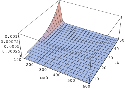
Figure 2: $\Gamma(h^{0}\to b\bar{s}+s\bar{b})$ in GeV as a function of ($\tan\beta$, $m_{A}$ (GeV)).

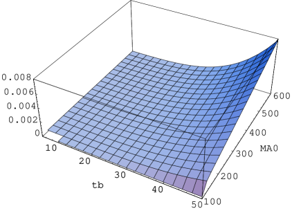
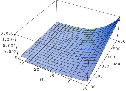
Figure 3: $\Gamma(H^{0}\to b\bar{s}+s\bar{b})$ and $\Gamma(A^{0}\to b\bar{s}+s\bar{b})$ in GeV as a function of ($\tan\beta$, $m_{A}$ (GeV)).

In Figs. 2 through 4, the MSSM parameters have been grouped into pairs ($\tan\beta$, $m_{A}$) and ($M_{2}$, $A$) in order to visualize the individual dependences of the FCHD widths for each neutral Higgs boson. Figs. 2 and  3 show $\Gamma(h^{0}\to b\bar{s}+s\bar{b})$, $\Gamma(H^{0}\to b\bar{s}+s\bar{b})$ and $\Gamma(A^{0}\to b\bar{s}+s\bar{b})$ as functions of the pair ($\tan\beta$, $m_{A}$). A common clear behaviour of all three decay widths is the increase with $\tan\beta$, yielding maximal FC effects at large $\tan\beta$ values. In the rest of the numerical analysis we have chosen $\tan\beta=35$, as specified in (4). Notice that the behaviour for the $A^{0}$ decay is indistinguishable from the $H^{0}$ case.

The behaviour with $m_{A}$ is less uniform. As one can see from Figs. 2 and 3, the decay widths $\Gamma(H^{0}\to b\bar{s}+s\bar{b})$ and $\Gamma(A^{0}\to b\bar{s}+s\bar{b})$ clearly increase with $m_{A}$ owing to obvious phase space effects, i.e. increasing phase space for larger Higgs-boson masses. In contrast, $\Gamma(h^{0}\to b\bar{s}+s\bar{b})$ shows a less obvious dependence on $m_{A}$. For small values of $m_{A}$ and large $\tan\beta$ we see a sharp decrease of the decay width with $m_{A}$. This is due to the fact that $|\sin\alpha|$ decreases rapidly between $m_{A}=100$ and 130 GeV and this decrease strongly affects the self-energy–like diagrams, which are proportional to $\sin\alpha$ (see analytical formulas). Since the mass of the lightest Higgs boson $h^{0}$ reaches a constant value and the $m_{A}$-dependence of $\sin\alpha$ is weak for large values of $m_{A}$, the decay width is very flat in this range.

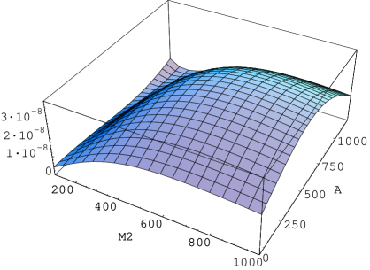
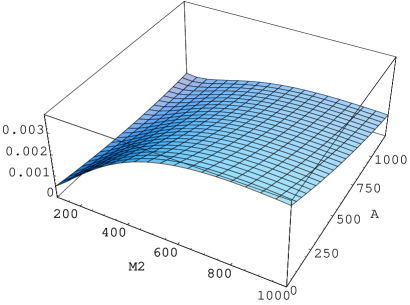
Figure 4: $\Gamma(h^{0}\to b\bar{s}+s\bar{b})$ and $\Gamma(H^{0}\to b\bar{s}+s\bar{b})$ in GeV as a function of ($M_{2}$ (GeV), $A$ (GeV)).

Fig. 4 shows the behaviour of the decay widths with respect to ($M_{2}$, $A$). Since the behaviour for the $A^{0}$ decay is indistinguishable from the $H^{0}$ case, we do not show the $A^{0}$ decay dependence from now on. Results for the $H^{0}$ decays are applied to this case directly. Clearly, for the heavy Higgs boson, the decay width grows with $M_{2}$ up to an approximately constant value and decreases with the trilinear parameter $A$. A less obvious behaviour appears for the $h^{0}$ case, depending on values of $M_{2}$, $A$ and the other MSSM parameters. In this case, we found a similar behaviour with respect to $M_{2}$, but in contrast to the previous case we now have an increase of the decay width with growing $A$ up to a maximum value and then a decrease with this parameter.

Now we focus on the behaviour with respect to the other MSSM parameters. First, in Fig. 5 we show the behaviour of the flavour-changing Higgs decays $\Gamma(H_{x}\to b\bar{s}+s\bar{b})$ $(H_{x}=h^{0}\,,H^{0})$ as functions of the $\mu$ parameter for three different values of $m_{A}$. The shaded regions in these figures correspond to the region excluded by LEP bounds on the chargino mass $|\mu|\lesssim 90$ GeV. We can see that the width for the $H^{0}$ decay is approximately symmetric under $\mu\to-\mu$, depending of the $m_{A}$ values. In contrast, the $\Gamma(h^{0}\to b\bar{s}+s\bar{b})$ width is more unsymmetric with respect to the sign of $\mu$. Note that all decay widths increase with $|\mu|$ for $|\mu|\lesssim 500$ GeV, then reach a maximum, and finally decrease. Regarding the behaviour at very small $\mu$ values, we have also found that the widths do not vanish at $\mu=0$. The origin of this comes entirely from contributions driven by electroweak gauge couplings.

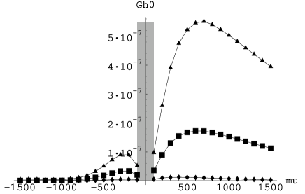
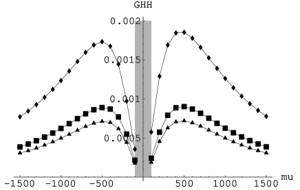
Figure 5: $\Gamma(H_{x}\to b\bar{s}+s\bar{b})$ $(H_{x}=h^{0},H^{0})$ in GeV as a function of $\mu$ (GeV). Lines with triangles, boxes, and diamonds correspond to $m_{A}=200$ GeV, $m_{A}=250$ GeV, and $m_{A}=400$ GeV respectively.

Figure 6: $\Gamma(H_{x}\to b\bar{s}+s\bar{b})$ as a function of $M_{0}$ (GeV). Other parameters as in (4).

Fig. 6 shows the behaviour of the $h^{0}$(left panel) and $H^{0}$ (right panel) decays as functions of the common soft SUSY-breaking squark-mass parameter $M_{0}$. The region below $M_{0}=425$ GeV implies too low and hence forbidden values for the squark masses. The $h^{0}$ decay width has a small value for light $M_{0}$ due to the fact that chargino and neutralino contributions have opposite sign there. For higher values of $M_{0}$, the neutralino contributions change sign and the partial cancellation disappears, therefore, the decay width increases until it reaches a maximum and then decreases for heavier squarks. The previously mentioned cancellation for small values of $M_{0}$ is less obvious for the heavy Higgs, the clearly visible effect is the decrease due to the growing squark masses. Notice that the decreasing behaviour is slower in this case.

In the following we study the behaviour of the corresponding FCHD with respect to $\lambda$. The MSSM parameters are again the ones chosen in (4). Given this set of parameters, the experimental lower bound on the squark masses restricts the allowed range of the mixing parameter to $0\leq\lambda\leq 0.93$. Figs. 7 and 8 contain the branching ratios and show the behaviour individually for the neutralino contributions (lines with diamonds), the chargino contributions (lines with stars), and the total SUSY-EW contributions (lines with boxes) up to the maximal allowed value of $\lambda$. For about $\lambda=0.8$, the branching ratio is around $3\times 10^{-5}$ for the lightest Higgs boson and $1.7\times 10^{-3}$ for $H^{0}$ and $A^{0}$. We remark that the SM value for this branching ratio is several orders of magnitude smaller, yielding $Br(H_{SM}\to b\bar{s}+s\bar{b})\sim 4\times 10^{-8}$ for $m_{H_{SM}}=114$ GeV. A similar result can be extracted from [29].

\psfrag{MA0}{$\,m_{A}$}\psfrag{tb}{{$\tan\beta$}}\psfrag{M2}{$\,M_{2}$}\psfrag{A}{{$A$}}\psfrag{GA0}{$\Gamma(A^{0}\rightarrow b\bar{s}+s\bar{b})$}\psfrag{GHH}{$\Gamma(H^{0}\rightarrow b\bar{s}+s\bar{b})$}\psfrag{Gh0}{$\Gamma(h^{0}\rightarrow b\bar{s}+s\bar{b})$}\psfrag{mu}{$\,\mu$}\psfrag{M0}{$\,M_{0}$}\psfrag{l}{$\lambda$}\psfrag{Brh0}{$Br(h^{0}\rightarrow b\bar{s}+s\bar{b})$}\psfrag{BrH0}{$Br(H^{0}\rightarrow b\bar{s}+s\bar{b})$}\includegraphics[height=130.88284pt,width=213.39566pt,clip={}]{fig7a.eps}

\psfrag{MA0}{$\,m_{A}$}\psfrag{tb}{{$\tan\beta$}}\psfrag{M2}{$\,M_{2}$}\psfrag{A}{{$A$}}\psfrag{GA0}{$\Gamma(A^{0}\rightarrow b\bar{s}+s\bar{b})$}\psfrag{GHH}{$\Gamma(H^{0}\rightarrow b\bar{s}+s\bar{b})$}\psfrag{Gh0}{$\Gamma(h^{0}\rightarrow b\bar{s}+s\bar{b})$}\psfrag{mu}{$\,\mu$}\psfrag{M0}{$\,M_{0}$}\psfrag{l}{$\lambda$}\psfrag{Brh0}{$Br(h^{0}\rightarrow b\bar{s}+s\bar{b})$}\psfrag{BrH0}{$Br(H^{0}\rightarrow b\bar{s}+s\bar{b})$}\includegraphics[height=130.88284pt,width=213.39566pt,clip={}]{fig7b.eps}

Figure 7: $Br(h^{0},H^{0}\to b\bar{s}+s\bar{b})$ versus $\lambda$ for the parameter set (4). Diamonds (stars) denote neutralino (chargino) contributions, boxes the total SUSY-EW contributions.

\psfrag{MA0}{$\,m_{A}$}\psfrag{tb}{{$\tan\beta$}}\psfrag{M2}{$\,M_{2}$}\psfrag{A}{{$A$}}\psfrag{GA0}{$\Gamma(A^{0}\rightarrow b\bar{s}+s\bar{b})$}\psfrag{GHH}{$\Gamma(H^{0}\rightarrow b\bar{s}+s\bar{b})$}\psfrag{Gh0}{$\Gamma(h^{0}\rightarrow b\bar{s}+s\bar{b})$}\psfrag{mu}{$\,\mu$}\psfrag{M0}{$\,M_{0}$}\psfrag{l}{$\lambda$}\psfrag{Brh0}{$Br(h^{0}\rightarrow b\bar{s}+s\bar{b})$}\psfrag{BrH0}{$Br(H^{0}\rightarrow b\bar{s}+s\bar{b})$}\includegraphics[width=213.39566pt,height=130.88284pt,clip={}]{fig8a.eps}

\psfrag{MA0}{$\,m_{A}$}\psfrag{tb}{{$\tan\beta$}}\psfrag{M2}{$\,M_{2}$}\psfrag{A}{{$A$}}\psfrag{GA0}{$\Gamma(A^{0}\rightarrow b\bar{s}+s\bar{b})$}\psfrag{GHH}{$\Gamma(H^{0}\rightarrow b\bar{s}+s\bar{b})$}\psfrag{Gh0}{$\Gamma(h^{0}\rightarrow b\bar{s}+s\bar{b})$}\psfrag{mu}{$\,\mu$}\psfrag{M0}{$\,M_{0}$}\psfrag{l}{$\lambda$}\psfrag{Brh0}{$Br(h^{0}\rightarrow b\bar{s}+s\bar{b})$}\psfrag{BrH0}{$Br(H^{0}\rightarrow b\bar{s}+s\bar{b})$}\includegraphics[width=213.39566pt,height=130.88284pt,clip={}]{fig8b.eps}

Figure 8: Same as in Fig. 7, for $0<\lambda<0.4$.

Investigating the contributions from charginos and neutralinos separately, we found that the neutralino contribution increases monotonically with $\lambda$, being exactly zero for $\lambda=0$, as expected. On the other hand, the contributions from charginos show explicitly the two FC sources, CKM and quark-squark misalignment. In fact, the chargino contribution is different from zero for $\lambda=0$. The non-zero value at $\lambda=0$ is due to CKM mixing which is not present in neutralino (or gluino) loops. The CKM effect and the effect of squark mixing for small $\lambda\neq 0$ partially cancel each other, leading to a minimum around $\lambda=0.2$. This minimum depends strongly on the particular input for the SUSY mass parameters. For larger values of $\lambda$ the non-CKM flavour-mixing effect dominates and the branching ratio increases, due to a change of sign in $F_{L}^{(x)}$ after the minimum. For our choice for the SUSY mass parameters, eq. (4), the total neutralino contribution to the form factors, $F_{L}$ and $F_{R}$, is negative for all the studied values of $\lambda$, but for the chargino contribution $F_{R}$ is always positive and $F_{L}$ changes sign, being positive for values of $\lambda\leq 0.2$ and negative for the rest of the studied $\lambda$ values. To illustrate this more explicitly, we show in Fig.8 the branching ratios as function of $\lambda$ for the range of small $\lambda$ below 0.4. The constructive interference of both neutralino and chargino terms lead to a multiple enhancement of the individual contributions in the decay rates.

We notice also that $|F_{L}|$ is larger than $|F_{R}|$ for both, chargino and neutralino contributions. It is also expected since the dominant FC effect enters through the $LL$ entry of the squark mass matrix. Regarding the size of the total chargino/neutralino contributions and which diagram is the dominant one, they depend in general on the particular Higgs boson and the other MSSM parameters and again on the value of $\lambda$. In particular, for $\lambda=0.5$, we find that the total chargino and neutralino contributions are of the same order, with the chargino contribution being slightly larger. These comments apply to all three Higgs bosons. Finally, for $0.15<\lambda<0.4$ the total contribution from neutralinos dominates that from charginos, also for the three Higgs bosons (see Fig. 8). However, the behavior at very small $\lambda$ values is opposite to the previous one, and it is in agreement with the results from the effective Lagrangian approach which incorporates the mass insertion approximation [18].

\psfrag{MA0}{$\,m_{A}$}\psfrag{tb}{{$\tan\beta$}}\psfrag{M2}{$\,M_{2}$}\psfrag{A}{{$A$}}\psfrag{GA0}{$\Gamma(A^{0}\rightarrow b\bar{s}+s\bar{b})$}\psfrag{GHH}{$\Gamma(H^{0}\rightarrow b\bar{s}+s\bar{b})$}\psfrag{Gh0}{$\Gamma(h^{0}\rightarrow b\bar{s}+s\bar{b})$}\psfrag{mu}{$\,\mu$}\psfrag{M0}{$\,M_{0}$}\psfrag{l}{$\lambda$}\psfrag{Brh0}{$Br(h^{0}\rightarrow b\bar{s}+s\bar{b})$}\psfrag{BrH0}{$Br(H^{0}\rightarrow b\bar{s}+s\bar{b})$}\includegraphics[width=213.39566pt,height=130.88284pt,clip={}]{fig9.eps}

Figure 9: $Br(h^{0}\to b\bar{s}+s\bar{b})$ as a function of $\lambda$ for $m_{A}=150$ GeV (line with diamonds), $m_{A}=200$ GeV (line with stars) and $m_{A}=250$ GeV (line with boxes).

The results in Fig. 7 and Fig. 8 are for $m_{A}=400$ GeV. We want to emphasize that the decay rates of $h^{0}$ are much larger for smaller values of $m_{A}$ (see Fig. 2) and therefore yield larger values of the branching ratio $Br(h^{0}\to b\bar{s}+s\bar{b})$, e.g. $Br(h^{0}\to b\bar{s}+s\bar{b})\simeq 2\times 10^{-3}$ for $m_{A}=150$ GeV and $\lambda=0.85$. To illustrate the $m_{A}$ dependence, we show in Fig. 9 the results for this branching ratio as a function of $\lambda$ for $m_{A}=150\,,200\,,250$ GeV. Large branching ratios are found for small $m_{A}$ and large $\lambda$ values.

In summary, the FCHD branching ratios that we have found in this section are quite sizable, and are in fact some orders of magnitude larger than the corresponding SM rates, but small in comparison with the SUSY-QCD contributions computed previously in [16]. There are, however, important interference terms, which modify the SUSY-QCD effects remarkably. The combined results for the SUSY-EW, SUSY-QCD and the total contributions to the $Br(H_{x}\to b\bar{s}+s\bar{b})$ $H_{x}=(h^{0},H^{0})$ are displayed as a function of $\lambda$ in Fig. 10. Note that the absolute value for gluino, chargino (above the minimum) and neutralino contributions grow with $\lambda$ separately. The SUSY-QCD quantum contributions are at least one order of magnitude larger than the pure SUSY-EW contributions. However, these later contribute with opposite sign, providing an important interference effect.

Figure 10: SUSY-EW (Diamonds), SUSY-QCD (stars) and total (boxes) contributions to the $Br(H_{x}\to b\bar{s}+s\bar{b})$ $H_{x}=(h^{0},H^{0})$ as a function of $\lambda$ for the selected MSSM parameters.

5 Non-decoupling behaviour of heavy SUSY particles

In this section we study the non-decoupling behaviour of squarks, charginos and neutralinos of the SUSY-EW contributions to FCHD into $b\bar{s}$ and $s\bar{b}$. This non-decoupling behaviour of the SUSY particles also happens in the SUSY-QCD contributions [16] and means that the FC effects remain non-vanishing even in the most pessimistic scenario of a very heavy SUSY spectrum. The motivation to analyze these effects, including both the SUSY-EW and the SUSY-QCD contributions, is that they could provide a very efficient way to search for indirect SUSY signals at next generation colliders.

The origin of this non-decoupling behaviour in the SUSY-EW contributions is, as in the SUSY-QCD case, the fact that the mass suppression induced by the heavy-particle propagators is compensated by the mass parameter factors coming from the interaction vertices, this being generic in Higgs–boson physics. It has been previously analyzed at length in the case of flavour-preserving MSSM Higgs decays [30, 31, 32, 33, 34]. The non-decoupling contributions to effective FC Higgs Yukawa couplings have also been studied in the effective-Lagrangian approach for the quark sector [18, 17] and the leptonic sector [35]. In this approach, the FC effects are encoded in a set of nonholomorphic dimension-four effective operators which appear due to SUSY breaking induced from the radiative corrections. It usually considers just the dominant contributions that come from large Yukawa couplings and assumes large $\tan\beta$ values. It is simple, but can not easily implement $SU(2)\times U(1)$ electroweak symmetry breaking effects which are relevant for small values of $\tan\beta$. We will use here instead the full diagrammatic approach which has the advantage of taking into account all EW loop contributions and is valid for all $\tan\beta$ values. Since, on the other hand, we are not using the mass–insertion approximation, our results are more general, being valid for all values of the FC parameter $\lambda$. We will see that our results converge in the large $\tan\beta$ limit and for small $\lambda$ values to the mass insertion approximation results of the effective Lagrangian approach.

In order to show analytically the non-decoupling behaviour of squarks, charginos and neutralinos in the FCHD, we perform a systematic expansion of the form factors involved, and hence of the partial widths, in inverse powers of the heavy SUSY masses and look for the first term in this expansion. We have considered the simplest hypothesis for the SUSY masses where all the soft breaking squark mass parameters, collectively denoted by $M_{0}$, the $\mu$ parameter, the trilinear parameters, collectively denoted by $A$ and the gaugino masses, are chosen to be of the same order and much greater than the electroweak scale $M_{EW}$,

$$M_{S}\sim M_{0}\sim M_{\tilde{g}}\sim M_{1}\sim M_{2}\sim\mu\sim A\gg M_{EW},$$ (5.1)

where $M_{0}=M_{\tilde{Q}}=M_{\tilde{U}}=M_{\tilde{D}}$ and $M_{\tilde{g}}$ is the gluino mass. The bino and wino soft-breaking masses, $M_{1}$ and $M_{2}$, are chosen in our numerical evaluations to follow the GUT relations, $M_{1}=\gamma M_{\tilde{g}}$ and $M_{2}=\eta M_{\tilde{g}}$, with $\gamma=\frac{5}{3}\frac{g_{1}^{2}}{g_{3}^{2}}$ and $\eta=\frac{g^{2}}{g_{3}^{2}}$. In order to provide more compact analytical results that can be easily used for future phenomenological studies, we have also analyzed the case of equal SUSY mass parameters, $M_{S}=M_{0}=M_{\tilde{g}}=M_{1}=M_{2}=\mu=A$, where $\gamma=\eta=1$.

In this section, we present the expansions of the SUSY-EW contributions to the form factors in inverse powers of $M_{S}$ and keep just the leading contribution of this expansion by considering that all the remaining involved mass scales $m_{H^{0}},m_{A},m_{h^{0}},m_{Z},m_{W}$ and $m_{q}$ are of order $M_{EW}$. To this end, we use the results of the expansions of the one-loop functions and of the rotation matrices that are given in Appendix B. In the general case of arbitrary $\gamma$ and $\eta$, we find the analytical results for the various contributions coming from chargino-squark and neutralino-squark loops that are collected in Appendix C. We next comment these results. First, we can see from eqs.(C.1) to (C.7) that, taking all SUSY mass parameters arbitrarily large and of the same order, ${\cal O}(M_{S})$, the SUSY-EW contributions to the form factors lead to a non-zero value. That is, they do not decouple in the large SUSY mass scenario. Regarding the ultraviolet behaviour, we have checked that the various contributions shown in formulas (C.1) to (C.7) are separately finite. A discussion on the relative signs and the sizes of chargino and neutralino contributions to the form factors, $F_{L}$ and $F_{R}$, is already included in the previous section. In general, the approximate analytical results show similar features than the exact results.

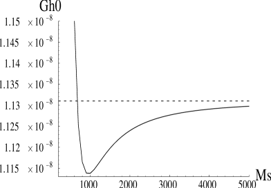
Figure 11: Non-decoupling behaviour of $\Gamma(H_{x}\to b\bar{s}+s\bar{b})$ in GeV with $M_{0}=\mu=A=M_{\tilde{g}}=M_{S}$, $M_{1}=\frac{5}{3}\frac{g_{1}^{2}}{g_{3}^{2}}M_{\tilde{g}}$ and $M_{2}=\frac{g^{2}}{g_{3}^{2}}M_{\tilde{g}}$, for $H_{x}=h^{0}$ (left panel) and $H_{x}=H^{0}$ (right panel) and for $\tan\beta=35$, $\lambda=0.5$, $m_{A}=m_{H^{0}}=250$ GeV and $m_{h^{0}}=135$ GeV. Exact one-loop results in solid lines and expansions given in eq. (C.1) in dashed lines are plotted for comparison.

In the following we show graphically some of these features. For definiteness, in all these plots we choose $M_{0}=M_{\tilde{g}}=\mu=A=M_{S}$, $M_{1}=\frac{5}{3}\frac{g_{1}^{2}}{g_{3}^{2}}M_{S}$, $M_{2}=\frac{g^{2}}{g_{3}^{2}}M_{S}$, $\tan\beta=35$ and, in order to simplify the analysis, we fix the Higgs boson masses to the following particular values, $m_{h^{0}}=135$ GeV, $m_{H^{0}}=250$ GeV and $m_{A}=250$ GeV. The non-decoupling behaviour of $\Gamma(H_{x}\to b\bar{s}+s\bar{b})$, for $H_{x}=h^{0}$ (left panel) and $H_{x}=H^{0}$ (right panel), as a function of $M_{S}$ is illustrated in Fig. 11. Here we have fixed $\lambda=0.5$. The exact one-loop results (solid lines) and the approximate large $M_{S}$ analytical expansions of eqs. (C.1) to (C.7) (dashed lines) are shown for comparison. The behaviour of $\Gamma(A^{0}\to b\bar{s}+s\bar{b})$ is practically identical to that of $\Gamma(H^{0}\to b\bar{s}+s\bar{b})$ and is not shown for brevity. We can see in these figures that, for large values of $M_{S}$, the exact partial widths tend to a non-vanishing value, characteristic of the non-decoupling behaviour, which is very well described by our asymptotic results. Notice that a proper study of the non-decoupling behaviour requires to take the input Higgs boson parameters, i.e the masses and the $\alpha$ mixing angle, at their tree level values. However, for illustrative purposes in the case of the lightest Higgs boson, we have prefered not to use the less phenomenologically appealing tree level value but to take instead an effective input mass value of 135 GeV which includes roughly the leading one-loop corrections for $\tan\beta=35\,,m_{A^{0}}=250$ GeV and $M_{S}\sim O(1TeV)$. Notice also that $M_{S}$ has been taken up to very large values just to illustrate the non-decoupling behaviour, but the convergence of the exact result to the asymptotic one is very good already at moderate $M_{SUSY}$ values (say $\geq 600$ GeV), what makes our asymptotic formulas useful for future phenomenological Higgs boson studies.

Figure 12: $\Gamma(H_{x}\to b\bar{s}+s\bar{b})$ as a function of $\lambda$. Left panel shows the $h^{0}$ decay and right panel corresponds with the $H^{0}$ decay. Exact one-loop chargino contribution in solid lines. The largest contribution corresponds to the effect coming only from misalignment; in the other, both possible effects are included. The neutralino contribution in dots. The expansions given in eq. (C.1 to C.7) in dashed lines are plotted for comparison. The fixed parameters are taken as in Fig. 11.

The dependence of the total chargino and neutralino contributions on the FC parameter $\lambda$ are shown in Fig. 12. Here we have fixed $M_{S}=1000$ GeV. The four lower lines take into account the two FC effects, quark mixing from off-diagonal terms in the CKM matrix and squark mixing from quark–squark misalignment, and show the comparative size of neutralino and chargino contributions. The solid (dotted) lower line is the total exact chargino (neutralino) contribution. The dashed lower lines are the corresponding approximate results given by our asymptotic formulas of Appendix C. First, we see that our asymptotic formulas describe extremely well the behavior with the $\lambda$ parameter for the whole studied interval, $0\leq\lambda\leq 1$, and this is true for both chargino and neutralino contributions. Second, the neutralino and chargino contributions behave as expected at very small $\lambda$ values. As has been already discussed in section 4, the chargino contributions are larger than the neutralino ones at these small $\lambda$ values, and at $\lambda=0$ the first one is non-vanishing whereas the second one vanishes. For larger $\lambda$ values the situation is different. Here we find that for $0.2\leq\lambda\leq 0.7$ the neutralino contribution is larger than the chargino contribution, which has now a minimum at about 0.4, and for $\lambda\geq 0.7$ again the chargino contribution dominates. As has been mentioned in section 4, the localization of this minimum varies with the choice of MSSM parameters. Notice that for moderate and large $\lambda$ values the alternative and more frequently used mass insertion approximation fails. It is clear from our plots that for these $\lambda$ values to assume a linear behaviour with $\lambda$ in the form factors is not correct and indeed can give a wrong conclusion on selecting the dominant contributions.

The two upper lines in Fig. 12 are the chargino contributions for the simplified case of $V_{CKM}=1$, which means that the only source of FC effects in this case is quark–squark misalignment. We see that the contribution vanishes at $\lambda=0$, as expected. Again the solid line is the exact result and the dashed line is the approximate asymptotic result. As in the previous case, we see the excellent agreement of our large $M_{S}$ results with the exact ones for all $\lambda$ values. The interesting feature here is to compare these lines with the previous ones and to notice how large is the effect of misalignment as compared to CKM in the chargino contributions. Indeed, we see that, for $\lambda\geq 0.2$, these two effects enter with different signs and give a total chargino contribution that is considerably lower than if we switch off the effects from CKM. This reduction of the chargino contribution is what makes finally the two contributions, from charginos and neutralinos, to be of comparable size, and therefore to neglect the later is not a good approximation.

Finally, we present the results for the case where all SUSY mass parameters are equal. These are very simple formulas that, besides of being useful for future phenomenological studies, allow us to compare more easily our results with those of the effective Lagrangian approach. The separate results for the various contributing diagrams are given in eqs. (C.9) to (C.14) of Appendix C. The total chargino and neutralino contributions to the form factors for equal mass scales are then given by

$$F_{L_{\tilde{\chi}^{\pm}}}^{(x)}=\frac{\alpha_{EW}}{4\pi}\frac{m_{b}}{2m_{W}\cos\beta}\left[\frac{1}{8m_{W}^{2}\sin^{2}\beta}\left[\left(V_{{\scriptscriptstyle CKM}}^{tb}V_{{\scriptscriptstyle CKM}}^{cs}m_{c}^{2}+V_{{\scriptscriptstyle CKM}}^{cb}V_{{\scriptscriptstyle CKM}}^{ts}m_{t}^{2}\right)F(\lambda)\right.\right.$$

$$\left.+\left(V_{{\scriptscriptstyle CKM}}^{cb}V_{{\scriptscriptstyle CKM}}^{cs}m_{c}^{2}+V_{{\scriptscriptstyle CKM}}^{tb}V_{{\scriptscriptstyle CKM}}^{ts}m_{t}^{2}\right)J(\lambda)\right]-\frac{1}{4}\left[\left(V_{{\scriptscriptstyle CKM}}^{cb}V_{{\scriptscriptstyle CKM}}^{cs}+V_{{\scriptscriptstyle CKM}}^{tb}V_{{\scriptscriptstyle CKM}}^{ts}\right)J(\lambda)\right.$$

$$\left.\left.+\left(V_{{\scriptscriptstyle CKM}}^{cb}V_{{\scriptscriptstyle CKM}}^{ts}+V_{{\scriptscriptstyle CKM}}^{tb}V_{{\scriptscriptstyle CKM}}^{cs}\right)F(\lambda)\right]\right]\left(\sigma_{2}^{(x)}+\tan\beta\,\sigma_{1}^{(x)*}\right)\,,$$ (5.2)

$$F_{L_{\tilde{\chi}^{0}}}^{(x)}=-\frac{\alpha_{EW}}{4\pi}\frac{m_{b}}{2m_{W}\cos\beta}\left[\frac{1}{8}\left(1+\frac{5}{9}\tan^{2}\theta_{W}\right)\left(\sigma_{2}^{(x)}+\tan\beta\,\sigma_{1}^{(x)*}\right)\right]F(\lambda)\,,$$ (5.3)

where $\alpha_{EW}=\frac{g^{2}}{4\pi}$. The results for $F_{R}$ are like the previous ones but replacing $m_{b}\rightarrow m_{s}$, $m_{c}\rightarrow m_{t}$ and taking the complex conjugate. Notice that in eq. (5.2) we can see clearly the relative importance of the two FC effects, quark–squark misalignment and CKM, which are driven respectively by the two functions $F(\lambda)$ and $J(\lambda)$ whose values at the origin are given by $F(0)=0$ and $J(0)=2$. We can also learn from eqs. (5.2) and (5.3) about the relative size of the contributions from Yukawa couplings versus those from pure gauge couplings. For instance, for $\lambda=0.5$, $m_{A}=250$ GeV and $\tan\beta=35$, the contributions from pure gauge couplings are about $50\%$ of the ones from Yukawa couplings and of opposite sign.

On the other hand, if we keep just the contributions from Yukawa couplings and neglect the contributions from pure gauge couplings, only the first term in eq. (5.2), which goes with the quark masses, remains. If we now consider the large $\tan\beta$ limit and the small $\lambda$ limit of the previous result, take $V_{{\scriptscriptstyle CKM}}=1$, and use the linear approximation where $F(\lambda)\simeq-\frac{2}{3}\lambda$, we get,

$$F_{L}^{(x)}=-\frac{\alpha_{EW}}{4\pi}\frac{m_{b}}{2m_{W}\cos\beta}\left(\frac{m_{c}^{2}}{12m_{W}^{2}}\tan\beta\,\sigma_{1}^{(x)*}\right)\lambda\,,$$ (5.4)

which agrees with the result from the effective-Lagrangian approach [18].

Finally, we briefly comment on the interesting limit called decoupling limit where $m_{A}>>m_{EW}$, which corresponds to a Higgs sector with very heavy Higgs bosons except $h^{0}$. Notice that when $x=h^{0}$, the common factor, $(\sigma_{2}^{(x)}+\tan\beta\,\sigma_{1}^{(x)*})$ in eqs. (5.2) and (5.3) is $(\cos\alpha+\tan\beta\sin\alpha)$ which in this decoupling limit goes to zero. Therefore, the decoupling of the heavy particles indeed occur in this case and we recover the SM vanishing value, as expected.

6 Conclusions

In this work we have computed the SUSY-EW quantum effects to flavour-changing MSSM Higgs-boson decays into $b\bar{s}$ and $s\bar{b}$. We have used the full diagrammatic approach and therefore our results are valid for all $\tan\beta$ values and for all values of the flavour-mixing parameter $\lambda$. We analyzed in full detail the dependence of the FCHD partial widths, with all the relevant MSSM parameters and $\lambda$, and found that they are very sensitive to $\tan\beta$, $\mu$, and $\lambda$. The branching ratios grow with both $\tan\beta$ and $\lambda$ and reach quite sizable values in comparison with the SM ones, in the large $\tan\beta$ and $\lambda$ region. For instance, for $\tan\beta=35$, $m_{A}=400$ GeV and $\lambda=0.8$, we found branching ratios of $3\times 10^{-5}$ for the $h^{0}$ and $1.7\times 10^{-3}$ for the $A^{0}$ and $H^{0}$. These SUSY-EW contributions are subdominant with respect to the SUSY-QCD contributions, but they contribute with opposite sign and important interference effects, which modify the SUSY-QCD effects remarkably, appear.

The most interesting feature of these SUSY-EW radiative contributions is their non-decoupling behaviour for large values of the SUSY particle masses. We have analyzed this behaviour in great detail and found that these SUSY-EW contributions to the FCHD widths, as the SUSY-QCD ones, indeed do not vanish for asymptotically large SUSY mass parameters. We presented a set of analytical asymptotic results that can be of great utility for future phenomenological studies. These results are in agreement with the ones of the effective–Lagrangian approach in the large $\tan\beta$ and small $\lambda$ limit. However, we checked that, for moderate $\tan\beta$ and $\lambda$ values, some of the contributions which are usually neglected in the effective–Lagrangian approach can be sizable and, therefore, a realistic estimate of the branching ratios should rely better on the full diagrammatic approach. In particular, the contributions driven from pure gauge couplings should not be ignored for these moderate values.

In conclusion, the results presented in this work indicate that a phenomenological detailed study of the Higgs boson decays into $b\bar{s}$ and $s\bar{b}$ can be very efficient as an indirect method in the future search for supersymmetry.

Appendix A

Here are the abbreviations used in the analytical expressions for the form factors $F_{L,R}^{(x)}$ (3.2).

$$\kappa_{L1}^{x,\,\tilde{\chi}^{0}}=B_{L\alpha a}^{(b)}D_{Rab}^{(x)}E_{L\alpha b}^{(s)} \iota_{L1}^{x,\tilde{\chi}^{0}}=B_{R\alpha a}^{(b)}E_{L\beta a}^{(s)}$$

$$\kappa_{L2}^{x,\,\tilde{\chi}^{0}}=B_{R\alpha a}^{(b)}D_{Lab}^{(x)}E_{R\alpha b}^{(s)} \iota_{L2}^{x,\tilde{\chi}^{0}}=B_{L\alpha a}^{(b)}E_{R\beta a}^{(s)}$$

$$\kappa_{L3}^{x,\,\tilde{\chi}^{0}}=B_{R\alpha a}^{(b)}D_{Lab}^{(x)}E_{L\alpha b}^{(s)} \iota_{L3}^{x,\tilde{\chi}^{0}}=B_{L\alpha a}^{(b)}E_{L\beta a}^{(s)}$$

$$\kappa_{L4}^{x,\,\tilde{\chi}^{0}}=B_{L\alpha a}^{(b)}D_{Rab}^{(x)}E_{R\alpha b}^{(s)}$$

$$\kappa_{L5}^{x,\,\tilde{\chi}^{0}}=B_{R\alpha a}^{(b)}D_{Rab}^{(x)}E_{L\alpha b}^{(s)}$$

$$\kappa_{L6}^{x,\,\tilde{\chi}^{0}}=B_{L\alpha a}^{(b)}D_{Lab}^{(x)}E_{R\alpha b}^{(s)}$$

$$\kappa_{L7}^{x,\,\tilde{\chi}^{0}}=B_{L\alpha a}^{(b)}D_{Lab}^{(x)}E_{L\alpha b}^{(s)}$$

$$\Sigma_{L}^{\tilde{\chi}^{0}}(p^{2}) = -\frac{g^{2}}{16\pi^{2}}B_{1}(p^{2},m_{\tilde{\chi}_{a}^{0}}^{2},m_{\tilde{d}_{\alpha}}^{2})B_{R\,\alpha a}^{(b)}E_{L\,\alpha a}^{(s)}$$

$$m_{b}\Sigma_{Ls}^{\tilde{\chi}^{0}}(p^{2}) = \frac{g^{2}m_{\tilde{\chi}_{a}^{0}}}{16\pi^{2}}B_{0}(p^{2},m_{\tilde{\chi}_{a}^{0}}^{2},m_{\tilde{d}_{\alpha}}^{2})B_{L\,\alpha a}^{(b)}E_{L\,\alpha a}^{(s)}$$ (A.1)

The $\kappa_{R}^{x,\,\tilde{\chi}^{0}}$, $\iota_{R}^{x,\,\tilde{\chi}^{0}}$, $\Sigma_{R}^{\tilde{\chi}^{0}}$ can be obtained from $\kappa_{L}^{x,\,\tilde{\chi}^{0}}$, $\iota_{L}^{x,\,\tilde{\chi}^{0}}$, $\Sigma_{L}^{\tilde{\chi}^{0}}$ respectively by exchanging all indices $(L\leftrightarrow R)$.

For chargino contributions, the $\kappa^{x,\,\tilde{\chi}^{-}}$, $\iota^{x,\,\tilde{\chi}^{-}}$, $\Sigma^{\tilde{\chi}^{-}}$ can be obtained from the previous expressions for $\kappa^{x,\,\tilde{\chi}^{0}}$, $\iota^{x,\,\tilde{\chi}^{0}}$, $\Sigma^{\tilde{\chi}^{0}}$ by making the replacements $m_{\tilde{\chi}_{a}^{0}}\rightarrow m_{\tilde{\chi}_{i}^{-}}$, $m_{\tilde{d}_{\alpha}}\rightarrow m_{\tilde{u}_{\alpha}}$, $B^{(b)}\rightarrow A^{(b)}$, $E_{L}^{(s)}\rightarrow A_{R}^{(s)*}$, $E_{R}^{(s)}\rightarrow A_{L}^{(s)*}$, $D^{(x)}\rightarrow W^{(x)}$, $a\rightarrow i$, $b\rightarrow j$.

The remaining abbreviations are

$$A_{L\alpha j}^{(d)} = -\frac{m_{d}}{\sqrt{2}m_{W}cos\beta}U_{j2}^{*}\left[R_{1\alpha}^{(u)}V_{{\scriptscriptstyle CKM}}^{cd}+R_{3\alpha}^{(u)}V_{{\scriptscriptstyle CKM}}^{td}\right]\,\,\,\,(d=b,s)$$

$$A_{R\alpha j}^{(d)} = V_{j1}\left[R_{1\alpha}^{(u)}V_{{\scriptscriptstyle CKM}}^{cd}+R_{3\alpha}^{(u)}V_{{\scriptscriptstyle CKM}}^{td}\right]-\frac{m_{c}}{\sqrt{2}m_{W}sin\beta}V_{j2}R_{2\alpha}^{(u)}V_{{\scriptscriptstyle CKM}}^{cd}$$

$$- \frac{m_{t}}{\sqrt{2}m_{W}sin\beta}V_{j2}R_{4\alpha}^{(u)}V_{{\scriptscriptstyle CKM}}^{td}\,\,\,\,(d=b,s)$$

$$B_{L\alpha a}^{(b)} = \sqrt{2}\left[\frac{m_{b}}{2m_{W}cos\beta}N_{a3}^{*}R_{3\alpha}^{(d)}+\left[\frac{1}{3}sin\theta_{W}N_{a1}^{{}^{\prime}*}-\frac{sin^{2}\theta_{W}}{3cos\theta_{W}}N_{a2}^{{}^{\prime}*}\right]R_{4\alpha}^{(d)}\right]$$

$$B_{R\alpha a}^{(b)} = \sqrt{2}\left[\left(-\frac{sin\theta_{W}}{3}N_{a1}^{{}^{\prime}}-\frac{1}{cos\theta_{W}}(\frac{1}{2}-\frac{sin^{2}\theta_{W}}{3})N_{a2}^{{}^{\prime}}\right)R_{3\alpha}^{(d)}+\frac{m_{b}}{2m_{W}cos\beta}N_{a3}R_{4\alpha}^{(d)}\right]$$

$$E_{L\alpha a}^{(s)} = -\sqrt{2}\left[\left(\frac{sin\theta_{W}}{3}N_{a1}^{{}^{\prime}*}+\frac{1}{cos\theta_{W}}(\frac{1}{2}-\frac{sin^{2}\theta_{W}}{3})N_{a2}^{{}^{\prime}*}\right)R_{1\alpha}^{(d)*}-\frac{m_{s}}{2m_{W}cos\beta}N_{a3}^{*}R_{2\alpha}^{(d)\,*}\right]$$

$$E_{R\alpha a}^{(s)} = -\sqrt{2}\left[-\frac{m_{s}}{2m_{W}cos\beta}N_{a3}R_{1\alpha}^{(d)*}+\left(-\frac{1}{3}sin\theta_{W}N_{a1}^{{}^{\prime}}+\frac{sin^{2}\theta_{W}}{3cos\theta_{W}}N_{a2}^{{}^{\prime}}\right)R_{2\alpha}^{(d)*}\right]$$

$$W_{Lij}^{(x)} = \frac{1}{\sqrt{2}}\left(-\sigma_{1}^{(x)}U_{j2}^{*}V_{i1}^{*}+\sigma_{2}^{(x)}U_{j1}^{*}V_{i2}^{*}\right)$$

$$W_{Rij}^{(x)} = \frac{1}{\sqrt{2}}\left(-\sigma_{1}^{(x)}U_{i2}V_{j1}+\sigma_{2}^{(x)}U_{i1}V_{j2}\right)$$

$$D_{Lab}^{(x)} = \frac{1}{2cos\theta_{W}}\left[(sin\theta_{W}N_{b1}^{*}-cos\theta_{W}N_{b2}^{*})(\sigma_{1}^{(x)}N_{a3}^{*}+\sigma_{2}^{(x)}N_{a4}^{*})\right.$$

$$+ (sin\theta_{W}N_{a1}^{*}-cos\theta_{W}N_{a2}^{*})(\sigma_{1}^{(x)}N_{b3}^{*}+\sigma_{2}^{(x)}N_{b4}^{*})\left.\right]$$

$$D_{Rab}^{(x)} = D_{Lab}^{(x)*}$$

$$S_{L,q}^{(x)} = -\frac{m_{q}}{2m_{W}\cos\beta}\>\sigma_{1}^{(x)*}$$

$$S_{R,q}^{(x)} = S_{L,q}^{(x)*}$$ (A.2)

$$\textrm{where }\sigma_{1}^{(x)}=\begin{pmatrix}\sin\alpha&\\ -\cos\alpha&\\ i\sin\beta&\end{pmatrix},\;\;\sigma_{2}^{(x)}=\begin{pmatrix}\cos\alpha\\ \sin\alpha\\ -i\cos\beta\end{pmatrix}\textrm{ for }x=(h_{0},H_{0},A_{0})$$

correspondingly, and $N_{a1}^{{}^{\prime}}=N_{a1}\cos\theta_{W}+N_{a2}\sin\theta_{W}$, $N_{a2}^{{}^{\prime}}=-N_{a1}\sin\theta_{W}+N_{a2}\cos\theta_{W}$ . The Higgs-squark-squark couplings $g_{H_{x}\tilde{q}_{\alpha}\tilde{q}_{\beta}}$ in the physical basis are given in Appendix A of [16] for the up-type squarks and down-type squarks independently. The quantities $R^{(u)}$, $R^{(d)}$, N, U and V are the matrices diagonalizing the mass matrices of the up squarks, down squarks, neutralinos and charginos, respectively.

Appendix B

In this appendix we give the expressions required to compute the leading contribution to the FCHD partial widths in the large SUSY mass limit defined in Sect 5, where $M_{S}\sim M_{0}\sim M_{\tilde{g}}\sim M_{1}\sim M_{2}\sim\mu\sim A\gg M_{EW}$. For that purpose we first write the values of the squark, chargino and neutralino masses and their corresponding rotation matrices and then the formulae for the two- and three-point integrals needed.

• The expressions for the squark masses and rotation matrices, in the limit of large SUSY mass parameters and keeping just the leading contribution, are

  $$M_{\tilde{q}_{1}}^{2}\simeq M_{0}^{2}\,\,,\,\,M_{\tilde{q}_{2}}^{2}\simeq M_{0}^{2}\,,\,M_{\tilde{q}_{3}}^{2}\simeq M_{0}^{2}(1-\lambda)\,\,,\,\,M_{\tilde{q}_{4}}^{2}\simeq M_{0}^{2}(1+\lambda)$$ (B.1)

  $$R_{11}^{(d)}\simeq-R_{12}^{(d)}\simeq R_{43}^{(d)}\simeq R_{44}^{(d)}\simeq\frac{m_{b}}{\sqrt{2}\lambda M_{0}^{2}}(A-\mu\tan\beta)$$

  $$R_{13}^{(d)}\simeq R_{14}^{(d)}\simeq-R_{21}^{(d)}\simeq-R_{22}^{(d)}\simeq-R_{33}^{(d)}\simeq R_{34}^{(d)}\simeq-R_{41}^{(d)}\simeq R_{42}^{(d)}\simeq\frac{1}{\sqrt{2}}$$

  $$R_{24}^{(d)}\simeq-R_{23}^{(d)}\simeq R_{31}^{(d)}\simeq R_{32}^{(d)}\simeq\frac{m_{s}}{\sqrt{2}\lambda M_{0}^{2}}(A-\mu\tan\beta)$$ (B.2)

  and similar results for $R^{(u)}$ just replacing $b\to t$, $s\to c$ and $\tan\beta\to\cot\beta$.

• The expressions for the chargino and neutralino masses and rotation matrices, in the limit of large SUSY mass parameters can be found in [36]. To leading order these masses are $M_{\tilde{\chi}_{1}^{-}}\simeq M_{2}$, $M_{\tilde{\chi}_{2}^{-}}\simeq|\mu|$ and $M_{\tilde{\chi}_{1}^{o}}\simeq M_{1}$, $M_{\tilde{\chi}_{2}^{o}}\simeq M_{2}$, $M_{\tilde{\chi}_{3}^{o}}=M_{\tilde{\chi}_{4}^{o}}\simeq|\mu|$,

• In the large SUSY mass limit the two- and three-point one-loop integrals approach their corresponding values at zero external momenta, $C_{0,11,12}(m_{q}^{2},m_{H}^{2},m_{q^{\prime}}^{2};m_{1}^{2},m_{2}^{2},m_{3}^{2})\simeq C_{0,11,12}(0,0,0;m_{1}^{2},m_{2}^{2},m_{3}^{2})$ and $B_{0,1}(p^{2};m_{1}^{2},m_{2}^{2})\simeq B_{0}(0;m_{1}^{2},m_{2}^{2})$, and we write these later as,

  $$C_{0}(0,0,0;m_{1}^{2},m_{2}^{2},m_{3}^{2})=-\frac{1}{2m_{2}^{2}}f_{1}(R_{1},R_{2})$$

  $$C_{11}(0,0,0;m_{1}^{2},m_{2}^{2},m_{3}^{2})=\frac{1}{3m_{2}^{2}}f_{10}(R_{1},R_{2})$$

  $$C_{12}(0,0,0;m_{1}^{2},m_{2}^{2},m_{3}^{2})=\frac{1}{6m_{2}^{2}}f_{13}(R_{1},R_{2})$$

  $$B_{0}(0;m_{1}^{2},m_{2}^{2})=\Delta-log\frac{m_{2}^{2}}{\mu_{0}^{2}}+g_{1}(R_{1})$$

  $$B_{1}(0;m_{1}^{2},m_{2}^{2})=-\frac{1}{2}\Delta+\frac{1}{2}log\frac{m_{2}^{2}}{\mu_{0}^{2}}-g_{1}(R_{1})-g_{2}(R_{1}),$$ (B.3)

  where $m_{1}$, $m_{2}$, and $m_{3}$, represent generically the masses of the different particles inside the loops, $R_{1}=m_{1}/m_{2}$, $R_{2}=m_{1}/m_{3}$ and the explicit expressions for the functions $f_{i}$ and $g_{i}$ can be found in [30]. For the simplest case, where $R_{1}=R_{2}=1$, they are $f_{1}(1,1)=f_{10}(1,1)=f_{13}(1,1)=1$ and $g_{1}(1)=g_{2}(1)=0$.

Appendix C

In this appendix we present the expansions of the SUSY-EW contributions to the form factors in inverse powers of $M_{S}$ where $M_{S}\sim M_{0}\sim M_{\tilde{g}}\sim M_{1}\sim M_{2}\sim\mu\sim A\gg M_{EW}$ and keeping just the leading contribution. The following results are valid for the most general case of arbitrary $\lambda$, $\gamma$, $\eta$ and $\tan\beta$, where $\gamma$ and $\eta$ are defined by, $M_{1}=\gamma M_{\tilde{g}}$ and $M_{2}=\eta M_{\tilde{g}}$. The form factor is,

$$F_{L}^{(x)}=F_{L_{a_{C}}}^{(x)}+F_{L_{b_{C}}}^{(x)}+F_{L_{c_{C}+d_{C}}}^{(x)}+F_{L_{a_{N}}}^{(x)}+F_{L_{b_{N}}}^{(x)}+F_{L_{c_{N}+d_{N}}}^{(x)}\,,$$ (C.1)

where the contributions from the different diagrams ($a_{C,N}$, $b_{C,N}$, $c_{C,N}$, and $d_{C,N}$) are given respectively by,

$$F_{L_{a_{C}}}^{(x)}=\frac{g^{2}}{16\pi^{2}}\frac{m_{b}}{2m_{W}\cos\beta}\left[\frac{\sigma_{1}^{(x)*}}{4}\left[\left(V_{{\scriptscriptstyle CKM}}^{cb}V_{{\scriptscriptstyle CKM}}^{cs}+V_{{\scriptscriptstyle CKM}}^{tb}V_{{\scriptscriptstyle CKM}}^{ts}\right)\left(G(\lambda,\eta)+\lambda S(\lambda,\eta)\right)\right.\right.$$

$$\left.+\left(V_{{\scriptscriptstyle CKM}}^{cb}V_{{\scriptscriptstyle CKM}}^{ts}+V_{{\scriptscriptstyle CKM}}^{tb}V_{{\scriptscriptstyle CKM}}^{cs}\right)\left(S(\lambda,\eta)+\lambda G(\lambda,\eta)\right)\right]$$

$$-\frac{M_{2}\mu}{M_{S}^{2}}\frac{\sigma_{2}^{(x)}}{4}\left[\left(V_{{\scriptscriptstyle CKM}}^{cb}V_{{\scriptscriptstyle CKM}}^{cs}+V_{{\scriptscriptstyle CKM}}^{tb}V_{{\scriptscriptstyle CKM}}^{ts}\right)G(\lambda,\eta)\right.$$

$$\left.\left.+\left(V_{{\scriptscriptstyle CKM}}^{cb}V_{{\scriptscriptstyle CKM}}^{ts}+V_{{\scriptscriptstyle CKM}}^{tb}V_{{\scriptscriptstyle CKM}}^{cs}\right)S(\lambda,\eta)\right]{\phantom{\frac{\sigma_{1}^{(x)*}}{4}}}\right]$$ (C.2)

$$F_{L_{b_{C}}}^{(x)}=\frac{g^{2}}{16\pi^{2}}\frac{m_{b}}{2m_{W}\cos\beta}\frac{\mu(A\sigma_{2}^{(x)}+\mu\sigma_{1}^{(x)*})}{M_{S}^{2}}\,\frac{1}{8m_{W}^{2}\ \sin^{2}\beta}\left[\left(V_{{\scriptscriptstyle CKM}}^{cb}V_{{\scriptscriptstyle CKM}}^{ts}m_{t}^{2}\right.\right.$$

$$\left.\left.+V_{{\scriptscriptstyle CKM}}^{tb}V_{{\scriptscriptstyle CKM}}^{cs}m_{c}^{2}\right)F(\lambda)+\left(V_{{\scriptscriptstyle CKM}}^{cb}V_{{\scriptscriptstyle CKM}}^{cs}m_{c}^{2}+V_{{\scriptscriptstyle CKM}}^{tb}V_{{\scriptscriptstyle CKM}}^{ts}m_{t}^{2}\right)J(\lambda)\right]$$ (C.3)

$$F_{L_{c_{C}+d_{C}}}^{(x)}=-\frac{g^{2}}{16\pi^{2}}\frac{m_{b}}{2m_{W}\cos\beta}\sigma_{1}^{(x)*}\left[\frac{\mu\left(\mu-A\tan\beta\right)}{4\sin 2\beta m_{W}^{2}\tan\beta M_{S}^{2}}\left[\left(V_{{\scriptscriptstyle CKM}}^{tb}V_{{\scriptscriptstyle CKM}}^{cs}m_{c}^{2}\right.\right.\right.$$

$$\left.\left.+V_{{\scriptscriptstyle CKM}}^{cb}V_{{\scriptscriptstyle CKM}}^{ts}m_{t}^{2}\right)F(\lambda)+\left(V_{{\scriptscriptstyle CKM}}^{cb}V_{{\scriptscriptstyle CKM}}^{cs}m_{c}^{2}+V_{{\scriptscriptstyle CKM}}^{tb}V_{{\scriptscriptstyle CKM}}^{ts}m_{t}^{2}\right)J(\lambda)\right]$$

$$-\frac{1}{4\cos\beta(M_{2}^{2}-\mu^{2})}\left[\mu\left(M_{2}\sin\beta+\mu\cos\beta\right)\left[\left(V_{{\scriptscriptstyle CKM}}^{cb}V_{{\scriptscriptstyle CKM}}^{cs}+V_{{\scriptscriptstyle CKM}}^{tb}V_{{\scriptscriptstyle CKM}}^{ts}\right)F(\lambda)\lambda\right.\right.$$

$$\left.+\left(V_{{\scriptscriptstyle CKM}}^{cb}V_{{\scriptscriptstyle CKM}}^{ts}+V_{{\scriptscriptstyle CKM}}^{tb}V_{{\scriptscriptstyle CKM}}^{cs}\right)J(\lambda)\lambda\right]$$

$$+2M_{2}\left(M_{2}\cos\beta+\mu\sin\beta\right)\left[\left(V_{{\scriptscriptstyle CKM}}^{cb}V_{{\scriptscriptstyle CKM}}^{cs}+V_{{\scriptscriptstyle CKM}}^{tb}V_{{\scriptscriptstyle CKM}}^{ts}\right)L(\lambda,\eta)\right.$$

$$\left.\left.\left.+\left(V_{{\scriptscriptstyle CKM}}^{cb}V_{{\scriptscriptstyle CKM}}^{ts}+V_{{\scriptscriptstyle CKM}}^{tb}V_{{\scriptscriptstyle CKM}}^{cs}\right)P(\lambda,\eta)\right]\right]{\phantom{\frac{1}{4\mu}}}\right]$$ (C.4)

$$F_{L_{a_{N}}}^{(x)}=\frac{g^{2}}{16\pi^{2}}\frac{m_{b}}{2m_{W}\cos\beta}\left[\frac{\tan^{2}\theta_{W}}{24}\left(\left(S(\lambda,\gamma)+\lambda G(\lambda,\gamma)\right)\sigma_{1}^{(x)*}-\frac{M_{1}\mu}{M_{S}^{2}}\sigma_{2}^{(x)}S(\lambda,\gamma)\right)\right.$$

$$\left.+\frac{1}{8}\left(\left(S(\lambda,\gamma)+\lambda G(\lambda,\gamma)\right)\sigma_{1}^{(x)*}-\frac{M_{2}\mu}{M_{S}^{2}}\sigma_{2}^{(x)}S(\lambda,\eta)\right)\right]$$ (C.5)

$$F_{L_{b_{N}}}^{(x)}=-\frac{g^{2}}{16\pi^{2}}\frac{m_{b}}{2m_{W}\cos\beta}(A\sigma_{1}^{(x)*}+\mu\sigma_{2}^{(x)})\left[\frac{M_{1}}{2M_{S}^{2}}\frac{\tan^{2}\theta_{W}}{18}S(\lambda,\gamma)\right]$$ (C.6)

$$F_{L_{c_{N}+d_{N}}}^{(x)}=-\frac{g^{2}}{16\pi^{2}}\frac{m_{b}}{2m_{W}\cos\beta}\sigma_{1}^{(x)*}\left[\frac{\tan^{2}\theta_{W}}{12}M_{1}\left(-\frac{1}{\cos\beta(M_{1}^{2}-\mu^{2})}(M_{1}\cos\beta+\mu\sin\beta)P(\lambda,\gamma)\right.\right.$$

$$\left.+\frac{2}{3}\frac{\left(A-\mu\tan\beta\right)}{M_{S}^{2}}K(\lambda,\gamma)\right)-M_{2}\left(\frac{1}{4\cos\beta(M_{2}^{2}-\mu^{2})}(M_{2}\cos\beta+\mu\sin\beta)P(\lambda,\eta)\right)$$

$$\left.-\mu\left(\frac{1}{24\cos\beta}\left[\frac{3}{(M_{2}^{2}-\mu^{2})}(M_{2}\sin\beta+\mu\cos\beta)+\frac{\tan^{2}\theta_{W}}{(M_{1}^{2}-\mu^{2})}(M_{1}\sin\beta+\mu\cos\beta)\right]J(\lambda)\lambda\right)\right]$$

(C.7)

$F_{R}^{(x)}$ can be obtained by replacing all ($L\leftrightarrow R$), $m_{b}\leftrightarrow m_{s}$, $m_{t}\leftrightarrow m_{c}$, and taking the complex conjugate. The previous result of eq. (C.1) is valid for all $m_{A}$ and $\tan\beta$ values and keep all the involved quark masses, $m_{t}$, $m_{b}$, $m_{c}$ and $m_{s}$, different from zero. The different functions of $\lambda$ that appear in the above expressions and their behaviour in the $\eta\to 1$ and $\gamma\to 1$ limits are given by,

$$F(\lambda) = \frac{2}{\lambda^{2}}[(\lambda+1)\ln(\lambda+1)+(\lambda-1)\ln(1-\lambda)-2\lambda];\,\,\lim_{\lambda\to 0}F(\lambda)\simeq-\frac{2\lambda}{3}-\frac{\lambda^{3}}{5},$$

$$J(\lambda) = \frac{2}{\lambda^{2}}[(\lambda+1)\ln(\lambda+1)-(\lambda-1)\ln(1-\lambda)];\,\,\lim_{\lambda\to 0}J(\lambda)\simeq 2+\frac{\lambda^{2}}{3},$$

$$S(\lambda,\eta) = f_{1}\left(\sqrt{1+\lambda},\frac{\sqrt{1+\lambda}}{\eta}\right)-f_{1}\left(\sqrt{1-\lambda},\frac{\sqrt{1-\lambda}}{\eta}\right);\,\,S(\lambda,1)=F(\lambda),$$

$$G(\lambda,\eta) = f_{1}\left(\sqrt{1+\lambda},\frac{\sqrt{1+\lambda}}{\eta}\right)+f_{1}\left(\sqrt{1-\lambda},\frac{\sqrt{1-\lambda}}{\eta}\right);\,\,G(\lambda,1)=J(\lambda),$$

$$L(\lambda,\eta) = -\ln(1+\lambda)-\ln(1-\lambda)+g_{1}\left(\frac{\eta}{\sqrt{1+\lambda}}\right)+g_{1}\left(\frac{\eta}{\sqrt{1-\lambda}}\right);\,\,L(\lambda,1)=-\frac{F(\lambda)\lambda}{2},$$

$$P(\lambda,\eta) = -\ln(1+\lambda)+\ln(1-\lambda)+g_{1}\left(\frac{\eta}{\sqrt{1+\lambda}}\right)-g_{1}\left(\frac{\eta}{\sqrt{1-\lambda}}\right);\,\,P(\lambda,1)=-\frac{J(\lambda)\lambda}{2},$$

$$K(\lambda,\eta) = \frac{1}{\lambda}\left(L(\lambda,\eta)-2g_{1}(\eta)\right);\,\,K(\lambda,1)=-\frac{F(\lambda)}{2}\,.$$ (C.8)

In the following we present our results for equal SUSY mass parameters. The contributions from charginos are,

$$F_{L_{a_{C}}}^{(x)}=\frac{g^{2}}{16\pi^{2}}\frac{m_{b}}{2m_{W}\cos\beta}\left[\frac{\sigma_{1}^{(x)*}}{4}\left[\left(V_{{\scriptscriptstyle CKM}}^{cb}V_{{\scriptscriptstyle CKM}}^{cs}+V_{{\scriptscriptstyle CKM}}^{tb}V_{{\scriptscriptstyle CKM}}^{ts}\right)\left(J(\lambda)+\lambda F(\lambda)\right)\right.\right.$$

$$\left.+\left(V_{{\scriptscriptstyle CKM}}^{cb}V_{{\scriptscriptstyle CKM}}^{ts}+V_{{\scriptscriptstyle CKM}}^{tb}V_{{\scriptscriptstyle CKM}}^{cs}\right)\left(F(\lambda)+\lambda J(\lambda)\right)\right]$$

$$-\frac{\sigma_{2}^{(x)}}{4}\left[\left(V_{{\scriptscriptstyle CKM}}^{cb}V_{{\scriptscriptstyle CKM}}^{cs}+V_{{\scriptscriptstyle CKM}}^{tb}V_{{\scriptscriptstyle CKM}}^{ts}\right)J(\lambda)\right.$$

$$\left.\left.+\left(V_{{\scriptscriptstyle CKM}}^{cb}V_{{\scriptscriptstyle CKM}}^{ts}+V_{{\scriptscriptstyle CKM}}^{tb}V_{{\scriptscriptstyle CKM}}^{cs}\right)F(\lambda)\right]{\phantom{\frac{\sigma_{1}^{(x)*}}{4}}}\right]$$ (C.9)

$$F_{L_{b_{C}}}^{(x)}=\frac{g^{2}}{16\pi^{2}}\frac{m_{b}}{2m_{W}\cos\beta}(\sigma_{2}^{(x)}+\sigma_{1}^{(x)*})\,\frac{1}{8m_{W}^{2}\sin^{2}\beta}\left[\left(V_{{\scriptscriptstyle CKM}}^{cb}V_{{\scriptscriptstyle CKM}}^{ts}m_{t}^{2}\right.\right.$$

$$\left.\left.+V_{{\scriptscriptstyle CKM}}^{tb}V_{{\scriptscriptstyle CKM}}^{cs}m_{c}^{2}\right)F(\lambda)+\left(V_{{\scriptscriptstyle CKM}}^{cb}V_{{\scriptscriptstyle CKM}}^{cs}m_{c}^{2}+V_{{\scriptscriptstyle CKM}}^{tb}V_{{\scriptscriptstyle CKM}}^{ts}m_{t}^{2}\right)J(\lambda)\right]$$ (C.10)

$$F_{L_{c_{C}+d_{C}}}^{(x)}=-\frac{g^{2}}{16\pi^{2}}\frac{m_{b}}{2m_{W}\cos\beta}\sigma_{1}^{(x)*}\left[\frac{\left(1-\tan\beta\right)}{8m_{W}^{2}\sin^{2}\beta}\left[\left(V_{{\scriptscriptstyle CKM}}^{tb}V_{{\scriptscriptstyle CKM}}^{cs}m_{c}^{2}\right.\right.\right.$$

$$\left.\left.+V_{{\scriptscriptstyle CKM}}^{cb}V_{{\scriptscriptstyle CKM}}^{ts}m_{t}^{2}\right)F(\lambda)+\left(V_{{\scriptscriptstyle CKM}}^{cb}V_{{\scriptscriptstyle CKM}}^{cs}m_{c}^{2}+V_{{\scriptscriptstyle CKM}}^{tb}V_{{\scriptscriptstyle CKM}}^{ts}m_{t}^{2}\right)J(\lambda)\right]$$

$$+\frac{1}{4}\left[\left(V_{{\scriptscriptstyle CKM}}^{cb}V_{{\scriptscriptstyle CKM}}^{cs}+V_{{\scriptscriptstyle CKM}}^{tb}V_{{\scriptscriptstyle CKM}}^{ts}\right)\left(\lambda F(\lambda)+J(\lambda)\left(1+\tan\beta\right)\right)\right.$$

$$\left.\left.+\left(V_{{\scriptscriptstyle CKM}}^{cb}V_{{\scriptscriptstyle CKM}}^{ts}+V_{{\scriptscriptstyle CKM}}^{tb}V_{{\scriptscriptstyle CKM}}^{cs}\right)\left(\lambda J(\lambda)+F(\lambda)\left(1+\tan\beta\right)\right)\right]{\phantom{\frac{\left(1-\tan\beta\right)}{8m_{W}^{2}}}}\right]$$ (C.11)

For neutralinos we get,

$$F_{L_{a_{N}}}^{(x)}=\frac{g^{2}}{16\pi^{2}}\frac{m_{b}}{2m_{W}\cos\beta}\left[\frac{1}{8}\left(1+\frac{\tan^{2}\theta_{W}}{3}\right)\left(\sigma_{1}^{(x)*}\left(F(\lambda)+\lambda J(\lambda)\right)-\sigma_{2}^{(x)}F(\lambda)\right)\right]$$ (C.12)

$$F_{L_{b_{N}}}^{(x)}=-\frac{g^{2}}{16\pi^{2}}\frac{m_{b}}{2m_{W}\cos\beta}\left[\frac{\tan^{2}\theta_{W}}{36}\left(\sigma_{1}^{(x)*}+\sigma_{2}^{(x)}\right)\right]F(\lambda)$$ (C.13)

$$F_{L_{c_{N}+d_{N}}}^{(x)}=-\frac{g^{2}}{16\pi^{2}}\frac{m_{b}}{2m_{W}\cos\beta}\sigma_{1}^{(x)*}\left[\frac{1}{8}\left(\frac{\tan^{2}\theta_{W}}{3}+1\right)\left(\lambda J(\lambda)+F(\lambda)\left(1+\tan\beta\right)\right)\right.$$

$$\left.-\frac{\tan^{2}\theta_{W}}{36}\left(1-\tan\beta\right)F(\lambda)\right]$$ (C.14)

References

• [1] S. L. Glashow, J. Iliopoulos, L. Maiani, Phys. Rev. D2, 1285 (1970).
• [2] H. E. Haber, G. L. Kane, Phys. Rept. 117, 75 (1985).
• [3] C. Hamzaoui, M. Pospelov, M. Toharia, Phys. Rev. D59, 095005 (1999), hep-ph/9807350; G. Isidori, A. Retico, JHEP 0111 (2001) 001, hep-ph/0110121.
• [4] A. J. Buras, P. H. Chankowski, J. Rosiek, L. Slawianowska, Nucl.Phys. B619 434 (2001), hep-ph/0107048; Phys. Lett. B546, 96 (2002); Nucl.Phys. B659, 3 (2003), hep-ph/0210145.
• [5] S. R. Choudhury, N. Gaur, Phys. Lett. B451, 86 (1999), hep-ph/9810307; K. S. Babu, C. F. Kolda, Rev. Lett. 84, 228 (2000), hep-ph/9909476; C.-S. Huang, L. Wei, Q.-S. Yan, S.-H. Zhu, Phys. Rev. D63, 114021 (2001) Erratum-ibid. D64 059902 (2001), hep-ph/0006250.
• [6] P. H. Chankowski, L. Slawianowska, Phys.Rev. D63, 054012 (2001), hep-ph/0008046.
• [7] C. Bobeth, T. Ewerth, F. Kruger, J. Urban, Phys.Rev. D64, 074014 (2001), hep-ph/0104284; Phys.Rev. D66 074021 (2002), hep-ph/0204225.
• [8] G. Isidori, A. Retico, JHEP 0209 (2002) 063, hep-ph/0208159.
• [9] M. A. Diaz, Phys. Lett. B304, 278 (1993), hep-ph/9303280; R. Garisto, J. N. Ng, Phys. Lett. B315, 372 (1993), hep-ph/9307301; F. M. Borzumati, Z. Phys. C63, 291 (1994), hep-ph/9310212; H. Baer, M. Brhlik, D. Castaño, X. Tata, Phys. Rev. D58, 015007 (1998), hep-ph/0009337; M. Carena, D. Garcia, U. Nierste, C. E. M. Wagner, Phys. Lett. B499 141 (2001), hep-ph/0010003.
• [10] S. Bertolini, F. Borzumati, A. Masiero, Phys. Lett. B192, 437 (1987); S. Bertolini, F. Borzumati, A. Masiero, G. Ridolfi, Nucl. Phys. B353, 591 (1991); R. Barbieri, G. F. Giudice, Phys. Lett. B309, 86 (1993), hep-ph/9303270; N. Oshimo, Nucl. Phys. B404, 20 (1993); Y. Okada, Phys. Lett. B315, 119 (1993), hep-ph/9307249.
• [11] V. D. Barger, M. S. Berger, P. Ohmann, R. J. Phillips, Phys. Rev. D 51 (1995) 2438, hep-ph/9407273.
• [12] G. Degrassi, P. Gambino, G. F. Giudice, JHEP 0012 (2000) 009, hep-ph/0009337.
• [13] For an extensive analysis of the phenomenological implications see, for instance: F. Gabbiani, E. Gabrielli, A. Masiero, L. Silvestrini, Nucl. Phys. B477, 321 (1996); M. Misiak, S. Pokorski, J. Rosiek, Adv. Ser. Direct. High Energy Phys. 15, 795 (1998).
• [14] M. Ciuchini, E. Franco, A. Masiero, L. Silvestrini, Phys. Rev. D 67 (2003) 075016 [Erratum-ibid. D 68 (2003) 079901, hep-ph/0212397.
• [15] M. Endo, M. Kakizaki, M. Yamaguchi, hep-ph/0311072.
• [16] A. M. Curiel, M. J. Herrero, D. Temes, Phys. Rev. D 67 (2003) 075008, hep-ph/0210335.
• [17] A. Dedes and A. Pilaftsis, Phys. Rev. D 67 (2003) 015012, hep-ph/0209306.
• [18] D. A. Demir, Phys. Lett. B571, 193 (2003), hep-ph/0303249.
• [19] M. E. Luke and M. J. Savage, Phys. Lett. B 307 (1993) 387, hep-ph/9303249; J. Guasch and J. Sola, Nucl. Phys. B 562 (1999) 3, hep-ph/9906268; C. F. Kolda, hep-ph/0003265; J. A. Aguilar-Saavedra and G. C. Branco, Phys. Lett. B 495 (2000) 347, hep-ph/0004190; S. Bejar, J. Guasch and J. Sola, Proc. of RADCOR 2000, ed. Howard E. Haber, hep-ph/0101294.
• [20] T. P. Cheng, M. Sher, Phys. Rev. D35, 3484 (1987).
• [21] K. Hikasa and M. Kobayashi, Phys. Rev. D36, 724 (1987); P. Brax and C. A. Savoy, Nucl. Phys. B447, 227 (1995), hep-ph/9503306.
• [22] W. Hollik, in Precision Tests of the Standard Electroweak Model, edited by P. Langacker (World Scientific, Singapore, 1995), pp. 37–116; Fortschr. Phys. 38, 165–260 (1990).
• [23] R. Mertig, M. Bohm, A. Denner, Comput. Phys. Commun.  64 (1991) 345; T. Hahn, C. Schappacher, Comput. Phys. Commun.  143 (2002) 54, hep-ph/0105349; T. Hahn, Comput. Phys. Commun.  140 (2001) 418, hep-ph/0012260; T. Hahn, M. Perez-Victoria, Comput. Phys. Commun.  118 (1999) 153, hep-ph/9807565.
• [24] Particle Data Group, K. Hagiwara et al., “Review of particle physics,” Phys. Rev. D66, 010001 (2002).
• [25] M. Acciarri et al. [L3 Collaboration], Phys. Lett. B 472 (2000) 420, hep-ex/9910007; G. Abbiendi et al. [OPAL Collaboration], Eur. Phys. J. C 14 (2000) 187 [Erratum-ibid. C 16 (2000) 707], hep-ex/9909051.
• [26] S. Heinemeyer, W. Hollik, G. Weiglein, Comput. Phys. Commun.  124 (2000) 76, hep-ph/9812320. FeynHiggs2.1beta is available on request. See also the web page:
http://wwwth.mppmu.mpg.de/members/heinemey/feynhiggs/FeynHiggs.html
• [27] R. Barate et al. [ALEPH Collaboration], Phys. Lett. B 429 (1998) 169; S. Ahmed et al. [CLEO Collaboration], hep-ex/9908022.
• [28] G. Belanger, F. Boudjema, A. Pukhov, A. Semenov, Comput. Phys. Commun.  149 (2002) 103, hep-ph/0112278.
• [29] G. Eilam, B. Haeri, A. Soni, Phys. Rev. D 41 875 (1990).
• [30] H. E. Haber, M. J. Herrero, H. E. Logan, S. Peñaranda, S. Rigolin, D. Temes, Phys. Rev. D 63 (2001) 055004, hep-ph/0007006; M. J. Herrero, S. Peñaranda, D. Temes, Phys. Rev. D 64 (2001) 115003, hep-ph/0105097.
• [31] R. A. Jiménez and J. Solà, Phys. Lett. B 389, 53 (1996), hep-ph/9511292; A. Bartl, H. Eberl, K. Hidaka, T. Kon, W. Majerotto and Y. Yamada, Phys. Lett. B 378, 167 (1996), hep-ph/9511385; H. Eberl, K. Hidaka, S. Kraml, W. Majerotto and Y. Yamada, Phys. Rev. D 62 (2000) 055006,hep-ph/9912463.
• [32] M.J. Herrero, Proceedings of the XXIX International Meeting on Fundamental Physics, Sitges, Barcelona, Spain, 5-9 Feb 2001. Editors V. Fonseca and A. Dobado, 319-342. Ed. CIEMAT 2001. hep-ph/0109291.
• [33] A. Dobado, M. J. Herrero, D. Temes, Phys. Rev. D65 075023 (2002), hep-ph/0107147; A. M. Curiel, M. J. Herrero, D. Temes, J. F. de Troconiz, Phys. Rev. D 65 075006 (2002), hep-ph/0106267.
• [34] J. Guasch, W. Hollik, S. Peñaranda, Phys. Lett. B 515, 367 (2001), hep-ph/0106027; hep-ph/0307012; M. Carena, H. E. Haber, H. E. Logan and S. Mrenna, Phys. Rev. D 65 (2002) 055005 [Erratum-ibid. D 65 (2002) 099902], hep-ph/0106116.
• [35] K. S. Babu and C. Kolda, Phys. Rev. Lett.  89 (2002) 241802, hep-ph/0206310; A. Dedes, J. R. Ellis and M. Raidal, Phys. Lett. B 549 (2002) 159, hep-ph/0209207; A. Brignole, A. Rossi, Phys. Lett. B566, 217 (2003), hep-ph/0304081.
• [36] J. F. Gunion, H. E Haber, Phys. Rev. D37, 2515 (1988).