Operator Product Expansion and Quark-Hadron Duality:
Facts and Riddles

Abstract

We review the status of the practical operator product expansion (OPE), when applied to two-point correlators of QCD currents which interpolate to mesonic resonances, in view of the violations of local quark-hadron duality. Covered topics are: a mini-review of mesonic QCD sum rules in vacuum, at finite temperature, or at finite baryon density, a comparison of model calculations of current-current correlation functions in 2D and 4D with the OPE expressions, a discussion of meson distribution amplitudes in the light of nonperturbatively nonlocal modifications of the OPE, and a reorganization of the OPE which (partially) resums powers of covariant derivatives.

1 Preface

We start by giving a short outline of the present review article:

In the next five sections we lay the foundations for reviewing (some of) the research on local quark-hadron duality violations being conducted within the last twenty years or so. We introduce the operator product expansion (OPE) as an expansion of a current-current correlator in powers of inverse Euclidean, external momenta and the strong coupling constant $\alpha_{s}$. We distinguish between the full OPE, which most probably is an asymptotic series, and truncations thereof used in practice. A definition of local quark-hadron duality, which conceptually rests on the OPE, is given. The concept of the OPE is applied to hadronic physics in the framework of the Shifman-Vainshtein-Zakharov (SVZ) sum rules associated with light- and heavy-quark mesons in vacuum and in a hot or baryon rich medium. We do not discuss the sum-rule program for baryonic resonances. We also review briefly the relation between power corrections and renormalons. Secs. 2 to 5 naturally have large overlaps with existing review articles and books on QCD sum rules and on theoretical as well as on practical aspects of the OPE [31, 50].

In Sec. 6 we take a closer look at violations of local duality. We first compare the predictions of analytically continued practical OPEs with the experimental data. Second, we review an instanton model calculation of the light-quark current-current correlator in Euclidean spacetime and compare the result with the practical OPE of this correlator. Third, we review an analysis of the current-current correlator in the ’t Hooft model. The focus is on oscillatory components in the decay width of heavy mesons (as a function of the meson mass) when taking $O(1/N_{c})$ corrections into account. The adopted point of view in the latter two investigations is that the model calculations are in some sense realistic, that is, they largely resemble the experimental situation. Disagreement between the prediction of hadronic spectra resting on the model calculation on the one hand and the OPE on the other hand thus are interpreted as violations of local quark-hadron duality. In Sec. 6.1 we give an overview on experimental hadron spectra induced by the electromagnetic current and by $\tau$ decays. We also address $B_{s}$-$\bar{B}_{s}$ mixing: a problem which can be tackled by appealing to local quark hadron duality. A rather large overlap of Sec. 6.2 and Sec. 6.3 with the reviews [32] exists. In the present review the analysis in the ’t Hooft model is presented in a more self-contained way than in [32].

A discussion of the effects of nonperturbative nonlocality in modified practical OPEs is carried out in section 7 of the review. In a first step the relation between power corrections in an OPE and mesonic distribution amplitudes is discussed. Subsequently, the theoretical and phenomenological need for the inclusion of nonlocal condensates is pointed out. We also review the systematic inclusion of nonperturbatively nonlocal quantities in the OPE-based description of the hadron-to-hadron, hadron-to-vacuum, and vacuum-to-vacuum matrix elements of time-ordered current-current products. Phenomenologically consequences are explored in the latter case. To the best of the author’s knowledge no review article exists which would have a substantial overlap with section 7.

The presentation is not very technical. Rather, we have tried to capture the basic theoretical concepts and their applications. Most of the time our discussion aims at a direct comparison with the experimental situation. This review is by no means complete – our apologies to all those authors whose contributions are not explicitly referred to.

2 Introduction

Quantum Chromodynamics (QCD), the non-Abelian gauge theory of interacting quarks and gluons, is by now the widely accepted microscopic theory of strong interactions. Embedded into the Standard Model of particle physics it has passed various experimental tests. The expansion about the situation of asympotically free fundamental degrees of freedom at large momenta or particle masses is a conceptually and practically appealing feature [1, 2, 3]. It has a wealth of applications: the perturbative calculability of the evolution of hadron structure functions [4, 5, 6, 7], a perturbative description of quark or gluon induced jets in $e^{+}e^{-}$ annihilations [8], the perturbative matching of the full theory to effective theories for heavy flavors [9, 10, 11, 12, 13, 14, 15, 16] and the matching of the electroweak sector of the Standard Model involving perturbative QCD corrections with a low-energy effective theory describing the weak decays and mixings of heavy flavors, see for example [17, 18] for $b\to s$ decays. Last but not least, at large external momenta asymptotic freedom guarantees the usefulness of an expansion of Euclidean correlation functions of hadron-interpolating currents starting from the parton model [19, 20]. This is crucial for the method of QCD sum rules [21, 22] whose explanation is the starting point of the present review.

While QCD is well understood and tested at large external momenta $p\gg 0.5\,$GeV the strongly coupled low-energy regime denies a perturbative treatment. The only presently known fundamental approach to learn about the dynamics of the relevant degrees of freedom populating the ground state of QCD at low energy and being responsible for the hadronic spectrum and hadron dynamics are lattice simulations [30]. Analytical approaches are not clear-cut – not even the identification of the relevant degrees of freedom is unique –, and explanations of low-energy phenomena have only been found partially so far. For example, the instanton [23] gas provides a plausible, microscopic mechanism for dynamical chiral symmetry breaking [25] and the large mass of the $\eta^{\prime}$ [125] but unless interactions between instantons are parametrized as in the instanton-liquid model (see [26] for a review) it does not explain color confinement. Dual models [27] based on the idea that confinement is realized through the dual Meissner effect [28, 29] explain confinement almost by definition and can not be considered fundamental.

QCD sum rules provide a successful analytic way to ’scratch’ into the nonperturbative regime. Many exhaustive reviews of the field exist [31], and therefore we will limit ourselves to a very basic introduction in the next section. The sum-rule approach is pragmatic in the sense that it does not aim at calculating nonperturbative ground-state parameters or hadronic wave functions from first principles. Rather, QCD sum rules extract universal nonperturbative parameters from limited experimental information to subsequently use them for predictions. The sum-rule method has been extended to investigate hadronic properties in the presence of a hot [74] or a dense hadronic medium (for a review see [108]) which is of great relevance for ongoing experiments with colliding (ultra)relativistic heavy ions.

The basic object of investigation in QCD sum rules is an $N$-point correlator of QCD currents. The sum-rule method rests on analyticity in the external momentum variable(s) and on the assumption of quark-hadron duality. In its strong, local form, quark-hadron duality is the situation that a hadronic cross section can be related pointwise to a theoretical expression obtained in terms of quark and gluon variables. At low energy strong limitations on the accuracy of the theoretical expression exist. One possible theoretical approach is the analytical continuation of the OPE [36] which is an asymptotic series in powers of the strong coupling $\alpha_{s}$ and in powers of the inverse external momentum $Q^{-1}$ (up to logarithms) [21, 142]. To circumvent the problem associated with the asymptotic series one appeals to analyticity in the external momentum variable to relate the incompletely known theoretical part to an average over the hadronic cross section by means of a dispersion relation [21]. This pragmatic approach is rather fruitful.

Different meanings are attributed to quark-hadron duality in the literature. For the present review, which is mainly concerned with its local form, we use the definition given by Shifman in [144] for a one-variable situation such as the $e^{+}e^{-}$ annihilation into hadrons. Shifman’s definition is as follows: The current correlator, associated with the process of hadron creation out of the vacuum, is theoretically evaluated in terms of quark and gluon fields at an external momentum $q$ with $q^{2}=-Q^{2}<0$ (Euclidean region) using an OPE [36]. Approximating this current correlator by a truncation of the purely perturbative part of the OPE at $\alpha_{s}^{k}$ and a truncation at power $Q^{-D}$ (not counting logarithms arising from anomalous dimensions of contributing operators), the uncertainty of the result should be of orders $\alpha_{s}^{(k+1)}$ and $Q^{-(D+1)}$ if the OPE represents a converging series. In practice one usually has $k=2$ or $k=3$ and $D=6$ or $D=8$ (practical OPE). The uncertainty in the truncated OPE would translate into an uncertainty of order $\alpha_{s}^{(k+1)}$ and $s^{-(D+1)/2}$ of the theoretically predicted spectral function $\rho_{\tiny{\mbox{theo}}}(s)$. The latter is obtained by calculating the imaginary part of a term-by-term analytical continuation to negative $Q^{2}$, $-Q^{2}\equiv s>0$, of the truncated OPE. If the experimentally measured spectral function $\rho_{\tiny{\mbox{exp}}}(s)$ coincides with $\rho_{\tiny{\mbox{theo}}}(s)$ up to the above uncertainty within a certain range of $s$ values we say that the quark-gluon prediction, resting on the OPE, is dual to the hadronic spectral function in this range. If this is not true we speak of a violation of local quark-hadron duality. While local quark-hadron duality is badly violated in practical OPEs at momenta close to the lowest resonance mass there usually is a window of Euclidean momenta $Q$ where the practical OPE is seen to be equal (or dual) to the dispersion integral over the spectral function. We will refer to this kind of duality as global or sum-rule duality. It is known for a long time that in some exceptional channels QCD sum rules do not work [38, 37, 39, 40]. Namely, a stability under the variation of quantities parametrizing our ignorance about the hadron spectrum and the vacuum structure does not exist in these channels.

3 SVZ sum rules

To prepare for the discussion of duality violation in later chapters we briefly review the method of QCD sum rules of Shifman, Vainshtein, and Zakharov (SVZ)[21, 22] focussing on mesonic two-point correlators. A remark on the notation is in order: In this and subsequent sections multiple meanings are attributed to the symbol $T$. It may stand for a correlator or time-ordering or the temperature. The symbol $\bar{T}$ is the inverse Borel transform of $B[T]$. What is meant should become clear from the context. We apologize for the inconvenience.

Let us start by giving a more specific characterization of the SVZ approach than in the last section: The idea is to express hadron parameters in terms of expectation values of gauge invariant operators which are composed of fundamental quark and/or gluon fields. In practice, the hadron parameters of the lowest states are studied. The lowest states are explicitly presented in models for the spectral functions. The higher resonances are absorbed into a continuum which is usually approximated by perturbative QCD. To separate the continuum from the lowest state an effective threshold $s_{0}$, which is a model parameter, is introduced. The parameter $s_{0}$ is to be determined by the sum rule by requiring hadron parameters to be least sensitive to its variation. Obviously, one does not assume local quark-hadron duality here - only the integral over the perturbative QCD spectrum is assumed to be equal to the integral over the experimental spectrum down to the threshold $s_{0}$.

The basic object of investigation is the vacuum correlator of two gauge invariant, hadron-interpolating currents $j_{L}^{F}$ and $j_{L^{\prime}}^{F^{\prime}}$ in momentum space where $L,L^{\prime}$ and $F,F^{\prime}$ denote Lorentz and flavor quantum numbers, respectively

$$T^{FF^{\prime}}_{LL^{\prime}}(q)\equiv i\int d^{4}x\ \mbox{e}^{iqx}\left\langle 0|\mbox{T}\left(j_{L}^{F}(x)j_{L^{\prime}}^{F^{\prime}}(0)\right)|0\right\rangle\ .$$ (1)

Quantum numbers with respect to discrete symmetries are suppressed. The quantum numbers of a currents correspond to the probed hadronic resonance or the probed mixing of them. In Eq. (1) T refers to the time-ordering symbol. Notice that the mass-dimension of the correlator on the left-hand side of Eq. (1) is two if the currents are quark bilinears such as

$$j^{i}_{\mu}=\bar{\psi}\frac{\tau^{i}}{2}\gamma_{\mu}\psi\ ,\ \ \ \ \psi=(u,d)^{T}\ ,\ \ (i=1,...,3)\,.$$ (2)

Here $\tau^{i}$ stand for SU(2) generators in the fundamental representation normalized to Tr$\tau^{i}\tau^{j}=2\ \delta^{ij}$. If a vector current $j^{F}_{\mu}$ is conserved then a current conserving (transverse) tensor structure can be factored out of its correlator, and we have

$$T^{FF}_{\mu\nu}(q)=(q_{\mu}q_{\nu}-q^{2}\,g_{\mu\nu})\ T^{FF}(q^{2})\,.$$ (3)

In the case of a quark-bilinear current this implies the scalar amplitude $T^{FF}(q^{2})$ to be a dimensionless function of the square of the external momentum $q^{2}$. In the more general case of non or partially conserved currents, such as the axial current, the decomposition is into longintudinal and transverse tensor structures.

Subtracted dispersion relations can be derived for the scalar amplitude $T^{FF}(q^{2})$ assuming $T^{FF}(q^{2})$ to be an analytic function of $q^{2}$ in the entire complex plane except for possible poles on and a cut along the positive, real axis starting at some threshold, see Fig. 1

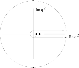
Figure 1: The integration contour in the complex $q^{2}$ plane. The dashed line indicates the part at infinity. Dots denote isolated poles related to stable particles. The thick line is the continuous part of the spectrum.

applied to $T^{FF}(p^{2})/[(p^{2})^{N}(p^{2}-q^{2})]$, $(N\geq 0)$, and often to a circular origin-concentric contour of infinite radius deformed to spare out the positive real axis. Closing the circle at a finite radius $s_{0}<\infty$ leads to so-called finite-energy sum rules [62, 63] which we will not focus on here. We have

$$T^{FF}(Q^{2})=\frac{(-Q^{2})^{N}}{\pi}\int_{0}^{\infty}ds\ \frac{\mbox{Im}\ T^{FF}(s)}{s^{N}(s+Q^{2})}-\frac{\left.d^{N}(T^{FF}(t)\times t)/dt^{N}\right|_{t=0}}{N!}\ (-Q^{2})^{(N-1)}\,,$$ (4)

where $Q^{2}=-q^{2}>0$, $N>0$ and it has been assumed that the integral along the circle vanishes, i.e. for a given $N$ the amplitude $T^{FF}$ has an according behavior at infinity. For $N=0$ the second term on the right-hand side of Eq. (4) is omitted. The quantity $\frac{\left.d^{N}(T^{FF}(t)\times t)/dt^{N}\right|_{t=0}}{N!}$ is called subtraction constant. It is irrelevant if a so-called Borel transformation is applied to the dispersion relation Eq. (4), see below.

The discontinuity of $T^{FF}(q^{2})$ across the cut and the residues of isolated poles are related to the hadronic spectral function $\rho^{FF}(s)$ which follows from an insertion of a complete set of hadron states inbetween the currents of Eq. (1). It is proportional to the total hadronic cross section in the considered channel. This is also known under the name Optical Theorem. For example, the total hadronic cross section $\sigma$ for the process

$$e^{+}e^{-}\to\gamma\to\mbox{hadrons with isospin I=1}$$ (5)

according to the Optical Theorem is related to $\mbox{Im}\ T^{33}$ (associated with the current of Eq. (2)) as [33, 34, 35]

$$\sigma(e^{+}e^{-}\to\gamma\to\mbox{hadrons with isospin I=1})=\frac{16\pi^{2}\alpha_{e}^{2}}{s}\mbox{Im}\ T^{33}(s)\,,$$ (6)

where $\alpha$ denotes the electromagnetic fine-structure constant. In sum rule applications one either substitutes a fit to the low-energy spectrum together with the perturbative QCD spectrum for $s$ greater than the threshold $s_{0}$ for $\mbox{Im}\ T^{FF}(s)\propto\rho^{FF}(s)$ to determine unknown vacuum parameters, see below, or one assumes the dominance of the lowest-lying hadron within the resonance region in a given channel and determines its properties from known vacuum parameters. This leads us to the SVZ approach to the left-hand side of Eq. (4) employing the so-called Operator Product Expansion (OPE) in QCD.

The OPE was originally proposed by K. Wilson [36] in the framework of a so-called skeleton theory for hadrons. The claim is that for a given theory a nonlocal product of composite operators $O_{1}(x)O_{2}(0)$ can usefully be expanded into a series

$$O_{1}(x)O_{2}(0)=\sum_{D,{i_{D}}}c_{D}^{i_{D}}(x)\ O_{D}^{i_{D}}(0)\ .$$ (7)

involving local operators $O_{D}^{i_{D}}(0)$ of increasing mass-dimension $D$ and c-number coefficients $c_{D}^{i_{D}}(x)$ - the so-called Wilson coefficients - as long as the (Euclidean) distance $|x|$ is small compared to the inverse of the highest dynamical mass scale in the theory. The OPE can be shown to exist in perturbation theory, see for example [38]. In Eq. (7) the index $i_{D}$ runs over all possible, independent operators of dimension $D$. Taking the vacuum average of Eq. (7), only scalar contributions survive as a consequence of the Poincaré invariance of this state.

Applying the OPE to a correlator of gauge invariant currents in QCD, the scalar amplitudes in a given current correlator are expanded into a series of the form Eq. (7). The participating operators, such as ${\bf 1}$, $\frac{\alpha}{\pi}G^{a}_{\mu\nu}G^{\mu\nu}_{a}$ and $m(\bar{u}u+\bar{d}d)$, are gauge invariant, and the associated Wilson coefficients are perturbatively expanded in powers of $\alpha_{s}$. By definition, the expectation in the perturbative vacuum of the expansion singles out the unit operator ${\bf 1}$.

In general, Wilson coefficients and operator averages depend on a normalization scale $\mu$ at which the perturbatively calculable short-distance effects contained in the former are separated from the parametrized long-distance behavior induced by nonperturbative fluctuations in the latter. If the currents of interest are conserved then the associated correlator should not depend on any factorization convention. In this case a residual $\mu$ dependence of the OPE is an artefact of the truncation of the $\alpha_{s}$ series in each coefficient function. An improved scale dependence of the Wilson coefficients can be obtained by solving perturbative renormalization group equations. At higher order in $Q^{-1}$ operators mix and anomalous dimension matrices must be diagonalized to decouple the system of evolution equations [21], see also [33]. Vacuum averages of nontrivial QCD operators defined at $\mu$ are universal, that is, channel-independent parameters. They are the QCD condensates. These parameters have to be extracted from experiment, and they induce (up to logarithm’s arising from anomalous operator dimensions) (negative) power corrections in $Q$. Already in the seminal paper [21] it was realized that the OPE in QCD can at best be an asymptotic expansion since small-sized instantons spoil the naive power counting $\left(\frac{\Lambda_{QCD}}{Q}\right)^{D}$ for operators of the form $G^{D/2}$ starting at the critical dimension $D=12$. This estimate was obtained from a dilute gas approximation for the instanton ensemble. Ever since, the discussion about the validity of the OPE in the light of its possible asymptotic nature, nonperturbative, nonlocal effects and the tightly related issue of local quark hadron duality has never faded away (see for example [38, 142, 143, 144, 145, 146, 147, 42, 43]). No definite conclusions have been reached although valuable insights were obtained in model approaches. To shed light on this discussion is in the main purpose of the present review. It is stressed here, however, that the phenomenological success of many QCD sum-rule applications using ’practical’ OPEs, typically truncated at $D=6,8$, supports the pragmatic approach of Shifman, Vainshtein and Zakharov of ‘scratching’ into the nonperturbative regime by ignoring questions of OPE convergence. For example, the prediction of the mass of the $\eta_{c}$ at 3.0 GeV by a sum rule in the pseudoscalar $\bar{c}c$ channel matches almost precisely the result of a later experiment [41].

Let us now discuss how Wilson coefficients are computed in practice. The perturbative part of a mesonic current correlator is the usual vacuum polarization function. In the case of electromagnetic currents this function was calculated to 4-loop accuracy in [133, 132]. For the calculation of the Wilson coefficients appearing in power corrections two methods are known. The so-called background-field method [130] uses a Wick expansion of the time-ordered product of currents and interaction Lagrangians. Quark propagation is considered in a gauge-field background and the Fock-Schwinger or fixed-point gauge $x^{\mu}A_{\mu}(x)=0$ is used. In the background-field method the gauge field and the quark field away from the origin are expressed in powers of adjoint and fundamental covariant derivatives acting on the field strength and the quark field at the origin, respectively. It is tacitly assumed in all practical applications that the gauge invariance of nonlocal operator products, as they arise in the Wick expansion, is ensured by straight Wilson lines

$$W(z_{i})={\cal P}\exp\left[ig\int_{0}^{z_{i}}dy^{\mu}\,A_{\mu}(y)\right]\,,\ \ \ y_{\mu}=\xi z_{\mu}\,,\ \ \ 0\leq\xi\leq 1\,,$$ (8)

which connect a field at $z_{i}$ with a field at the base point zero (see [140] for an exhaustive discussion). The symbol ${\cal P}$ in Eq. (8) denotes the path-ordering prescription. The gauge invariance of the resulting nonlocal operators is at the price of allowing for gauge parallel transport only along straight lines connecting to the base point zero. The method does not consider fluctuating gluons and therefore the computation of radiative corrections in Wilson coefficients is out of reach. It has been applied to the computation of Wilson coefficients for the gluonic operators of the form $g^{3}G^{3}$, $g^{4}G^{4}$, and $g^{2}(DG)^{2}=g^{4}j^{2}$ which induce the relevant power corrections in heavy quark correlators [137, 138, 140]. A second method, which allows for the consideration of radiative corrections, works as follows. Project out a particular Wilson coefficient in an OPE of interest by sandwiching the associated T product of currents with (hypothetical) external quark and/or gluon states, separate off the structure belonging to the corresponding operator, and take the limit of vanishing external momenta. The calculation can be carried out at any order in perturbation theory - radiative corrections can be considered. This method was used in [21] and in [135, 136] together with the background method.

Having discussed the two sides of the dispersion relation (4) we will now review refinement procedures for the practical evaluation of sum rules. Typically, precise information about the spectral function in a given channel is limited to the lowest lying resonance. It can thus be important to apply a weight function to the spectral function which suppresses the high-energy tail to sufficiently reduce the error in the spectral integral. A Borel transformation, which acts on the sum rule (4) by an application of the operator

$${\bf L}\equiv\lim_{{Q^{2}\to\infty,\ N\to\infty}\atop Q^{2}/N\equiv M^{2},\ M^{2}\ \mbox{{\tiny fixed}}}\frac{(-1)^{N}}{(N-1)!}\ (Q^{2})^{N}\left(\frac{\partial}{\partial Q^{2}}\right)^{N}\,,\ \ \ \ \ \ \ \ \ \ \ \ \ \ (Q^{2}=-q^{2})$$ (9)

is designed to do precisely this. On the spectral side it generates an exponential $\sim\exp[-s/M^{2}]$ as opposed to the power suppression $\sim 1/(s+Q^{2})$ at high energy and on the OPE side power corrections in the Borel parameter $M$ are factorially suppressed in the mass-dimension. A physical parameter, which is extracted from the sum rule, should be independent of $M$ within the so-called stability window. This region of values for $M$ is interpreted as the interval where the spectral side of the sum rule indeed approximates the OPE expression. Hadron parameters are extracted in this region.

It sometimes proves useful to suppress the high-energy tail of the spectral function by a higher integer power of $s$ and then look at the insensitivity of the sum rule under variations in this power. In this case one considers various derivatives of the sum rule (4) with respect to the external momentum $Q^{2}$. This leads to a set of moment sum rules.

4 Seminal sum-rule examples

Violations of local quark-hadron duality are believed to have a mild effect on QCD sum rules. We review specific QCD sum rules for (axial)vector mesons in this section. In view of future and ongoing experiments at facilities like the large hadron collider (LHC) and the relativistic heavy ion collider (RHIC), respectively, we also discuss the in-medium approach to QCD sum rules for (axial)vector current-current correlators.

4.1 Borel sum rules for light (axial) vector meson currents

We consider the following currents, which interpolate to the $\rho,\omega$, and $A_{1}$ resonances:

$$j_{\mu}^{\rho,\omega}\equiv\frac{1}{2}(\bar{u}\gamma_{\mu}u\mp\bar{d}\gamma_{\mu}d)\,,\ \ \ j_{\mu}^{A_{1}}\equiv{\cal TP}\frac{1}{2}(\bar{u}\gamma_{\mu}\gamma_{5}u-\bar{d}\gamma_{\mu}\gamma_{5}d)\,.$$ (10)

The operation ${\cal TP}$ projects the axial current onto its conserved part which allows to discard the pion pole contribution in the spectral function of its correlator. After separating off a transverse tensor structure $q_{\mu}q_{\nu}-q^{2}g_{\mu\nu}$ the OPEs for the current-current correlators $T^{\rho,\omega}$, and $T^{A_{1}}$ in vacuum are given as[79]:

$$T^{\rho,\omega} = -\frac{1}{8\pi^{2}}\left(1+\frac{\alpha_{s}(\mu^{2})}{\pi}\right)\log\left(\frac{Q^{2}}{\mu^{2}}\right)+\frac{m_{q}}{2Q^{4}}\left\langle\bar{u}u+\bar{d}d\right\rangle+\frac{1}{24Q^{2}}\left\langle\frac{\alpha_{s}}{\pi}G^{a}_{\mu\nu}G^{a}_{\mu\nu}\right\rangle-$$

$$\frac{\pi\alpha_{s}}{2Q^{6}}\left\langle\left(\bar{u}\gamma_{\mu}\gamma_{5}\lambda^{a}u\mp\bar{d}\gamma_{\mu}\gamma_{5}\lambda^{a}d\right)^{2}\right\rangle(\mu)-\frac{\pi\alpha_{s}}{9Q^{6}}\left\langle\left(\bar{u}\gamma_{\mu}\lambda^{a}u+\bar{d}\gamma_{\mu}\lambda^{a}d\right)\sum_{q=u,d,s}\bar{q}\gamma_{\mu}\lambda^{a}q\right\rangle(\mu)\,,$$

$$T^{A_{1}} = -\frac{1}{8\pi^{2}}\left(1+\frac{\alpha_{s}(\mu^{2})}{\pi}\right)\log\left(\frac{Q^{2}}{\mu^{2}}\right)-\frac{m_{q}}{2Q^{4}}\left\langle\bar{u}u+\bar{d}d\right\rangle+\frac{1}{24Q^{2}}\left\langle\frac{\alpha_{s}}{\pi}G^{a}_{\mu\nu}G^{a}_{\mu\nu}\right\rangle-$$ (11)

$$\frac{\pi\alpha_{s}}{2Q^{6}}\left\langle\left(\bar{u}\gamma_{\mu}\lambda^{a}u-\bar{d}\gamma_{\mu}\lambda^{a}d\right)^{2}\right\rangle(\mu)-\frac{\pi\alpha_{s}}{9Q^{6}}\left\langle\left(\bar{u}\gamma_{\mu}\lambda^{a}u+\bar{d}\gamma_{\mu}\lambda^{a}d\right)\sum_{q=u,d,s}\bar{q}\gamma_{\mu}\lambda^{a}q\right\rangle(\mu)\,,$$

where a one-loop correction is included in the perturbative part, the Wilson coefficients in the power corrections are given without radiative corrections, $\mu$ denotes the normalization point, degenerate light-quark masses $m_{q}=m_{u}=m_{d}$ have been assumed, and $\lambda^{a}$ are SU(3) generators in the fundamental representation normalized to tr$\lambda^{a}\lambda^{b}=2\delta^{ab}$. In contrast to dimension four the operator averages at $D=6$ depend on the normalization point $\mu$ logarithmically [21]. For simplicity and because effective anomalous operator dimensions are small, we neglect this dependence here.

On the spectral side, we use a zero-width model for the lowest resonance and approximate higher resonances by a (channel-dependent) perturbative continuum starting at threshold $s^{mes}_{0}$ (see for example [34]). The resonance part involves a meson-to-vacuum element. In the case of vector mesons it is parametrized as

$$\left\langle 0|j_{\mu}^{mes}|mes(p)\right\rangle\equiv f_{mes}m_{mes}\epsilon_{\mu}\,$$ (12)

where $f_{mes}$ $(mes=\rho,\omega)$ is a decay constant and $\epsilon_{\mu}$ the meson’s polarization vector. The contributions of the pion continuum to the spectral functions for $s\leq s_{0}$ are for practical reasons neglected here. In Fig. 2 the experimental data for the sum of $\rho$ and $A_{1}$ spectral functions is shown for center-of-mass energies up to $\sqrt{s}=\sqrt{3}$ GeV. The two resonance peaks at $m^{2}_{\rho}\sim(0.77)^{2}\,\mbox{GeV}^{2}=0.59\,\mbox{GeV}^{2}$ and $m^{2}_{A_{1}}\sim(1.26\,\mbox{GeV})^{2}=1.59\,\mbox{GeV}^{2}$ are clearly visible. A similar situation holds in the $\omega$ channel. After Borel transformation we obtain the following sum rules

Figure 2: The sum of $\rho$ and $A_{1}$ spectral functions as measured by the Aleph collaboration in $\tau$ decays. Plot taken from [179].

$$T^{\rho,\omega,A_{1}}(M^{2})=\frac{1}{M^{2}}\left[f_{mes}^{2}\mbox{e}^{-m_{mes}^{2}/M^{2}}+\frac{1}{8\pi^{2}}(1+\frac{\alpha_{s}}{\pi})\mbox{e}^{-s_{0}/M^{2}}\right]\,,\\$$

where the left-hand side of Eq. (4.1) can is represented by the Borel transforms of the respective OPEs (applying the operator (9) term by term). To extract information on the meson parameters one solves the sum rule, Eq. (4.1), for the resonance piece $R\equiv f_{mes}^{2}\mbox{e}^{-m_{mes}^{2}/M^{2}}$. Assuming the coupling constants $f_{mes}$ and the resonance masses $m_{mes}$ to be sufficiently insensitive to changes in the Borel parameter $\tau\equiv\frac{1}{M^{2}}$, one can solve for $m_{mes}$ by performing a logarithmic derivative

$$m_{mes}^{2}=-\frac{\partial}{\partial\tau}\mbox{log}\ R\,.$$ (13)

Using the following numerical values for the condensates

$$\left\langle\bar{q}{q}\right\rangle\ (\mu=1\ \mbox{GeV}) = -(250\ \mbox{MeV})^{3}\,,$$

$$\ \left\langle\frac{\alpha}{\pi}G^{a}_{\mu\nu}G_{a}^{\mu\nu}\right\rangle\ (\mu=1\ \mbox{GeV}) = 0.012\ \mbox{GeV}^{4}\,,$$ (14)

a continuum threshold $s_{0}^{\rho}=1.5\,\mbox{GeV}^{2}$, and approximating the four-quark condensate by squares of chiral condensate by assuming exact vacuum saturation [21] (taking place in the limit of a large number of colors, $N_{c}\to\infty$), one obtains a dependence of $m_{\rho}$ on $\tau$ as shown in Fig. 3. We have neglected the contribution of the quark condensate at D=4 since it is numerically small compared to the gluon-condensate $m_{q}/\Lambda_{QCD}\ll 1$.

Figure 3: The dependence of $m_{\rho}$ on the Borel parameter $\tau$.

Fig. 3 clearly indicates that the sum rule for the $\rho$ meson is stable in the Borel mass for values around $M^{2}=0.8\,\mbox{GeV}^{2}$. One obtains qualitatively similar results in the $\omega$ and $A_{1}$ channels [22].

4.2 Quarkonia moment sum rules

So far we have considered light-quark channels using Borel transformed sum rules. In the case of mesons containing a heavy-quark pair moment sum rules turn out to be useful [64]. The methods of Ref. [64] have been developed further over the years and often applied to determine the mass of the bottom quark (for a review see [65]). To be sensitive to the value of the quark mass the focus in the past was mainly on large moments since these suppress the perturbative continuum [22, 139, 140]. In general, moment sum rules require a precise analysis of the quarkonium threshold and an according definition of the quark mass [70]. We briefly introduce the method here since we will rely on it in Sec. 7.3.2.

One starts with the correlator (1) where now light-quark currents of definite SU(3)_F quantum numbers are replaced by heavy-quark currents such as $j_{\mu}^{h}=\bar{h}\gamma_{\mu}h$, $h$ denoting one of the heavy-quark fields $c,b,t$. Since this current is conserved we may again separate off a transverse structure $(q_{\mu}q_{\nu}-q^{2}g_{\mu\nu})$ and then only consider the scalar amplitude $T^{\bar{h}h}$. In contrast to the light-quark case, where the OPE essentially is an expansion in $\frac{\Lambda_{QCD}}{Q}$, the scale that power-suppresses nonperturbative corrections is naturally given by the heavy-quark mass $m_{h}$. One therefore expands both sides of the sum rule in powers of the dimensionless parameter $z\equiv Q^{2}/(4m_{h}^{2})$,

$$T^{\bar{h}h}(Q^{2})=\frac{3Q_{c}^{2}}{16\pi^{2}}\sum_{n\geq 0}C_{n}z^{n}\,,$$ (15)

where $Q_{c}$ denotes the electric charge of the heavy quark, and compares coefficients $C_{n}$. These can be expressed in terms of the moments ${\cal M}_{n}$, defined as

$${\cal M}_{n}=\left.\frac{1}{n!}\left(-\frac{d}{dQ^{2}}\right)^{n}T^{\bar{h}h}(Q^{2})\right|_{Q^{2}=0}\,,$$ (16)

as follows

$${\cal M}_{n}=\frac{Q_{c}^{2}}{16\pi^{2}}\left(\frac{-1}{4m_{h}^{2}}\right)^{n}C_{n}\,.$$ (17)

The perturbative part of the coefficient $C_{n}$ is known up to order $\alpha_{s}^{2}$ and $n=8$ [256, 67, 68]. It can be written as

$$C_{n}=C_{n}^{(0)}+\frac{\alpha_{s}(\mu)}{\pi}\left(C_{n}^{(10)}+C_{n}^{(11)}l_{m_{h}}\right)+\left(\frac{\alpha_{s}(\mu)}{\pi}\right)^{2}\left(C_{n}^{(20)}+C_{n}^{(21)}l_{m_{h}}+C_{n}^{(22)}l^{2}_{m_{h}}\right)\,,$$ (18)

where $l_{m_{h}}$ is a short-hand for $\log(m_{h}^{2}/\mu^{2})$ and the coefficients $C_{n}^{(\cdots)}$ are listed up to $n=8$ in [69]. The nonperturbative part of the moment ${\cal M}_{n}$, induced by the condensates $\left\langle g^{2}G^{a}_{\mu\nu}G^{a}_{\mu\nu}\right\rangle,\left\langle g^{3}f^{abc}G^{a}_{\mu\nu}G^{b}_{\nu\lambda}G^{c}_{\lambda\mu}\right\rangle$, and $\left\langle g^{4}j_{\mu}^{a}j_{\mu}^{a}\right\rangle$, $j_{\mu}$ being the light-flavor singlet current, was calculated in [138, 140] by using the background-field method. In our convention, Eq. (16), the corresponding expressions are listed in [73]. Low-$n$ moments are more sensitive to the spectral continuum, $large$-n moments to the resonance part of the spectrum. The former probe the relativistic part of the spectrum, and an expansion in $\alpha_{s}$ is appropriate. The latter probe the nonrelativistic physics in the quarkonium threshold region. The expansion parameter $\alpha_{s}$ is modified by the velocity of the heavy quark and given as $\sqrt{n}\alpha_{s}$. For, say, $n>4$ a resummation of the spectrum to all orders in $\sqrt{n}\alpha_{s}$ by a Schroedinger equation for the bound state should be performed (for a review see [71]).

On the phenomenological side the correlator is expressed in terms of a dispersion integral. In terms of the heavy-quark pair cross section $\sigma_{e^{+}e^{-}\to c\bar{c}+X}$ and muon pair cross section $\sigma_{e^{+}e^{-}\to\mu^{+}\mu^{-}}$ in $e^{+}e^{-}$ annihilations this leads to the following expression for the moments

$${\cal M}^{exp}_{n}\,=\,\frac{1}{12\pi^{2}\,Q_{c}^{2}}\,\int\frac{ds}{s^{n+1}}\,\frac{\sigma_{e^{+}e^{-}\to h\bar{h}+X}(s)}{\sigma_{e^{+}e^{-}\to\mu^{+}\mu^{-}}(s)}\,.$$ (19)

It is obvious from Eq. (19) that with increasing $n$ the hadron spectrum is probed at lower and lower center-of-mass energy $\sqrt{s}$. To reliably extract the quark-mass parameter $m_{h}$ at high $n$ therefore needs a high-precision treatment of the spectral function close to the threshold of quarkonium production. When $m_{c}$ was first estimated on parton level only the lowest four moments were considered[22].

If instead of analyzing the parameter $m_{h}$ by using low moments one wants to estimate power corrections it is better to consider the ratio $r_{n}\equiv\frac{{\cal M}_{n}}{{\cal M}_{n-1}}$ of adjacent moments since, contrary to the moments themselves, this quantity does not contain high powers of $m_{h}$ for large $n$. Large $n$ are needed to be sensitive to the nonperturbative information of the resonance region. The ratio-of-moment analysis thus is less sensitive to the error in the extraction of $m_{h}$ and therefore more reliable. Historically, the value of the gluon condensate $\left\langle\frac{\alpha_{s}}{\pi}G^{a}_{\mu\nu}G^{a}_{\mu\nu}\right\rangle\sim 0.012\,\mbox{GeV}^{4}$ was first estimated using a stability analysis of $r_{n}$ for $n=2\cdots 10$ in the J/$\psi$ channel including resonances up to $\psi(4400)$ and the usual perturbative continuum model with threshold $s_{0}=(4.2\,\mbox{GeV})^{2}$. In Sec. 7.3.5 we will have to go beyond the dimension four power correction when we analyze the ‘running’ of the gluon condensate in the framework of a reshuffled OPE containing nonlocal nonperturbative information.

4.3 QCD sum rules in the (axial)vector meson channel at $T,\mu_{B}>0$

In this section we address the case of a QCD current correlator in the (axial)vector-meson channel and its OPE inside a hot or dense medium. On the one hand, the high-temperature situation is of relevance since the properties of mesonic resonances (width and peak positions) in such an environment are measured in ongoing and future experiments at RHIC and LHC, respectively. To do this, the measurement of the, almost unperturbed by the nuclear environment, invariant mass spectrum of dileptons is carried out. Dileptons, produced in the early stages of a relativistic heavy-ion collision by vector meson decay, tell us about the mass and the width of the primary. A sudden ‘melting’ of the spectrum should unambiguously indentify the deconfinement transition. QCD sum rules are predestined to make predictions of the $T$ dependence of spectral parameters [74, 76, 78, 79, 81, 84, 87, 88, 89, 90, 91]. On the other hand, there are interesting effects inside a cold baryon-rich nuclear medium which can be probed by heavy ion colliders operating at lower center-of-mass energy. For example, isospin resonance mixing can be induced by an isospin-asymmetric environment. This is possibly accessible to a theoretical treatment using QCD sum rules and assuming the nuclear environment to be modelled by a dilute gas of nucleons [96, 97, 99, 100, 103, 104, 105, 106, 107, 108, 109, 111, 112, 113].

The main focus of our brief review of the (axial)vector-meson sum rules in medium is on the occurrence of a twist expansion when replacing the vacuum average over a bilocal current product by a Gibbs average

$$\left\langle 0|\cdots|0\right\rangle\to\left\langle\left\langle\cdots\right\rangle\right\rangle\equiv Z^{-1}\mbox{Tr}\mbox{e}^{-\beta(H-\mu_{B}Q_{B})}\cdots\,,$$ (20)

where $Z\equiv\mbox{Tr}\mbox{e}^{-\beta(H-\mu_{B}Q_{B})}$ denotes the grand-canonical partition function for the QCD Hamiltonian $H$, $\mu_{B}$ defines a baryon chemical potential, and $Q_{B}\equiv\int d^{3}x\,j_{0}^{B}$ is the associated, conserved baryon charge. A resummation of such an expansion genuinely takes nonperturbative nonlocalities in the associated hadron states into account. At finite temperature $T$ a small expansion parameter $T/Q$ exists ($T<\Lambda_{QCD},Q\sim 1\,\mbox{GeV}$), and such a resummation is apparently not needed. The situation is quite different at finite nucleon density, where the expansion parameter is $m_{p}/Q$ ($m_{p}$ the proton mass) and a (partial) resummation of the twist expansion is imperative. The present section serves as a prerequiste to Sec. 7, where it is pointed out that the consideration of nonperturbative nonlocalities in vacuum OPEs is necessary for a good description of certain hadron properties.

4.4 Light (axial)vector mesons at $T>0$

The pioneering work in formulating QCD sum rules for the case of finite temperature and/or baryon density was launched by A. I. Bochkarev and M. E. Shaposhnikov in 1985 [74]. In particular, the $\rho$-meson channel at finite temperature, as it was first treated in this paper, has been revisited several times over the years [75, 76, 77, 81, 82, 80, 79, 83, 87, 88, 84, 91, 89, 90, 106] because a number of substantial points were overlooked in [74] on both sides of the sum rule.

Let us first discuss the basic points of the approach in [74] and its application to the $\rho^{0}$ channel. Instead of using a causal $T$ product the formulation relies on a the retarded ordering of currents because of its more adequate analytical properties. In either case, the correlator of conserved currents $T_{\mu\nu}$ can be decomposed into two invariants $T_{1}(q_{0}^{2}=(u_{\mu}q^{\mu})^{2},q^{2})$ and $T_{2}(q_{0}^{2}=(u_{\mu}q^{\mu})^{2},q^{2})$ since through the presence of a preferred rest frame a new covariant $u_{\mu}$=(1,0,0,0) - the four-velocity of the heat bath - exists besides the external momentum $q_{\mu}$, and therefore

$$T_{\mu\nu}(q,u)=(q_{\mu}q_{\nu}-q^{2}\,g_{\mu\nu})T_{1}+(u_{\mu}-\omega\frac{q_{\mu}}{q^{2}})(u_{\nu}-\omega\frac{q_{\nu}}{q^{2}})T_{2}\,,$$ (21)

where $\omega=u^{\mu}q_{\mu}$. In the limit $\vec{q}\to 0$, however, $T_{1}$ and $T_{2}$ depend on each other, and it suffices to consider only one of them. By truncating the trace in the Gibbs average (20) to the vacuum and one-particle pion states (1-$\pi$ states) (dilute pion-gas approximation), for $T\leq 160\,$MeV this is well justified due to the chiral gap in the spectrum ($m_{\pi}\sim 140\,$MeV, $m_{\rho}\sim 770\,$MeV), a Borel sum rule for the $\rho^{0}$ channel at finite temperature was derived in [74] in the limit $\vec{q}\to 0$. Evaluating the spectral side in this approximation, there appears a zero-temperature 2-$\pi$ continuum weighted by a function $\tanh(\sqrt{s}/4T)$, usually neglected in vacuum sum rules, and, in addition, a scattering contribution to the spectral density,

$$\propto\delta(s)\theta(\omega^{2}-4m_{\pi}^{2})n_{B}(\omega/2T)\,,$$ (22)

accounting for a 1-$\pi$ intermediate state scattering off the current into a heat-bath pion and vice versa [76]. The $\rho$-meson contribution to the spectral function is as in vacuum since the 1-$\pi$-to-$\rho$ matrix element of the current vanishes in the Gibbs-trace. At $s>s_{0}$ the spectrum is approximated by thermal QCD perturbation theory. There is a quark-antiquark continuum and a scattering term. The latter arises from the interaction of the current with quarks in the heat bath. At $T\sim 130\,$MeV it amounts to about three times the corresponding pion contribution. This shows the relative suppression of the pion scattering term in the hadronic part of the spectrum.

On the OPE side, the $T$ dependence of the dimension-six (four-quark) operators in Eq. (4.1) that contribute to the vacuum correlator was treated in [74] by applying the fluctuation-dissipation theorem, that is, by expressing the Gibbs averages of local operators through spectral functions in the respective channels

$$\left\langle\left\langle A(0)B(0)\right\rangle\right\rangle=\pi\int\frac{d^{4}p}{(2\pi)^{4}}\coth(\omega/2T)\rho(\omega,\vec{p},T)\,,$$ (23)

where $\rho$ is the absorptive part of the retarded correlator of the two currents $A$ and $B$. In order to make sense of such a spectral function the original current product has to be Fierz rearranged into products of gauge invariant currents. Each of these products can then be evaluated using (23). For alternative ways of calculating pion averages over four-quark operators see below [79] and [119]. For dimension-four operators this does not apply and some not too solid arguments were used to conclude that the $T$ dependent part of their Gibbs averages is small [74] and therefore can be neglected. As a result of their Borel analysis Bochkarev and Shaposhnikov find that the both the $\rho$ mass parameter and the spectral continuum threshold $s_{0}$ experience a drastic drop at $T\sim 150\,$MeV.

Three comments are in order: (i) On the spectral side in [74] the fact was not taken into account that at finite $T$ the axial and the vector channel mix, and consequently that both resonances $\rho$ and $A_{1}$ should appear in the spectral function of the $\rho^{0}$ channel. In the dilute pion-gas approximation of [74] this was first shown in [76] up to first order in the parameter $\epsilon\equiv\frac{T^{2}}{6f_{\pi}^{2}}$. Powers of $\epsilon$ arise by reducing 1-$\pi$, 2-$\pi$, 3-$\pi$, $\cdots$ states arising in the Gibbs-trace (20) by means of the LSZ reduction formula, neglecting their momenta, and using PCAC and current algebra in the chiral limit. Taking into account only these finite-$T$ corrections, the correlators $T^{\rho,A_{1}}_{\mu\nu}(q,T)$ are expressible as a superposition of vector and axial-vector correlators $T^{\rho,A_{1}}_{\mu\nu}(q,0)$ at zero temperature. Up to order $T^{2}$ only the $\epsilon$ expansion contributes, and one obtains,

$$T^{\rho}_{\mu\nu}(q,T) = (1-\epsilon)T^{\rho}_{\mu\nu}(q,0)+\epsilon T^{A_{1}}_{\mu\nu}(q,0)\,,$$

$$T^{A_{1}}_{\mu\nu}(q,T) = (1-\epsilon)T^{A_{1}}_{\mu\nu}(q,0)+\epsilon T^{\rho}_{\mu\nu}(q,0)\,.$$ (24)

Thus the resonance poles of the $\rho$ and $A_{1}$ mesons do not move as a function of $T$ (and would not to any order in $\epsilon$ if this was the only expansion for $T$ corrections). The relative weight of the $A_{1}$ meson in the spectral integral, however, increases with growing temperature. Interestingly, it was found in [76] by a Borel sum-rule analysis applied to a single-resonance spectral function (erroneously, since the $\rho$ mass does not shift at order $\epsilon$) that the $\rho$ mass shifts towards higher values as $T$ grows. One still can interprete this result in terms of the spectral weight moving towards higher invariant mass-squared $s$ as $T$ increases (growing importance of the $A_{1}$ resonance, see Eq. (4.4)). Except for [84] none of the QCD sum rule analysis subsequently performed, which all assumes a single resonance in the spectrum of the (axial)vector channel, has reproduced this behavior. Going to order $T^{4}$, there is an order $\epsilon^{2}$ correction, arising from the zero-momentum 2-$\pi$ states, but also a correction of order $\left(T^{2}/Q^{2}\right)^{2}$ which originates from finite pion momenta in the 1-$\pi$ state. The latter was estimated in [83] by expressing the two invariants $T^{\pi}_{1,2}$, defined in analogy to Eq. (21) with $u_{\mu}\to p_{\mu}$ and $\omega\to\nu=p^{\mu}q_{\mu}$ in the 1-$\pi$ matrix element of the current product, in terms of the measured pion structure functions $F_{1,2}(x,q^{2})$, $x=Q^{2}/2\nu$, using dispersion relations. There is a $\left(T^{2}/Q^{2}\right)^{2}$ correction in both the Lorentz invariant and violating parts $T_{1,2}$, respectively. These terms are induced by nonscalar condensates in the OPE leading us to the next comment on [74].

(ii) In [74] only scalar operators were considered in the OPE. The O(4)-invariance is, however, reduced to an O(3)- or rotational invariance by the presence of the heat bath, and thus a number of additional operators are allowed to contribute to the OPE. This was first noticed in [79] where a systematic twist-expansion was used to identify the relevant, nonscalar operators. The gluonic stress, contributing at dimension four, was further investigated in [82] and in [87, 88] in view of operator mixing under a change of the renormalization scale. In [79] the 1-$\pi$ matrix elements of operators, such as parts of $\theta_{00}$ at dimension four ($\theta_{\mu\nu}$ denotes the QCD energy-momentum tensor) and operators of the type $\bar{q}\gamma_{0}D^{3}_{0}q$ at $D=6$, with non-zero twist - all other operator averages were omitted because of non-calculability - were evaluated using pionic parton distribution functions in the leading-order scheme and the parametrization of [92] at the sum rule scale $\mu=1\,$GeV. As noticed above on general grounds, the thermal phase-space integrals over 1-$\pi$ matrix elements of pure-quark scalar operators in the OPE are expressible in terms of zero-temperature condensates and expanded in powers of $\epsilon$ only by applying the LSZ reduction formula, PCAC, and current algebra [79]. The 1-$\pi$ matrix elements of the operator $\alpha_{s}/\pi\,G^{2}$ can be calculated by using the QCD trace-anomaly [95], $\theta^{\mu}_{\mu}=-1/8\pi(11-2/3N_{F})\alpha_{s}G^{2}+\sum_{q}m_{q}\bar{q}q$. As a result, the matrix element is proportional to the pion mass and thus vanishes in the chiral limit. Even for realistic pion masses the $T$-induced shift of the gluon condensate is negligible [79]. Assuming a single, narrow resonance plus scattering term plus continuum model for the spectral side, the Borel analysis of [79] indicates a drastic decrease of the $\rho$ mass and the continuum threshold $s_{0}$ at $T\sim 160-170\,$MeV. Notice that with the choice $\sqrt{s_{0}(T=0)}\sim 1.3\,$GeV$>m_{A_{1}}(T=0)=1.26\,$GeV in [79] the $A_{1}$ resonance can effectively be viewed as a part of the perturbative continuum. A mixing of the $A_{1}$ and $\rho$ channels was noticed in [79] on the OPE side, in accord with the general result in [76]. Similar results were obtained for the $\omega$ and $A_{1}$ channels.

(iii) No attempt was made in [74] to consider a $T$ dependence of the vacuum state itself. This is suggestive since parameters like $f_{\pi}$, entering the average over the pion state in Eq. (20), have a $T$ dependence which, in the case of $f_{\pi}$, is calculable in thermal chiral perturbation theory [78]. Chiral perturbation theory also predicts the $T$ dependence of the quark condensate [93]. For an investigation of the Gell-Mann-Oakes-Renner relation at finite temperature and the calculation of the $T$ dependence of the pion mass relying on finite-energy sum rules see [85]. Nothing, however, is known about the $T$ dependence of parton distribution functions. Assuming that a $T$ dependence of the vacuum state is the dominating dependence of the matrix elements in the Gibbs average (and thus that the $T$ dependence of 1-$\pi$ matrix elements can be neglected - the effect would anyway be of higher order in $T$) and assuming that such a dependence arises only implicitly through a $T$ dependence of the continuum threshold $s_{0}$ (related to a $T$ dependence of the QCD scale $\Lambda_{QCD}$), a scaling of the vacuum averages of operators with powers of their mass dimension $2n$, $(s_{0}(T)/s_{0}(0))^{n}$, was introduced in [84]. A $T$ dependence of the vacuum state is, indeed, suggested by the condensation of center vortices in the confining phase of QCD. These topological objects can be viewed as coherent thermal states themselves, hence the (mild) $T$ dependence of the ground state. Condensed center vortices are apparently responsible for quark confinement and chiral symmetry breaking [86]. The scaling with powers in $s_{0}(T)/s_{0}(0)$ introduced in [84] is an effective, phenomenological way of considering this effect. Note that this scaling does not capture the small effects of omitted, higher hadronic resonances in the Gibbs average. As a result, a positive “mass shift” similar to the one in [76] and, as a byproduct, a moderate drop of the gluon condensate around $T=160\,$MeV, which at least qualitatively is in accord with lattice results [94], was obtained, compare Figs. 4 and 5. Notice that this decrease of about $30$% (for $s_{0}(T=0)=1.5\,$GeV²) as compared to the value at $T=0$ is practically entirely due to the vacuum average and not due to 1-$\pi$ matrix elements.

(iv) The usefulness of thermal, i.e. on-shell quarks (the scattering term), in [74] is quite questionable at low temperatures.

We have seen that thermal, practical OPEs of current-current correlators allow for additional, O(3)-invariant, operators to appear. These operators arise in the Gibbs average from matrix elements over 1-$\pi$ states with nonvanishing spatial momentum. An expansion in powers of $T^{2}/Q^{2}$ arises in the chiral limit. Temperature induced corrections in Gibbs averages over scalar operators can be organized as expansions in two parameters, $T^{2}/6f_{\pi}^{2}$ and $T^{2}/Q^{2}$ (in the chiral limit). The former arises from the (repeated) use of the LSZ reduction formula, PCAC and current algebra treating the pion as a noninteracting, elementary particle in the soft limit; the latter arises from the structure of finite-momentum pions. Since practical vacuum OPEs are, roughly speaking, expansions in $\Lambda_{QCD}^{2}/Q^{2}$ we conclude that the “convergence” of the expansion is not threatened by finite-temperature effects.

Figure 4: The ratio of the $T$ dependent to the vacuum gluon condensate as obtained in [84]. The dot-dashed, solid, and long-dashed curves correspond to continuum thresholds $s_{0}(0)=1.2\,$GeV², $s_{0}(0)=1.5\,$GeV², and $s_{0}(0)=1.8\,$GeV², respectively. The dotted curve shows the effect of perturbative renormalization-group evolution on the vacuum part of four-quark operators when allowing for an effective normalization scale $\sqrt{s_{0}(T)/s_{0}(0)}Q$. Taken from [84].

Figure 5: The $T$ dependence of the gluon condensate as obtained on the lattice. Open circles and squares denote the result obtained for QCD with light and heavy dynamical quarks. The dashed line shows the ideal-gas situation (a formula derived from a scaling argument in [94]), and the solid line is a fit to the lattice result for the $T$ dependence of the gluon condensate. Both lines refer to SU(3) Yang-Mills theory. Taken from [94].

4.5 Vector mesons in nuclear matter

The treatment of current correlation involving (axial)vector mesons in a cold and dense environment using QCD sum rules is technically analogous to the case of finite temperature. Much work has been devoted to the calculation of the change of the mass and width of light vector mesons in a baryon-rich environment [96, 97, 99, 100, 101, 102, 103, 104, 105, 106, 107] (for summaries see [108, 109, 111]) since these should be measurable in terms of the invariant-mass spectra of dileptons emitted in the course of a heavy-ion collision, for an analysis within the Walecka model see [112], at a facility like SIS18 (GSI) with the HADES detector. For an adaption of vector-axialvector mixing to the situation of pions in a nuclear environment see [110]. A sum-rule analysis of the $\rho$-$\omega$ mixing induced by an isospin asymmetric nucleon density $\rho_{N}=\rho_{p}+\rho_{n}$ was performed in [113]. [98], respectively. This effect occurs in vacuum due to the breaking of the SU(2)${}_{\tiny\mbox{F}}$ symmetry by the different electric charges and masses of up- and down-quarks [114]. For a sum-rule analysis of the off-shell situation see [98]. It was shown in [113] that by an appropriate and realistic choice of the isospin asymmetry $\alpha_{np}$ of the nucleonic environment, defined as $\alpha_{np}\equiv\frac{\rho_{p}-\rho_{n}}{\rho_{p}+\rho_{n}}$, the vacuum mixing can either be compensated or enhanced. Most of the above-mentioned works are technically rather involved. A simple and beautiful discussion of the $\rho$ meson (positive) mass shift in nuclei is, however, given in [120]. New developments concerning the treatment of nucleon matrix elements,in particular the ones of four-quark operators, deserve a review article in their own right, for a recent publication relying on the perturbative chiral quark model see [118]. Here we focus on interesting OPE aspects at finite density which hint on a fundamental manifestation of strong interactions at purely Euclidean external momenta in both vacuum and hadron properties: the occurrence of strong nonperturbative correlations characterized by mass scales considerably larger than the perturbative scale $\Lambda_{QCD}$. Let us now briefly review some technical aspects of finite density sum rules.

On the spectral side, a linear-density or dilute-gas approximation for the Gibbs average in (20), which consists of taking into account only the 1-nucleon state besides the vacuum, again leads to the occurrence of a scattering term in the spectral function which is due to the scattering of a bath-nucleon off the current into an intermediate-state nucleon and vice versa. The question whether a treatment of in-medium resonance physics relying on the linear-density approximation is reliable for nucleon densities larger than the saturation density is open. Moreover, the consideration of finite vector-meson width in a pure sum-rule treatment of the resonance seems to be problematic [103]. The sum rule apparently contains too few information to predict both the density dependence of the resonance mass and the width. On the other hand, consistency of a spectral function calculated in the framework of an effective chiral theory with the in-medium OPE of the correlator of the associated currents was obtained in [101].

On the OPE side, O(3)-invariant operators contribute and can be organized in a twist expansion. Their nucleon averages are expressed in terms of integrals over nucleonic quark parton distributions, and a new expansion parameter, $\frac{m^{2}_{p}}{Q^{2}}$, emerges. In practice, one omits twist-four and also mixed operators due to the very limited information about their nucleon averages. The nucleon average over $\bar{q}q$ and $\frac{\alpha}{\pi}G^{2}$ are determined by the nucleon $\sigma$ term and by using the QCD trace anomaly, respectively, see [108]. The treatment of nucleon averages over scalar four-quark operators is not as straight-forward as in the pionic case where chiral symmetry fixes these matrix elements in terms of vacuum averages. One way of proceeding is a mean-field like approximation (MFA) adjusted to the linear-density treatment [96, 100]. For a treatment beyond the linear-density approximation methods have been worked out in [108, 111]. The status of the MFA is quite obscure (for a recent discussion see [106, 107] where the strong sensitivity of the in-medium mass-shifts of $\rho$ and $\omega$ mesons on the value of the in-medium four-quark condensates is stressed).

The evaluation of the Borel sum rules in the $\rho$ channel yields a decrease of the $\rho$ mass [96, 97, 99, 100] with increasing density. As for a the behavior of width and mass no definite conclusion is possible [104, 105]. The old results for the $\omega$ channel in [96, 100, 99], where in comparison to the $\rho$ channel an enhancement of the screening term by a factor of 9 was overlooked [101, 113] and a negative shift of the resonance mass was obtained, are in clear contradiction to more recent analysis [113, 107] which points towards a positive mass shift. Note, however, that the calculation of the $\omega$ mass shift in [101], which is based on a chiral, effective theory, also indicates a negative sign. Consistency with the OPE in this case was reached by applying nuclear ground-state saturation in the same way as in the vacuum:

$$\left\langle\Omega(\rho)|(\bar{q}\gamma_{\mu}\gamma_{5}\lambda^{a}q)^{2}|\Omega\right\rangle=-\left\langle\Omega(\rho)|(\bar{q}\gamma_{\mu}\lambda^{a}q)^{2}|\Omega\right\rangle=\frac{16}{9}\kappa(\rho)\left\langle\Omega(\rho)|\bar{q}q)|\Omega\right\rangle^{2}\,.$$ (25)

This approximation is different from the MFA. In Eq. (25) a density dependence of the correction factor $\kappa$ is allowed for.

Let us make some summarizing comments on practical OPEs at finite nucleon density. (i) As we have seen, a new expansion parameter, $\frac{m^{2}_{p}}{Q^{2}}$, arises in the Gibbs averages over finite-twist, nonscalar operators. Recalling that $m_{p}\sim 940\,$MeV and that the external momentum $Q$ (or the Borel parameter $M$) should be not much larger than $\sim\,$1 GeV to be sensitive to resonance physics and associated power corrections in the OPE, we must conclude that a naive expansion is hardly controlled. However, as it was shown in [115], a summation of the twist-two correction to all orders in $\frac{m^{2}_{p}}{Q^{2}}$ appears to resolve this problem. Such a successful, partial summation of powers of $\frac{m^{2}_{p}}{Q^{2}}$ stresses the need to take nonperturbative nonlocalities in nucleon matrix elements into account. That this is not only true for the nucleon or, more generally, for any sufficiently stable hadron will be shown in detail in Sec. 7 where nonlocalities in vacuum matrix elements are imperative for a good description of certain hadronic properties. A very thorough discussion of the limitations of a local expansion of current correlators in the framework of nucleonic sum rules at isospin-symmetric finite baryonic density and of possible ways of improvement is performed in [116]. This discussion rests on the pioneering work [117] on QCD sum rules for the nucleon at finite baryonic density. (ii) The screening term can dominate the density dependent part of the sum rule (for example in the $\omega$ channel or for the mixed $\rho$-$\omega$ correlator with mean-field treatment of four-quark operator averages) [113]. We can take this as a general indication that most of the density dependence of the resonance parameters is induced by the hadronic model for the rest of the spectral function and not by QCD parameters. So the situation is reversed as compared to vacuum sum-rules, where information on the lowest resonance is obtained in terms of QCD parameters and not in terms of extra hadronic information. (iii) The status of the mean-field treatment of nucleonic matrix over four-quark operators [96, 100] is unclear. It was shown in [107] how a change by a factor of four in the contribution of four-quark operators can already change the sign of the mass-shift of the $\omega$ resonance at nuclear saturation density.

5 OPE and Renormalons

In renormalized perturbation theory the divergent large-order behavior in correlators like the one in (1) can be related to power corrections of these objects [53, 54, 55, 56, 57, 58, 59]. In this section we very briefly discuss the origin of this phenomenon and applications in QCD. We strongly draw upon the review by Beneke [50] which contains the relevant references up to the year 1999. We will explicitly refer to only some of the subsequent developments in applications of renormalons.

In a power-in-$\alpha_{s}$ perturbative expansion up to order $N$ of, say, a two-point current correlator

$$T(\alpha_{s})=\sum_{n=0}r_{n}\alpha_{s}^{n+1}$$ (26)

certain classes of diagrams, which we assume to dominate the expansion in $\alpha_{s}$ in QCD, are associated with factorially-in-$n$ increasing coefficients $r_{n}\sim Ka^{n}n^{b}n!$, (a,b,K constants), at large $n$ . In this case the expansion would be asymptotic, that is, there exists a truncation $N^{*}<\infty$ which minimizes the truncation error. In gauge theories like QCD no proof is available for this asymptotic behavior.

To have a sensible definition of a divergent series with factorially growing coefficients $r_{n}$ it is useful to first look at the Borel transform of this series. For the series in Eq. (26) it is defined as

$$B[T](t)=\sum_{n=0}^{\infty}r_{n}\frac{t^{n}}{n!}\,.$$ (27)

For a $B[T](t)$, which has no non-integrable divergences on the positive, real $t$ axis, and which does not increase too strongly for $t\to\infty$, one can define the Borel integral as

$$\bar{T}(\alpha_{s})=\int_{0}^{\infty}dt\,\mbox{e}^{-t/\alpha_{s}}B[T](t)\,.$$ (28)

If $\bar{T}(\alpha_{s})$ exists then it defines the Borel sum of the original series $T(\alpha_{s})$. If $B[T](t)$ has poles, which would then be a map of the diverging behavior of the series $T(\alpha_{s})$, in the domain $t\geq 0$ then one can still define a Borel integral for $B[T](t)$ by deforming the integration path in the complex $t$ plane such that these singularities are circumvented. As a result, the Borel sum $\bar{T}(\alpha_{s})$ usually acquires an imaginary part. There is, however, no unique deformation prescription - poles can be circumvented by deforming to positive or negative imaginary values of $t$ - which could be obtained from first principles in QCD perturbation theory. The difference between the two possible prescriptions embodies an ambiguity of the Borel integral which generically can be removed by adding exponentially small terms $\sim\mbox{e}^{-1/(a\alpha_{s})}$ to the power series $T(\alpha_{s})$. One refers to the poles on the real $t$ axis, which originate form factorially diverging coefficients in the perturbative expansion, as renormalon poles.

Following the presentation in [50] let us now look more specifically at how such singularities arise. We consider the Adler function, which is defined as

$$D(Q^{2})=4\pi^{2}Q^{2}\frac{d}{dQ^{2}}T(Q^{2})\,,$$ (29)

because it is free of divergences related to the outer fermion loop. In Eq. (29) $T(Q^{2})$ is defined as in Eq. (3).

More specifically we are only interested in contributions arising from chains of fermion bubbles as in Fig. 6. At each order in $\alpha_{s}$ these contributions are gauge invariant by themselves. The QCD renormalized fermion bubble leads to the following fermion-bubble-chain induced expression for the Adler function

$$D(Q^{2})=\sum_{n=0}^{\infty}\alpha_{s}\int_{0}^{\infty}\frac{d\xi}{\xi^{2}}F(\xi)\left[\beta_{0f}\alpha_{s}\log\left(\xi^{2}\frac{Q^{2}\mbox{e}^{-5/3}}{\mu^{2}}\right)\right]^{n}\,,$$ (30)

where $\xi\equiv-k^{2}/Q^{2}$, $k$ denoting the momentum flowing through the chain. The fermionic contribution to the (scheme independent) one-loop QCD $\beta$ function is defined as $\beta_{0f}\equiv\frac{1}{6\pi}N_{f}>0$, $\mu\sim Q$ denotes the normalization point, and the internal fermion-loop subtraction has been performed in the $\overline{\mbox{MS}}$ scheme. The function $F(\xi)$ is known exactly. It implies that for large $n$ the integrand in Eq. (30) is dominated by $\xi\ll 1$ and $\xi\gg 1$. In the former case $F(\xi)\sim\frac{2}{\pi}\xi^{4}$ and the latter $F(\xi)\sim\frac{4}{9\pi}\xi^{-2}\left(\log\xi^{2}+\frac{5}{6}\right)$. This leads to the following approximate (the low-$n$ contributions are not well approximated) expansion in $\alpha_{s}$ of the Adler function

$$D(Q^{2})=\frac{1}{\pi}\sum_{n=0}^{\infty}\alpha_{s}^{n+1}\beta^{n}_{0f}\left[\left(\frac{Q^{2}}{\mu^{2}}\mbox{e}^{-5/3}\right)^{-2}(-2)^{-n}n!+\frac{4}{9}\frac{Q^{2}}{\mu^{2}}\mbox{e}^{-5/3}n!\left(n+\frac{11}{6}\right)\right]\,.$$ (31)

The first (sign alternating since $\beta^{n}_{0f}>0$) and second (sign non-alternating since $\beta^{n}_{0f}>0$) terms in the square brackets in Eq. (31) are due to the $\xi\ll 1$ and $\xi\gg 1$ contributions to the integral in Eq. (30), respectively. The Borel transform of Eq. (31) reads

$$B[D](v)=\frac{2}{\pi}\left(\frac{Q^{2}}{\mu^{2}}\mbox{e}^{-5/3}\right)^{-2}\frac{1}{2-v}+\frac{4}{9\pi}\frac{Q^{2}}{\mu^{2}}\mbox{e}^{-5/3}\left[\frac{1}{(1+v)^{2}}+\frac{5}{6}\frac{1}{1+v}\right]\,,$$ (32)

where $v\equiv=-\beta_{0f}t$. The pole at $v=2$, which is related to the behavior at small chain momenta, $\xi\ll 1$, is called first infrared (IR) renormalon whereas the single and the double pole at $v=-1$, which originated from large chain momenta, $\xi\gg 1$, is called first ultraviolet (UV) renormalon. According to Eq. (28) only the latter makes a contribution to the Borel integral and generates a negative linear power correction in $Q^{-2}$. This is in contradiction to what we expect from the OPE where the leading power in $Q^{2}$ is $-2$ arising in the chiral limit from the gluon condensate $\left\langle\frac{\alpha}{\pi}G^{a}_{\mu\nu}G^{\mu\nu}_{a}\right\rangle$. What went wrong? The problem can be traced back to the fact that in considering only (gauge invariant) fermionic bubble chains and consequently only looking at the fermion contribution to the full QCD $\beta$ function we actually computed renormalon poles which are close to mimicking the large-$n$ behavior of an Abelian theory. Working in a covariant gauge, one could naively add the gluon and ghost bubble chains. The result, however, would be gauge dependent. A gauge invariant prescription to incorporate non-Abelian effects into our large-order investigations is to simply replace $\beta_{0f}$ by the full one-loop coefficient $\beta_{0}$ of the QCD $\beta$ function. This prescription includes also non-bubble-chain diagrams. Since the sign of $\beta_{0}$ is opposite to the one of $\beta_{0f}$ the IR renormalon pole moves to the negative (or positive) $v$ (or $t$) axis and thus contributes to the Borel integral whereas the UV renormalon pole ceases to make a contribution. As a result, the lowest nonperturbative correction is a power $Q^{-4}$ and induced by an IR renormalon. Replacing $\beta_{0f}$ by $\beta_{f}$ in Eq. (30) and performing the sum first yields

$$D(Q^{2})=\int_{0}^{\infty}\frac{d\xi^{2}}{\xi^{2}}\,F(\xi^{2})\alpha_{s}(\xi\mbox{e}^{-5/6})\,,$$ (33)

where $\alpha_{s}$ is the running coupling at one-loop. Thus the effect of a gauge invariant sum of diagrams including the fermion bubble-chain is to replace the chain by a single gluon line which couples to the external fermions via the one-loop running coupling $\alpha_{s}(\xi\mbox{e}^{-5/6})$. Although our prescription $\beta_{0f}\to\beta_{f}$ seems to be ad hoc it can be justified diagrammatically that renormalon poles are located at integer values of $v$ (or values of $t$ that are multiples of $\frac{1}{\beta_{0}}$. Using Eq. (33), it is easy to see that the first IR renormalon contribution to $D(Q^{2})$ is $\sim{\Lambda_{QCD}^{4}}{Q^{4}}$ with an ambiguous but $\mu$-independent numerical factor where the scale $\Lambda_{QCD}$ is a typical hadron scale. All this matches nicely with the OPE approach where lower power corrections are forbidden by the absence of the corresponding gauge invariant operators, and the operator $\frac{\alpha}{\pi}G^{a}_{\mu\nu}G^{\mu\nu}_{a}$ is renormalization group invariant at one loop. One may then say that the first IR renormalon is factored into the condensate and is associated with chain momenta $k\sim\Lambda_{QCD}\ll\mu$ while the Borel summable UV renormalons, corresponding to momenta $k\sim Q\gg\mu$, do contribute to the Wilson coefficients in an unambiguous way.

As we have seen, the renormalon approach offers some insight into the structure of power corrections even though the coefficients of the power corrections are ambiguous. At present it is not clear whether the OPE is asymptotic or not, and IR renormalons can not be used to predict the convergence properties of the OPE as an expansion in powers of $Q^{-2}$ itself. In fact, they only indicate the very limited set of power corrections which are related to large-order perturbation theory. However, one may think of more possibilities for the generation of power corrections, namely, power corrections which are entirely beyond the reach of perturbation theory or power corrections arising in Wilson coefficients from short distances. From a comparison of an analytical continuation to $Q^{2}<0$ with experimental spectral functions it is obvious that the so-called practical OPE violates local quark-hadron duality in the sense that we have defined it in Sec. 2. The construction and phenomenological test of reorderings of the OPE, which contain summations of $Q^{-2}$ powers to all orders and yet allow for a factorization of the large momenta regimes as in ordinary OPEs, is discussed in Sec. 7.3.

In the remainder of this section we list two modern phenomenological applications of renormalons. For event shape variables and fragmentation cross sections in lepton-pair annihilation into hadrons, which are not described by an OPE, the identification of power corrections is not clear cut. Resorting to the so-called large $\beta_{0}$ approximation for the perturbative expansion, power corrections to the logarithmic scaling violations in these quantities were treated using renormalon resummations [60]. For current correlators associated with lepton-pair annihilation and $\tau$ decay the relative strength of power corrections in their respective OPEs can be predicted from the corresponding residues of IR renormalon poles in a given scheme assuming that renormalons are the only source for these corrections. Comparing the large $\beta_{0}$ approximation, in which this program is carried out, with known, low-order exact results only provides a partial justification for this approximation. This approach is an interesting model for power corrections and provides semi-quantitative insights, for a excellent discussion of this issue see [50] and references therein.

Figure 6: A bubble-chain diagram which contributes to the perturbative expansion of a two-point current correlator.

6 Violation of local quark-hadron

In this second part a review of the experimentally measured violation of local quark-hadron duality in inclusive processes is given. Attempts to understand this violation using the model of current correlation with quarks propagating in an instanton background are reviewed. Finally, we discuss the issue in the framework of the ’t Hooft model in the limit $N_{c}\to\infty$, where the model is exactly solvable, and also for large, but finite $N_{c}$.

6.1 Experimental facts and lattice results

Despite the practical successes of the use of the OPE in the framework of QCD sum rules, recall the moment analysis in the $J/\psi$ channel (Sec. 4.2). The theoretical status of this expansion in general field theories has never reached a satisfactory level, see [44, 45] for a discussion of scalar field theories with unstable vacua. In fact, it was even claimed in [46] as a result of an analysis of the 2D O(N) nonlinear $\sigma$ model that no cancellation between IR renormalons in the perturbative part of the OPE of the propagator with IR renormalons present in the condensate part takes place. This means that the definition of local condensates is ambiguous.

In 4D QCD there is not yet an analytical way to decide on the role of perturbative contributions to the vacuum condensates. Direct calculations of current or field correlators were performed in (suitable limits of) various field-theory models and compared with the OPE [47], and it was found that the amount of perturbative contribution varies from model to model. Pragmatically assuming that the local condensates in QCD are dominated by nonperturbative effects, as it is done in any sum-rule application of the OPE, a clarification of the nature of this expansion in negative powers of the external, Euclidean momentum $Q$ is still needed. This is, in particular, pressing in applications where analytical continuations of the OPE to the Minkowskian signature are needed as we will see below.

Let us gather some experimental evidence that the inclusive spectra, which correspond to certain current-current correlators, do deviate substantially from the analytical continuation of their practical OPEs in the resonance region. We will consider three processes. (i) $e^{+}e^{-}$ annihilation into hadrons, (ii) axial-vector mediated, $\tau$ decays into hadrons, and (iii) width difference in the decays of $B_{s}$ and $\bar{B}_{s}$ mesons.

(i): In Fig. 7 the (electromagnetic) vector-current induced spectrum of $e^{+}e^{-}$ annihilation,

$$R=\frac{\sigma_{tot}(e^{+}e^{-}\to\mbox{hadrons})}{\sigma(e^{+}e^{-}\to\mu^{+}\mu^{-})}\,,$$ (34)

into hadrons is shown for $\sqrt{s}$ up to $14\,\mbox{GeV}$.

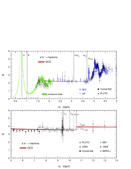
Figure 7: The spectrum of $e^{+}e^{-}$ annihilation into hadrons up to $\sqrt{s}=14\,\mbox{GeV}$. The cross-hatched band are the results of perturbation theory which agree nicely with the data in the continuum regions $2\,\mbox{GeV}<\sqrt{s}<3.1\,\mbox{GeV}$, $4.6\,\mbox{GeV}<\sqrt{s}<9.1\,\mbox{GeV}$, and $2\sqrt{s}>11.2\,\mbox{GeV}$. The resonances in the region $\sqrt{s}<2\,\mbox{GeV}$ and in the vicinity of the $c\bar{c}$ and $b\bar{b}$ thresholds are out the reach of perturbation theory. Taken from [141].

It is obvious from the figure that a spectrum calculated from a continuation of the practical OPE, $R=-\frac{1}{\pi}\mbox{Im}(Q^{2}=-s-i0)$, violates local quark-hadron duality considerably within the resonance regions since the contribution of power corrections arising from operators with anomalous dimensions alter the perturbative result in Fig. 7 only in a smooth way at finite $\sqrt{s}$.

(ii): The isovector-axialvector-induced spectrum (labelled by $A^{-}$) of $\tau$ decay into non-strange hadrons can be expressed as follows [179]

$$R_{A^{-}}(s) \equiv \frac{M_{\tau}}{6|V_{ud}|^{2}S_{EW}}\frac{B(\tau^{-}\to A^{-}\nu_{\tau})}{B(\tau^{-}\to e^{-}\bar{\nu}_{e}\nu_{\tau})}\times$$ (35)

$$\frac{dN_{A^{-}}}{N_{A^{-}}ds}\left(\left(1-\frac{s}{M_{\tau}^{2}}\right)\left(1+\frac{2s}{M_{\tau}^{2}}\right)\right)^{-1}\,$$

where $|V_{ud}|=0.9752\pm 0.0007$ is the CKM matrix element, $S_{EW}=1.0194\pm 0.004$ accounts for radiative electroweak corrections, $\frac{dN_{A^{-}}}{N_{A^{-}}ds}$ denotes the normalized invariant mass-squared distribution, and $M_{\tau}\sim 1.77\,$GeV is the mass of the $\tau$ lepton. In Fig. 8 the spectrum $R_{A^{-}}$ of $\tau$ decay as measured at LEP by the ALEPH collaboration [179] is shown.

Figure 8: Spectrum of axialvector-induced, $\tau$ decay into hadrons. Taken from [179].

Again, there is no way for a naive OPE continuation into the Minkowskian domain to generate the behavior of the spectrum around the $A_{1}$ resonance.

(iii): Experimental information on $B_{s}$-$\bar{B}_{s}$ mixing is not yet available, but it will be investigated by CDF in the near future [149]. A theoretical prediction resting on the assumption of local quark-hadron duality in the OPE approach exists at next-to-leading order in $\alpha_{s}$ [154]. Following [155] we briefly give some theoretical background on why $B_{s}$-$\bar{B}_{s}$ mixing can be a testing ground for the violation of local quark-hadron duality. Since $B_{s}$ may mix with its antiparticle $\bar{B}_{s}$ the two mass eigenstates $B_{H,L}$, which are linear combinations of $\bar{B}_{s}$ and $B_{s}$, have different masses, $\Delta m=M_{H}-M_{L}\not=0$, and different inclusive decay widths, $\Delta\Gamma=\Gamma_{H}-\Gamma_{L}\not=0$. $\Delta m$ and $\Delta\Gamma$ can be related to the dispersive (absorptive) part of the $B_{s}$-$\bar{B}_{s}$ mixing amplitude, $M_{12}$ ($\Gamma_{12}$), as follows

$$\Delta m=2|M_{12}|\,,\ \ \ \ \ \ \ \Delta\Gamma=2|\Gamma_{12}|\cos\phi\,.$$ (36)

Practically, we have $\Delta\Gamma=2|\Gamma_{12}|$ since the CP violating phase $\phi$ is very small in the Standard Model. By means of the optical theorem the Standard-Model expression for $\Delta\Gamma$ is

$$\Delta\Gamma=\left|\frac{1}{M_{B_{s}}}\mbox{Im}\left\langle\bar{B}_{s}|i\int d^{4}x\,T\,{\cal H}_{eff}(x){\cal H}_{eff}(0)|B_{s}\right\rangle\right|\,$$ (37)

where ${\cal H}_{eff}$ denotes the effective Hamiltonian mediating transition between $\bar{B}_{s}$ and $B_{s}$ in the Standard model after the heavy vector bosons $W^{\pm}$ and $Z_{0}$ have been integrated out using renormalization-group improved perturbation theory. The operators appearing in the decomposition of ${\cal H}_{eff}$ are normalized at a scale $\mu_{1}=O(m_{b})$. The variant of the OPE, which is used to estimate the right-hand side of Eq. (37), is an expansion in inverse powers of the $b$-quark mass $m_{b}$ - the so-called heavy quark expansion (HQE)[156]. Notice that this expansion relies on the validity of the HQE along the discontinuity in the Minkowskian domain. An experimental detection of a sizable CP asymmetry in the decays of $\bar{B}_{s}$ and $B_{s}$ would signal new physics. To test the Standard Model it is thus extremely important to have a good understanding of nonperturbative QCD effects and in particular of the validity of local quark-hadron duality in the use of HQE. To lowest order in $1/m_{b}$ one has

$$\left|\mbox{Im}\left\langle\bar{B}_{s}|i\int d^{4}x\,T\,{\cal H}_{eff}(x){\cal H}_{eff}(0)|B_{s}\right\rangle\right|=$$ (38)

$$= \frac{G_{F}^{2}m_{b}^{2}}{12\pi}|V_{cb}^{*}V_{cs}|^{2}\left|F\left(\frac{m_{c}^{2}}{m_{b}^{2}}\right)\left\langle\bar{B}_{s}|Q|B_{s}\right\rangle+F_{S}\left(\frac{m_{c}^{2}}{m_{b}^{2}}\right)\left\langle\bar{B}_{s}|Q_{S}|B_{s}\right\rangle\right|\,.$$

In Eq. (38) $G_{F}$ denotes the Fermi constant, $F$ and $F_{S}$ are the imaginary parts of the Wilson coefficients in the leading-order in $\alpha_{s}$ expansion, and $Q$($Q_{S}$) are the $\Delta B=2$ operators $\bar{s}_{i}\gamma_{\mu}(1\pm\gamma_{5})b_{i}\bar{s}_{j}\gamma^{\mu}(1\pm\gamma_{5})b_{j}$. The matrix elements of $Q$ and $Q_{S}$ are parametrized as

$$\left\langle\bar{B}_{s}|Q(\mu_{2})|B_{s}\right\rangle=\frac{8}{3}f_{B_{s}}^{2}M_{B_{s}}^{2}B(\mu_{2})\,,\ \ \ \ \left\langle\bar{B}_{s}|Q_{S}(\mu_{2})|B_{s}\right\rangle=-\frac{5}{3}f_{B_{s}}^{2}M_{B_{s}}^{2}\frac{M_{B_{s}}^{2}}{(m_{b}(\mu_{2})+m_{s}(\mu_{2}))^{2}}B_{S}(\mu_{2})\,$$ (39)

where $f_{B_{s}}$ and $M_{B_{s}}$ are the decay constant and the mass of the $B_{s}$ meson, and the masses $m_{b}(\mu_{2})$ and $m_{s}(\mu_{2})$ are defined in the $\overline{\mbox{MS}}$ scheme, and the normalization scale $\mu_{2}=O(m_{b})$. In the vacuum-saturation approximation the “bag” factors $B(\mu_{2}),B_{S}(\mu_{2})$ are equal to one.

At next-to-leading order in $\alpha_{s}$ there are already seven operators which describe nonlocal contributions to the transition. Including $m_{B}^{-1}$ corrections [157], the final answer for the quantity $\Delta\Gamma/\Gamma$, $\Gamma\equiv 1/2(\Gamma_{L}-\Gamma_{H})$, reads [155]

$$\frac{\Delta\Gamma}{\Gamma}=\left(\frac{f_{B_{s}}}{245\,\mbox{MeV}}\right)^{2}\,[(0.234\pm 0.035)B_{S}(m_{b})-0.080\pm 0.020]\,$$ (40)

where $m_{b}(m_{b})+m_{s}(m_{b})=4.3\,$GeV ($\overline{\mbox{MS}}$ scheme) and $m_{c}^{2}/m_{b}^{2}=0.085$ have been used. Due to its tiny numerical value the contribution $\propto B$ has been neglected in Eq. (40). With the result $f_{B_{s}}=(245\pm 30)$ MeV (for a QCD sum rule determination see for example [152]) of an unquenched lattice calculation [151] (two dynamical fermion flavors) and the result $B_{S}(m_{b})=0.87\pm 0.09$ of a quenched lattice calculation [153] one obtains (lattice errors added linearly)

$$\frac{\Delta\Gamma}{\Gamma}=0.12\pm 0.06\,.$$ (41)

In the limit of $N_{c}\to\infty$, where vacuum saturation is exact, and for $\Lambda_{QCD}\ll m_{b}-2m_{c}\ll m_{b}$ one can show that local duality holds exactly [158]. In this case the result is $\frac{\Delta\Gamma}{\Gamma}=0.18$ which is just in the upper error limit of Eq. (41). It is thus clear that a future experimental detection ($N_{c}=3$) of violations of local quark-hadron duality in the HQE for $\frac{\Delta\Gamma}{\Gamma}$ and/or of New Physics needs a much more precise (lattice)determination of $f_{B_{s}}^{2}B$ and $f_{B_{s}}^{2}B_{S}$, see for an unquenched, $N_{f}=2$ calculation of $B_{S}$ [150] where the error (and the central value) are reduced in comparison to the result of the quenched calculation in [153].

6.2 Quark propagation in an instanton background

Since no full, analytical solution of QCD exists, which would allow for a direct comparison of the OPE with the exact result (and make the OPE superfluous), one has to resort to models of the current-current correlator. It was proposed in [142] that in analogy to the cancellation of renormalon ambiguities, arising from a factorial growth of coefficients in the $\alpha_{s}$ expansion, by exponentially small terms $\mbox{e}^{1/\alpha_{s}}$, the OPE may (at best) be asymptotic in the according expansion in $\sim\frac{\Lambda_{QCD}}{Q}$. To make sense of it, one would then have to add exponentially small terms of the form $\mbox{e}^{Q/\Lambda_{QCD}}$ which possibly would cure the violation of local quark-hadron duality by practical OPEs.

A seemingly reasonable approach to see whether there is some truth in this proposal is to consider the quark propagation [122], inherent in a given correlator of currents with massless quarks, in a dilute-gas instanton-antiinstanton background [123, 124] or a general, (anti)selfdual background [127] (like a dilute gas of multiinstantons and multiantiinstantons).

Let us briefly review the calculation of the correlator of electric currents in a dilute-gas instanton-antiinstanton background as it was performed in [124] putting the (anti)instanton into the singular gauge. In the dilute-gas approximation it is only necessary to regard a single quark flavor $q$ of electric charge $Q$ - a sum over flavors can be performed at the end of the calculation. We consider the two-point correlator of the conserved current $j_{\mu}\equiv Q\bar{q}\gamma_{\mu}q$ in Euclidean position space

$$T_{\mu\nu}(x)=\left\langle Tj_{\mu}(x)j_{\nu}(0)\right\rangle\,.$$ (42)

Considering, in a first step, quark-propagation in the background of a single (anti)instanton and disregarding radiative corrections, the Lorentz-trace $T(x)=T^{\mu}_{\mu}(x)$ is simply given as

$$T_{\pm}(x,\Omega_{\pm})=-\sum_{F}\mbox{Tr}\,Q_{F}^{2}\gamma^{\mu}S_{\pm}^{F}(x,0,\Omega_{\pm})\gamma_{\mu}S_{\pm}^{F}(0,x,\Omega_{\pm})\,$$ (43)

where $S_{\pm}^{i}$ denotes the quark-propagator in the (anti)instanton background, the trace is over Dirac and color indices, the sum is over light quark flavors, and $\Omega_{\pm}$ denotes the collective parameters of the (anti)instanton. The propagators are expanded in mass $m_{i}$ around $m_{i}=0$

$$S_{\pm}(x,y,\Omega)=-\frac{\Psi_{0}(x)\Psi_{0}^{\dagger}(y)}{m}+\sum_{\lambda\not=0}\frac{\Psi_{\lambda}(x)\Psi_{\lambda}^{\dagger}(y)}{\lambda}+m\sum_{\lambda\not=0}\frac{\Psi_{\lambda}(x)\Psi_{\lambda}^{\dagger}(y)}{\lambda^{2}}+O(m^{2})\,$$ (44)

where $\lambda$ is a nonvanishing eigenvalue of the Dirac operator $i\gamma^{\mu}D_{\mu}$, and the subscript ‘0’ refers to the zero-mode contribution. It is important to keep the term linear in $m$ when calculating $T(x)$ in the limit $m\to 0$. The zero-mode part in Eq. (44) is given in terms of

$$(\Psi_{0}(x))_{\alpha,t}=\left(\frac{2}{\pi^{2}}\right)^{1/2}\frac{\rho_{\pm}}{((x-x_{\pm})^{2}+\rho_{\pm}^{2})^{3/2}}\left(i\gamma_{\mu}\hat{x}^{\mu}\gamma_{2}\frac{1}{2}(1\pm\gamma_{5})\right)_{\alpha,t}\,$$ (45)

where $\hat{x}$ denotes a 4D unit vector, and $\alpha(t)$ is a Dirac index (fundamental SU(2) color index). The $O(m^{0})$-part in Eq. (44), $S^{0}_{\pm}(x,y,\Omega_{\pm})$, can be written as [122]

$$S^{0}_{\pm}(x,y,\Omega_{\pm})=\gamma^{\mu}D^{x}_{\mu}\Delta_{\pm}(x,y,\Omega_{\pm})\frac{1}{2}(1\pm\gamma_{5})+(\Delta_{\pm}(x,y,\Omega_{\pm})D^{x}_{\mu}\gamma^{\mu})\frac{1}{2}(1\mp\gamma_{5})$$ (46)

where $\Delta_{\pm}(x,y,\Omega_{\pm})$ denotes the propagator of a scalar, color-triplet particle, and $(\Delta_{\pm}(x,y,\Omega_{\pm})D_{\mu}\gamma^{\mu})$ means that the covariant derivative acts from the right onto $\Delta_{\pm}(x,y,\Omega_{\pm})$. This propagator is explicitly known [122], in singular gauge it reads

$$\Delta_{\pm}(x,y,\Omega_{\pm}) = -\frac{1}{4\pi^{2}(x-y)^{2}}\left(1+\frac{\rho_{\pm}^{2}}{(x-x_{\pm})^{2}}\right)^{-1/2}\times$$ (47)

$$\left(1+\frac{\rho^{2}_{\pm}\sigma^{\mp}_{\mu}(x-x_{\pm})^{\mu}\sigma^{\pm}_{\nu}(y-x_{\pm})^{\nu}}{(x-x_{\pm})^{2}(y-x_{\pm})^{2}}\right)\left(1+\frac{\rho_{\pm}^{2}}{(y-x_{\pm})^{2}}\right)^{-1/2}\,$$

where $\sigma^{\pm}_{\mu}=(R_{ab}\,\sigma^{b},\mp i)_{\mu}$, $R_{ab}\in\,$SO(3) is a (constant) rotation matrix in adjoint SU(2) color space, $\sigma^{b}\,,(b=1,2,3),$ denoting the Pauli matrices, $\rho_{\pm}$ the (anti)instanton radius, and $x_{\pm}$ is the center of the (anti)instanton. The $O(m)$ contribution in Eq. (44), $S^{1}_{\pm}(x,y,\Omega)$, can simply be expressed as

$$S^{1}_{\pm}(x,y,\Omega)=m\int d^{4}z\,S^{0}_{\pm}(x,z,\Omega_{\pm})S^{0}_{\pm}(z,y,\Omega_{\pm})\,.$$ (48)

Inserting the zero-mode expression (45), and the zeroth- (first)- order in $m$ expressions Eq. (46) (Eq. (48)) into Eq. (43) and only considering the part, which survives the limit $m\to 0$, averaging over the color orientations of the instanton embedding into SU(3), subtracting the free current correlator $T_{0}$, performing the integration over (anti)instanton centers and radii over the remainder, and taking into account the contribution from instantons and antiinstantons in this part, one arrives at the following expression [124]

$$\delta T(x)=(\sum_{F}Q_{F}^{2})\frac{36}{\pi^{2}}\int\frac{d\rho}{\rho^{5}}D(\rho)\frac{\rho^{4}}{x^{4}}\partial_{x^{2}}\left(\frac{1}{x^{2}}\frac{1}{(1+4\rho^{2}/x^{2})^{1/2}}\,\log\frac{(1+4\rho^{2}/x^{2})^{1/2}+1}{(1+4\rho^{2}/x^{2})^{1/2}-1}\right)\,$$ (49)

where $D(\rho)$ denotes the instanton density at one-loop perturbation theory (only gluonic fluctuations),

$$D(\rho)\equiv\frac{0.1}{\rho^{5}}\left(\frac{8\pi^{2}}{g^{2}(\Lambda_{QCD}\rho)}\right)^{6}\exp\left(\frac{-8\pi^{2}}{g^{2}(\Lambda_{QCD}\rho)}\right)\,$$ (50)

which can be interpreted as the number of instantons of size between $\rho$ and $\rho+d\rho$ per unit space-time volume.

After separating off a factor $\frac{3}{4\pi^{2}}q^{2}$ (arising from the transverse tensor structure) in the Fourier transform of the entire correlator $T_{0}+\delta T(x,\rho)$ and after accounting for the Gaussian integration over fermionic fluctuations around the (anti)instanton we have

$$\bar{T}(Q^{2}) = -\frac{4\pi^{2}}{3Q^{2}}T(Q^{2})$$ (51)

$$= (\sum_{F}Q_{F}^{2})\left(\log\frac{Q^{2}}{\mu^{2}}+16\pi^{2}\int\frac{d\rho}{\rho}D(\rho)\Delta(\rho)\left[\frac{1}{3(Q\rho)^{4}}-\frac{1}{(Q\rho)^{2}}\int_{0}^{1}du\,K_{2}\left(\frac{2Q\rho}{\sqrt{1-u^{2}}}\right)\right]\right)\,$$

where $\Delta(\rho)$ denotes the associated (dimensionless) fermion determinant [125], and $K_{2}$ is a McDonald function. The integral over $\rho$ is cut off at small $\rho$ by the fermion determinant. For large $\rho$ it is ill-behaved which signals that the dilute-gas approximation as well as the one-loop perturbative treatment of fluctuations breaks down. One usually introduces an upper cutoff $\rho_{c}\sim\Lambda_{QCD}^{-1}$ by hand.

Clearly, there is a dimension-four power correction arising from the first part of the integrand in Eq. (51) which can be associated with the gluon condensate. The second part of the integrand, however, is not a power correction. For asymptotic momenta $Q\to\infty$ it falls off exponentially and can be taken as an indication for the searched-for exponentially small terms needed to cure the OPE. The reader may wonder why there is only a dimension-four power correction in Eq. (51). To answer this, let us recall that the appearance of dimension-six condensates is associated with radiative corrections - the prefactor $\alpha_{s}$ before the four-quark operators refers to a gluon exchange initiated by the current-induced quarks. On our above treatment of quark propagation, however, we did only consider radiative corrections to the background-field but not to the quark propagation in this background.

One may now continue Eq. (51) to the Minkowskian domain and determine its imaginary part to give a prediction for the ratio $R=-\frac{1}{\pi}\mbox{Im}(Q^{2}=-s-i0)$ in Eq. (34).

The result is

$$\bar{R}(E) = \frac{1}{\sum_{F}Q_{F}^{2}}\left(R_{0}(E)+R^{I}(E)\right)$$ (52)

$$= 1+\frac{16\pi^{2}}{3}\int\frac{d\rho}{\rho}\frac{D(\rho)}{(E\rho)^{2}}\Delta(\rho)\left[\frac{1}{\rho^{2}}\delta(E^{2})+\frac{3}{2(E\rho)^{2}}\int_{0}^{1}du\,J_{2}\left(\frac{2E\rho}{\sqrt{1-u^{2}}}\right)\right]\,$$

where $E\equiv\sqrt{s}$, $R_{0}(E)$ and $R^{I}(E)$ denote the free particle and the instanton induced parts, respectively, and $J_{2}$ is a Bessel function. In [142] the product $\frac{D(\rho)}{(E\rho)^{2}}\Delta(\rho)$ was approximated by the simplest possible form

$$\frac{D(\rho)}{(E\rho)^{2}}\Delta(\rho)=d_{0}\rho_{0}\,\delta(\rho-\rho_{0})\,$$ (53)

where a value $\rho_{0}=1.15\,\mbox{GeV}^{-1}$ and $d_{0}=9\times 10^{-2}$ was adopted . A comparison of the function $\bar{R}(E)$ in (53) and the experimental results for $\bar{R}(E)$ is presented in Fig 9. It is obvious that the part in Eq. (52) not contained in the practical OPE is responsible for the resonance-like behavior at low $E$. Although quantitatively the two plots in Fig. 9 differ - after all it is clear that an incomplete dilute-gas approximation, recall the bold choice of the instanton weight in Eq. (53), is not a good approach - there is at least some qualitative agreement.

Figure 9: Experimental results for $\bar{R}(E)$ (right panel) and the result of Eq. (52) obtained in the instanton model (left panel). The dashed line corresponds to the parton-model result. Plots taken from [142].

6.3 Duality analysis in the ’t Hooft model

QCD in two dimensions (QCD₂) considered in the limit $N_{c}\to\infty$ with $g^{2}N_{c}$ fixed - the so-called ’t Hooft model [159] - is exactly solvable. At finite but large $N_{c}$ a well controlled expansion in powers of $1/N_{c}$ is available. For this reason it is the ideal testing ground for questions on local quark-hadron duality, namely, at large external momenta the practical OPE of some polarization operator (current correlator) can directly be compared with the asymptotically exact result, and duality violating contributions can be identified. A vast literature exists on the subject, see for example [161, 162, 163, 164, 165, 167, 169, 168, 170, 171, 172, 173, 174], and not all contributions can be explicitly referred to here. A review, which also discusses the string interpretation of the ’t Hooft-model results, exists [175]. During the ten years or so the interest in the ’t Hooft model was boosted by questions of duality-violations in the weak decay of heavy quark flavors, see for example [167, 170, 169, 171, 170, 172], by the necessity to check the reliability of lattice calculations, see [173, 174], by the need to estimate higher-twist corrections to parton distribution functions [165]. A dynamical understanding of chiral symmetry breaking in two dimensions was obtained relatively early [164]. In this section we are mainly concerned with duality violations in spectral functions based on the OPEs of current correlators when allowing for $1/N_{c}$ corrections.

6.3.1 Prerequisites

Before going into the technical details of duality violations in the ’t Hooft model we will here give a brief introduction into this model [159].

One considers the usual QCD Lagrangian

$${\cal L}=-\frac{1}{4}G^{a}_{\mu\nu}G_{a}^{\mu\nu}+\sum_{F}\bar{q}^{F}(i\gamma^{\mu}D_{\mu}-m_{F})q^{F}\,.$$ (54)

Spacetime is two dimensional, the gauge group is U($N_{c}$) instead of SU($N_{c}$), and the gauge coupling $g$ has the dimension of a mass. Conveniently, one works in light-cone coordinates $x^{\pm}=\frac{1}{\sqrt{2}}\left(x^{1}\pm x^{0}\right)$ and $A_{\pm}=\frac{1}{\sqrt{2}}\left(A_{1}\pm A_{0}\right)$ where $x^{1}=x_{1}$ and $x^{0}=-x_{0}$. Imposing the (ghost-free) light-cone gauge $A_{-}=A^{+}=0$, one has $G_{+-}=-\partial_{-}A_{+}$ and Eq. (54) reduces to

$${\cal L}=\frac{1}{4}(\partial_{-}A_{+}^{a})^{2}+\sum_{F}\bar{q}^{F}(i\gamma^{\mu}\partial_{\mu}-m_{F}+g\gamma_{-}A_{+})q^{F}\,.$$ (55)

Taking $x^{+}$ as the new time direction, the field $A_{+}^{a}$ has no time-derivatives, and thus it is not dynamical. It will provide for a static Coulomb force between the quarks. Since $\gamma_{-}^{2}=\gamma_{+}^{2}=0$, $\gamma_{+}\gamma_{-}+\gamma_{-}\gamma_{+}=2$, and since the vertex in Eq. (55) comes with a $\gamma_{-}$ one can eliminate the gamma matrices from the Feynman rules. Suppressing color indices, the gluon propagator is $1/k^{2}_{-}$, the quark propagator is $k_{-}/(2k_{+}k_{-}-m_{F}^{2}+i\epsilon)$, and the vertex is $2g$. It was shown in [160] that in the limit $N_{c}\to\infty$ with $g^{2}N_{c}$ fixed only planar diagrams with no fermion loops like the ones in Fig. 10 survive in the calculation of any amplitude.

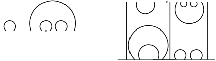
Figure 10: Planar diagrams contributing to the quark self-energy and the quark-antiquark scattering amplitude. Thick lines denote gluon propagators (not dressed in the limit $N_{c}\to\infty$, $g^{2}N_{c}$ fixed) and thin, arrowed lines propagators refer to quark propagators.

Due to this extreme simplification the equation for the quark self-energy (the rectangular blob in Fig. 11) can be written in untruncated form.

To solve this equation requires, in intermediate steps, the introduction of a symmetric ultra-violet cutoff as well as an infra-red cutoff. The former is a consequence of the strong gauge fixing and has no physical interpretation. The removal of the latter in the final result, which does not depend on the ultra-violet cutoff, shifts the pole of the quark-propagator to infinity - one concludes that the spectrum has no single quark state. To determine the spectrum of quark-antiquark bound states one has to look at the homogeneous Bethe-Salpeter equation as depicted in Fig. 12.

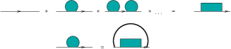
Figure 11: The Dyson series for the quark self-energy (upper figure) and the equation which determines it in the limit $N_{c}\to\infty$, $g^{2}N_{c}$ fixed.

Exploiting that the Coulomb force is instantaneous to separate the loop integrals and introducing the following dimensionless quantities (compare with Fig. 12)

$$\gamma^{2}\equiv m^{2}/\mu^{2}\,,\ \ \ \ \mu_{n}^{2}\equiv m_{n}^{2}/\mu^{2}\,,\ \ \ \ x\equiv p_{-}/r_{-}\,,$$ (56)

where $\mu\equiv(g^{2}N_{c})/\pi$ and $m_{n}$ is the mass of the $n$th meson, one obtains the ’t Hooft equation for the mesonic wave functions $\phi_{n}(x)$

$$\mu_{n}^{2}\phi(x)=\frac{(\gamma^{2}-1)\phi_{n}(x)}{x(1-x)}-P\int_{0}^{1}dy\,\frac{\phi_{n}(y)}{(x-y)^{2}}\,$$ (57)

with $P$ denoting principle-value integration, $P\left[1/(x-y)^{2}\right]\equiv\lim_{\epsilon\to 0}\frac{1}{2}[1/(x-y+i\epsilon)^{2}+1/(x-y-i\epsilon)^{2}]$. In writing Eq. (57) we have assumed the masses of the participating quark and antiquark to be equal, $m_{F}=m_{\bar{F}}=m$.

Figure 12: Homogeneous Bethe-Salpeter equation which determines the spectrum of meson states in the limit $N_{c}\to\infty$, $g^{2}N_{c}$ fixed.

It was shown in [159] that the “Hamiltonian” defined by the right-hand side of Eq. (57) is hermitian and positive definite (finite quark mass, $\gamma>0$) on the Hilbert space of functions which vanish at x=0,1 like $x^{\beta},(1-x)^{\beta}$ where $\beta$ is a root of $\pi\beta\cot(\pi\beta)=1-\gamma$. The spectrum is discrete and is for large $n$ approximated by $\phi_{n}\sim\sqrt{2}\sin(\pi nx)$ and $\mu_{n}^{2}=\pi^{2}n$. For $\gamma=0$ the lowest meson mass vanishes, the associated wave function is $\phi_{0}=1$.

Since the spectrum is real and positive definite resonances do not decay into one another - their width is zero. At large $s$ (or $n>n_{0}$) the spectral function of a correlator $T$ of currents, which couple to all meson states equally, is therefore well approximated by equidistant, zero-width spikes:

$$\rho(s)=\mbox{Im}\,T=\mbox{const}\frac{N_{c}}{2}\sum_{n>n_{0}}^{\infty}\delta\left(\frac{s}{\pi^{2}\mu}-n\right)\,.$$ (58)

6.3.2 Current-current correlator and spectral function at $O(1/N_{c})$

Our discussion of local duality violation of current-current correlators in QCD₂ beyond the limit $N_{c}\to\infty$ relies on work [168] which uses the older results in [161, 162, 163].

At finite $N_{c}$ the quark-antiquark bound states of the ’t Hooft model are unstable. For a decay $a\to b+c$ the width $\Gamma_{a}$ at $O(1/N_{c})$ is given as [161, 162, 163]

$$\Gamma_{a}=\frac{1}{8m_{a}}\sum_{b}\sum_{c}\frac{g_{abc}^{2}}{\sqrt{I(m_{a},m_{b},m_{c})}}\,,$$ (59)

where $I(m_{a},m_{b},m_{c})=1/4[m_{a}^{2}-(m_{b}+m_{c})^{2}][m_{a}^{2}-(m_{b}-m_{c})^{2}]$ and the meson coupling is given as

$$g_{abc}=32\mu^{2}\sqrt{\frac{\pi}{N_{c}}}\left[1-(-1)^{\sigma_{a}+\sigma_{b}+\sigma_{c}}\right](f_{abc}^{+}+f_{abc}^{-})\,.$$ (60)

The parity of the $a$th meson is $\sigma_{a}$. The quantities $f_{abc}^{\pm}$ are constants for on-shell decay. They are given by overlap integrals between the meson wave functions $\phi_{a,b}$ and the Bethe-Salpeter kernel, see [168]. For lack of better analytical knowledge Eq. (59) was used in [168] with the asymptotic spectrum, even for $a,b,c\leq n_{0}$. For small $a$ one should not trust this approximation. For an investigation of duality violating components at large $Q$ it is, however, justified. A numerical evaluation of Eq. (59) and a subsequent fit to a square-root dependence yields the following estimate

$$\Gamma_{n}=\frac{(A=15\pm 1.5)\mu}{\pi^{2}N_{c}}\sqrt{n}\left[1+O(1/n)\right]\,.$$ (61)

This knowledge of the dependence of width on $n$ can be exploited to estimate the correlator $T(q^{2})=i\int d^{2}x\,\mbox{e}^{iqx}\left\langle Tj(x)j(0)\right\rangle$ of the scalar current $j=\bar{q}q$. In the limit $N_{c}\to\infty$ it is given as

$$T(q^{2})=-\sum_{n=0}^{\infty}\frac{g_{n}^{2}}{q^{2}-m_{n}^{2}+i\epsilon}\,.$$ (62)

Requiring this to match the leading perturbative order for $-q^{2}=Q^{2}\to\infty$ (duality in mesonic and quark description of asymptotic freedom in $T(Q^{2}\to\infty)$), one obtains [161]

$$g_{n}^{2}=N_{c}\pi\mu^{2}\,,\ \ \ \ \ \ \ \ (n\ \mbox{odd})\,.$$ (63)

Figure 13: The spectral density $\mbox{Im}\,T(s)$ in the ’t Hooft model with the leading $1/N_{c}$ contribution to the resonance widths included. The center-of-mass momentum $s$ is given in units of $2\pi^{2}\mu^{2}$. Plot taken from [168].

Inserting Eq. (63) into Eq. (62) and taking the imaginary part, one arrives at an expression like in Eq. (58). By means of a dispersion relation one can define Im $T(q^{2}>0)$ to $T(q^{2})$ everywhere in the complex $q^{2}$-plane, up to a constant. This gives [168]

$$T(q^{2})-T(0)=-\frac{N_{c}}{2\pi}\,\psi(\sigma)\,,\ \ \ \ \sigma=\frac{Q^{2}}{2\pi^{2}\mu^{2}}+\frac{1}{2}\,$$ (64)

where $\psi(\sigma)$ denotes the logarithmic derivative of Euler’s Gamma function. So far we have discussed the narrow-width case ($N_{c}\to\infty$). The finite-width case is treated in the Breit-Wigner approach by replacing $q^{2}-m_{n}^{2}+i\epsilon\to q^{2}-m_{n}^{2}+\Sigma(q^{2})$ in Eq. (62). Since $\mbox{Im}\,\Sigma(q^{2}=m_{n}^{2})=m_{n}\Gamma_{n}=\frac{Am_{n}^{2}}{\pi^{3}N_{c}}$ one may take $\Sigma(Q^{2})=\frac{A}{\pi^{4}N_{c}}Q^{2}\log\frac{Q^{2}}{2\pi^{2}\mu^{2}}$. As a result, the correlator with $1/N_{c}$ corrections in the widths included reads

$$T(q^{2})-T(0)=-\frac{1}{1-A/(\pi^{4}N_{c})}\frac{N_{c}}{2\pi}\,\psi(\tilde{\sigma})\,,\ \ \ \ \tilde{\sigma}=\left(\frac{Q^{2}}{2\pi^{2}\mu^{2}}\right)^{-A/(\pi^{4}N_{c})+1}+\frac{1}{2}\,.$$ (65)

Fig. 13 shows the spectral density $\mbox{Im}\,T(s)$. The broadening of the resonances with increasing $s$ is clearly visible. How does this result compare with the practical OPE? The OPE corresponding to Eq. (65) is known to be the following (asymptotic) expansion [168]

$$T(q^{2})-T(0)=-\frac{1}{1-A/(\pi^{4}N_{c})}\frac{N_{c}}{2\pi}\,\left[\log\tilde{\sigma}+\frac{1}{\tilde{\sigma}}-\sum_{n=1}(-1)^{n-1}\frac{B_{n}\tilde{\sigma}^{-2n}}{2n}\right]\,.$$ (66)

The Bernoulli numbers behave at large $n$ as $B_{n}\sim(2n)!$ which shows that the expansion is asymptotic. The variable $\tilde{\sigma}$ can be obtained from $\sigma$ by replacing $Q^{2}\to z$. Consequently, the powers in $Q^{-2}$ in Eq. (66) are slightly displaced at finite $N_{c}$ as compared to their integer values at $N_{c}\to\infty$. Expanding in this deviation $\alpha=\frac{A}{\pi^{4}N_{C}}$, this introduces logarithmic corrections:

$$\left(1/Q^{2}\right)^{2n-\alpha}\to\left(1/Q^{2}\right)^{2n}(1+\alpha\log Q^{2}+\cdots)\,.$$ (67)

The logarithms in Eq. (67) lead to smooth contributions to the spectral density at finite $s$ which, however, vanish in the limit $N_{c}\to\infty$. A direct (not using the asymptotic expansion (66)) calculation of the spectral density reveals an oscillating component $2\exp[-\alpha s/\mu^{2}]\cos[s/(\pi\mu^{2})]$ for $\alpha s\gg\mu^{2}$ which, however, is not suppressed by $1/N_{c}$. This contribution signals the violation of local quark-hadron duality.

6.3.3 Decays of heavy mesons

As a final testing ground for the study of the violation of local quark-hadron duality in the ’t Hooft model we will now discuss the weak decay of heavy-light mesons. There has been a rather high research activity within the last few years investigating the issue of both global, see for example [167], and local duality, see for example [170, 171, 169, 172]. This is natural since important lessons for the (3+1) dimensional case, which is targeted by present experiments at the $B$ factories, can be drawn.

Our discussion mainly follows [170]. To describe weak decays the ’t Hooft-model Lagrangian has to be supplemented by a weak-interaction part. Effectively, we can take it to be of the current-current form

$${\cal H}_{eff}^{V}=\frac{G}{\sqrt{2}}\left(\bar{q}\gamma_{\mu}Q\right)\left(\bar{\psi}_{a}\gamma^{\mu}\psi_{b}\right)\,$$ (68)

for two vector currents since the axial current reduces to the vector current in (1+1) dimensions. The constant $G$ is the 2D analogue of the Fermi coupling in 4D. By means of the optical theorem the inclusive decay with $\Gamma_{H_{Q}}$ reads

$$\Gamma_{H_{Q}}=\mbox{Im}\frac{i}{M_{H_{Q}}}\int d^{2}x\left\langle H_{Q}|T{\cal H}_{eff}^{V}(x){\cal H}_{eff}^{V}(0)|H_{Q}\right\rangle\,$$ (69)

where $H_{Q}$ denotes the state with the heavy meson at rest. Depending on whether we describe semileptonic or hadronic decay the fields ${\psi}_{a,b}$ in Eq. (68) are either leptonic fields or quark fields. We only discuss the case where $m_{\psi}=0$. As was shown in [170], the current $\bar{\psi}_{a}\gamma^{\mu}\psi_{b}$ can be substituted by $\epsilon^{\mu\nu}\partial_{\nu}\phi/\sqrt{\pi}$ where $\phi$ denotes a pseudoscalar, massless field . The corresponding lowest-order diagram for the transition amplitude is shown in Fig. 14. The parton-model result is

$$\Gamma_{Q}=\frac{G^{2}}{4\pi}\frac{m_{Q}^{2}-m_{q}^{2}}{m_{Q}}\,$$ (70)

and can be obtained by replacing the heavy meson by the heavy quark to be able to calculate the average over the operator $T^{0}=c^{0}_{\bar{Q}Q}\bar{Q}Q$ with $2\mbox{Im}\,c^{0}_{\bar{Q}Q}=\Gamma_{Q}$.

Figure 14: Lowest-order diagram for the transition amplitude in Eq. (69). The wave line represents the propagation of the pseudoscalar massless particle which is composed of $\bar{\psi}_{a}$ and $\psi$. Taken from [170].

Going beyond the parton-model approximation, the (spacetime integral of the) operator $\bar{Q}Q$ needs to be expanded in powers of $1/m_{Q}$. Up to $O(1/m_{Q}^{3})$ one obtains [170]

$$\frac{\left\langle H_{Q}|\bar{Q}Q|H_{Q}\right\rangle}{2M_{H_{Q}}}=1-\frac{1}{2m_{Q}^{2}}\frac{\left\langle H_{Q}|\bar{Q}(-D_{1}^{2})Q|H_{Q}\right\rangle}{2M_{H_{Q}}}+\frac{g^{2}}{2m_{Q}^{3}}\frac{\left\langle H_{Q}|\bar{Q}\gamma_{\mu}t^{a}\sum_{q}\bar{q}\gamma^{\mu}t^{a}q|H_{Q}\right\rangle}{2M_{H_{Q}}}+O\left(\frac{1}{m^{4}_{Q}}\right)\,.$$ (71)

Including first-order in $g^{2}$ radiative corrections to the coupling $Qq\phi$ simply amounts to a shift of the quark masses: $m_{Q,q}^{2}\to m_{Q,q}^{2}-\beta^{2}$ where $\beta^{2}=\lim_{N_{c}\to\infty}\frac{g^{2}}{2\pi}N_{c}<\infty$ denotes the ’t Hooft coupling. This is actually true to all orders [170]. As a consequence, we have to all orders that $2\,\mbox{Im}\,c_{\bar{Q}Q}=\frac{G^{2}}{4\pi}\frac{m_{Q}^{2}-m_{q}^{2}}{\sqrt{m_{Q}^{2}-\beta^{2}}}$. Under radiative corrections the expansion of $c_{\bar{Q}Q}\bar{Q}Q$ up to $O(1/m^{4}_{Q})$ thus is entirely due to the one of the operator $\bar{Q}Q$, see Eq. (71). As far as the first subleading, dimension two, four-fermion operator $O_{4q}=\bar{Q}\Gamma_{1}Q\bar{q}\Gamma_{2}q$ - $\Gamma_{1,2}$ denoting color and spinor matrices - is concerned it can be shown that its Wilson coefficient $c_{4q}$ does not develop an imaginary part at leading order in $g$ and at one loop. Thus this operator does not contribute to the total width up to $O(1/m_{b}^{3})$. There is a contribution of $O(1/m_{b}^{5})$ at two loop, and hence we have up to $O(1/m_{b}^{4})$

$$\Gamma_{H_{Q}}=\frac{G^{2}}{4\pi}\frac{m_{Q}^{2}-m_{q}^{2}}{\sqrt{m_{Q}^{2}-\beta^{2}}}\left[\frac{\left\langle H_{Q}|\bar{Q}Q|H_{Q}\right\rangle}{2M_{H_{Q}}}+O\left(\frac{1}{m_{Q}^{5}}\right)\right]\,.$$ (72)

Eq. (72) can be compared with the following result of a calculation obtained by using the ’t Hooft equation (now with $m_{Q}$ and the mass of the spectator quark $m_{sp}\not=m_{Q}$) [170]

$$\Gamma_{H_{Q}}=\frac{G^{2}}{4\pi}\frac{m_{Q}^{2}-m_{q}^{2}}{m_{Q}}\left[\frac{m_{Q}}{M_{H_{Q}}}\int_{0}^{1}\frac{dx}{x}\,\phi^{2}_{H_{Q}}(x)+O\left(\frac{1}{m_{Q}^{5}}\right)\right]\,.$$ (73)

Writing the operator $\bar{Q}Q$ in terms of quark-components in the light-cone formalism and absorbing renormalization factors, the matrix element in Eq. (72) can be expressed as a functional of $\phi_{H_{Q}}$ such that Eq. (73) is reproduced. Up to $O(1/m_{Q}^{4})$ the OPE prediction matches the expansion of the exact result. Also, the absence of a $1/m_{b}$ correction, found by analyzing the OPE, can directly be verfied using the HQE of the ’t Hooft equation in the approach of Ref. [166].

To derive Eq. (73) a sum over exclusive widths $\Gamma_{n}$ for the decay into the $n$th meson had to be performed from which the off-shell part ($m_{n}>M_{H_{Q}}$) had to be subtracted afterwards. It can be estimated that the analytic part of the latter term is $O(1/m_{Q}^{5})$. If there is a nonanalytic violation of local duality $\Delta\Gamma^{osc}$ it must reside in the sum with $m_{n}>M_{H_{Q}}$. An estimate of $\Delta\Gamma^{osc}$ was made in [170] for $m_{sp}\leq\beta$. In Fig. 15 $\Delta\Gamma^{osc}$ is shown as a function of the heavy meson mass.

Figure 15: The oscillatory part of $\Gamma_{H_{Q}}$ represented as the ratio $\Delta\Gamma^{osc}/(G^{2}\beta)$ versus the ratio $M^{2}_{H_{Q}}/(\pi^{2}\beta^{2})$. Taken from [170].

The relative amplitude of the oscillatory part can be estimated as

$$\left|\frac{\Delta\Gamma^{osc}}{\Gamma_{Q}}\right|_{\tiny\mbox{max}}\sim\frac{3\pi^{4}}{2}\left(\frac{\beta}{M_{H_{Q}}}\right)^{9}\,,$$ (74)

and hence it is strongly power-suppressed in the weak-coupling limit $M_{H_{Q}}\gg\beta$.

To conclude, there is definitely an oscillatory, duality violating component in the inclusive decay width for the semileptonic or hadronic decay of a heavy meson in QCD₂ considered in the limit $N_{c}\to\infty$, $g^{2}N_{c}$ fixed. It is strongly power-suppressed for $M_{H_{Q}}\gg\beta$.

7 OPE and nonperturbative nonlocality

In the last section we used field-theory models, which are not too far from first-principle, realistic QCD, to pin down the terms absent in practical OPEs that lead to a violation of local quark-hadron duality. This section approaches the problem from a more phenomenological side. By relating moments of hadronic light-cone wave functions (also called distribution amplitudes (DAs)) to the OPE representation of an appropriate vacuum correlator, thereby gainig experimentally testable information on the wave functions in terms of perturbative QCD and condensates [184, 185], a phenomenological analysis of the validity of the OPE can be performed. Allowing for deviations from the locality of condensates - a possibility discussed since the early days of QCD sum rules[181, 243, 43, 200, 145, 146, 147, 182, 73, 222] - strongly suggests that a truncated, practical OPE is insufficient to reproduce the experimentally favored shapes of DAs [200]. The same conclusion can be reached by a comparison of a re-ordering of the OPE, which sums up an infinite series of operators of increasing powers in covariant derivatives, with experimental data.

7.1 Distribution amplitudes and photon-photon annihilation

Before going into the details of the sum-rule approaches of [185] and [200] to the determination of DAs we will set the stage by explaining and applying them in (3+1) dimensions. In the 2D case we have already encountered them in our discussion of the ’t Hooft model.

In the calculation of exclusive processes with a large momentum transfer - like the hadronic decay of heavy mesons or the photon-photon annihilation into hadrons - mesonic DAs appear quite naturally. They were introduced to separate nonperturbative large-distance physics from the perturbatively accessible small-distance physics in the calculation of transition amplitudes [186, 190, 187] (an exhaustive discussion is given in [190]). In general, the DA of a hadron decomposes into a part describing the valence quark and/or gluon content and into parts associated with the contribution of higher, color-singlet Fock states. For example, the $\pi^{+}$ wave function $\varphi(x,\mu^{2})$ associated with the lowest-twist, nonlocal operator and with the lowest Fock state is defined as

$$\left\langle 0\left|\bar{d}(z)\gamma_{\nu}\gamma_{5}{\cal P}\exp\left[ig\int_{-z}^{z}dy^{\mu}\,A_{\mu}\right]u(-z)\right|\pi^{+}(q)\right\rangle_{\mu^{2}}$$

$$= \sum_{n=0}^{\infty}\frac{(-1)^{n}}{n!}\left\langle 0\left|\bar{d}(z)\gamma_{\nu}\gamma_{5}\left(z^{\mu}[\overrightarrow{D}_{\mu}-\overleftarrow{D}_{\mu}]\right)^{n}u(0)\right|\pi^{+}(q)\right\rangle_{\mu^{2}}$$

$$= iq_{\nu}\,\phi(z\cdot q,\mu^{2})+\cdots\,,$$

$$\phi_{\pi}(z\cdot q,\mu^{2}) = \int_{-1}^{+1}d\xi\,\mbox{e}^{i\xi(z\cdot q)}\varphi_{\pi}(\xi,\mu^{2})\,$$ (75)

where the separation $2z$ is light-like, $z^{2}=0$, the sum is over even $n$, and ${\cal P}$, $\mu$ denote path ordering and the normalization point of the operators, respectively. In Eq. (7.1) only the function $\phi_{\pi}(z\cdot q,\mu^{2})$ associated with the valence quark distribution is explicitly indicated, paranthesis refer to higher Fock states. Writing $\xi=2x-1$, the quantity $x$ or $(x-1)$ is the fraction of longitudinal pion momentum carried by the quark or antiquark, respectively. The DA $\varphi_{\pi}(\xi,\mu^{2})$ is interpreted as the integral of the full Bethe-Salpeter wave function over transverse momenta $k_{\perp}$ down to $k_{\perp}\sim\mu$. The dependence on the cutoff $\mu$ in $\varphi_{\pi}(\xi,\mu^{2})$ can most conveniently be obtained by expanding into eigenfunctions of the evolution kernel obtained by considering one-gluon-exchange ladder diagrams which contribute perturbatively to the wave function [186]. The expansion is given as

$$\varphi_{\pi}(\xi,\mu^{2})=(1-\xi^{2})\sum_{n=0}^{\infty}a_{n}C_{n}^{3/2}(\xi)\left[\log\left(\frac{Q^{2}}{\Lambda_{QCD}^{2}}\right)\right]^{-\gamma_{n}}\,$$ (76)

where the eigenvalue $\gamma_{n}$ is given as $\gamma_{n}=\frac{4}{3b}\left[1-2/((n+1)(n+2))+4\sum_{l=2}^{n+1}1/l\right]$, and $b=11-\frac{2}{3}$ is the first coefficient of the QCD beta function. Due to the orthonormality (with weight $(1-\xi^{2})$) of the Gegenbauer polynomials $C_{n}^{3/2}$ on [-1,1] the expansion coefficients are simply given as $a_{n}=\int_{-1}^{1}d\xi\,C_{n}^{3/2}(\xi)\varphi(\xi,\mu_{0}^{2})$.

Figure 16: Diagram contributing to the hard scattering amplitude in $\gamma\gamma^{*}\to\pi^{0}$ to lowest order in $\alpha_{s}$. Wiggly lines denote photons, a solid line a quark or an antiquark.

Let us now discuss two applications of DAs. We first consider the annihilation of two photons into hadrons, $\gamma\gamma\to X_{h}$. One of the photons either is highly virtual or it is real but incident under a large angle $\theta_{c.m.}$ in the center-of-mass frame. This is described in terms of a convolution of a hard scattering amplitude $T_{H}$, calculable in perturbation theory (see Figs. 16,17), with the DAs of the hadrons produced. For example, for the process $\gamma\gamma^{*}\to\pi^{0}$ this arises by considering a partial, perturbative contraction of quark fields in the amplitude $\left\langle\pi^{0}|j_{\mu}(y)j_{\mu}(0)|0\right\rangle$, yielding propagator lines to which the external photons couple, and a soft remainder which in lowest-order twist is given by Eq. (76). The vertex $\Gamma_{\mu}$ for this process is

$$\Gamma_{\mu}=-ie^{2}F_{\pi\gamma}(Q^{2})\,\varepsilon_{\mu\nu\rho\sigma}p^{\nu}\epsilon^{\rho}q^{\sigma}\,$$ (77)

where $p$ is the pion’s momentum, $\epsilon^{\rho}$ the polarization vector of the real photon, $q$ (with $q^{2}=-Q^{2}$) the momentum of the virtual photon, and $F_{\pi\gamma}(Q^{2})$ the photon-pion transition form-factor. The latter can be written as the convolution of hard scattering amplitude (see Fig. 16) with the pion wave function. To zeroth order in $\alpha_{s}$ we have

$$F_{\pi\gamma}(Q^{2})=\frac{2}{\sqrt{3}Q^{2}}\int_{0}^{1}dx\,\frac{\varphi_{\pi}(x,Q^{2}_{x})}{x(1-x)}\,$$ (78)

where $Q_{x}=\mbox{min}(x,1-x)\,Q$. The amplitude ${\cal M}_{\lambda\lambda^{\prime}}$ for the process $\gamma\gamma\to\pi^{+}\pi^{-}$ at large angle $\theta_{c.m.}$ is given as [189]

$${\cal M}_{\lambda\lambda^{\prime}}=\int_{0}^{1}dx_{1}\,\int_{0}^{1}\,dx_{2}\,\varphi_{\pi}(x_{1},Q^{2}_{x_{1}})\varphi_{\pi}(x_{2},Q^{2}_{x_{2}})\times T_{\lambda\lambda^{\prime}}(x_{1},x_{2},s,\theta_{c.m.})\,$$ (79)

where $\lambda,\lambda^{\prime}$ denote the helicities $+$ or $-$ of the photons and $Q_{x_{1}}\sim\mbox{min}(x_{1},1-x_{1})\sqrt{s}|\sin\theta_{c.m.}|$ (accordingly for $Q_{x_{2}}$).

Figure 17: Diagrams contributing to $T_{\lambda\lambda^{\prime}}$ of Eq. (79) to lowest order in $\alpha_{s}$. Wiggly lines denote photons, a solid line a quark or an antiquarks, and a dashed line is a gluon.

In the case of equal helicities one has ${\cal M}_{++}={\cal M}_{--}$ which can be expressed in terms of the pion’s electromagnetic form factor $F_{\pi^{\pm}}$ as

$${\cal M}_{++}(s)=\frac{16\pi\alpha}{1-\cos^{2}\theta_{c.m.}}F_{\pi}^{\pm}(s)\,$$ (80)

where

$$F_{\pi}^{\pm}(s)=\frac{16\pi\alpha_{s}}{3s}\int_{0}^{1}dx_{1}\,\int_{0}^{1}dx_{2}\,\frac{\varphi_{\pi}(x_{1},Q^{2}_{x_{1}})\varphi_{\pi}(x_{2},Q^{2}_{x_{2}})}{x_{1}(1-x_{1})x_{2}(1-x_{2})}\,.$$ (81)

Notice that the $\alpha_{s}$ expansion of the form factor $F_{\pi}$ in Eq. (81) starts at linear order due to the kinematic situation shown in Fig. 17 - in contrast to the process $\gamma\gamma^{*}\to\pi^{0}$ (see again Fig. 16).

If the respective form factors are measured accurately - like the CLEO collaboration [191] did in the case of $F_{\pi\gamma}(Q^{2})$ - then Eqs. (78),(81) can be used to constrain the form of the pion DA. For $Q\to\infty$ it should approach the asymptotic parton-model form $\varphi_{\pi}(x,Q^{2}_{x}\to\infty)=6f_{\pi}\,x(1-x)$.

7.2 OPE and DAs

7.2.1 Pion DA and local condensates

Armed with the concept of DAs and the conviction of its usefulness we are now in a position to relate them to the OPE parameters characterizing the nonperturbative QCD vacuum - the gauge invariant condensates. This idea was pioneered by Chernyak and Zhitnitsky [184, 185] (for a review see [183]). We will mostly follow their presentation which focuses in particular on pion wave functions.

As one can derive from Eq. (7.1), the following relation holds for the moments of the wave function, $\left\langle\xi^{N}\right\rangle_{\mu^{2}}\equiv\int_{-1}^{+1}d\xi\,\xi^{N}\bar{\varphi}(\xi,\mu^{2})$,

$$if_{\pi}(z\cdot q)^{N+1}\left\langle\xi^{N}\right\rangle_{\mu^{2}}=\left\langle 0|\bar{d}(0)\gamma_{\nu}z^{\nu}\gamma_{5}\left(iz^{\mu}[\overrightarrow{D}_{\mu}-\overleftarrow{D}_{\mu}]\right)^{N}u(0)|\pi^{+}(q)\right\rangle_{\mu^{2}}\,$$ (82)

where $\bar{\varphi}$ is a dimensionless wave function, $\bar{\varphi}=\frac{1}{f_{\pi}}\varphi$. According to Eq. (82) we have for the zeroth moment:

$$\left\langle\xi^{0}\right\rangle=1\,.$$ (83)

To make contact with vacuum condensates the central object to consider is the correlator

$$T^{N_{1}N_{2}}(q^{2},z\cdot q) = i\int d^{4}x\,\mbox{e}^{iqx}\left\langle TO_{N_{1}}(x)O_{N_{2}}(0)\right\rangle$$ (84)

$$= (z\cdot q)^{N_{1}+N_{2}+2}I_{N_{1}N_{2}}(q^{2})\,$$

of the local operators

$$O_{N}\equiv\sqrt{\frac{1}{2}}\bar{u}\gamma_{\nu}z^{\nu}\gamma_{5}\left(iz^{\mu}[\overrightarrow{D}_{\mu}-\overleftarrow{D}_{\mu}]\right)^{N}u-(u\leftrightarrow d)\,.$$ (85)

Expanding $I_{N_{1}N_{2}}(q^{2})$ into an OPE in the euclidean region $q^{2}=-Q^{2}<0$, we have

$$I_{N_{1}N_{2}}(q^{2}) = -\frac{3}{(\bar{N}+1)(\bar{N}+3)}\frac{1}{4\pi^{2}}\log\left(\frac{Q^{2}}{\mu^{2}}\right)+\frac{1}{12(Q^{2})^{2}}\left\langle\frac{\alpha_{s}}{\pi}G^{2}\right\rangle\times$$ (86)

$$\frac{1}{\bar{N}+1}\left(1+\frac{3}{\bar{N}-1}\left[(N_{1}-N_{2})^{2}-\bar{N}\right]\right)+\frac{32}{81(Q^{2})^{3}}\pi\alpha_{s}\left\langle\bar{u}u\right\rangle^{2}_{Q^{2}}\left(11+4\bar{N}\right)\,$$

where $\bar{N}\equiv N_{1}+N_{2}$, and SU(3)_F symmetry and vacuum saturation for the four-quark condensates have been assumed. The index $Q^{2}$ at the dimension-six condensate refers to the normalization point. The intermediate states in the correlators $I_{00}$ and $I_{N0}$ are the same, the resonances to which the “currents” $O_{0}$ and $O_{N}$ both couple are the $\pi^{+}$ and spin-one excitations such as the $A_{1}$, $\cdots$. We assume the first to be explicit, and we suppose that the rest can be treated as a part of the perturbative, spectral continuum which starts at some threshold $s_{N0}$. In the chiral limit $m_{\pi}\to 0$ we obtain the following Borel sum rule for the correlator $T^{N0}$

$$f_{\pi}^{2}\left\langle\xi^{N}\right\rangle_{M^{2}} = \frac{3M^{2}}{4\pi^{2}(N+1)(N+3)}\left(1-\mbox{e}^{-s_{N0}/M^{2}}\right)+$$ (87)

$$\frac{1}{12M^{2}}\frac{3N+1}{N+1}\left\langle\frac{\alpha_{s}}{\pi}G^{2}\right\rangle+\frac{16}{81M^{4}}\,\alpha_{s}\pi(4N+11)\left\langle\bar{u}u\right\rangle_{M^{2}}^{2}\,.$$

Evaluating the sum rule in Eq. (87) for the first three moments $N=2,4,6$ by using the SVZ values for the condensates, $\left\langle\frac{\alpha_{s}}{\pi}G^{2}\right\rangle=1.2\times 10^{-2}\,$ GeV⁴ and $\alpha_{s}\left\langle\bar{u}u\right\rangle=1.83\times 10^{-4}\,$GeV⁶ the following results at $\mu^{2}_{0}=(0.5\,\mbox{GeV})^{2}$ were obtained in [185]

$$\left\langle{\xi}^{2}\right\rangle_{(0.5\,{\tiny\mbox{GeV})^{2}}}=0.46\,,\ \ \ \ \ \ \ \left\langle{\xi}^{4}\right\rangle_{(0.5\,{\tiny\mbox{GeV})^{2}}}=0.30\,,\ \ \ \ \ \ \ \left\langle{\xi}^{6}\right\rangle_{(0.5\,{\tiny\mbox{GeV})^{2}}}=0.21\,.$$ (88)

Using the convex asymptotic form $\bar{\varphi}_{as}=\frac{3}{4}(1-\xi^{2})$ for $\mu^{2}\to\infty$ - the contribution at $n=0$ in Eq. (76) - one arrives at too low moments in comparison with Eq. (88): $\left\langle\xi^{2}\right\rangle_{as}=0.20\,,\left\langle\xi^{4}\right\rangle_{as}=0.086\,,$ and $\left\langle\xi^{6}\right\rangle_{as}=0.048\,$. This form of the wave function seems to be excluded by the sum rules for the moments. Therefore, Chernyak and Zhitnitsky proposed the following pion DA

$$\bar{\varphi}_{CZ}(\xi,\mu_{0}^{2}=(0.5\,\mbox{GeV})^{2})=\frac{15}{4}\,\xi^{2}(1-\xi^{2})$$ (89)

which is not convex anymore, strongly concentrated at the endpoints $\xi=\pm 1$. This DA gives moments that are in reasonable agreement with Eqs. (83),(88)

$$\left\langle{\xi}^{0}\right\rangle^{CZ}_{(0.5\,{\tiny\mbox{GeV})^{2}}}=1\,,\ \ \ \ \left\langle{\xi}^{2}\right\rangle^{CZ}_{(0.5\,{\tiny\mbox{GeV})^{2}}}=0.43\,,\ \ \ \ \ \left\langle{\xi}^{4}\right\rangle^{CZ}_{(0.5\,{\tiny\mbox{GeV})^{2}}}=0.24\,,\ \ \ \ \ \left\langle{\xi}^{6}\right\rangle^{CZ}_{(0.5\,{\tiny\mbox{GeV})^{2}}}=0.15\,.$$ (90)

Working with $\bar{\varphi}_{CZ}$ to describe branching ratios of pionic decays of charmonium levels, experimentally obtained values can well be matched [185]. In addition, it can be demonstrated using $\bar{\varphi}_{CZ}$ that the annihilation contributions to mesonic $D$ decays are comparable to the direct ones leading to a better agreement between theory and experiment.

7.2.2 Pion DA and nonlocal condensates

The approach of Chernyak and Zhitnitsky, which relates the moments of DAs to the local condensates appearing in the OPE of a suitable current correlator (see Eq. (84)), implicitly assumes that quarks and gluons in the nonperturbative QCD vacuum have zero momentum. If this was the case for quarks, the nonlocality parameter $\Lambda_{q}^{2}$, defined as

$$\Lambda_{q}^{2}\equiv\frac{\left\langle\bar{q}(0)D^{2}q(0)\right\rangle}{\left\langle\bar{q}(0)q(0)\right\rangle}\,,$$ (91)

$q$ denoting a light-quark field, would vanish . QCD sum rules, however, predict in the chiral limit a value of $\Lambda_{q}^{2}\sim 0.4-0.5$ GeV² with an error of 10-20%  [193, 194]. An estimate using the single-instanton approximation of the instanton liquid yields the slightly higher value $\Lambda_{q}^{2}\sim 0.6$ GeV² [195, 196] while an unquenched lattice computation with four fermion flavors yields values close to the sum-rule estimate [248, 244]. A more recent investigation of lattice estimates and the extrapolation to the chiral limit thereof was performed in [182]. As a result, a window $0.37\,\mbox{GeV}^{2}\leq\Lambda_{q}^{2}\leq 0.55\,\mbox{GeV}^{2}$ was obtained. vPhenomenologically, it is thus an established fact that gauge invariant correlations between quark fields are of finite range. Moreover, the mass scale governing the fall-off of the quark correlator in Euclidean spacetime is larger than the usually accepted condensate scale $\sim\Lambda_{QCD}\sim 0.3-0.4\,$GeV which makes the OPE philosophy of an expansion in powers of the ratio $\Lambda_{QCD}/Q$ questionable. In relation to the moments of DAs the problem can be quantified as follows. According to Eq. (87) the ratio of nonperturbative contributions to the perturbative part in the OPE is (at large $N$) cubically growing with $N$. This means that even in a truncated OPE, effectively, the nonperturbative scales in the vacuum, which determine the $N$th moment of the DA, appear to be rapidly growing with $N$. To compensate for this effect higher and higher values of the continuum threshold $s_{0N}$ have to be adopted to reach stability of the sum rule for the $N$th moment [185]. But this amounts to neglecting higher resonances in the spectrum that would be related to the OPE contributions governed by large, nonperturbative mass scales. The quality of such a cancellation between neglected parts of the integrated spectrum and neglected condensates of a large mass scale in the OPE is obscure. It is very reasonable though to expect it to become worse with growing $N$. Considerations of this type lead Mikhailov, Radyushkin, and Bakulev to postulate a modification of the OPE with built-in nonlocal effects [197, 198, 199, 200]. An approach, which expands nonlocal condensates into complete sets of resolution dependent, finite-width functions in position space, was proposed in [73] and will be discussed in detail in Sec. 7.3.2 with respect to the question of local duality violation. Instead of writing sum rules for the moments $\left\langle\xi^{N}\right\rangle$ as in Eq. (87) one can use the truncated OPE to directly write a sum rule for the wave function $\bar{\varphi}_{\pi}(x)$ [198, 200]

$$f_{\pi}^{2}\bar{\varphi}_{\pi}(x,M^{2}) = \frac{M^{2}}{4\pi^{2}}\left(1-\mbox{e}^{-s_{0}/M^{2}}\right)\bar{\varphi}_{\pi}(x,\mu^{2}\to\infty)+\frac{1}{24M^{2}}\left\langle\frac{\alpha_{s}}{\pi}G^{2}\right\rangle\left[\delta(x)+\delta(1-x)\right]+$$ (92)

$$\frac{8}{81M^{4}}\pi\alpha_{s}\left\langle\bar{q}q\right\rangle^{2}\left(11\left[\delta(x)+\delta(1-x)\right]+2\left[\delta^{\prime}(x)+\delta^{\prime}(1-x)\right]\right)\,$$

where the prime denotes differentiation with respect to $x$. Taking into account radiative corrections in order $\alpha_{s}$, it was obtained in [200] that the followinf substitution should be performed

$$\bar{\varphi}_{\pi}(x,\mu^{2}\to\infty)\to\bar{\varphi}_{\pi}(x,\mu^{2}\to\infty)\left[1+\frac{4}{3}\frac{\alpha_{s}}{4\pi}\left(5-\frac{\pi^{2}}{3}+\log^{2}\frac{1-x}{x}\right)\right]\,.$$ (93)

Note that this form of the DA, which arises from a truncated local expansion of the correlator of nonlocal, gauge invariant currents, violates the boundary condition

$$\bar{\varphi}(x,\mu^{2})\leq Kx^{\epsilon}\ \ \ \ \mbox{for}\ \ \ x\to 0\ \ \ \ (\epsilon>0)\,,$$ (94)

which assures the convergence of the expansion in Eq. (76) [186]. Hence Eq. (93) is incomplete. The complete form of Eq. (92) is obtained by substituting $5\to 5+2\log(M^{2}/\mu^{2})$ in Eq. (93) [205, 223].

The starting point in [197, 198, 199, 200, 205] is a parametrization of the gauge invariant bilinear scalar or vector quark condensate (or correlator) of the form

$$\left\langle\bar{q}(0)q(z)\right\rangle=\int_{0}^{\infty}\mbox{e}^{\nu z^{2}/4}f_{S}(\nu)\,,\ \ \ \ \left\langle\bar{q}(0)\gamma^{\mu}q(z)\right\rangle=iz^{\mu}\frac{2}{81}\pi\alpha_{s}(M^{2})\left\langle\bar{q}q\right\rangle^{2}\,\int_{0}^{\infty}\mbox{e}^{\nu z^{2}/4}f_{V}(\nu)\,$$ (95)

where $f_{S}$ and $f_{V}$ denote the distribution function for quark momenta in the vacuum associated to the scalar and vector correlation on the left-hand sides, respectively. In writing Eq. (95) the Fock-Schwinger gauge together with a straight-line connection between the point $0$ and $z$ were assumed. Higher $n$-point functions as well as the nonlocal gluon condensate are parametrized in a similar manner, see [200, 201] for an extended discussion .

The functions $f_{S}$ and $f_{V}$ have to be modelled. For condensates without covariant derivatives in the OPE a formal expansion of the functions $f_{S},f_{V}$ into the set $\delta^{(n)}(\nu)\,,(n=0,1\cdots)$ is truncated at $n=0$. Operators in the OPE with $n$ powers of covariant derivatives are associated with the $\delta^{n}(\nu)$ part of the expansion. We have already seen that there are problems with this local truncation. Mikhailov and Radyushkin proposed to model $f_{S}$ and $f_{V}$ by simply shifting the argument of the delta function of the local expansion to generate finite-width correlations in position space

$$\delta(\nu)\to\delta(\nu-\mu_{S,V}^{2})\,.$$ (96)

In the case of higher $n$-point functions the $f$ functions are modelled as products of delta functions centered at nonzero values of $\nu_{i}$. As a consequence, the expression for the pionic DA is smooth at $x=0$ and the moments of the nonperturbative terms decrease with $N$ in such a way that the ratio to the perturbative terms increases only moderately - much in contrast to the case of a truncated OPE, see Eq. (87). Other ansätze than the one in Eq. (96), which are better suited for sum rules with nondiagonal correlators, were proposed and discussed in [202, 203, 204, 182]. Using $\Lambda_{q}^{2}=0.4\,$GeV², the following values for the first three moments were obtained

$$\left\langle{\xi}^{2}\right\rangle=0.25\,,\ \ \ \ \ \ \ \left\langle{\xi}^{4}\right\rangle=0.12\,,\ \ \ \ \ \ \ \left\langle{\xi}^{6}\right\rangle=0.07\,,$$ (97)

which are close to the asymptotic values, see text below Eq. (88). For recently obtained small alterations of these values see [223]. These values can be well reproduced by using the model DA $\bar{\varphi}=\frac{8}{\pi}\sqrt{x(1-x)}$ which differs quite drastically from the one in Eq. (89) obtained by Chernyak and Zhitnitsky and is qualitatively similar to the asymptotic one.

7.2.3 Direct experimental evidence for nonlocal condensates from meson DAs

The only way we can decide whether at a given order in twist and $\alpha_{s}$ the prediction of an endpoint concentrated pionic DA, which rest on a truncated OPE (Chernyak and Zhitnitsky), or a prediction close to the asymptotic, convex form, which is based on nonlocal condensates (Mikhailov, Radyushkin, and Bakulev), is true is to compare them with precise and independent experimental data on exclusive quantities. A very well suited observable is the pion-photon transition form factor $F_{\pi\gamma}(Q^{2})$ of Eq. (78). It was measured rather precisely by the CLEO collaboration for $Q^{2}$ from 1.5 to 9 GeV² [191]. Together with the data taken by the CELLO collaboration [192] a range of $Q^{2}$ values from 0.7 to 9 GeV² is covered.

In [206] a perturbative approach was applied to the calculation of the transition form factor $F_{\pi\gamma}(Q^{2})$ which takes into account transverse momentum effects and the Sudakov suppression of longitudinal momenta close to the endpoints $x=0,1$. More precisely, the (perturbatively undressed) valence Fock state pion wave function $\Psi_{0}(x,\vec{b},\mu_{F}^{2})$ is assumed to factorize into the DA $\bar{\varphi}(x,\mu^{2})$ for the longitudinal momentum fraction and a portion $\hat{\Sigma}(\sqrt{x(1-x)}\vec{b})$ containing information about the distribution in two dimensional transverse position space

$$\Psi_{0}(x,\vec{b},\mu^{2})=\frac{f_{\pi}}{2\sqrt{6}}\,\bar{\varphi}(x,\mu^{2})\,\hat{\Sigma}(\sqrt{x(1-x)}b)\,$$ (98)

where $\mu$ is the scale for the factorization of hard scattering and soft momentum distribution, and the 2d vector $\vec{b}$ denotes the quark-antiquark separation. Certain constraints on $\hat{\Sigma}$ can be derived from duality arguments [210] which are minimally satisfied by the following Gaussian ansatz

$$\hat{\Sigma}(\sqrt{x(1-x)}b)=4\pi\exp\left[-\frac{x(1-x)b^{2}}{4a^{2}}\right]\,$$ (99)

where $a$ denotes the transverse size parameter. It can be fixed by the requirement that the wave function $\Psi_{0}(x,\vec{b},\mu^{2})$ be normalized to $\sqrt{6}/f_{\pi}$ (due to $\pi^{0}\to\gamma\gamma$). For models with a power-law ansatz for the dependence of the wave function on transverse momentum see [211, 212, 213, 214]. Taking into account Sudakov suppressions in the hard scattering amplitude $T_{H}$ when retaining its dependence on transverse momentum $k_{\perp}$ [215, 216, 217], the expression for $F_{\pi\gamma}(Q^{2})$ is altered in comparison to Eq. (78) as

$$F_{\pi\gamma}(Q^{2})=\int_{0}^{1}dx\,\frac{d^{2}b}{4\pi}\Psi_{0}(x,\vec{b},\mu^{2}=1/b^{2})\,T_{H}(x,\vec{b},Q^{2})\,\exp[-S(x,\vec{b},Q^{2})]\,$$ (100)

where $S$ denotes the Sudakov exponent which accounts for gluonic radiative corrections not contained in the evolution of the DA $\bar{\varphi}$. Note that the factor $\Psi_{0}$ in Eq. (100) represents an ansatz designed to take effects of intrinsic transverse momentum into account, it is not derived from first principles. The accuracy of this ansatz was questioned in [207]. Also, subleading logarithms in the Sudakov corrections were taken into account in [207]. Still, using the asymptotic form $\bar{\varphi}=6x(1-x)$, very good agreement between the data and the numerical result based on Eq. (100) is obtained at $\mu^{2}=1$ GeV² in [206], see Fig. (18). A perturbative investigation of the transition form factor

$$F_{\pi\gamma^{*}}(Q^{2},{Q^{\prime}}^{2})=\frac{4f_{\pi}}{\sqrt{3}}\int_{0}^{1}dx\,\frac{\bar{\varphi}(x)}{xQ^{2}+(1-x){Q^{\prime}}^{2}}$$ (101)

for the process $\gamma^{*}\gamma^{*}\to\pi^{0}$ using the same approach as in [206] was performed in [218]. At $Q^{2}\sim{Q^{\prime}}^{2}$ this calculation provides at test of the hard scattering amplitude since the transition form factor is essentially independent of the pionic DA. The result of [206] that the DA of Chernyak and Zhitnitsky is excluded and the asymptotic DA is favored by experimental data was confirmed in [218] when taking the limit ${Q^{\prime}}^{2}\to 0$. However, a more recent light-cone sum-rule analysis of the CLEO data [208] indicates that the neither the asymptotic DA (although favored) nor the Chernyak-Zhitnitsky model are compatible with the data. This was qualitatively confirmed in [209] where an incompatibility with the CLEO data on the 3 $\sigma$ and 4 $\sigma$ level was obtained when using the asymptotic DA and the Chernyak-Zhitnitsky model, respectively.

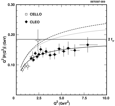
Figure 18: Comparison of the CLEO-results (points) for $Q^{2}F_{\pi\gamma}(Q^{2})$ with the theoretical predictions made by [206] using the asymptotic DA (solid curve) and the Chernyak-Zhitnitsky DA of Eq. (89) (dashed curve). The dotted curve shows the prediction made with the Chernyak-Zhitnitsky DA when its QCD evolution is taken into account. The solid line at $2f_{\pi}$ indicates the asymptotic value. Plot taken from [191].

In [219] the transition form factor $F_{\pi\gamma^{*}}(Q^{2},{Q^{\prime}}^{2})$ was calculated using a QCD sum rule for the three-point correlator associated with the process $\gamma^{*}\gamma^{*}\to\pi^{0}$, see Fig. 19 for the lowest-order perturbative diagrams contributing to it. Applying a factorization procedure to separate off the infrared singularities emerging in the limit ${Q^{\prime}}^{2}\to 0$, subsequently absorbing these singularities into bilocal correlation functions, and finally assuming certain forms for these correlation functions, the $Q^{2}$ dependence of the transition form factor $F_{\pi\gamma}(Q^{2})$ was studied and compared with the data from CELLO [192], see Fig. 20. As a result, again evidence was provided by this approach to $F_{\pi\gamma}(Q^{2})$ that $\bar{\varphi}(x,Q^{2})$ is rather close to the asymptotic form $\bar{\varphi}(x,Q^{2}\to\infty)=6x(1-x)$.

Figure 19: Lowest-order diagrams in perturbative QCD for the three-point correlator $2\pi i\int d^{4}xd^{4}y\,\mbox{e}^{-iqx}\mbox{e}^{ipx}\left\langle Tj^{5}_{\lambda}(y)j_{\mu}(x)j_{\nu}(0)\right\rangle$ where $j^{5}_{\lambda}=\bar{u}\gamma_{5}\gamma_{\lambda}u-\bar{d}\gamma_{5}\gamma_{\lambda}d$, and $j_{\mu}$ denotes the electromagnetic current, $j_{\mu}=\frac{2}{3}\bar{u}\gamma_{\mu}u-\frac{1}{3}\bar{d}\gamma_{\mu}d$. Taken from [219].

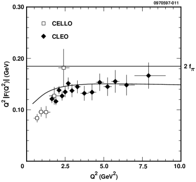
Figure 20: Comparison of the CLEO-results (points) for $Q^{2}F_{\pi\gamma}(Q^{2})$ with the prediction of [219] which is based on a QCD sum rule for $F_{\pi\gamma^{*}}(Q^{2}=-q^{2},{Q^{\prime}}^{2}=-{q^{\prime}}^{2})$ with two virtual photons. The limit ${Q^{\prime}}^{2}\to 0$ was taken after applying a factorization procedure for the infrared singularities which arise perturbatively in this limit. Taken from [191].

The same conclusion was reached in [220] where a light-cone sum rule (see next section for its foundations) for the two-point correlator

$$\int d^{4}x\,\mbox{e}^{-iqx}\,\left\langle\pi^{0}(p)|Tj_{\mu}(x)j_{\nu}(0)|0\right\rangle\$$ (102)

of the electromagnetic currents was used in the variable ${Q^{\prime}}^{2}$. In the chiral limit the light-cone OPE for the transition form factor $F_{\pi\gamma}(Q^{2})$ can then be written in terms of a dispersion integral over the imaginary part of the transition form factor $\mbox{Im}\,F_{\pi\gamma^{*}}(Q^{2},s)$ which, in turn, is given by the pion DA up to twist four as

$$\frac{1}{\pi}\mbox{Im}F_{\pi\gamma^{*}}(Q^{2},s)=\frac{\sqrt{2}f_{\pi}}{3}\left.\left(\frac{\bar{\varphi}_{\pi}(u,Q^{2})}{s+Q^{2}}-\frac{1}{Q^{2}}\frac{d\bar{\varphi}^{(4)}(u,Q^{2})}{ds}\right)\right|_{u=\frac{Q^{2}}{s+Q^{2}}}\,$$ (103)

where $\bar{\varphi}^{(4)}$ denotes the twist-four part. As a result, even at a higher order in twist the asymptotic DA is again favored by the CLEO and CELLO data, see Fig. 21. Notice, however, that a very recently performed analysis of the CLEO and CELLO data using a light-cone sum rule with the inclusion of twist four and $O(\alpha_{s})$ perturbative corrections to the pion DA seems to exclude both the asymptotic as well as the Chernyak-Zhitnitsky form of the DA at lowest twist [222, 221]. Still, in the determination of the pion DA from a nonlocal sum rule at the same order in twist and $\alpha_{s}$ a nonlocality parameter $\Lambda_{q}^{2}=0.4\,$GeV² is compatible with the result obtained from the light-cone sum rule. Seemingly, the inclusion of radiative corrections has a greater effect on the deviation from the asymptotic DA than the inclusion of the twist-four correction. This fits well with the result of [223] where the sum rule for the moments $\left\langle\xi^{N}\right\rangle$ with nonlocal condensates (including the $A_{1}$ resonance explicitly into the spectral function) and $O(\alpha_{s})$ corrections but no twist-four corrections was analyzed.

Figure 21: Comparison of $Q^{2}F_{\pi\gamma}(Q^{2})$ as obtained from the analysis using a light-cone sum rule [220] and the experimental data. The solid line is associated with the asymptotic DA, the long-dashed line with the Chernyak-Zhitnitsky DA, the dash-dotted line with the simple interpolation formula $F_{\pi\gamma}(Q^{2})=\frac{\sqrt{2}f_{\pi}}{4\pi^{2}f_{\pi}^{2}+Q^{2}}$ in [186], and the short-dashed line with a DA obtained in [188]. Plot taken from [220].

A number of calculations of the twist-two pion DA $\bar{\varphi}$ were recently performed using instanton models [225, 226] or in an instanton motivated model [227]. As compared to the asymptotic DA all of these investigations found a slight depletion of the model DA within the central region but no qualitative deviation from the asymptotic form.

We may thus conclude that the compatibility (noncompatibility) of the pion DA directly extracted from the experimentally well measured transition form factor $F_{\pi\gamma}(Q^{2})$ and the pion DA obtained from a sum rule involving a truncated, practical OPE with nonlocal (local) condensates provides rather strong phenomenological evidence that a local expansion of nonperturbative gauge invariant correlation functions is not sufficient to describe the hard and exclusive process $\gamma\gamma^{*}\to\pi^{0}$.

The technically more involved and theoretically more shaky case of $\rho$ meson DAs will not be discussed in detail in this review. We only mention here the QCD sum-rule analysis of Refs. [229, 205] using a truncated, practical OPE with local and nonlocal condensates $(\Lambda_{q}^{2}\sim 0.4$ GeV${}^{2})$, respectively. In both cases only leading twist was considered and, in contrast to the old calculation of Refs. [185, 233, 234], radiative corrections to the perturbative parts of the sum rules were taken into account. In [229] a sign error in the four-quark contribution to the OPE for the second moment of $\bar{\varphi}_{\perp}$ was pointed out leading to a drastic change in the prediction of the shape of this DA as compared to the prediction in [185, 233, 234]. A comparison between $\bar{\varphi}_{\parallel}$ at a normalization scale $\mu=1$ GeV, obtained from the sum rules for the zero-helicity state reveals no essential difference in both approaches. The treatment with nonlocal condensates, however, gives a much better stability of the Borel curves of the moments $\left\langle\xi^{N}\right\rangle$ up to large $N$ than it does in the local case where a large-$N$ prediction is unreliable, see Eq. (87) for a similar situation in the pion case. The shape of $\bar{\varphi}_{\parallel}$ obtained in [229, 205] is rather close to the result in [185, 233, 234] which is not too far from the asymptotic one; for $\bar{\varphi}_{\perp}$, however [229] get a much wider distribution than Chernyak and Zhitnitsky. Let us also mention that a computation of $\bar{\varphi}_{\perp}$ was performed in the framework QCD sum rules with nonlocal condensates in [224].

To summarize, we have seen that the use of nonlocal condensates in the OPEs of current correlators which determine the moments of mesonic DAs is superior to the treatment with local condensates in the following ways: (i) the prediction of high moments $\left\langle\xi^{N}\right\rangle$ is feasible, (ii) Borel sum rules for a given moment exhibit a wide window of stability, (iii) the prediction of close-to-asymptotic behavior of the lowest-twist pion DA using nonlocal condensates in spectral sum rules for the first few moments agrees well with an independent determination in terms of light-cone sum rules using the experimental data on the transition form factor $F_{\pi\gamma}(Q^{2})$ as a phenomenological input.

7.3 Reshuffling the OPE

Motivated by the phenomenological results in the last section we will in this section review the theoretical foundations for a light-cone expansion of a current-current correlator into gauge invariant, nonlocal operators. Taking the hadron-to-hadron (hadron-to-vacuum) matrix elements of this expansion allows to relate experimentally measurable deep inelastic scattering (transition) cross sections to structure functions (distribution amplitudes).

A phenomenological expansion of (2-point) nonlocal operator averages and Wilson coefficients into nonlocal objects, which captures more information about the nonlocal operator average than its truncated local expansion, is proposed for the vacuum-to-vacuum case. This approach introduces a so-called resolution parameter. The nonperturbative evolution of the nonlocal objects in this parameter will be derived. Several applications will be discussed, and a “running” gluon condensate will be extracted from experimental data in two channels. The implications of our nonlocal modification of the OPE in view of the nature of this expansion and an OPE-based realization of local quark-hadron duality are investigated phenomenologically.

7.3.1 Light-cone expansion into string operators of a current-current product

We have already mentioned in the last section the use of light-cone sum rules as a means to extract information on the twist-two pion DA from the experimental data for the transition form factor $F_{\pi\gamma}$ [220]. In this section we will give some theoretical background for this expansion.

The light-cone expansion of an object like $iTj_{\mu}(x)j_{\nu}(-x)$, $j_{\mu}$ being the electromagnetic current, into nonlocal string operators [240, 239, 236] and the know-how about the perturbative renormalization of the latter under a change of scale are of paramount importance for the experimental determination of hadronic structure functions (hadron-to-hadron matrix element of nonlocal operator) and DAs (hadron-to-vacuum matric element of nonlocal operator). Within perturbation theory the proof for the existence of the light-cone expansion of a current-current correlator in terms of quark twist-two string operators like

$$\bar{\psi}(x)\lambda^{a}\hat{x}{\cal P}\exp\left[ig\int_{0}^{x}dz^{\mu}\,A_{\mu}(z)\right]\psi(0)\equiv\bar{\psi}(x)\lambda^{a}\hat{x}[x,0]\psi(0)\,$$ (104)

was given in [235]. In Eq. (104) $\lambda^{a}$ is a flavor Gell-Mann matrix and $\hat{x}\equiv\gamma_{\mu}x^{\mu}$. Some time later the one-loop dependence of gauge-string operators on the renormalization scale $\mu$ was calculated in [236] by integrating over fluctuations $q^{q}$ and $A_{\mu}^{q}$ about classical backgrounds $q^{c}$ and $A_{\mu}^{c}$. The relevant diagrams are shown in Fig. 22.

Using the Fock-Schwinger gauge $x^{\mu}A^{c}_{\mu}=0$, the background gauge-string $[\alpha x,0]$ is unity and thus is omitted in some of the expressions to follow below. Evaluating the diagrams in Fig. 22 and keeping only the first logarithmic term in $x^{2}$, one then obtains [236]

$$\left.\bar{\psi}(x)\lambda^{a}\hat{x}\psi(0)\right|_{\mu_{2}^{2}}=\int_{0}^{1}d\alpha\int^{\alpha}_{0}d\beta\,\left[\delta(1-\alpha)\delta{\beta}-\frac{2\alpha_{s}}{3\pi}\log\frac{\mu_{2}^{2}}{\mu_{1}^{2}}\,K(\alpha,\beta)\right]\left.\bar{\psi}(\alpha x)\lambda^{a}\hat{x}\psi(\beta x)\right|_{\mu_{1}^{2}}\,$$ (105)

where

$$K(\alpha,\beta)=\frac{1}{2}\,\delta(1-\alpha)\delta({\beta})-\delta(\alpha)\left[\frac{1-\beta}{\beta}-\delta({\beta})\int d\beta^{\prime}\frac{1-\beta^{\prime}}{\beta^{\prime}}\right]-\delta(\beta)\left[\frac{\alpha}{1-\alpha}-\delta({\alpha})\int d\alpha^{\prime}\frac{\alpha^{\prime}}{1-\alpha^{\prime}}\right]-1\,.$$ (106)

The leading logarithms in Eq. (105) can be summed by solving a one-loop renormalization-group equation. In analogy to an expansion of a local operator into an eigenbasis (conformal operators, multiplicatively renormalized) of the evolution kernel one may also expand a nonlocal string operator into a nonlocal eigenbasis. The result is[236]

$$\left.\bar{\psi}\left(\frac{\alpha+\beta}{2}x\right)\lambda^{a}\hat{x}\left[\frac{\alpha+\beta}{2}x,\frac{\alpha-\beta}{2}x\right]\psi\left(\frac{\alpha-\beta}{2}x\right)\right|_{\mu_{2}^{2}}$$ (107)

$$= \int\frac{dk}{4\pi}\,\mbox{e}^{-ik\alpha}\int_{-1/2-i\infty}^{-1/2+i\infty}dj\,(j+\frac{1}{2})\,\beta^{-3/2}J_{j+1/2}(k\beta)\int_{-\infty}^{\infty}d\alpha^{\prime}\,\mbox{e}^{ik\alpha^{\prime}}\int_{0}^{\infty}d\beta^{\prime}\,\sqrt{\beta^{\prime}}H^{2}_{j+1/2}(k\beta^{\prime})\left(\frac{\alpha(\mu_{1}^{2})}{\alpha(\mu_{2}^{2})}\right)^{-\gamma_{j}}$$

$$\times\left.\bar{\psi}\left(\frac{\alpha^{\prime}+\beta^{\prime}}{2}x\right)\lambda^{a}\hat{x}\left[\frac{\alpha^{\prime}+\beta^{\prime}}{2}x,\frac{\alpha^{\prime}-\beta^{\prime}}{2}x\right]\psi\left(\frac{\alpha^{\prime}-\beta^{\prime}}{2}x\right)\right|_{\mu_{1}^{2}}\,$$

where $J_{j+1/2}(H_{j+1/2})$ is a Bessel(Hankel) function,

$$\gamma_{j}=\frac{8}{3b}\int_{0}^{1}du\,u^{j-1}\left[\frac{1}{2}\,\delta(1-u)-(1-u)-2\left(\frac{u}{1-u}-\delta(u)\int du^{\prime}\frac{u^{\prime}}{1-u^{\prime}}\right)\right]\,,$$ (108)

and the integrations over $\alpha^{\prime},\beta^{\prime}$ and $k,j$ indicate the projection onto and the (continuous) decomposition into renormalization-group covariant, conformal string operators, respectively.

Figure 22: Diagrams contributing to the one-loop renormalization of the flavor-nonsinglet string operator of Eq. (104). Thick lines denote the classical gauge string, crossed lines classical fermion fields and dashed lines are fluctuating gluon fields.

In addition to the quark string operators of Eq. (104) there is a twist-two flavor singlet gluon string operator which enters the light-cone expansion of a current-current correlator. It is given as

$$G(u,v)=x_{\alpha}G_{\mu\alpha}^{a}(ux)\,[ux,vx]_{ab}\,G_{\mu\beta}^{b}(vx)x_{\beta}\,$$ (109)

where the straight-path Wilson line $[ux,v,x]_{ab}$ is now in the adjoint representation! The flavor singlet quark string operator

$$\tilde{Q}(u,v)=\frac{i}{2}\left[\bar{\psi}(ux)\hat{x}[ux,vx]\psi(vx)-\bar{\psi}(vx)\hat{x}[vx,ux]\psi(ux)\right]$$ (110)

and the gluon string operator of Eq. (109) mix under renormalization, see Fig. (23).

Figure 23: Diagrams responsible for the mixing of twist-two, flavor singlet quark string operators and flavor singlet gluon string operators.

Formulas simular to the one in Eq. (107) relate $\tilde{Q}$ and $G$ at a renormalization point $\mu_{2}^{2}$ to a linear combination of their respective conformal expansions at some other renormalization point $\mu_{1}^{2}$, details can be found in [236]. The derivation for the evolution of string operators containing three Wilson lines is similar except for the fact that conformal symmetry is not sufficient to determine the solution explicitly.

It was shown in [236, 239] how the light-cone expansion of a $T$ product like $Tj_{\mu}(x)j_{\nu}(-x)$ into nonlocal string operators instead of local operators (in the latter case the choice of a suitable operator bases at a given nonleading twist is obscure because there are relations between the local operators dictated by the equations of motion [238, 237]) leads to a compact and much better managable series in singularities in deviations from the light-cone $x^{2}=0$ than in the local case. The leading term $-\frac{1}{16\pi^{2}x^{4}}\bar{\psi}(x)\gamma_{\mu}\hat{x}\gamma_{\nu}\bar{Q}^{2}\psi(-x)$, where $\bar{Q}=\frac{1}{2}\lambda^{3}+\frac{1}{2\sqrt{3}}\lambda^{8}$ is the charge matrix, has no definite twist. To project onto the leading twist, one can perform a symmetrization and trace subtraction in the local expansion of this string operator, which can be reassembled into a nonlocal expression. Higher twist contributions are technically quite involved.

The nonlocal light-cone expansion of [236] was used extensively in phenomenology. Besides the applications already addressed in the last section let us just mention two more examples: Light-cone sum rules were employed in [241] to predict the heavy-mesons couplings to pions in nonleptonic $D$ and $B$ decays in terms of two- and three- particle DAs up to twist four. The pion form factor at intermediate momentum $Q\sim 1\,$GeV was estimated in [242] using light-cone sum rules with higher twist distributions and radiative corrections.

7.3.2 Delocalized operator expansion

After having discussed the expansion of a $T$ product of electromagnetic currents into nonlocal string operators in view of applications involving a nonlocal hadron-to-vacuum matrix element or a nonlocal hadron-to-hadron matrix element we turn now to the case of a vacuum-to-vacuum average which leads to the occurrence of nonlocal condensates. The discussion of [73], which we follow, will be on a more phenomenological level. We have already introduced the approach of [197, 198, 199, 200, 205] to nonlocal condensates in Euclidean spacetime in Sec. 7.2.2.

Let us first discuss the case of two-point condensates. They are associated with nonlocal versions of the quark and gluon condesates in the conventional OPE. The parametrization of the nonlocal scalar quark condensate in Eq. (95) is to a good approximation also applicable to the nonlocal gluon condensate in Euclidean spacetime: In Fock-Schwinger gauge we have [200]

$$\left\langle A_{\mu}^{a}(z)A_{\nu}^{b}(y)\right\rangle=\delta^{ab}\left(y_{\mu}z_{\nu}-\delta_{\mu\nu}(z\cdot y)\right)\frac{\left\langle G^{2}\right\rangle}{384}\times g((z-y)^{2},z^{2},y^{2})+\cdots$$ (111)

where the local expansion of $g((z-y)^{2},z^{2},y^{2})$ reads

$$g((z-y)^{2},z^{2},y^{2})=1-\frac{\left\langle GD^{2}G\right\rangle-\frac{2}{3}\left\langle j^{2}\right\rangle}{18\left\langle G^{2}\right\rangle}\left((y-z)^{2}+\frac{y^{2}+z^{2}}{8}\right)+\cdots\approx g((z-y)^{2})\,.$$ (112)

In Eq. (111) the paranthesis denote contributions to $\left\langle A_{\mu}^{a}(z)A_{\nu}^{b}(y)\right\rangle$ which are not captured by the scalar function $g((z-y)^{2},z^{2},y^{2})$. Clearly, the dependence on $(y-z)^{2}$ is much stronger than the dependence on $y^{2}$ or $z^{2}$. The dependence on the latter two variables thus can be omitted on the level of accuracy at which the local condensates are known. In the expansion of the scalar part $T(q^{2})$ of a given current-current correlator $i\int d^{4}x\,\left\langle Tj_{\mu}(x)j_{\nu}(0)\right\rangle$ the Lorentz, color, and flavor indices in front of the nonlocal condensate get contracted and integrations over $x,y,$ and $z$ are performed. The nonperturbative correction to $T_{pert}(q^{2})$ arising from a two-point condensate $g(x^{2})$ can thus be written as

$$\int_{-\infty}^{\infty}d^{4}x\,f(x_{1},\ldots,x_{4})\,g(x^{2}) = \sum_{n_{1},\ldots,n_{4}=0}^{\infty}f_{n_{1},\ldots,n_{4}}(\Omega)\,g_{n_{1},\ldots,n_{4}}(\Omega)\,,\quad$$ (113)

where

$$f_{n_{1},\ldots,n_{4}}(\Omega) \equiv \int d^{4}x\,f(x_{1},\ldots,x_{4})\,\bigg{[}\,\prod_{i=1}^{4}\frac{H_{n_{i}}(\Omega x_{i})}{(2\,\Omega)^{n_{i}}}\,\bigg{]}$$ (114)

$$= \left.\bigg{[}\,\prod_{i=1}^{4}\,\frac{1}{(2\,\Omega)^{n_{i}}}\,H_{n_{i}}\bigg{(}\Omega\bigg{(}i\frac{d}{dk_{i}}\bigg{)}\bigg{)}\,\bigg{]}\,\tilde{f}(k_{i},\ldots,k_{4})\right|_{k_{1},\ldots,k_{4}=0}\,,$$

$$g_{n_{1},\ldots,n_{4}}(\Omega) \equiv \int d^{d}x\,\bigg{[}\,\prod_{i=1}^{4}\frac{\Omega^{n_{i}+1}}{\sqrt{\pi}\,n_{i}!}\,H_{n_{i}}(\Omega x_{i})\,\bigg{]}\,\mbox{e}^{-\Omega^{2}x^{2}}\,g(x_{1},\ldots,x_{4})$$ (115)

$$= \int\frac{d^{4}k}{(2\pi)^{4}}\,\bigg{[}\,\prod_{i=1}^{4}\,\frac{(ik_{n_{i}})^{n_{i}}}{n_{i}!}\,\bigg{]}\,\mbox{e}^{-\frac{k^{2}}{4\Omega^{2}}}\,\tilde{g}(k_{1},\ldots,k_{4})\,.$$

A number of comments are in order. In Eq. (113) the function $f(x_{1},\ldots,x_{4})$ denotes the strongly-peaked at $x=0$, perturbatively calculable, short-distance dependence as it arises in Euclidean spacetime after separating off the condensate part in an application of the background-field method. It corresponds to the Wilson coefficient for the local condensate in position space and has a width $\Delta_{f}$ which is comparable to the inverse external momentum $Q^{-1}$, see Fig. (24).

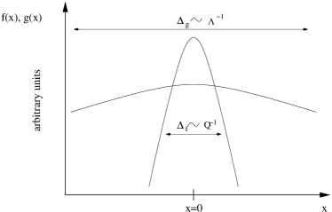
Figure 24: Schematic drawing of the short-distance function $f(x)$ and the 2-point condensate $g(x)$ illustrating the scale hierarchy $\Delta_{f}/\Delta_{g}\sim\Lambda/Q\ll 1$. Plot taken from [73].

To arrive at the second line a complete set of functions $e^{\Omega}_{n_{1}\cdots n_{4}}(x)$ and $\tilde{e}^{\Omega}_{n_{1}\cdots n_{4}}(x)$, which span a dual space with respect to the bilinear form

$$(f,g)\,\equiv\,\int d^{4}x\,f(x_{1},\cdots,x_{4})\,g(x^{2})\,$$ (116)

and which are normalized to

$$\left(\,e^{\Omega}_{n_{1},\cdots,n_{4}}\,,\,\tilde{e}^{\Omega}_{m_{1},\cdots,m_{4}}\,\right)\,=\,\delta_{n_{1}m_{1}}\cdots\delta_{n_{4}m_{4}}\,,$$ (117)

has been inserted inbetween $f$ and $g$. In the limit, where the resolution parameter $\Omega$ goes to infinity, $\Omega\to\infty$, the set $e^{\Omega}_{n_{1}\cdots n_{4}}(x)$ and $\tilde{e}^{\Omega}_{n_{1}\cdots n_{4}}(x)$ reproduces the local expansion of the nonlocal condensate, and we have

$$e^{\Omega\to\infty}_{n_{1}\cdots n_{4}}(x)\,\equiv\,\frac{(-1)^{n_{1}+\cdots+n_{4}}}{n_{1}!\cdots n_{4}!}\,\delta^{(n_{1})}(x_{1})\cdots\delta^{(n_{4})}(x_{4})\qquad\mbox{and}\qquad\tilde{e}^{\Omega\to\infty}_{n_{1}\cdots n_{4}}(x)\,\equiv\,x_{1}^{n_{1}}\cdots x_{4}^{n_{4}}\,.$$ (118)

In Eq. (118) $\delta^{(n_{i})}$ denotes the $n_{i}$th derivative of the delta function. For definiteness, we have chosen in Eqs. (114),(115) the following set of products of Hermite polynomials and their duals

$$e_{n_{1},\cdots,n_{4}}^{\Omega}(x) \equiv \frac{\Omega^{(n_{1}+1)+\cdots+(n_{4}+1)}}{\pi^{2}\,n_{1}!\cdots n_{4}!}\,H_{n_{1}}(\Omega x)\cdots H_{n_{4}}(\Omega x)\,\mbox{e}^{-\Omega^{2}(x_{1}^{2}+\cdots+x^{2}_{4})}\,,$$

$$\tilde{e}_{n_{1},\cdots,n_{4}}^{\Omega}(x) \equiv \frac{H_{n_{1}}(\Omega x)\cdots H_{n_{4}}(\Omega x)}{(2\,\Omega)^{n_{1}+\cdots+n_{4}}}\,.$$ (119)

Obviously, the basis (119) reduces to the basis (118) in the limit $\Omega\to\infty$. Different choices of one-parameter basis functions are equally well possible. Let us emphasize at this point that the delocalization of the OPE, which is achieved in this manner differs from [197, 198, 199, 200, 205] by the fact that with a truncation of the expansion (113) at $n_{1}=0,\cdots,n_{4}=0$ a resolution parameter, which eventually will be chosen to be equal to the applied external momentum, cuts off the irrelevant long-distance contribution of the nonlocal condensate $g(x^{2})$ to the integral. The Wilson coefficient in momentum space is equal to the one of the local expansion in this truncation, and this leads effectively to the running of the condensate with resolution. In Sec. 7.3.7 an alternative approach to running condensates will be discussed and applied.

The properties of Hermite polynomials dictate the following evolution equations for $f_{n_{1},\ldots,n_{4}}(\Omega)$ and $g_{n_{1},\ldots,n_{4}}(\Omega)$

$$\frac{d}{d\,\Omega}\,f_{n_{1},\ldots,n_{4}}(\Omega) = \frac{(n_{1}-1)\,n_{1}}{2\,\Omega^{3}}\,f_{n_{1}-2,\ldots,n_{4}}(\Omega)+\ldots+\frac{(n_{4}-1)\,n_{4}}{2\,\Omega^{3}}\,f_{n_{1},\ldots,n_{4}-2}(\Omega)\,,$$

$$\frac{d}{d\,\Omega}\,g_{n_{1},\ldots,n_{4}}(\Omega) = -\,\frac{(n_{1}+1)(n_{1}+2)}{2\,\Omega^{3}}\,g_{n_{1}+2,\ldots,n_{4}}(\Omega)-$$ (120)

$$\hskip 28.45274pt\ldots-\frac{(n_{4}+1)(n_{4}+2)}{2\,\Omega^{3}}\,g_{n_{1},\ldots,n_{4}+2}(\Omega)\,.$$

The parametric counting of the short-distance coefficients $f_{n_{1},\ldots,n_{4}}$ and the long-distance functions $g_{n_{1},\ldots,n_{4}}$ is similar as in the local expansion for $\Omega>Q$, the leading local terms are corrected by a finite sum over powers in $Q/\Omega$ in the former case and an infinite sum over powers of $\Lambda/\Omega$ in the latter case. Here $\Lambda$ denotes the mass scale associated with the fall-off of $g(x^{2})$ in Euclidean spacetime, for details see Sec. (7.3.3).

The consideration of 2-point condensates outlined above can be generalized to $(N>2)$-point condensates by an auxiliary increase to $N-1$ spacetime dimensions on which the functions $f$ and $g$ depend.

7.3.3 The gluonic field strength correlator and bilocal quark condensate on the lattice

Here we review what is known from lattice simulations about the gauge invariant, gluonic field strength correlator which bears information on the nonlocal gluon condensate of Eq. (111). Appealing to Poincaré, parity and time inversion invariance in Euclidean spacetime, the following parametrization was introduced in [243]:

$$g_{\mu\nu\kappa\lambda}(x) \equiv G^{a}_{\mu\nu}(x)\,[x,0]_{ab}\,G^{b}_{\kappa\lambda}(0)$$ (121)

$$= (\,\delta_{\mu\kappa}\delta_{\nu\lambda}-\delta_{\mu\lambda}\delta_{\nu\kappa}\,)\,\Big{[}\,D(x^{2})+D_{1}(x^{2})\,\Big{]}$$

$$+\,(\,x_{\mu}x_{\kappa}\delta_{\nu\lambda}-x_{\mu}x_{\lambda}\delta_{\nu\kappa}+x_{\nu}x_{\lambda}\delta_{\mu\kappa}-x_{\nu}x_{\kappa}\delta_{\mu\lambda}\,)\,\frac{\partial D_{1}(x^{2})}{\partial x^{2}}\,.$$

To separate perturbative from nonperturbative contributions the scalar functions $D$ and $D_{1}$ are usually [244, 247, 246] fitted as

$$D(x^{2}) = A_{g}\,\exp\bigg{(}\!-\frac{|x|}{\lambda_{g}}\bigg{)}+\frac{a_{g}}{|x|^{4}}\,\exp\bigg{(}\!-\frac{|x|}{\lambda_{g}}\bigg{)}\,,$$

$$D_{1}(x^{2}) = A_{1}\,\exp\bigg{(}\!-\frac{|x|}{\lambda_{g}}\bigg{)}+\frac{a_{1}}{|x|^{4}}\,\exp\bigg{(}\!-\frac{|x|}{\lambda_{g}}\bigg{)}\,.$$ (122)

The power-like behavior in Eqs. (122) at small $|x|$ is believed to catch most of the perturbative physics, although it is known that partially summed perturbation theory may generate less divergent renormalon contributions at $|x|=0$ as well, see Sec. (5). As we have seen, the coefficients of these contributions are ambiguous. We ignore this subtlety and assume that the purely exponential terms in Eqs. (122) exclusively carry the nonperturbative information. We also note that due to the cusp of the exponential ansatz in Eq. (122), derivatives of the nonperturbative part have nonlogarithmic UV singularities at $x=0$ that can only be defined in a nonperturbative UV regularization scheme. This is obviously in conflict with the well-tested idea that UV singularities, when treated in renormalization-group improved perturbation theory, lead to a logarithmic, anomalous scaling of averages over local operators. It does then make no sense to assume the exponential behavior of Eq. (122) down to arbitrarily small distances - after all the lattice resolution at which the field strength correlator is measured is finite, $a^{-1}\sim 2\,$GeV. We will re-address this concern in Secs. 7.3.4 and 7.3.7. We also would like to mention that in the framework of a nonrelativistic effective-field-theory formulation of QCD a decomposition of the correlator (121) into color magnetic and color electric correlations yields an electric correlation length, which is smaller than the magnetic, one as a result of lattice measurements [252, 250, 251]. See also [261] for a relation between the decay widths of heavy quarkonia on the one hand and electric and magnetic gluon correlators on the other hand.

In a recent unquenched lattice simulation [246] (see also Ref. [247]), where the gluon field strength correlator was measured with a resolution of $a^{-1}\approx(0.1\,\mbox{fm})^{-1}\approx 2$ GeV between $3$ and $8$ lattice spacings, it was found that

$$\frac{A_{g}}{A_{1}}\,\approx\,9\qquad\mbox{and}\qquad\lambda_{g}^{-1}\,\approx\,0.7\,\mbox{GeV}\,.$$ (123)

Notice that the inverse correlation length is somewhat larger than the typical hadronization scale $\Lambda_{\rm QCD}$. While the actual size of $A_{g}$ and $A_{1}$ depend quite strongly on whether quenched or unquenched simulations are carried out and also on the values for the light quark masses assumed, the ratio $A_{g}/A_{1}$ and the correlation length $\lambda_{g}$ were found to be quite stable [246]. The $D_{1}$ contribution can be neglected since $A_{g}\gg A_{1}$ (see Eq. (121)), and one may then write

$$g_{\mu\nu\kappa\lambda}^{\rm non-pert}(x)\,=\,\frac{1}{12}\,(\,\delta_{\mu\kappa}\delta_{\nu\lambda}-\delta_{\mu\lambda}\delta_{\nu\kappa}\,)\,.\,g(|x|)\,$$ (124)

This has the same tensor structure as the local condensate $g_{\mu\nu\kappa\lambda}^{\rm non-pert}(0)$. It is in agreement with the local expansion of $g_{\mu\nu\kappa\lambda}$ which reads [140]

$$-\left\langle g^{2}G^{a}_{\mu\nu}\partial_{\rho}\partial_{\rho}G^{a}_{\alpha\beta}\right\rangle = 8\,O^{-}\left(\delta_{\mu\beta}\delta_{\alpha\nu}-\delta_{\mu\alpha}\delta_{\nu\beta}\right)$$ (125)

$$+\,O^{-}\left(\delta_{\mu\beta}\delta_{\alpha\nu}+\delta_{\alpha\nu}\delta_{\mu\beta}-\delta_{\alpha\mu}\delta_{\nu\beta}-\delta_{\beta\nu}\delta_{\mu\alpha}\right)$$

$$+\,O^{+}\left(\delta_{\mu\beta}\delta_{\alpha\nu}+\delta_{\mu\beta}\delta_{\alpha\nu}-\delta_{\mu\alpha}\delta_{\nu\beta}-\delta_{\nu\beta}\delta_{\mu\alpha}\right)\,,$$

where

$$O^{\pm}\,\equiv\,\frac{1}{72}\left\langle g^{4}j^{a}_{\mu}j^{a}_{\mu}\right\rangle\pm\frac{1}{48}\left\langle g^{3}f_{abc}G^{a}_{\mu\nu}G^{b}_{\nu\lambda}G^{c}_{\lambda_{\mu}}\right\rangle\,,$$ (126)

and $j^{a}_{\mu}$ denotes a light flavor-singlet current. Using exact vacuum saturation for the four-quark operator, $\alpha_{s}(\mu=0.7\,\mbox{GeV})=0.7$, and the following instanton-calculus determined value of the condensate $\left\langle g^{3}f_{abc}G^{a}_{\mu\nu}G^{b}_{\nu\lambda}G^{c}_{\lambda\mu}\right\rangle=0.045$ GeV⁶, and $\langle\bar{q}q\rangle=-(0.24\,\,\mbox{GeV})^{3}$, it can be shown that the tensor structure belonging to the local condensate dominates the remainder in $\left\langle g^{2}G^{a}_{\mu\nu}\partial_{\rho}\partial_{\rho}G^{a}_{\mu\nu}\right\rangle$ by a factor of about nine [73].

In the case of the scalar, gauge invariant quark correlator the situation is similar [248]. For the longitudinal vector quark correlator defined as

$$-\frac{x^{\mu}}{|x|}\bar{q}(x)\gamma_{\mu}[x,0]q$$ (127)

an about ten times smaller correlation length as compared to the scalar case was obtained in [248] with a four-flavor simulation (staggered fermions) at a lattice resolution of $a^{-1}\sim 2\,$GeV.

7.3.4 Model calculation of the nonperturbative shift in the ground-state energy of heavy quarkonium

In this section we demonstrate in a model calculation for the nonperturbative shift of the ground-state ($n^{\,2s+1}L_{j}=1^{\,3}S_{1}$) energy $E^{np}$ of the heavy quarkonia, where the “exact” result can be calculated, in dependence on the heavy-quark mass $m$ how much better the delocalized operator expansion converges as compared to the local expansion [73]. Our investigation is not intended to represent a phenomenological study of non-perturbative effects in heavy quarkonium energy levels.

Among the early applications of the OPE in QCD was the analysis of nonperturbative effects in heavy quarkonium systems [253, 254, 255]. Heavy quarkonium systems are nonrelativistic quark-antiquark bound states for which the following hierarchy of the relevant physical scales $m$ (heavy quark mass), $mv$ (relative momentum), $mv^{2}$ (kinetic energy) and $\Lambda_{\rm QCD}$ holds:

$$m\,\gg\,mv\,\gg\,mv^{2}\,\gg\,\Lambda_{\rm QCD}\,.$$ (128)

The spatial size of the quarkonium system $\sim(mv)^{-1}$ is much smaller than the typical dynamical time scale $\sim(mv^{2})^{-1}$. In practice the last of the conditions in Eq. (128), which relates the vacuum correlation length with the quarkonium energy scale, is probably not satisfied for any known quarkonium state, not even for $\Upsilon$ mesons [181]. Only for top-antitop quark threshold production condition (128) may be a viable assumption [257].

We adopt the local version of the multipole expansion (OPE) for the expansion in the ratios of the scales $m$, $mv$ and $mv^{2}$. The resolution dependent expansion (DOE) is applied with respect to the ratio of the scales $mv^{2}$ and $\Lambda_{\rm QCD}$. The former expansion amounts to the usual treatment of the dominant perturbative dynamics by means of a nonrelativistic two-body Schrödinger equation. The interaction with the nonperturbative vacuum is accounted for by two insertions of the local $\mathbf{x}\mathbf{E}$ dipole operator, $\mathbf{E}$ being the chromoelectric field. [253] The chain of VEV’s of the two gluon operator with increasing numbers of covariant derivatives times powers of quark-antiquark octet propagators [253], i.e. the expansion in $\Lambda/mv^{2}$, is treated in the DOE.

At leading order in the local multipole expansion with respect to the scales $m$, $mv$, and $mv^{2}$ the expression for the nonperturbative corrections to the ground state energy reads

$$E^{np}\,=\,\int_{-\infty}^{\infty}\!dt\,f(t)\,g(t)\,,$$ (129)

where

$$f(t)\,=\,\frac{1}{36}\,\int\frac{dq_{0}}{2\pi}\,\mbox{e}^{iq_{0}(it)}\,\int\!d^{3}\mathbf{x}\int\!d^{3}\mathbf{y}\,\phi(x)\,(\mathbf{x}\mathbf{y})\,G_{O}\bigg{(}\mathbf{x},\mathbf{y},-\frac{k^{2}}{m}-q_{0}\bigg{)}\,\phi(y)\,,$$ (130)

with

$$G_{O}\bigg{(}\mathbf{x},\mathbf{y},-\frac{k^{2}}{m}\bigg{)} = \sum_{l=0}^{\infty}\,(2l+1)\,P_{l}\bigg{(}\frac{\mathbf{x}\mathbf{y}}{xy}\bigg{)}\,G_{l}\bigg{(}x,y,-\frac{k^{2}}{m}\bigg{)}\,,$$

$$G_{l}\bigg{(}x,y,-\frac{k^{2}}{m}\bigg{)} = \frac{mk}{2\pi}\,(2kx)^{l}\,(2ky)^{l}\,\mbox{e}^{-k(x+y)}\,\sum_{s=0}^{\infty}\,\frac{L_{s}^{2l+1}(2kx)\,L_{s}^{2l+1}(2ky)\,s!}{(s+l+1-\frac{m\,\alpha_{s}}{12\,k})\,(s+2l+1)!}\,,$$

$$\phi(x) = \frac{k^{3/2}}{\sqrt{\pi}}\,\mbox{e}^{-kx}\,,\qquad$$

$$k = \frac{2}{3}\,m\alpha_{s}$$ (131)

The term $G_{O}$ is the quark-antiquark octet Green-function [255], and $\phi$ denotes the ground state wave function of the quarkonium system. The functions $P_{n}$ and $L_{n}^{k}$ are Legendre and Laguerre polynomials, respectively. Since we neglect the spatial extension of the quarkonium system with respect to the interaction with the nonperturbative vacuum, the insertions of the $\mathbf{x}\mathbf{E}$ operator probe only the temporal correlations in the vacuum. This effectively renders the problem one-dimensional. Notice that $t$ is the Euclidean time.

Since the spatial extension of the quarkonium system is neglected and the average time between interactions with the vacuum is of the order of the inverse kinetic energy, the characteristic width of the function $f$ in Eq. (130) is of order $(mv^{2})^{-1}\sim(m\alpha_{s}^{2})^{-1}$. The values of the first few local multipole moments $f_{n}(\infty)$, which correspond to local Wilson coefficients, read

$$\begin{array}[]{ll}f_{0}(\infty)\,=\,1.6518\,\frac{m}{36\,k^{4}}\,,&f_{2}(\infty)\,=\,1.3130\,\frac{m^{3}}{36\,k^{8}}\,,\\[8.53581pt] f_{4}(\infty)\,=\,7.7570\,\frac{m^{5}}{36\,k^{12}}\,,&f_{6}(\infty)\,=\,130.492\,\frac{m^{7}}{36\,k^{16}}\,,\\[8.53581pt] f_{8}(\infty)\,=\,4474.1\,\frac{m^{9}}{36\,k^{20}}\,,&f_{10}(\infty)\,=\,262709.3\,\frac{m^{11}}{36\,k^{24}}\,,\ldots\,.\end{array}$$ (132)

The term $f_{0}(\infty)$ agrees with Ref. [254, 255] and $f_{2}(\infty)$ with Ref. [258]. The results for $f_{n>2}(\infty)$ are new.

We use a lattice-inspired model function $g(t)$ for the nonperturbative gluonic field strength correlator of the form

$$g(t) = 12\,A_{g}\,\exp\Big{(}-\sqrt{t^{2}+\lambda_{g}^{2}}/\lambda_{g}+1\Big{)}\,,$$

$$A_{g} = 0.04~{}\mbox{GeV}^{4}\,,\qquad\lambda_{g}^{-1}\,=\,0.7~{}\mbox{GeV}\,,$$ (133)

This model has an exponential large-time behavior according to Eq. (122) and a smooth behavior for small $t$. The local dimension four gluon condensate in this model is

$$\Big{\langle}\frac{\alpha_{s}}{\pi}\,G_{\mu\nu}^{a}G_{\mu\nu}^{a}\Big{\rangle}\,=\,\frac{6\,A_{g}}{\pi^{2}}\,=\,0.024\,\,\mbox{GeV}^{4}\,.$$ (134)

The exact form of the model for the nonperturbative gluonic field strength correlator is not important for our purposes as long as the derivatives of $g(t)$ at $t=0$ are well defined, see e.g. Refs. [181, 259] for different model choices. Tab. 1 shows the exact result in the model (133) and the first four terms of the DOE of $E^{np}$ for quark masses $m=5,25,45,90,175$ GeV and for $\Omega=\infty$ and $\Omega=k^{2}/m$. For each value of the quark mass the strong coupling has been fixed by the relation $\alpha_{s}=\alpha_{s}(k)$.

					$\Omega=\infty$		$\Omega=k^{2}/m$
$m$		$k^{2}/m$	$E^{np}$		$f_{n}g_{n}$	$\sum^{n}_{i=0}f_{i}g_{i}$	$f_{n}g_{n}$	$\sum^{n}_{i=0}f_{i}g_{i}$
(GeV)	$\alpha_{s}$	(MeV)	(MeV)	$n$	(MeV)	(MeV)	(MeV)	(MeV)
$5$	$0.39$	$0.338$	$24.8$	0	$38.6$	$38.6$	$24.2$	$24.2$
				2	$-65.7$	$-27.2$	$-3.9$	$20.3$
				4	$832.7$	$805.5$	$12.1$	$32.4$
				6	$-35048.0$	$-34242.4$	$-43.1$	$-10.8$
$25$	$0.23$	$0.588$	$12.6$	0	$16.0$	$16.0$	$12.8$	$12.8$
				2	$-9.0$	$7.0$	$-1.2$	$11.5$
				4	$37.8$	$44.8$	$2.6$	$14.1$
				6	$-526.6$	$-481.8$	$-6.7$	$7.4$
$45$	$0.19$	$0.722$	$4.9$	0	$5.9$	$5.9$	$5.0$	$5.0$
				2	$-2.2$	$3.7$	$-0.4$	$4.6$
				4	$6.1$	$9.8$	$0.7$	$5.3$
				6	$-56.4$	$-46.6$	$-1.4$	$3.8$
$90$	$0.17$	$1.156$	$1.05$	0	$1.15$	$1.15$	$1.07$	$1.07$
				2	$-0.17$	$0.98$	$-0.04$	$1.02$
				4	$0.18$	$1.16$	$0.04$	$1.07$
				6	$-0.65$	$0.51$	$-0.07$	$1.00$
$175$	$0.15$	$1.750$	$0.245$	0	$0.258$	$0.258$	$0.249$	$0.249$
				2	$-0.016$	$0.242$	$-0.005$	$0.244$
				4	$0.008$	$0.250$	$0.003$	$0.247$
				6	$-0.012$	$0.237$	$-0.003$	$0.244$

Table 1: Nonperturbative corrections $E_{np}$ to the heavy quarkonium ground state level at leading order in the multipole expansion with respect to the scales $m$, $mv$ and $mv^{2}$ for various quark masses $m$ based on the model in Eq. (133). Displayed are the exact result and the first few orders in the DOE for $\Omega=\infty$ and $\Omega=k^{2}/m$. The numbers are rounded off to units of $0.1$, $0.01$ or $0.001$ MeV.

Notice that the series all appear to be asymptotic, i.e.  they are not convergent for any resolution. The local expansion ($\Omega=\infty$) is badly behaved for small quark masses because for $k^{2}/m<\lambda_{g}^{-1}$ any local expansion is meaningless. In particular, for $m=5$ GeV the subleading dimension-six term is already larger than the parametrically leading dimension-four term. For quark masses, where $k^{2}/m\geq\lambda_{g}^{-1}$, the local expansion is reasonably good. However, at the finite resolution $\Omega=k^{2}/m$, the size of higher order terms is considerably smaller than in the local expansion for all quark masses, and the series is apparently much better behaved. The size of the order-$n$ term is suppressed by approximately a factor $2^{-n}$ as compared to the order-$n$ term in the local expansion. We see explicitly that terms in the series with larger $n$ increase more quickly in magnitude in the local expansion scale as compared to expansion at finite resolution. One also observes that even in the case $k^{2}/m<\lambda_{g}^{-1}$, where the leading term of the local expansion overestimates the exact result, the leading term in the delocalized expansion for $\Omega=k^{2}/m$ agrees with the exact result within a few percent.

For a realistic treatment of the nonperturbative contributions in the heavy quarkonium spectrum a model-independent analysis should be carried out. In addition, also higher orders in the local multipole expansion with respect to the ratios of scales $m$, $mv$ and $mv^{2}$ should be taken into account, which have been neglected here. These corrections might be substantial, in particular for smaller quark masses.

7.3.5 Running gluon condensate from the $\bar{c}c$ spectrum

In this section we review an extraction of the running gluon condensate from the charmonium spectrum using moment sum rules [73]. We have already discussed this approach in Sec. (4.2) where an OPE was assumed (for an analysis involving operators at $n=8$ see [72]. The $n$th moment ${\cal M}_{n}$ reads [140]

$${\cal M}_{n} = \frac{3}{4\pi^{2}}\frac{2^{n}(n+1)(n-1)!}{(2n+3)!!}\,\frac{1}{(4m_{c}^{2})^{n}}\,\bigg{\{}\,1\,+\,\mbox{[pert. corrections]}$$

$$\hskip 28.45274pt\,+\,\delta^{(4)}_{n}\,\langle g^{2}G^{2}\rangle\,+\,\Big{[}\,\delta^{(6)}_{G,n}\,\langle g^{3}fG^{3}\rangle\,+\,\delta^{(6)}_{j,n}\,\langle g^{4}j^{2}\rangle\,\Big{]}\,+\,\ldots\,\bigg{\}}\,,$$

where

$$\delta^{(4)}_{n} = -\frac{(n+3)!}{(n-1)!\,(2n+5)}\,\frac{1}{9\,(4m_{c}^{2})^{2}}\,,$$

$$\delta^{(6)}_{G,n} = \frac{2}{45}\frac{(n+4)!\,(3n^{2}+8n-5)}{(n-1)!\,(2n+5)\,(2n+7)}\,\frac{1}{9\,(4m_{c}^{2})^{3}}\,,$$

$$\delta^{(6)}_{j,n} = -\frac{8}{135}\,\frac{(n+2)!\,(n+4)\,(3n^{3}+47n^{2}+244n+405)}{(n-1)!\,(2n+5)\,(2n+7)}\,\frac{1}{9\,(4m_{c}^{2})^{3}}\,,$$ (135)

and $\langle g^{3}fG^{3}\rangle\equiv\langle g^{3}f^{abc}G^{a}_{\mu\nu}G^{b}_{\nu\lambda}G^{c}_{\lambda\mu}\rangle=0.045\,\,\mbox{GeV}^{6}$ (instanton gas approximation [21]), $\langle g^{4}j^{2}\rangle\equiv\langle g^{4}j^{a}_{\mu}j^{a}_{\mu}\rangle=-\rho\,4/3(4\pi)^{2}\alpha_{s}^{2}\langle\bar{q}q\rangle^{2}$ ($\alpha_{s}(\mu=0.7\,\mbox{GeV})=0.7$ and $\langle\bar{q}q\rangle=-(0.24\,\,\mbox{GeV})^{3}$, $\rho=1$ $\rightarrow$ exact vacuum saturation), $j^{a}_{\mu}$ being the light flavor singlet current. We work with the ratio

$$r_{n}\,\equiv\,\frac{{\cal M}_{n}}{{\cal M}_{n-1}}\,.$$ (136)

The extraction of the running of the gluon condensate is reliable provided that subleading, dimension-six power corrections in Eq. (135) are much smaller than the dimension-six power correction

$$\frac{1}{4\Omega^{2}}\,\delta^{(4)}_{n}\,\langle g^{2}GD^{2}G\rangle$$ (137)

stemming from the local expansion of the dimension-four running gluon condensate. Table 2 shows that in the OPE for $r_{n}$ this is indeed the case provided that $n$ is sufficiently large (in practice $n\geq 4$). As expected, Table 2 indicates that for a value of the four-quark condensate twice the value obtained from exact vacuum saturation the convergence of the dimension-six part of the running gluon condensate towards that of the full OPE is slower than in the case of exact vacuum saturation.

$n$	1	2	3	4	5	6	7	8
$\rho=1$	0.13	0.36	0.56	0.73	0.87	0.99	1.08	1.16
$\rho=2$	0.09	0.25	0.42	0.57	0.69	0.80	0.89	0.97

Table 2: Ratio of the local dimension-six contributions contained in the running gluon condensate and in the full OPE for $r_{n}$ as a function of $n$.

On the experimental side of the sum rules we have used the spectrum as compiled in [69], see this reference for details. To compare the running gluon condensate as extracted from the data with the model expression (using the lattice fit of Eq. (122) and the $n_{i}=0$ expression in Eq. (115)) we have to make a choice for the resolution scale $\Omega$. The following physical arguments apply: For large $n$, i.e.  in the nonrelativistic regime, the width of the short-distance function $f$ is of the order of the quark c.m. kinetic energy $mv^{2}$, which scales like $m/n$ because the average quark velocity in the $n$-th moment scales like $1/\sqrt{n}$ [260]. For small $n$, on the other hand, the relevant short-distance scale is just the quark mass. We take this as a guideline to use $\Omega=2m_{c}/n$ as the relevant resolution scale in the model expression

$$\Big{\langle}\frac{\alpha_{s}}{\pi}G^{2}\Big{\rangle}_{\rm lat}(\Omega)\,=\,\frac{6\,A_{g}}{\pi^{2}}\,\bigg{\{}\,1\,+\,\frac{1}{4\,\Omega^{2}\,\lambda_{g}^{2}}$$ (138)

$$\qquad-\,\frac{3\,\sqrt{\pi}}{4\,\Omega\,\lambda_{g}}\,\bigg{(}1+\frac{1}{6\,\Omega^{2}\,\lambda_{g}^{2}}\bigg{)}\,\mbox{e}^{1/(4\,\Omega^{2}\,\lambda_{g}^{2})}\,\bigg{(}\,1-{\rm erf}\Big{(}\frac{1}{2\,\Omega\,\lambda_{g}}\Big{)}\,\bigg{)}\,\bigg{\}}\,.\qquad$$

for the running gluon condensate ($\lambda_{g}^{-1}=0.7$ GeV and $A_{g}=0.04$ which corresponds to $\langle(\alpha_{s}/\pi)G^{2}\rangle_{\rm lat}(\infty)=0.024\,\,\mbox{GeV}^{4}$). In Fig. (25) the results of the data extraction and the model calculation are shown.

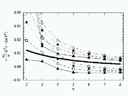
Figure 25: The running gluon condensate as a function of $n$ when extracted from the ratio of moments $r_{n}$ for $\overline{\mbox{MS}}$ charm-quark masses $\overline{m}_{c}(\overline{m}_{c})=1.23$ (white triangles), $1.24$ (black stars), $1.25$ (white squares) and $1.26$ GeV (black triangles). The area between the upper and lower symbols represents the uncertainties. The thick solid line indicates the running gluon condensate as it is obtained from the lattice-fitted ansatz in Eqs. (122). Plot taken from [73].

The $n$-dependence of the lattice-inspired running gluon condensate and the result obtained from the charmonium moment sum rules are consistent for larger $n$. For small $n$ no conclusive statement can be made, recall Table 2 and the fact that for small $n$ the sensitivity to the error in the continuum region of the spectrum is enhanced.

7.3.6 Running gluon condensate from the $\tau$ decay spectrum

In this section we review an independent extraction of the running gluon condensate from the spectral function of the $V+A$ channel [73] as it was measured in $\tau$ decays by Aleph [179] and Opal [180] at LEP. In this channel the OPE of the associated current-current correlator $i\int d^{4}\!x\,\mbox{e}^{iqx}\left\langle Tj_{\mu}^{L}(x)j_{\nu}^{R}(0)\right\rangle$ (with currents $j_{\mu}^{L/R}=\bar{u}\gamma_{\mu}(1\pm\gamma_{5})d$) is dominated by the gluon condensate [176, 177, 178], the dimension-six power corrections that are not due to the local expansion of the running gluon condensate are suppressed. We use a sum rule for the cutoff independent Adler function

$$D(Q^{2})\,\equiv\,-Q^{2}\,\frac{\partial\,\Pi^{\rm V+A}(Q^{2})}{\partial\,Q^{2}}\,=\,\frac{Q^{2}}{\pi}\,\int_{0}^{\infty}ds\,\frac{\mbox{Im}\,\Pi^{\rm V+A}(s)}{(s+Q^{2})^{2}}\,.$$ (139)

For the $V+A$ spectral function we have used the Aleph measurement [179] in the resonance region up to $2.2$ GeV². For the continuum region above $2.2$ GeV² 3-loop perturbation theory, which we also used on the OPE side, was employed (with $\alpha_{s}(M_{Z})=0.118$), and we have set the renormalization scale $\mu$ equal to $Q$. The Wilson coefficient for $\Big{\langle}\frac{\alpha_{s}}{\pi}G^{2}\Big{\rangle}$ was taken into account up to order $\alpha_{s}$ [131]. It can be read off from

$$T^{\rm V+A}_{\rm np}(Q^{2})\,=\,\frac{1}{6\,Q^{4}}\,\bigg{(}\,1-\frac{11}{18}\frac{\alpha_{s}}{\pi}\,\bigg{)}\,\Big{\langle}\frac{\alpha_{s}}{\pi}G^{2}\Big{\rangle}\,+\,\ldots\,.$$ (140)

With the same values for the local condensates as in Sec. 7.3.5 the evaluation of the dimension-six contribution in the OPE and the dimension-six contribution of the local expansion of the running gluon condensate yields a comparable magnitude and equal signs which gave us a phenomenological justification for the extraction of the running gluon condensate in the $V+A$ channel. Fig. 26 shows the result.

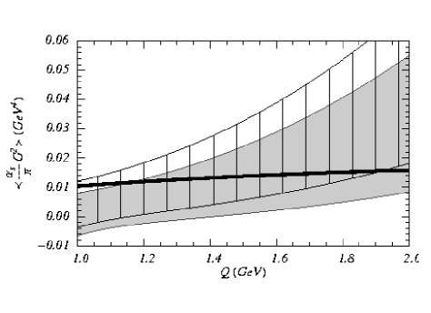
Figure 26: The running gluon condensate as a function of $Q$ when extracted from the Adler function. The grey area represents the allowed region using perturbation theory at ${\cal O}(\alpha_{s}^{3})$ and the striped region using perturbation theory at ${\cal O}(\alpha_{s}^{2})$. The thick solid line denotes the running gluon condensate as obtained from the lattice-fitted ansatz in Eqs. (122) for $\Omega=Q$. Plot taken from [73].

The uncertainties are due to the experimental errors in the spectral function and a variation of the renormalization scale $\mu$ in the range $Q\pm 0.25$ GeV. The analysis is restricted to the range $1\,\mbox{GeV}\leq Q\leq 2\,\mbox{GeV}$ because for $Q<1$ GeV perturbation theory becomes unreliable and for $Q>2$ GeV the experimentally unknown part of the spectral function at $s\geq 2.2$ GeV² is being probed. The thick black line in Fig. 26 shows the lattice-inspired model for the running gluon condensate of Eq. (138) for $\Omega=Q$. It is consistent with the phenomenological extraction and an increasing function of $Q$. Since the $Q$ dependence of the model is rather weak for $1\,\mbox{GeV}\leq Q\leq 2\,\mbox{GeV}$ and the error band of the extraction rather large it is not possible to draw a more quantitative conclusion at present.

7.3.7 Euclidean position-space $V\pm A$ correlators at short distance

In Sec. 7.3.2 a delocalized version of the OPE was obtained by projections of a perturbatively calculable short-distance function $f(x)$ and a nonperturbative, long-distance function $g(x^{2})$ on a resolution dependently “rotated” basis in dual space, see Eq. (113). Thereby, the function $g(x^{2})$ is assumed to be determined at infinite resolution. However, the only so-far available first-principle approach to $g(x^{2})$ is a lattice calculation which can only be performed at a finite resolution, $\Omega\sim a^{-1}$.

An alternative approach to running condensates than the one in Sec. 7.3.2 is to view the OPE as the usual local expansion but now involving averages over local composite operators at a resolution $\Omega\sim Q$. These operator averages are, besides their usual perturbative evolution, nonperturbatively coarse-grained in a gauge invariant way [145]. In the case of a composite with two fundamental operators like the quark or the gluon condensate nonperturbative coarse graining is performed by integrating out length scales between $\Omega^{-1}$ and $(\Omega-d\Omega)^{-1}$, which are associated with a loss in resolution of $\Omega^{2}/d\Omega$, in an $\Omega$ dependent, gauge invariant and nonperturbative correlation function $g(x,\Omega)$, using a sharply cut off spherical well

$$\frac{2\,(d\Omega)^{4}}{\pi^{2}}\,\theta\left(1/d\Omega-|x|\right)\,$$ (141)

as a weight function. If we assume self-similarity of $g(x,\Omega)$, that is, an exponential form

$$g(x,\Omega)=A(\Omega)\exp[-|x|/\lambda_{g}]\,,$$ (142)

where only the coefficient $A(\Omega)$ depends on $\Omega$, then the following evolution equation for $A(\Omega)$ is easily derived [145]

$$\frac{\partial}{\partial\Omega}A(\Omega)=\frac{4}{5\lambda}\Omega^{-2}A(\Omega)\,.$$ (143)

The solution of Eq. (143) corresponding to the running gluon condensate would then take the form

$$\langle\frac{\alpha_{s}}{\pi}G^{2}\Big{\rangle}(\Omega)=\frac{6A_{g}}{\pi^{2}}\exp\left[-\frac{4}{5\lambda_{g}}\left(\frac{1}{\Omega}-\frac{1}{\Omega_{lat}}\right)\right]\ .$$ (144)

when the lattice fit of Eq. (122) is used as a model with $\Omega_{lat}=a^{-1}=2\,$GeV.

Following [147] we now use dependences like Eq. (141) to investigate the effect of running condensates on the $|x|$ dependence of the Euclidean $V\pm A$ position-space correlators when they are expanded into a DOE in the chiral limit [121]

$$R_{V-A}(|x|\sim 1/\Omega) \equiv \frac{T^{V}(|x|)-T^{A}(|x|)}{2T_{0}(|x|)}=\frac{\pi^{3}}{9}\,\alpha_{s}(\Omega)\left\langle\bar{q}q\right\rangle_{\Omega}^{2}\,\log[(|x|\Omega)^{2}]\,|x|^{6}\,;$$

$$R_{V+A}(|x|\sim 1/\Omega) \equiv \frac{T^{V}(|x|)+T^{A}(|x|)}{2T_{0}(|x|)}=1-\frac{\pi^{2}}{96}\left\langle\frac{\alpha_{s}}{\pi}(F_{\mu\nu}^{a})^{2}\right\rangle_{\Omega}|x|^{4}-$$ (145)

$$\frac{2\pi^{3}}{81}\,\alpha_{s}(\Omega)\left\langle\bar{q}q\right\rangle_{\Omega}^{2}\,\log[(|x|\Omega)^{2}]\,|x|^{6}\,$$

in the $V\pm A$ channel. There is no perturbative and gluon-condensate contribution in $R_{V-A}$, the correlator is extremely sensitive to chiral symmetry breaking. For the treatment of the four-point quark correlators at $D=6$ we assume a factorization into scalar two-point quark correlators. In analogy to the case of the field strength correlator a lattice measurement of the scalar two-point quark correlator [248] with $N_{F}=4$ staggered fermions and a quark mass $am=0.01$ at $a^{-1}\sim 2\,$GeV yields

$$\lambda_{q}=3.1\,\mbox{GeV}^{-1}\ ,\ \ \ \ A_{q}(a^{-1}=\Omega_{lat}\sim 2\,\mbox{GeV})=(0.212\,\mbox{GeV})^{3}\,.$$ (146)

Substituting $\Omega=1/|x|$ in Eq. (7.3.7) and working with the parameters of Eqs.  (146), (133), and a fixed value of $\alpha_{s}(\Omega_{lat})=0.2$ [249], an $|x|$ dependence as depicted in Fig.  27 is obtained.

Figure 27: $R_{V\pm A}$ as a function of distance $x$ in the chiral limit. The solid line corresponds to the DOE with an assumed factorization of four-point quark correlators at $D=6$ into two-point, scalar quark correlators, the dashed line to the OPE. Crosses depict the result of the instanton liquid calculation of [126] which is taken from [121]. Plot taken from [147].

In addition to a much better agreement (in comparison to the OPE) with the result obtained in the instanton liquid [126] the result of the DOE calculation almost perfectly agrees with the result of a quenched lattice calculation obtained using an overlap action [121]. The result of an extraction of $R_{V\pm A}(|x|)$ from the $\tau$-decay data, see for example [126], slightly overshoots the DOE and lattice results which were obtained in the chiral limit see Fig. 28.

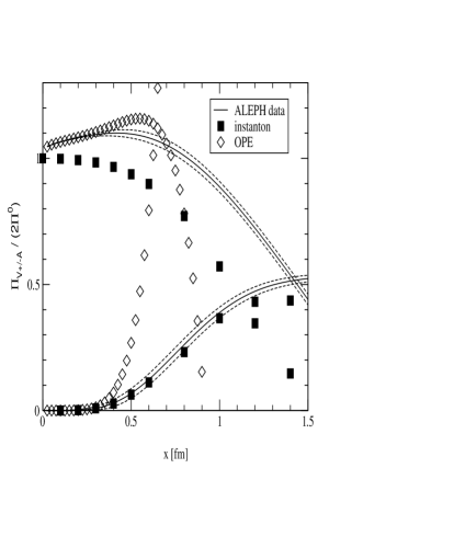
Figure 28: $R_{V\pm A}$ as a function of distance $x$. The dashed lines indicate the errors in the experimental determination of the respective spectral functions by Aleph. The squares show the results obtained in the model of a random instanton liquid. The diamonds are the OPE prediction using realistic light-quark masses. Plot taken from [126].

7.3.8 Mesonic spectra from the DOE?

The good agreement that we have found in Sec. 7.3.7 between Euclidean $V\pm A$ correlators when expanded into an OPE with running condensates and when computed on a lattice lead us to investigate to what extent one can predict properties of the spectral functions of light-quark channels within the resonance region from the (practical) OPE with running condensates by analytical continuation to time-like momenta, $Q^{2}=-(s+i\varepsilon)$ or $Q=-i\sqrt{s}$, $(s>0)$, and by taking the imaginary part afterwards [146]. For a contribution of the form

$$\frac{A_{4}(\Omega_{lat})}{(Q^{2})^{2}}\,\exp\left[-\frac{4}{5\lambda_{4}}\left(\frac{1}{Q}-\frac{1}{\Omega_{lat}}\right)\right]\,$$ (147)

the associated contribution to the spectral function reads

$$\frac{A_{4}(\Omega_{lat})}{s^{2}}\exp\left[\frac{4}{5\lambda_{4}}\frac{1}{\Omega_{lat}}\right]\sin\left[-\frac{4}{5\lambda_{4}\sqrt{s}}\right]$$ (148)

Notice that oscillations only start if $\sqrt{s}$ becomes smaller than the inverse correlation length $\lambda_{4}^{-1}$. As in Sec. 7.3.7 a factorization of four-quark correlators into scalar two-quark correlators within the usual vacuum saturation hypothesis of the local case is assumed. All running condensates thus have the form as in Eq. (148), the effective correlation length for running condensates of $D=6$ is $\lambda_{q}/2$.

Figure 29: The spectral functions $\mbox{Im}\Pi(Q^{2}=-s-i\varepsilon)$, $(s>0)$ for sets $(A)$ and $(B)$, where $(i)$, $(ii)$, $(iii)$, and $(iv)$ correspond to the $\rho$, $a_{1}$, $\pi$, and $\phi$ channels, respectively. The unit of $s$ is (GeV)². Taken from [146].

The $\rho$, $a_{1}$, $\pi$, and $\phi$ meson channels where investigated in [146], and the following two sets of parameters were used:

$$\underline{\mbox{Set}\,A:}$$

$$\lambda_{q} = 3.1\,\mbox{GeV}^{-1}\ ,\ \ \ \ A_{q}(a^{-1}=\Omega_{lat}\sim 2\,\mbox{GeV})=(0.212\,\mbox{GeV})^{3}\,,$$

$$\lambda_{g} = 1.7\,\mbox{GeV}^{-1}\ ,\ \ \ \ A_{g}(a^{-1}=\Omega_{lat}\sim 2\,\mbox{GeV})=0.015\,(\mbox{GeV})^{4}\,$$

$$\underline{\mbox{Set}\,B:}$$

$$\lambda_{q} = 0.3\,\mbox{GeV}^{-1}\ ,\ \ \ \ A_{q}(a^{-1}=\Omega_{lat}\sim 2\,\mbox{GeV})=(0.212\,\mbox{GeV})^{3}\,,$$

$$\lambda_{g} = 1.7\,\mbox{GeV}^{-1}\ ,\ \ \ \ A_{g}(a^{-1}=\Omega_{lat}\sim 2\,\mbox{GeV})=0.015\,(\mbox{GeV})^{4}\,.$$ (149)

The quark correlation length $\lambda_{q}$ in Set A corresponds to that of the scalar quark correlator, the one in Set B to the longitudinal vector quark correlator as obtained in [248]. Judging from Fig. 29, the result obtained with the small fermionic correlation length in Set B is more realistic but still far off the experimentally observed behavior. The most disturbing feature of the spectra in Fig. 29 is the fact that they become negative at low values of $s$. For a discussion of the moments of the spectra in Fig. 29 see [146]. This is unacceptable and certainly has to do with the incompleteness and hence poor practical convergence of the expansion at low momenta.

7.3.9 Speculations on convergence properties of expansions with nonperturbatively running operators

How does the partial resummation of operators involving powers of covariant derivatives, which leads to the nonperturbative running of the condensates in the usual OPE, possibly affect the “convergence” properties of the modified operator expansion? Let us give some (admittedly speculative) arguments.

First of all, one notices the difference between the exponential(-like) dependences of Eq. (144) (or Eq. (138)) with the situation in the instanton model in Sec. 6.2 where exponentially small terms of the form $\exp[\frac{Q}{\Lambda_{QCD}}]$ were observed. As it was argued in [142] the latter exponentials may occur in the exact result to cure the ambiguities of the $1/Q^{2}$ expansion which may arise due to the factorially-in-$D$ rising coefficients where $D$ roughly refers to the power in $1/Q$. A possibility is that this factorial divergence of coefficients would already be present in a modification $\overline{\mbox{OPE}}$ of the OPE where operators containing powers of covariant derivatives are omitted – the factorially-in-$D$ rising coefficients would then simply arise from the combinatorial variety of composites involving powers of quark and gluon field operators. So already the $\overline{\mbox{OPE}}$ and, more generally, each subseries of the OPE with a given, fixed power of covariant derivatives would be an asymptotic expansion which could be made unambiguous by adding exponentially small terms of the form $\exp[\frac{Q}{\Lambda_{QCD}}]$.

Second, in the OPE we may resum a part of the powers-of-covariant-derivative series associated with each operator in $\overline{\mbox{OPE}}$ by applying our methods of Secs. 7.3.2 or 7.3.7. For an operator of dimension $D$ the associated contribution after partial resummation is roughly of the form

$$\frac{A_{n}(\Omega_{lat})}{Q^{n}}\,\exp\left[-\lambda^{-1}_{n}\left(\frac{1}{Q}-\frac{1}{\Omega_{lat}}\right)\right]\,$$ (150)

where $\lambda_{n}$ denotes an effective correlation length. The expression in Eq.(150) has a maximum at $Q=(n\,\lambda_{n})^{-1}$ with value

$$P_{n}\equiv\left(\Lambda_{n}\,\lambda_{n}\,\exp[-1]\,n\right)^{n}\,\exp\left[\frac{\lambda^{-1}_{n}}{\Omega_{lat}}\right]\,$$ (151)

where $\Lambda_{n}\equiv(A_{n}(\Omega_{lat}))^{(1/n)}$. As can be motivated from the example of factorizing the four-quark correlations into two-quark correlations in Sec. 7.3.7 it is likely that $\lambda_{n}$ is a decreasing function of $n$. If we assume a fall-off as $\lambda_{n}=\lambda/n^{(1-\varepsilon)}$, $(1>\varepsilon>0)$ then the position of the maximum of the expression in Eq.(150) decreases as $Q_{n}=\lambda^{-1}n^{-\varepsilon}$. The value of the maximum in this case is

$$P_{n}=\left(\Lambda_{n}\,\lambda\,n^{\varepsilon}\,\exp[-1+\frac{n^{-\varepsilon}}{\lambda\Omega_{lat}}]\right)^{n}\,.$$ (152)

Assuming that $\Lambda_{n}$ does not depend on $n$, $\Lambda_{n}\equiv\Lambda_{QCD}$, as suggested by the phenomenology of practical OPEs, the critical mass dimension $n_{c}$ from which on maxima explode is given in implicit form as

$$\Lambda_{QCD}\,\lambda\,n_{c}^{\varepsilon}\,\exp[-1+\frac{n_{c}^{-\varepsilon}}{\lambda\Omega_{lat}}]=1\,.$$ (153)

A truncation of the OPE with running condensates at some $n<n_{c}$ would mean that physics below the maximum $Q_{n}$ can not be described, a truncation at $n\geq n_{c}$ does not make sense since due to the rapid increase of maxima at $n\geq n_{c}$ the expansion does not approximate anymore. Provided our above assumptions are met, another source of asymptotic behavior is identified. Let us give some numerical examples. For $\varepsilon=0.5$ and $\Lambda_{QCD}=0.4$ GeV (the rounded) value of $n_{c}$ was calculated as a function of $\lambda$ in [146] as

$$\lambda = 3\,\mbox{GeV}^{-1}\ \ \rightarrow\ \ n_{c}=4\ ;\ \ \ \ \ \ \,\lambda=2\,\mbox{GeV}^{-1}\ \ \ \ \ \rightarrow\ \ \ n_{c}=10\ ;$$

$$\lambda = 1\,\mbox{GeV}^{-1}\ \ \rightarrow\ \ n_{c}=40\ ;\ \ \ \ \ \lambda=0.5\,\mbox{GeV}^{-1}\ \ \ \rightarrow\ \ \ n_{c}=158\,.$$ (154)

In conclusion, we have argued that exponential-like behavior of the form

$$\exp[\frac{Q}{\Lambda_{QCD}}]\ \ \ \ \mbox{and}\ \ \ \ \exp\left[-\lambda^{-1}_{n}\left(\frac{1}{Q}-\frac{1}{\Omega_{lat}}\right)\right]$$ (155)

may coexist in an improved version of the OPE. The former may assure the uniqueness of the asymptotic $1/Q$ expansion involving operators with a given, fixed number of covariant derivatives [142] while the latter arises from a partial summation of the expansion in powers of covariant derivatives acting on a given, fixed composition of powers of quark and gluon operators.

8 Summary

In this article we have presented a review of theoretical approaches to the indentification of the mechanisms leading to the violation of local quark-hadron duality in QCD. We have started our discussion with a mini-review on QCD sum rules in (axial)vector-meson channels in vacuum, at finite temperature, and at finite baryon density. The status of renormalon singularities as possible sources for power corrections in the OPE was very briefly addressed. We then have reviewed two theoretical model approaches to the calculation of current correlators: the instanton-gas model and the ’t Hooft model. The largest part of the review was devoted to a discussion of phenomenlogical evidence for the violation of quark-hadron duality. We have gathered indications that nonperturbatively nonlocal effects are insufficiently incorporated in a truncated local expansion if nonlocal quantities like parton distribution amplitudes, meson form factors, and hadron transition amplitudes are to be predicted. Phenomenologically motivated solutions to this shortcoming were discussed. Possible implications for OPE-based predictions of hadron spectra were speculated upon.

References

- [1] D. J. Gross and F. Wilczek, Phys. Rev. D 8 (1973) 3633 ; Phys. Rev. Lett. 30 (1973) 1343 .
- [2] H. D. Politzer, Phys. Rev. Lett. 30 (1973) 1346 .
- [3] H. Fritzsch, M. Gell-Mann, and H. Leutwyler, Phys. Lett. B 47 (1973) 365 .
- [4] V. N. Gribov and L. N. Lipatov, Sov. J. Nucl. Phys. 15 (1972) 438 .
- [5] Y. L. Dokshitzer, Sov. Phys. JETP 46 (1977) 641 .
- [6] G. Altarelli and G. Parisi, Nucl. Phys. B 126 (1977) 298 .
- [7] G. Altarelli, G. Parisi, and R. Petronzio, Phys. Lett. B 76 (1978) 351 .
- [8] G. Sterman and S. Weinberg, Phys. Rev. Lett. 39 (1977) 1436 .
- [9] W. E. Caswell and G. P. Lepage, Phys. Lett. B 167 (1986) 437 .
- [10] G. T. Bodwin, E. Braaten, and G. P. Lepage, Phys. Rev. D 51 (1995) 1125 ; Erratum Phys. Rev. D 55 (1997) 5853 .
- [11] E. Eichten and B. Hill, Phys. Lett. B 243 (1990) 427 .
- [12] H. Georgi, Phys. Lett. B 240 (1990) 447 .
- [13] A. F. Falk, B. Grinstein, and M. E. Luke, Nucl. Phys. B 357 (1991) 185 .
- [14] M. Neubert, Phys. Rep. 245 (1994) 259
- [15] A. Pineda and J. Soto, Nucl. Phys. Proc. Suppl. 64 (1998) 428 .
- [16] C. W. Bauer, S. Fleming, D. Pirjol, I. W. Stewart, Phys. Rev. D 63 (2001) 114020 .
- [17] B. Grinstein, M. J. Savage, and M. B. Wise, Nucl. Phys. B 319 (1989) 271 .
- [18] M. Misiak, Nucl. Phys. B 393 (1993) 23 ; Erratum Nucl. Phys. B 439 (1995) 461 .
- [19] J. Bjorken, Phys. Rev. 179 (1969) 1547 .
- [20] R. P. Feynman, Phys. Rev. Lett. 23 (1969) 1415 .
- [21] M. A. Shifman, A. I. Vainshtein, and V. I. Zakharov, Nucl. Phys. B 147 (1979) 385 .
- [22] M. A. Shifman, A. I. Vainshtein, and V. I. Zakharov, Nucl. Phys. B 147 (1979) 448 .
- [23] A. A. Belavin, A. M. Polyakov, A .S. Shvarts, and Yu.S. Tyupkin, Phys. Lett. B 59 (1975) 85 .
- [24] G. ’t Hooft, Phys. Rev. Lett. 37 (1976) 8 .
- [25] T. Banks and A. Casher, Nucl. Phys. B 169 (1980) 103 .
- [26] E. V. Shuryak and T. Schafer, Ann. Rev. Nucl. Part. Sci. 47 (1997) 359 .
-
[27]
T. Suzuki, Prog. Theor. Phys. 80 (1988) 929 .
S. Maedan and T. Suzuki, Prog. Theor. Phys. 81 (1989) 752 . - [28] S. Mandelstam, Phys. Rep. C 23 (1976) 245 .
- [29] G. ’t Hooft, Nucl. Phys. B 190 (1981) 455 .
- [30] K. G. Wilson, Phys. Rev. D 10 (1974) 2445 .
-
[31]
L. J. Reinders, H. Rubinstein, and S. Yazaki, Phys. Rep. 127 (1985) 1 .
S. Narison, ‘QCD Spectral Sum Rules’, published in World Sci.Lect.Notes Phys.26, 1 (1989).
V. L. Chernyak and A. R. Zhitnitsky, Phys. Rep. 112 (1984) 173 .
T. D. Cohen, R. J. Furnstahl, D. K. Griegel, and X. Jin, Prog. Part. Nucl. Phys. 35 (1995) 221 .
P. Colangelo and A. Khodjamirian, published in the Boris Ioffe Festschrift ’At the Frontier of Particle Physics / Handbook of QCD’, ed. M. Shifman (World Scientific, Singapore, 2001) [hep-ph/0010175]. -
[32]
I. Bigi and N. Uraltsev, Int. J. Mod. Phys. A 16 (2001) 5201 .
M. Shifman, Czech. J. Phys. 52 (2002) B102 .
M. Shifman, Boris Ioffe Festschrift ’At the Frontier of Particle Physics / Handbook of QCD’, ed. M. Shifman (World Scientific, Singapore, 2001) vol. 3*, 1447. - [33] M. E. Peskin and D. V. Schroeder, ‘Introduction to Quantum field theory’, Perseus Books Publishing, L.L.C., Cambridge, Massachusetts 1995.
- [34] S. Narison, ‘QCD Spectral Sum Rules’, published in World Sci.Lect.Notes Phys.26, 1 (1989).
- [35] P. Pascual and R. Tarrach, ‘QCD: Renormalization for the practitioner’, Springer-Verlag Berlin Heidelberg New York Tokyo (1984).
- [36] K. G. Wilson, Phys. Rev. 179 (1969) 1499
- [37] K. G. Chetyrkin, S. Narison, and V. I. Zakharov, Nucl. Phys. B 550 (1999) 353 .
- [38] V. A. Novikov, M. A. Shifman, A. I. Vainshtein, V. I. Zakharov, Nucl. Phys. B 191 (1981) 301 .
- [39] M. N. Chernodub, F. V. Gubarev, M. I. Polikarpov, and V. I. Zakharov, Phys. Lett. B 475 (2000) 303 .
- [40] V. I. Zakharov, hep-ph/0309178.
-
[41]
T. M. Himmel et al., Phys. Rev. Lett. 45 (1980) 1146 .
R. Partridge et al., Phys. Rev. Lett. 45 (1980) 1150 . - [42] I. I. Balitsky and V. M. Braun, Nucl. Phys. B 222 (1989) 123 .
- [43] I. I. Balitsky and V. M. Braun, Nucl. Phys. B 361 (1991) 93 .
- [44] S. Gupta and H. R. Quinn, Phys. Rev. D 26 (1982) 499 , Addendum Phys. Rev. D 27 (1983) 980 .
- [45] F. David, Nucl. Phys. B 209 (1982) 433 .
- [46] F. David, Nucl. Phys. B 234 (1983) 237 .
- [47] V. A. Novikov, M. A. Shifman, A. I. Vainshtein, V. I. Zakharov, Nucl. Phys. B 249 (1985) 445 .
- [48] F. J. Dyson, Phys. Rev. 85 (1952) 861
- [49] A. H. Mueller, in QCD - Twenty Years Later, Proceedings of the workshop, Aachen, Germany, 1991, edited by P. M. Zerwas and H. A. Kastrup (World Scientific, Singapore, 1993).
- [50] M. Beneke, Phys. Rep. 317 (1999) 1
- [51] M. Beneke and V. I. Zakharov, Phys. Rev. Lett. 69 (1992) 2472
- [52] Yu. L. Dokshitzer, G. Marchesi, and B. R. Webber, Nucl. Phys. B 469 (1996) 93
- [53] D. J. Gross and A. Neveu, Phys. Rev. D 10 (1974) 3235 .
- [54] B. Lautrup, Phys. Lett. B 69 (1977) 109 .
- [55] G. ’t Hooft, in: A. Zichini (Ed.), The whys of subnuclear physics, Proc. Int. School, Erice, Italy, 1977.Plenum, New York, 1978
- [56] G. Parisi, Phys. Lett. B 76 (1978) 65 .
- [57] G. Parisi, Nucl. Phys. B 150 (1979) 163 .
- [58] F. David, Nucl. Phys. B 234 (1984) 237 .
- [59] A. H. Mueller, Nucl. Phys. B 250 (1985) 327 .
-
[60]
E. Gardi, JHEP 0004 (2000) 030 .
E. Gardi and L. Magnea, JHEP 0308 (() 030 2003).
E. Gardi, and J. Rathsman, Nucl. Phys. B 638 (2002) 243 .
E. Gardi, and J. Rathsman, Nucl. Phys. B 609 (2001) 123 .
M. Cacciari and E. Gardi, Nucl. Phys. B 664 (2003) 299 . - [61] M. Jamin, Phys. Lett. B 538 (2002) 71 .
- [62] K. G. Chetyrkin, N. V. Krasnikov, and A. N. Tavkhelidze, Phys. Lett. B 76 (1978) 83
- [63] N. V. Krasnikov, A. A. Pivovarov, and A. N. Tavkhelidze, Z. Phys. C 19 (1983) 301
- [64] V. Novikov, L. Okun, M. Shifman, A. Vainshtein, M. Voloshin, and V. Zakharov, Phys. Rep. 41 (1978) 1 .
- [65] L. J. Reinders, H. Rubinstein, and S. Yazaki, Phys. Rep. 127 (1985) 1 .
- [66] L. J. Reinders, H. Rubinstein, and S. Yazaki, Phys. Lett. B 138 (1984) 425 .
- [67] K. G. Chetyrkin, J. H. Kühn, and M. Steinhauser, Phys. Lett. B 371 (1996) 93 .
- [68] K. G. Chetyrkin, J. H. Kühn, and M. Steinhauser, Nucl. Phys. B 505 (1997) 40 .
- [69] J. H. Kühn and M. Steinhauser, Nucl. Phys. B 619 (2001) 588 ; Erratum Nucl. Phys. B 640 (2002) 415 .
- [70] G. Corcella and A. H. Hoang, Phys. Lett. B 554 (2003) 133 .
- [71] A. H. Hoang, in *Shifman, N. (ed.): At the frontier of particle physics. Vol. 4* 2215-2331 [hep-ph/0204299].
- [72] K. Zyablyuk, JHEP 0301 (2003) 081 .
- [73] A. H. Hoang and R. Hofmann, Phys. Rev. D 67 (2003) 054024 .
- [74] A. I. Bochkarev and M.E. Shaposhnikov, Nucl. Phys. B 268 (1986) 220 .
- [75] C. A.Dominguez and M. Loewe, Phys. Lett. B 233 (1989) 201 .
- [76] M. Dey, V. L. Eletsky, and B. L. Ioffe, Phys. Lett. B 252 (1990) 620 .
- [77] C. A. Dominguez and M. Loewe, Z. Phys. C 49 (1991) 423 .
- [78] H. Leutwyler, proc. Workshop on QCD: 20 Years Later, Aachen, Germany, 9-13 Jun 1992, 693-716.
- [79] T. Hatsuda, Y. Koike, and S. H. Lee, Nucl. Phys. B 394 (1992) 221 .
- [80] C. A. Dominguez, M. Loewe, and J. C. Rojas, Z. Phys. C 59 (1993) 63 .
- [81] V. L. Eletsky and B.L. Ioffe, Phys. Rev. D 47 (1993) 3083 .
- [82] V. L. Eletsky, P. J. Ellis, and J. I. Kapusta, Phys. Rev. D 47 (1993) 4084 .
- [83] V. L. Eletsky and B.L. Ioffe, Phys. Rev. D 51 (1994) 2371 .
- [84] R. Hofmann, T. Gutsche, and A. Faessler, Eur. Phys. J. C 17 (2000) 651 .
- [85] C. A. Dominguez, M. S. Fetea, and M. Loewe, Phys. Lett. B 387 (1996) 151 .
-
[86]
L. Del Debbio et al., proc.
NATO Adv. Res. Workshop on Theor.
Phys., Zakopane (1997).
M. Engelhardt et al., Phys. Rev. D 61, 054504 (2000).
J. D. Lange, M. Engelhardt, and H. Reinhardt, Phys. Rev. D68, 025001 (2003).
P. deForcrand and M. D’Elia, Phys. Rev. Lett. 82, 4582 (1999). - [87] S. Mallik, Phys. Lett. B 416 (1998) 373 .
- [88] S. Mallik and K. Mukherjee, Phys. Rev. D 58 (1998) 096011 .
- [89] S. Mallik and S. Sarkar, Phys. Rev. D 66 (2002) 056008 .
- [90] S. Mallik and S. Sarkar, Eur. Phys. J. C 25 (2002) 445 .
- [91] E. Marco, R. Hofmann, and W. Weise, Phys. Lett. B 530 (2002) 88 .
- [92] M. Glueck, E. Reya, and A. Vogt, Z. Phys. C 53 (1992) 651 .
- [93] P. Gerber and H. Leutwyler, Nucl. Phys. B 321 (1989) 387 .
- [94] D. E. Miller, hep-ph/0008031.
-
[95]
R. J. Crewther, Phys. Rev. Lett. 28 (1972) 1421 .
M. S. Chanowitz and J. Ellis, Phys. Lett. B 40 (1972) 397 .
J. C. Collins, A. Duncan, and S. D. Joglekar, Phys. Rev. D 16 (1977) 438 . - [96] T. Hatsuda and S. Houng Lee, Phys. Rev. C 46 (1992) R34 .
- [97] M. Asakawa and C. M. Ko, Nucl. Phys. A 560 (1993) 399 .
- [98] T. Hatsuda, E. M. Henley, Th. Meissner, and G. Krein, Phys. Rev. C 49 (1994) 452 .
- [99] X. Jin and D. Leinweber, Phys. Rev. C 52 (1995) 3344 .
- [100] T. Hatsuda, S. Houng Lee, and H. Shiomi, Phys. Rev. C 52 (1995) 3364 .
- [101] F. Klingl, N. Kaiser, and W. Weise, Nucl. Phys. A 624 (1997) 527 .
- [102] F. Klingl and W. Weise, Eur. Phys. J. A 4 (1999) 225 .
- [103] S. Leupold, W. Peters, and U. Mosel, Nucl. Phys. A 628 (1998) 311 .
- [104] S. Leupold and U. Mosel, Phys. Rev. C 58 (1998) 2939 .
- [105] S. Leupold, Phys. Rev. C 64 (2001) 015202 .
- [106] S. Zschocke, O. P. Pavlenko, and B. Kampfer, Eur. Phys. J. C 15 (2002) 529 .
- [107] S. Zschocke, O. P. Pavlenko, and B. Kampfer, Phys. Lett. B 562 (2003) 57 .
- [108] T. D. Cohen, R. J. Furnstahl, D. K. Griegel, and X. Jin, Prog. Part. Nucl. Phys. 35 (1995) 221 .
- [109] T. Hatsuda, H. Shiomi, and H. Kuwabara, Prog. Theor. Phys. 95 (1996) 1009 .
- [110] B. Krippa, Phys. Lett. B 427 (1998) 13 .
- [111] E. G. Drukarev, M. G. Ryskin, and V. A. Sadovnikova, Prog. Part. Nucl. Phys. 47 (2001) 73 .
- [112] A. Mishra, J. Reinhardt, H. Stocker, and W. Greiner, Phys. Rev. C 66 (2002) 064902 .
- [113] A. Dutt-Mazumdar, R. Hofmann, M. Pospelov, Phys. Rev. C 63 (2001) 015204 .
- [114] M. A. Shifman, A. I. Vainshtein, and V. I. Zakharov, Nucl. Phys. B 147 (1979) 519
- [115] B. Friman, S.-H. Lee, and H. Kim, Nucl. Phys. A 653 (1999) 91 .
- [116] E. G. Drukarev and M. G. Ryskin, Nucl. Phys. A 578 (1994) 333 .
- [117] E. G. Drukarev and E. M. Levin, JETP Lett. 48 (1988) 338 ; Sov. Phys. JETP 68 (1989) 680 ; Nucl. Phys. A 511 (1990) 679 .
- [118] E. G. Drukarev et al., Phys. Rev. D 68 (2003) 054021 .
- [119] E. G. Drukarev, M. G. Ryskin, V. A. Sadovnikova, and A. Faessler, Phys. Rev. D 65 (2002) 074015 .
- [120] V. L. Eletsky and B. L. Ioffe, Phys. Rev. Lett. 78 (1997) 1010 .
- [121] T. DeGrand, Phys. Rev. D 64 (2001) 094508
- [122] L. S. Brown, R. D. Carlitz, D. B. Creamer, and C. LeePhys. Rev. D 17 (1978) 1583 .
- [123] R. D. Carlitz and C. Lee, Phys. Rev. D 17 (1978) 3238 .
- [124] N. Andrei and D. J. Gross, Phys. Rev. D 18 (1978) 468 .
- [125] G. ’t Hooft, Phys. Rev. D 14 (1976) 3432 .
- [126] T. Schafer and E. V. Shuryak, Phys. Rev. Lett. 86 (2001) 3973 .
- [127] M. S. Dubovikov and A. V. Smilga, Nucl. Phys. B 185 (1981) 109
- [128] A. E. Dorokhov, S. V. Esaibegyan, and S. V. Mikhailov, Phys. Rev. D 56 (1997) 4062
- [129] E. M. Ilgenfritz, B. V. Martemyanov, M. Muller-Preussker, Phys. Rev. D 62 (2000) 096004
- [130] V. A. Novikov, M. A. Shifman, A. I. Vainshtein, and V. I. Zakharov, Fortschr. Phys. 32 (1984) 585
- [131] K. G. Chetyrkin, S. G. Gorishny, and V. P. Spiridonov, Phys. Lett. B 160 (1985) 149
- [132] S. G. Goroshnii, A. L. Kataev, and S. A. Larin, Pisma Zh. Eksp. Teor. Fiz. 53 (1991) 121
- [133] L. R. Surguladze and M. A. Samuel, Phys. Rev. Lett. 66 (1991) 560
- [134] D. T. Barfoot and D. J. Broadhurst, Phys. Lett. B 166 (1986) 347
- [135] D. J. Broadhurst and S. C. Generalis, Phys. Lett. B 139 (1984) 85
- [136] D. J. Broadhurst and S. C. Generalis, Phys. Lett. B 142 (1984) 75
- [137] S. N. Nikolaev and A. V. Radyushkin, Phys. Lett. B 110 (1982) 476
- [138] S. N. Nikolaev and A. V. Radyushkin, Phys. Lett. B 124 (1982) 243
- [139] S. N. Nikolaev and A. V. Radyushkin, Phys. Lett. B 124 (1982) 243
- [140] S. N. Nikolaev and A. V. Radyushkin, Nucl. Phys. B 213 (1983) 285
- [141] M. Davier, S. Eidelman, A. Hocker, and Z. Zhang, Eur. Phys. J. C 27 (2003) 497 .
- [142] B. Chibisov, R. D. Dikeman, M. Shifman, and N. Uraltsev, Int. J. Mod. Phys. A 12 (1997) 2075 .
- [143] N. Isgur, S. Jeschonnek, W. Melnitchouk, and J. W. van Orden, Phys. Rev. D , (054005) 64 2001.
- [144] M. Shifman, Boris Ioffe Festschrift ’At the Frontier of Particle Physics / Handbook of QCD’, ed. M. Shifman (World Scientific, Singapore, 2001) vol. 3*, 1447
- [145] R. Hofmann, Phys. Lett. B 520 (2001) 257
- [146] R. Hofmann, Nucl. Phys. B 623 (2002) 301
- [147] R. Hofmann, Phys. Lett. B 520 (2001) 254
- [148] Yu. L. Dokshitzer and B. R. Webber, Phys. Lett. B 352 (1995) 451
- [149] F. Azfar, L. Lyons, M. Martin, C. Paus, and J. Tseng, CDF note no. 5351.
- [150] S. Hashimoto and N. Yamada, published in Ise-Shima 2001 “B physics and CP violation”, 162 [hep-ph/0104080].
- [151] S. Hashimoto, Nucl. Phys. Proc. Suppl. 83 (2000) 3 .
- [152] M. Jamin and B. Lange, Phys. Rev. D 65 (2002) 056005 .
- [153] N. Yamada, contr. to the 18th Int. Symp. on Lattice Field Theory (Lattice 2000), Banglore, India, 17-22 Aug. 2000 [hep-lat/0010089].
- [154] M. Beneke, G. Buchalla, C. Greub, A. Lenz, and U. Nierste, Phys. Lett. B 459 (1999) 631
- [155] U. Nierste, presented at 5th International Symposium on Radiative Corrections (RADCOR 2000), Carmel, California, 11-15 Sep 2000 [hep-ph/0105215].
- [156] M. Voloshin and M. Shifman, Sov. J. Nucl. Phys. 41 (1985) 120 .
- [157] M. Beneke, G. Buchalla, and I. Dunietz, Phys. Rev. D 54 (1996) 4419 .
- [158] R. Aleksan et al., Phys. Lett. B 316 (1993) 567 .
- [159] G. ’t Hooft, Nucl. Phys. B 75 (1974) 461 .
- [160] G. ’t Hooft, Nucl. Phys. B 72 (1974) 461 .
- [161] C. G. Callan, N. Coote, and D. J. Gross, Phys. Rev. D 13 (1976) 1649 .
- [162] M. B. Einhorn, Phys. Rev. D 14 (1976) 3451 .
- [163] M. B. Einhorn, S. Nussinov, and E. Rabinovici, Phys. Rev. D 15 (1977) 2282 .
- [164] A. R. Zhitnitsky, Phys. Lett. B 165 (1985) 405 .
- [165] M. Burkardt, Nucl. Phys. B 373 (1992) 613 .
- [166] M. Burkardt, Phys. Rev. D 46 (1992) R2751 .
- [167] B. Grinstein and R. F. Lebed, Phys. Rev. D 57 (1998) 1366 .
- [168] B. Blok, M. Shifman, and D.-X. Zhang, Phys. Rev. D 57 (1998) 2691 .
- [169] B. Grinstein and R. F. Lebed, Phys. Rev. D 59 (1999) 054022 .
- [170] I. Bigi, M. Shifman, N. Uraltsev, and A. Vainshtein, Phys. Rev. D 59 (1999) 054011 .
- [171] I. Bigi and N. Uraltsev, Phys. Rev. D 60 (1999) 114034 .
- [172] B. Grinstein, Phys. Rev. D 64 (2001) 094004 .
- [173] J. S. Rozowsky and C. B. Thorn, Phys. Rev. D 63 (2001) 085006 .
- [174] F. Berruto, L. Giusti, C. Hoelbing, and C. Rebbi, Phys. Rev. D 65 (2002) 094516 .
- [175] E. Abdalla and M. C. B. Abdalla, Phys. Rep. 265 (1996.) 253 .
- [176] E. Braaten, S. Narison, and A. Pich, Nucl. Phys. B 373 (1992) 581
- [177] F. Le Diberder and A. Pich, Phys. Lett. B 286 (1992) 147
- [178] F. Le Diberder and A. Pich, Phys. Lett. B 289 (1992) 165
- [179] Aleph Collaboration, Eur. Phys. J. C 4 (1998) 409 .
- [180] Opal Collaboration, Eur. Phys. J. C 7 (1999) 571
- [181] D. Gromes, Phys. Lett. B 115 (1982) 482 .
- [182] A. P. Bakulev and S. V. Mikhailov, Phys. Rev. D 65 (2002) 114511 .
- [183] V. L. Chernyak and A. R. Zhitnitsky, Phys. Rep. 112 (1984) 173 .
- [184] V. L. Chernyak and A. R. Zhitnitsky, JETP Lett. 25 (1977) 510 .
- [185] V. L. Chernyak and A. R. Zhitnitsky, Nucl. Phys. B 201 (1982) 492 .
- [186] G. P. Lepage and S. J. Brodsky, Phys. Lett. B 87 (1979) 359 .
- [187] G. P. Lepage and S. J. Brodsky, Phys. Rev. D 22 (1980) 2157 .
- [188] V. M. Braun and I. E. Filyanov , Z. Phys. C 44 (1989) 157 .
- [189] G. P. Lepage and S. J. Brodsky, Phys. Rev. D 24 (1981) 1808 .
- [190] A. V. Efremov and A. V. Radyushkin, Phys. Lett. B 94 (1980) 245 .
- [191] J. Gronberg et al., Phys. Rev. D 57 (1998) 33 .
- [192] H.-J. Behrend et al., Z. Phys. C 49 (1991) 401 .
- [193] V. M. Belyaev and B. L. Ioffe, Sov. Phys. JETP 57 (1983) 716 .
- [194] A. A. Ovchinnikov and A. A. Pivovarov, Sov. J. Nucl. Phys. 48 (1988) 721 .
- [195] M. V. Polyakov and C. Weiss, Phys. Lett. B 387 (1996) 841 .
- [196] A. E. Dorokhov, S. V. Esaibegian, and S. V. Mikhailov, Phys. Rev. D 56 (1997) 4062 .
- [197] S. V. Mikhailov and A. V. Radyushkin, JETP Lett. 43 (1986) 712 .
- [198] S. V. Mikhailov and A. V. Radyushkin, Sov. J. Nucl. Phys. 49 (1989) 494 .
- [199] A. P. Bakulev and A. V. Radyushkin, Phys. Lett. B 271 (1991) 223 .
- [200] S. V. Mikhailov and A. V. Radyushkin, Phys. Rev. D 45 (1992) 1754 .
- [201] S. Mikhailov, Phys. Atom. Nucl. 56 (1993) 650 .
- [202] A. V. Radyushkin, hep-ph/9406237.
- [203] A. P. Bakulev and S. Mikhailov, Z. Phys. C 68 (1995) 451 .
- [204] A. P. Bakulev and S. Mikhailov, Mod. Phys. Lett. A 11 (1996) 1611 .
- [205] A. P. Bakulev and S. V. Mikhailov, Phys. Lett. B 436 (1998) 351 .
-
[206]
R. Kakob, P. Kroll, and M. Raulfs, J. Phys. G 22 (1996) 45 .
P. Kroll and M. Raulfs, Phys. Lett. B 387 (1996) 848 . -
[207]
N. G. Stefanis, W. Schroers, and H. C. Kim, Phys. Lett. B 449 (1999) 299 ;
N. G. Stefanis, W. Schroers, and H. C. Kim, Eur. Phys. J. C 18 (2000) 137 . - [208] A. Schmedding and O. Yakovlev, Phys. Rev. D 62 (2000) 116002 .
- [209] A. P. Bakulev, S. V. Mikhailov, and N. G. Stefanis, Phys. Lett. B 578 (2004) 91 .
- [210] B. Chibisov and A. R. Zhitnitsky, Phys. Rev. D 52 (1995) 5273 .
- [211] T. Frederico, H. C. Pauli, Phys. Rev. D 64 (2001) 054007 .
- [212] H. C. Pauli and A. Mukherjee, Int. J. Mod. Phys. A 16 (2001) 4351 .
- [213] H. C. Pauli, Nucl. Phys. A 705 (2002) 73 .
-
[214]
A. Mukherjee, I. V. Musatov, H. C. Pauli, and A. V. Radyushkin,
Phys. Rev. D 67 (2003) 073014 . - [215] J. Botts and G. Sternman, Nucl. Phys. B 325 (1989) 62 .
- [216] N. N. Li and G. Sternman, Nucl. Phys. B 381 (1992) 129 .
- [217] I. V. Musatov and A. V. Radyushkin, Phys. Rev. D 56 (1997) 2713 .
- [218] S. Ong, Phys. Rev. D 52 (1995) 3111 .
- [219] A. V. Radyushkin and R. Ruskov, Nucl. Phys. B 481 (1996) 625 .
- [220] A. Khodjamirian, Eur. Phys. J. C 6 (1999) 477 .
- [221] A. P. Bakulev, S. V. Mikhailov, and N. G. Stefanis, hep-ph/0310267, talk at the LC03 Workshop ‘Hadrons and beyond’.
- [222] A. P. Bakulev, S. V. Mikhailov, and N. G. Stefanis, Phys. Rev. D 67 (2003) 074012 .
- [223] A. P. Bakulev, S. V. Mikhailov, and N. G. Stefanis, Phys. Lett. B 508 (2001) 279 .
- [224] A. P. Bakulev and S. V. Mikhailov, Eur. Phys. J. C 19 (2001) 361 .
- [225] V. Yu. Petrov, M. V. Polyakov, R. Ruskov, C. Weiss, and K. Goeke, Phys. Rev. D 59 (1999) 114018 .
- [226] A. E. Dorokhov, JETP Lett. 77 (2003) 63 .
- [227] M. Prazalowicz and A. Rostworowski, Phys. Rev. D 64 (2001) 074003 .
- [228] A. Ali, V. M. Braun, and H. Simma, Z. Phys. C 63 (1994) 437 .
- [229] P. Ball and V. M. Braun, Phys. Rev. D 54 (1996) 2182 .
- [230] S. Wandzura and F. Wilczek, Phys. Lett. B 72 (1977) 195 .
- [231] P. Ball and M. Lazar, Phys. Lett. B 515 (2001) 131 .
- [232] M. Lazar, JHEP 0105 (2001) 029 .
- [233] V. L. Chernyak and A. R. Zhitnitsky, Nucl. Phys. B 214 (1983) 547 .
- [234] V. L. Chernyak, I. R. Zhitnitsky, and A. R. Zhitnitsky, Sov. J. Nucl. Phys. 38 (1983) 775 .
- [235] S. A. Anikin and O. I. Zavialov, Ann. Phys. (N.Y.) 116 (1978) 135 .
- [236] I. I. Balitsky and V. M. Braun, Nucl. Phys. B 311 (1988/89) 541 .
- [237] R. L. Jaffe and M. Soldate, Phys. Rev. D 26 (1982) 49 .
- [238] R. L. Jaffe, Nucl. Phys. B 229 (1983) 205 .
- [239] I. I. Balitsky, Phys. Lett. B 124 (1983) 230 .
- [240] N. I. Karchev, Nucl. Phys. B 211 (1983) 55 .
- [241] V. M. Belyaev, V. M. Braun, A. Khodjamirian, and R. Ruckl, Phys. Rev. D 51 (1995) 6177 .
- [242] V. M. Braun, A. Khodjamirian, and M. Maul, Phys. Rev. D 61 (2000) 073004
- [243] H. G. Dosch and Y. A. Simonov, Phys. Lett. B 205 (1988) 339 .
- [244] H. G. Dosch, M. Eidemüller, M. Jamin, and E. Meggiolaro, JHEP 0007 (2000) 023
- [245] H. G. Dosch, M. Eidemuller, and M. Jamin, Phys. Lett. B 452 (1999) 379 .
- [246] M. D’ Elia, A. Di Giacomo, and E. Meggiolaro, Phys. Lett. B 408 (1997) 315 .
- [247] G. S. Bali, N. Brambilla, and A. Vairo, Phys. Lett. B 421 (1998) 265 .
- [248] M. D’ Elia, A. Di Giacomo, and E. Meggiolaro, Phys. Rev. D 59 (1999) 054503 .
- [249] A. Bode et al., Phys. Lett. B 515 (2001) 49 .
- [250] N. Brambilla, A. Pineda, J. Soto, and A. Vairo, Nucl. Phys. B 566 (2000) 275 .
- [251] G. Bali and A. Pineda, hep-ph/0310130.
- [252] C. Morningstar, K. J. Juge, and J. Kuti, published in *Newport News 1998, Quark confinement and the hadron spectrum III* 179-182 [hep-lat/9809015].
- [253] M. B. Voloshin, Nucl. Phys. B 154 (1979) 365 .
- [254] H. Leutwyler, Phys. Lett. B 98 (1981) 447 .
- [255] M. B. Voloshin, Sov. J. Nucl. Phys. 35 (1982) 592 ; Sov. J. Nucl. Phys. 36 (1982) 247 .
- [256] L.J. Reinders, H.R. Rubinstein, and S. Yazaki, Nucl. Phys. B 186 (1981) 109 .
- [257] A. H. Hoang et al., Eur. Phys. J. C 3 (2000) 1 .
- [258] A. Pineda, Nucl. Phys. B 494 (1997) 213 .
- [259] I. I. Balitsky, Nucl. Phys. B 254 (1985) 166 .
- [260] A. H. Hoang, Phys. Rev. D 59 (1999) 014039 .
- [261] N. Brambilla, D. Eiras, A. Pineda, J. Soto, and A. Vairo, Phys. Rev. D 67 (2003 ) 034018 .
- [262] S. J. Brodsky, published in *Ise-Shima 2001, B physics and CP violation, 229-234 [hep-ph/0104153].
- [263] R. L. Jaffe and L. Randall, Nucl. Phys. B 412 (1994) 79
- [264] R. D. Dikeman, M. Shifman, and N. G. Uraltsev, Int. J. Mod. Phys. A 11 (1996) 571
- [265] A. Khodjamirian and R. Rückl, Adv. Ser. Direct. High Energy Phys. 15, (1998) 345.
- [266] M. Neubert, Phys. Rev. D 49 (1994) 4623
- [267] B. Blok, L. Koyrakh, M. Shifman, and A. I. Vainshtein, Phys. Rev. D 49 (1994) 3356 ; Erratum Phys. Rev. D 50 (1994) 3572 .
- [268] M. B. Voloshin, Phys. Lett. B 515 (2001) 74