The rare decay $B\rightarrow X_{s}\ell^{+}\ell^{-}$ to NNLL precision

for arbitrary dilepton invariant mass

A. Ghinculov,^a T. Hurth,^b,c, G. Isidori,^d Y.-P. Yao^e

Abstract

We present a new phenomenological analysis of the inclusive rare decay $B\rightarrow X_{s}\ell^{+}\ell^{-}$. In particular, we present the first calculation of the NNLL contributions due to the leading two-loop matrix elements, evaluated for arbitrary dilepton invariant mass. This allows to obtain the first NNLL estimates of the dilepton mass spectrum and the lepton forward-backward asymmetry in the high $M^{2}_{\ell^{+}\ell^{-}}$ region, and to provide an independent check of previously published results in the low $M^{2}_{\ell^{+}\ell^{-}}$ region. The numerical impact of these NNLL corrections in the high-mass region ($M^{2}_{\ell^{+}\ell^{-}}>14.4~{}{\rm GeV}^{2}$) amounts to $-13\%$ in the integrated rate, and leads to a reduction of the scale uncertainty to $\pm 3\%$. The impact of non-perturbative contributions in this region is also discussed in detail.

1 Introduction

It has been more than a quarter of a century since the basic blocks were laid to build up the Standard Model (SM). Since then a wealth of high precision calculations and measurements has been performed and compared. The SM passed all the tests. And yet, it is universally accepted that there must be something more than what has been so brilliantly conceived and verified. Our undaunted quests to understand fundamental problems such as the flavour families, the dark matter or quantum gravity, have led to several proposals of new models. Short of direct evidences about the new degrees of freedom of the theory, it remains a fact that some of the most constructive and definitive work to search for extensions of the SM lies in the cold hard world of higher and higher precision tests: the systematic search for discrepancies between theoretical estimates and experimental data in quantities particularly sensitive to the symmetry structure of the model.

Various possibilities of precision tests have been considered, some of which derive from flavour-changing neutral-current processes (FCNC). The key argument here is that neutral flavour-violating processes can occur only via loops, within the SM, and leads to tight constraints on possible new sources of flavour-symmetry breaking terms, even if these appear well above the electroweak scale (see e.g. Refs. [1, 2, 3]). The new $B$ factories, BELLE and BABAR, are providing us now with more and more high statistics data, which will carry FCNC tests to the next precision level. For our part, we shall now focus on an inclusive process of the type $B\to X_{s}\ell^{+}\ell^{-}$, where in principle $X_{s}$ stands for anything with a single strange quark. Since the emphasis is on precision, we must work in a region where uncertainties can be minimized or at least reliably bounded. As long as the (sub)energy scales are much larger than the characteristic $\Lambda_{\rm QCD}$ we can treat the problem on hand primarily at a parton level, where perturbative calculations are justifiably deployed. Non-perturbative effects either must be under control or even can be added with confidence. These requirements call for our avoiding the regions where the dilepton invariant mass is near the $c\bar{c}$ resonances.

After such considerations, it is natural to divide the $B\to X_{s}\ell^{+}\ell^{-}$ data into two distinct sets, depending on the squared invariant mass ($M^{2}_{\ell^{+}\ell^{-}}\equiv q^{2}$) of the dilepton pair:

$$1\ \mbox{GeV}^{2}<q^{2}<6\,\mbox{GeV}^{2}\ \ \mbox{[low]};\qquad\qquad q^{2}>14.4\ \mbox{GeV}^{2}\ \ \mbox{[high]}.$$

These two windows are in fact complementary to each other, both experimentally and theoretically, on the one hand because of identification and detection efficiency and event rates, on the other because of non-perturbative and perturbative effects, as well as parametric uncertainties. We shall give results that will cover these two regions.

It was recognized some time ago that, because of the mixing structure and because of the very heavy top mass, rates for processes such as $B\to X_{s}\gamma$ and $B\to X_{s}\ell^{+}\ell^{-}$ could be sizable. It was also realized that these processes are ideal candidates for a short-distance analysis based on the operator product expansion. Partonic QCD corrections to the pure electroweak amplitudes can be investigated systematically, via renormalization group improvement, and are found to change the rates significantly. With the help of the heavy-quark expansion one can also reliably assess non-perturbative contributions, which are found to be small for sufficiently inclusive observables. As one may infer from above, there are essentially three ingredients which go into a high-accuracy calculation of these FCNC processes. The first one is the perturbative evaluation of the partonic amplitudes at the electroweak scale, which can be translated into the initial conditions for an effective theory description based on a local Hamiltonian, ${\cal H}_{{\rm eff}}=\sum C_{i}\,{\cal O}_{i}$, of dimension-6 operators. The second ingredient deals with the subsequent evolution of ${\cal H}_{{\rm eff}}$ down to the actual scale of the process, namely the running of the effective coupling constants $C_{i}$ – which tentamounts to dressing them with QCD – from $M_{W,t}$ to $m_{b}$ via renormalization group improvement. The last step concerns the evaluation of a combination of process-dependent matrix elements corresponding to the specific observable: a combination of the type $\int d\Gamma|\langle X_{s}\ell^{+}\ell^{-}|\sum C_{i}{\cal O}_{i}|B\rangle|^{2}$ in our case. This last step includes hard QCD corrections, which again can be computed perturbatively, and the attendant bremsstrahlung and soft gluon effects, since QCD is a massless gauge theory. It also includes the non-perturbative hadronization of $b$ and $s$ quarks, which can be analyzed with the help of the heavy-quark expansion. Each of the three steps must be taken to matching orders of accuracy in powers of the strong coupling constants $\alpha_{s}$, with renormalization group resummations whenever necessary. Within the present paper, our central focus will be on the last step (hadronic matrix elements) and we will give expressions for the differential rate in the dilepton mass and the integrated rates over the two windows. We already published results for the forward-backward asymmetry [4, 5], where we detailed our calculation of the bremsstrahlung contributions.

One may view $B\to X_{s}\ell^{+}\ell^{-}$ as an extension of $B\to X_{s}\gamma$, in which the virtual photon can take on a whole spectrum of mass. This picture is somewhat simplistic and rather misleading. Indeed, to describe the former process we need extra electroweak operators, which are sensitive to different aspects of the mechanisms of electroweak- and flavor-symmetry breaking. This is a very important feature, which could allow to detect a non-standard effect in $B\to X_{s}\ell^{+}\ell^{-}$ even in absence of deviations from the SM in $B\to X_{s}\gamma$. On the other hand, there are certainly several common points in the theoretical analysis of these two processes. In particular, similarly to the $B\to X_{s}\gamma$ case, also in $B\to X_{s}\ell^{+}\ell^{-}$ sizable corrections to the pure electroweak amplitude are induced by the leading four-quark operators ${\cal O}_{1,2}$. Thus the matrix elements $\langle s\ell^{+}\ell^{-}|{\cal O}_{1,2}|b\rangle$ must be evaluated accurately, beyond the first non-trivial order. The corresponding Feynman diagrams are one-gluon-corrections to the basic one-loop diagrams with a charm quark contracted. These correspond to two-loop integrals with three relevant scales: $m_{b},m_{c}$ and $q^{2}$ (not simply two mass scales as in $B\to X_{s}\gamma$). So far these diagrams have been analyzed only in Ref. [6], by means of a mass and momentum double expansion method. By its very nature of expansion, the method of Ref. [6] is not applicable when the dilepton mass approach the $c\bar{c}$ threshold ($q^{2}\sim 4m_{c}^{2}$) or becomes larger. We have applied a semi-numerical method, which first converts analytically all two-loop integrals into a standard set of integrals and then performs a rapid numerical integration over a set of Feynman parameters. This method is very accurate and works over any physical kinematical range, thus we are able to predict the partial decay rate not only in the low-mass window (as in Ref. [6]), but also above the $c\bar{c}$ threshold. As a result, our present work provides both a detailed and accurate check of the results of Asatrian et al. in the low mass window and, at the same time, allow us to present the first NNLL results for the high-mass window.

The NNLL perturbative calculations will bring predictions of higher precision only if we can have the same level of confidence when estimating the non-perturbative effects. These are divided into hadronization of the external $b$ and $s$ quarks, and the residual long-distance effects due to the tails of the narrow $c\bar{c}$ resonances. In both cases the corrections can be analyzed using appropriate heavy-mass expansions and the resulting uncertainties will be shown to be under reasonable control in both windows. In the high-mass range non-perturbative uncertainties turns out to be the dominant source of theoretical errors. However, as we shall show, a considerable reduction of this uncertainty can be expected in the near future with a better knowledge of universal non-perturbative parameters from other processes.

The experimental situation regarding the inclusive decay $B\rightarrow X_{s}\ell^{+}\ell^{-}$ is as follows: BELLE and BABAR have already obtained clear evidences ($\approx 5\sigma$) of this transition, quoting two measurements which are compatible with each other and with the SM expectation [7, 8]. Both results are based on a semi-inclusive analysis: the hadronic system $X_{s}$ is reconstructed from a kaon plus $0$ to $4$ pions (at most one $\pi^{0}$). The signal characteristics is determined by modeling the invariant mass $M_{X_{s}}$ spectrum using the phenomenological model first proposed in [9]. The reconstruction efficiencies of the signal are determined by the MC samples based on this model, which leads to a large fraction of the present systematic uncertainty. The overall uncertainty of these first measurements of the inclusive decay rate is still at the $30\%$ level, but substantial improvements can be expect in the near future.

The plan of this paper is as follows: in the next section we shall present a more thorough discussion of the effective-theory approach to inclusive FCNC $b$ decays, briefly reviewing what is already known in the literature. In Section 3, we shall describe in more detail the method we have used to calculate the two-loop matrix elements $\langle s\ell^{+}\ell^{-}|{\cal O}_{1,\ 2}|b\rangle$. We shall give plots of these matrix elements and compare them with those obtained by Asatrian et al.: besides a very good agreement within the low-$q^{2}$ regime, they also show how and when the expansion method fails as we approach the $c\bar{c}$ threshold; our new results on the necessary one-loop counterterms are also presented. In Section 4 we present our new results for the matrix element of ${\cal O}_{8}$ over the whole dilepton invariant mass spectrum. Section 5 is reserved for a concise analysis of the non-perturbative effects which also includes $1/m_{b}^{3}$ contributions. .In Section 6 we finally present our phenomenological analysis: we quote results for the integrated rates over the two disjoint dilepton mass spectrum windows, for the integrated lepton forward-backward asymmetry in the high mass region and for the position zero of the asymmetry. A proper assignment of the theoretical uncertainties associated to these results will be presented. A few appendices have been prepared to facilitate the reading of the main text.

2 Theoretical framework

2.1 Effective field theory

Within inclusive $B$ decays, such as $B\to X_{s}\gamma$ and $B\to X_{s}\ell^{+}\ell^{-}$, short-distance QCD corrections are sizable and comparable to the pure electroweak contributions. They stem from the evolution of the system from a large scale $M_{{\rm heavy}}=O(M_{W})$, where the weak interaction acts, to the decay energy $\sim m_{b}$, resulting in large logarithms of the form $\alpha_{s}^{n}(m_{b})\,\log^{m}(m_{b}/M_{\rm heavy})$, where $m\leq n$ (with $n=0,1,2,...$). The most suitable framework for their necessary resummations is an effective low-energy theory with five quarks, obtained by integrating out the heavy degrees of freedom. Renormalization-group (RG) techniques are used to organize the resummation of the series in leading logarithms (LL), next-to-leading logarithms (NLL), and so on:

$$\alpha_{s}^{n}(m_{b})\,\log^{n}(m_{b}/M)\quad[\mbox{LL}],\qquad\alpha_{s}^{n+1}(m_{b})\,\log^{n}(m_{b}/M)\quad[\mbox{NLL}]~{},\,\,\ldots$$ (2.1)

The effective five-quark low-energy Hamiltonian relevant to the partonic process $b\rightarrow s\ell^{+}\ell^{-}$ can be written as

$${\cal H}_{eff}=-\frac{4G_{F}}{\sqrt{2}}V_{ts}^{*}V_{tb}\,\sum{C_{i}(\mu,M_{\rm heavy})}\,\,\,{\cal O}_{i}(\mu)\,,$$ (2.2)

where

$$\begin{array}[]{rlrl}{\cal O}_{1}~{}=&\!\!(\bar{s}\gamma_{\mu}T^{a}P_{L}c)\,(\bar{c}\gamma^{\mu}T_{a}P_{L}b)\,,&{\cal O}_{2}~{}=&\!\!(\bar{s}\gamma_{\mu}P_{L}c)\,(\bar{c}\gamma^{\mu}P_{L}b)\,,\\[5.16663pt] {\cal O}_{3}~{}=&\!\!(\bar{s}\gamma_{\mu}P_{L}b)\sum_{q}(\bar{q}\gamma^{\mu}q)\,,&{\cal O}_{4}~{}=&\!\!(\bar{s}\gamma_{\mu}T^{a}P_{L}b)\sum_{q}(\bar{q}\gamma^{\mu}T_{a}q)\,,\\[5.16663pt] {\cal O}_{5}~{}=&\!\!(\bar{s}\gamma_{\mu}\gamma_{\nu}\gamma_{\rho}P_{L}b)\sum_{q}(\bar{q}\gamma^{\mu}\gamma^{\nu}\gamma^{\rho}q)\,,&{\cal O}_{6}~{}=&\!\!(\bar{s}\gamma_{\mu}\gamma_{\nu}\gamma_{\rho}T^{a}P_{L}b)\sum_{q}(\bar{q}\gamma^{\mu}\gamma^{\nu}\gamma^{\rho}T_{a}q)\,,\\[8.61108pt] \widetilde{{\cal O}}_{7}~{}=&\!\!\displaystyle{\frac{e}{16\pi^{2}}}\,\overline{m}_{b}(\mu)\,(\bar{s}\sigma^{\mu\nu}P_{R}b)\,F_{\mu\nu}\,,&\widetilde{{\cal O}}_{8}~{}=&\!\!\displaystyle{\frac{g_{s}}{16\pi^{2}}}\,\overline{m}_{b}(\mu)\,(\bar{s}\sigma^{\mu\nu}T^{a}P_{R}b)\,G^{a}_{\mu\nu}\,,\\[8.61108pt] \widetilde{{\cal O}}_{9}~{}=&\!\!\displaystyle{\frac{e^{2}}{16\pi^{2}}}\,(\bar{s}\gamma_{\mu}P_{L}b)\,(\bar{\ell}\gamma^{\mu}\ell)\,,&\widetilde{{\cal O}}_{10}~{}=&\!\!\displaystyle{\frac{e^{2}}{16\pi^{2}}}\,(\bar{s}\gamma_{\mu}P_{L}b)\,(\bar{\ell}\gamma^{\mu}\gamma_{5}\ell)\end{array}$$ (2.3)

define the complete set of relevant dimension-6 operators; $C_{i}(\mu,M_{\rm heavy})$ are the corresponding Wilson coefficients. As the heavy fields are integrated out, the top-, $W$-, and $Z$-mass dependence is contained in the initial conditions of these Wilson coefficients, determined by a matching procedure between the full and the effective theory at the high scale (Step 1). By means of RG equations, the $C_{i}(\mu,M_{\rm heavy})$ are then evolved to the low scale (Step 2). Finally, the QCD corrections to the matrix elements of the operators are evaluated at the low scale (Step 3).

Compared with the effective Hamiltonian relevant to $b\to s\gamma$, Eq. (2.3) contains additional operators $\widetilde{{\cal O}}_{9}$ and $\widetilde{{\cal O}}_{10}$ which are of order $\alpha_{em}$. The first large logarithm of the form $\log(m_{b}/M_{W})$ already appears without gluons, because the operator ${\cal O}_{2}$ mixes into $\widetilde{{\cal O}}_{9}$ at one loop. It is then convenient to redefine the magnetic, chromomagnetic and lepton-pair operators as follows [10, 11]:

$${\cal O}_{i}=\frac{16\pi^{2}}{g_{s}^{2}}\widetilde{{\cal O}}_{i}~{},\quad C_{i}=\frac{g_{s}^{2}}{(4\pi)^{2}}\widetilde{C}_{i}~{},\quad\quad(i=7,...,10).$$ (2.4)

With this redefinition, one can follow the three calculational steps discussed above [10, 11], as in $b\to s\gamma$. In particular, after the reshufflings in (2.4) the one-loop mixing of the operator ${\cal O}_{2}$ with ${\cal O}_{9}$ appears formally at order $\alpha_{s}$. At NNLL precision, one should in principle take into account the QCD two-loop corrections to $\langle{\cal O}_{9}\rangle$, the QCD one-loop corrections to $\langle{\cal O}_{7}\rangle$ and $\langle{\cal O}_{10}\rangle$, and the QCD corrections to the electroweak one-loop matrix elements of the four-quark operators.

2.2 Present status of the calculation

Regarding the present status of these perturbative contributions to decay rate and FB asymmetry of $B\to X_{s}\ell^{+}\ell^{-}$ (for a recent review see [3]), we note that the complete NLL contributions to the decay amplitude can be found in [10, 11]. Since the LL contribution to the rate turns out to be numerically rather small, NLL terms should be regarded an $O(1)$ correction to this observable. On the other hand, since a non-vanishing FB asymmetry is generated by the interference of vector ($\sim{\cal O}_{7,9}$) and axial-vector ($\sim{\cal O}_{10}$) leptonic currents, the LL amplitude leads to a vanishing result and therefore NLL terms become by default the lowest non-trivial contribution to this observable.

For these reasons, a computation of NNLL terms in $B\to X_{s}\ell^{+}\ell^{-}$ is needed if we are to aim for the same numerical accuracy as achieved by the NLL analysis of $B\to X_{s}\gamma$. Before we proceed any further, we would like to acknowledge the accumulated efforts by many groups, whose contributions greatly lessen the toil. Indeed, a large body of results for $b\to s\gamma$ can be taken over and used in the NNLL calculation of $B\rightarrow X_{s}\ell^{+}\ell^{-}$ [12, 13, 14, 15, 16]. The necessary additional calculations, including the two-loop corrections presented in this paper, have been cross-checked and our contribution here is a part of that finalization process.

To begin, the full computation of initial conditions to NNLL precision was presented in Ref. [17]. It removes the large matching scale uncertainty, which amounts to around $16\%$ in the NLL approximation.

Part of the additional three-loop mixings (Step 2), which were not known from the $B\rightarrow X_{s}\gamma$ case, and which connect one of the four-quark operators ${\cal O}_{1-6}$ to ${\cal O}_{7}$ and ${\cal O}_{9}$, have been reported recently in [18]: their effect leads to a $2\%$ correction of the rate. The NNLL intra-mixings of the four-quark operators are still missing but are expected to yield an even smaller contribution. Since the FB asymmetry does not receive contributions from the term proportional to $|\langle{\cal O}_{9}\rangle|^{2}$, these mixings terms are not needed for a NNLL analysis of this observable.

In Step 3 the most important NNLL contributions come from the two-loop matrix elements of the four-quark operators ${\cal O}_{1}$ and ${\cal O}_{2}$. They were calculated in [6], using Mellin-Barnes techniques similar to the ones originally used in the corresponding $B\rightarrow X_{s}\gamma$ calculation [15]. These lead to a double expansion in $m_{c}/m_{b}$ and $q^{2}/m_{b}^{2}$, where $q^{2}$ is the dilepton mass squared. Thus, the results in [6] are only valid below the $c\bar{c}$ threshold within the dilepton mass spectrum. The calculation of the NNLL two-loop matrix elements advocated by us in this paper is based on a semi-numerical method. Since its validity spans over the whole dilepton mass spectrum, our work not only gives an independent check of the calculation in [6] within the low $q^{2}$ window, but stands on its own merits to give results above the $c\bar{c}$ threshold. A complete NNLL calculation also requires the one-loop matrix element of the operator ${\cal O}_{8}$. This was done for small dilepton mass in [6]. We now present results that are valid for arbitrary dilepton mass, to be reported below. In [6] it was shown that within the integrated low-dilepton mass spectrum these NNLL matrix element contributions reduce the perturbative uncertainty (due the low-scale dependence) from $\pm 13\%$ down to $\pm 6.5\%$ and also the central value is changed significantly, $\sim 14\%$. We shall report our findings for both windows in due course. The NNLL bremsstrahlung contributions and the corresponding IR virtual one-loop corrections have also been calculated for the dilepton mass spectrum (symmetric part) in [4, 6, 19] and for the FB asymmetry in [4, 20, 21]. Their impact is significant; the zero of the FB asymmetry for example gets shifted by $11\%$ by these contributions.

For completeness, we note that within Step 3 a few pieces are still missing but their effects are estimated not to exceed $2\%$. In particular, a complete NNLL calculation of the $B\rightarrow X_{s}\ell^{+}\ell^{-}$ rate would require also the evaluation of the two-loop matrix element of the operator ${\cal O}_{9}$: its influence on the dilepton mass spectrum is expected to be very small, because it gets multiplied by a small leading Wilson coefficient $C_{9}^{(0)}$. In any event, similar to the missing entries of the anomalous-dimension matrix, this (scale-independent) contribution does not enter into the FB asymmetry at NNLL accuracy. The list of missing contributions includes also a calculation of two-loop matrix elements of the four-quark (penguin) operators ${\cal O}_{3,4,5,6}$. However, their net NNLL effect is most likely to be strongly suppressed by their small Wilson coefficients. This expectation is substantiated by the corresponding contributions to the $B\rightarrow X_{s}\gamma$ decay branching ratio. The latter are shown to have an effect below $1\%$ [22].

In conclusion, the QCD NNLL calculation of the FB asymmetry is now fully complete, while the one for the dilepton mass spectrum distribution is on the verge of being completed. Our present work is a part of that endeavor. All other missing pieces can be estimated to be smaller than $2\%$. At this level of accuracy, other subleading effects may turn out to be more important. In particular, the uncertainties regarding input parameters should deserve a lot of attention, and further studies regarding higher-order electromagnetic effects are necessary.

2.3 Basic expressions

In this subsection, we want to recapitulate some expressions and definitions of the basic observables. We normalize all by the semileptonic decay width in order to reduce the uncertainties due to bottom quark mass and CKM angles:

$$\Gamma[b\to X_{c}e\bar{\nu}_{e}]=\frac{G_{F}^{2}m_{b}^{5}}{192\pi^{3}}|V_{cb}|^{2}f(z)\kappa(z)~{}.$$ (2.1)

Here $z=m_{c}^{2}/m_{b}^{2}$ ($m_{b,c}$ denote pole quark masses), $f(z)=1-8z+8z^{3}-z^{4}-12z^{2}\ln z$ is the phase-space factor and

$$\kappa(z)=1-\frac{2\alpha_{s}(m_{b})}{3\pi}\frac{h(z)}{f(z)}$$ (2.2)

takes into account QCD corrections. The function $h(z)$ has been given analytically in [23] and is explicitly displayed in one of our appendices. The normalized dilepton invariant mass spectrum is then defined as

$$R(s)=\frac{\frac{d}{ds}\Gamma(B\to X_{s}\ell^{+}\ell^{-})}{\Gamma(B\to X_{c}e\bar{\nu})}~{},$$ (2.3)

where $s=(p_{\ell^{+}}+p_{\ell^{-}})^{2}/m_{b}^{2}$. The other important observable is the forward–backward lepton asymmetry:

$$A_{\rm FB}(s)=\frac{1}{\Gamma(B\to X_{c}e\bar{\nu})}\int_{-1}^{1}d\cos\theta_{\ell}~{}\frac{d^{2}\Gamma(B\to X_{s}\ell^{+}\ell^{-})}{ds~{}d\cos\theta_{\ell}}\mbox{sgn}(\cos\theta_{\ell})~{},$$ (2.4)

where $\theta_{\ell}$ is the angle between the $\ell^{+}$ and $B$ momenta in the dilepton center-of-mass frame. It was shown in [24] that $A_{\rm FB}(s)$ is equivalent to the energy asymmetry introduced in [25].

We also present here some useful formulae that will allow us to systematically take into account all corrections to these two observables at the partonic level beyond the NLL approximation:

$$R(s)=\frac{\alpha_{\rm em}^{2}}{4\pi^{2}}\left|\frac{V_{tb}^{*}V_{ts}}{V_{cb}}\right|^{2} \!\!\!\!\!\!\!\!\frac{(1-s)^{2}}{f(z)\kappa(z)}\left\{4\left(1+\frac{2}{s}\right)|C^{\rm new}_{7}(s)|^{2}\left(1+\frac{\alpha_{s}}{\pi}\tau_{77}(s)\right)\right.$$ (2.5)

$$+(1+2s)\left[|C^{\rm new}_{9}(s)|^{2}+|C^{\rm new}_{10}(s)|^{2}\right]\left(1+\frac{\alpha_{s}}{\pi}\tau_{99}(s)\right)$$

$$\left.+12\,\mbox{Re}\left[C^{\rm new}_{7}(s)C^{\rm new}_{9}(s)^{*}\right]\left(1+\frac{\alpha_{s}}{\pi}\tau_{79}(s)\right)+\frac{\alpha_{s}}{\pi}\delta_{R}(s)\right\}~{},\qquad$$

$$A_{\rm FB}(s)=-\frac{3\alpha_{\rm em}^{2}}{4\pi^{2}}\left|\frac{V_{tb}^{*}V_{ts}}{V_{cb}}\right|^{2} \!\!\!\!\!\!\!\!\frac{(1-s)^{2}}{f(z)\kappa(z)}\left\{s\,\mbox{Re}\left[C^{\rm new}_{10}(s)^{*}C^{\rm new}_{9}(s)\right]\left(1+\frac{\alpha_{s}}{\pi}\tau_{910}(s)\right)\right.$$ (2.6)

$$\left.+2\,\mbox{Re}\left[C^{\rm new}_{10}(s)^{*}C^{\rm new}_{7}(s)\right]\left(1+\frac{\alpha_{s}}{\pi}\tau_{710}(s)\right)+\frac{\alpha_{s}}{\pi}\delta_{\rm FB}(s)\right\}~{}.$$

In these expressions, we have introduced a new set of effective coefficients, defined as

$$C^{\rm new}_{7}(s) = \left(1+\frac{\alpha_{s}}{\pi}\sigma_{7}(s)\right)\widetilde{C}_{7}^{\rm eff}-\frac{\alpha_{s}}{4\,\pi}\left[C_{1}^{(0)}F_{1}^{(7)}(s)+C_{2}^{(0)}F_{2}^{(7)}(s)+\widetilde{C}^{\rm eff(0)}_{8}F_{8}^{(7)}(s)\right]$$

$$C^{\rm new}_{9}(s) = \left(1+\frac{\alpha_{s}}{\pi}\sigma_{9}(s)\right)\widetilde{C}_{9}^{\rm eff}(s)-\frac{\alpha_{s}}{4\,\pi}\left[C_{1}^{(0)}F_{1}^{(9)}(s)+C_{2}^{(0)}F_{2}^{(9)}(s)+\widetilde{C}_{8}^{\rm eff(0)}F_{8}^{(9)}(s)\right]$$

$$C^{\rm new}_{10}(s) = \left(1+\frac{\alpha_{s}}{\pi}\sigma_{9}(s)\right)\widetilde{C}^{\rm eff}_{10}~{}.$$ (2.7)

The $C^{\rm new}_{i}$ have the advantage of encoding all dominant matrix-element corrections, which lead to an explicit $s$ dependence in all of them.

The functions $\sigma_{i}$ and $\tau_{i}(s)$ were calculated in [4, 20]; their analytical formulae are given in an appendix. The terms $\sigma_{i}(s)$ take into account universal $O(\alpha_{s})$ bremsstrahlung, and the corresponding infrared (IR) virtual corrections proportional to the tree-level matrix elements of ${\cal O}_{7-10}$. The remaining (finite) non-universal bremsstrahlung connected with these operators are embedded in rate and FB asymmetry through $\tau_{i}(s)$. The additional finite terms $\tau_{i}(s)$ are rather small, especially for large values of $s$ ($|\tau_{i}(s)|<0.5$ for $s>0.3$). The finite bremsstrahlung corrections, not related to ${\cal O}_{7-10}\otimes{\cal O}_{7-10}$, are encoded in $\delta_{R,{\rm FB}}(s)$ and are substantially smaller. A complete evaluation of $\delta_{R}(s)$ can be found in [19], where its effect is shown to be at the $O(1\%)$ level. The effect of $\delta_{FB}(s)$ is shown to be below $1\%$ [21]. The coefficients $\widetilde{C}^{\rm eff}_{7-10}$, including the one-loop matrix-element contributions of ${\cal O}_{1-6}$, are defined in close analogy with those in Ref. [11] and are written down in an appendix as a function of the true Wilson coefficients $C_{i}$. Finally, explicit expressions for the latter, evolved down to the low-energy scale, can be found in [17].

The other explicit $O(\alpha_{s})$ terms in (2.7) are due to virtual corrections that are infrared-safe. In particular, the two-loop functions $F_{1,2}^{(7),(9)}$ and the one-loop functions $F_{8}^{(7),(9)}$ are the matrix elements of ${\cal O}_{1,2}$ and ${\cal O}_{8}$, respectively, including first order $\alpha_{s}$ virtual corrections. These functions have been computed in Ref. [6] for small $s$. As for arbitrary dilepton mass, these functions will be a part of the main fare in this article and will be discussed at great length for the first time in subsequent sections.

2.4 Organization of the perturbative ordering

As mentioned earlier, the so-called LL order as conventionally labeled is not well justified numerically, since the formally leading $O(1/\alpha_{s})$ term in $C^{\rm new}_{9}$ is much closer to being an $O(1)$ term. For this reason, it has been proposed in Ref. [6] to use a different counting rule, where the $O(1/\alpha_{s})$ term of $C^{\rm new}_{9}$ is treated as $O(1)$. We also subscribe to this approach. Although not consistently extendable to higher orders, it is operationally well defined for the present status of the calculation. Within this approach, the three $C^{\rm new}_{i}$ and the two observables [$R(s)$ and $A_{\rm FB}(s)$] are all homogeneous quantities, starting with an $O(1)$ term. Then all $\sigma_{i}$, $\tau_{i}$ and $\delta_{i}$ functions are required for a NNLL analysis of both $R(s)$ and $A_{\rm FB}(s)$. On the other hand, the missing two-loop matrix element of the operator ${\cal O}_{9}$ and the three-loop mixing of the four-quark operators into ${\cal O}_{9}$ [18], which otherwise should be a NNLL contributor to the dilepton mass spectrum, are now formally of higher order within this new counting.

3 Calculation of the two-loop matrix elements of ${\cal O}_{1}$,${\cal O}_{2}$

3.1 Two-loop diagrams

The relevant two-loop Feynman diagrams with ${\cal O}_{1}$ and ${\cal O}_{2}$ insertions are shown in Fig. 1. They will be organized into five gauge-invariant subsets. This is useful because gauge cancellations occur within each subgroup, and gauge invariance for each subset is a useful check of the calculation. We note that there is another subgroup of two-loop diagrams, shown in Fig. 2. However, only the diagram where the virtual photon is attached to the charm loop is non-vanishing. The latter two-loop diagram factorizes into two one-loop diagrams and can be included in the calculation of the virtual and bremsstrahlung contribution of the operator ${\cal O}_{9}$ due to their sharing the same Lorentz structure.

a)

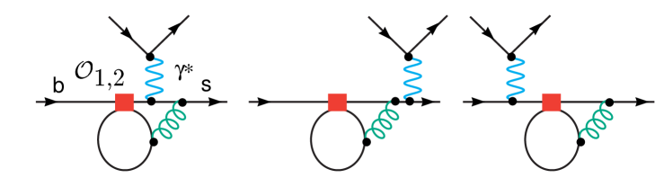
b)

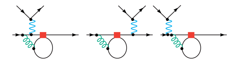
c)

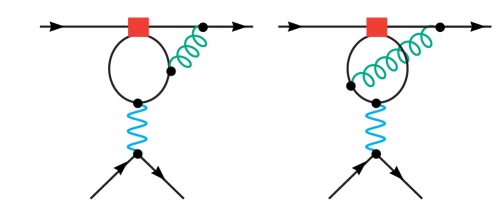
d)

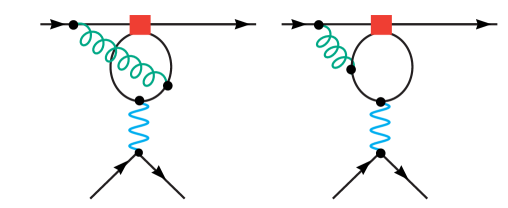
e)

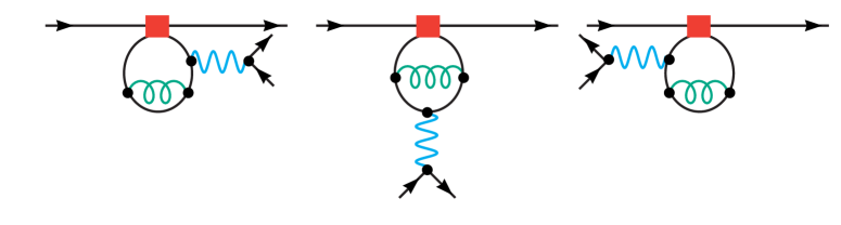
Figure 1: Two-loop Feynman diagrams relevant for the virtual QCD corrections corresponding to the operators ${\cal O}_{1}$ and ${\cal O}_{2}$. They can be organized in five gauge invariant subsets.

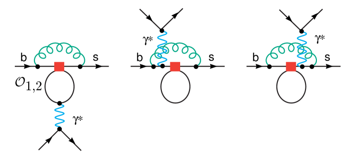
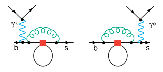
Figure 2: Two-loop Feynman diagrams relevant to the virtual QCD corrections corresponding to the operators ${\cal O}_{1}$ and ${\cal O}_{2}$, which can effectively be taken into account by a redefinition of the Wilson coefficients.

This is most effectively done by the redefinition of the Wilson coefficient (see A.4 in the appendix). When calculating the corrections to the operator ${\cal O}_{9}$ using these modified Wilson coefficients, the contributions of the diagrams given in 2 are automatically taken into account. We also note that by gauge invariance the QCD corrections to the matrix elements of the operators ${\cal O}_{1,2}$ can be written as

$$\langle s\ell^{+}\ell^{-}|{\cal O}_{i}\,|b\rangle=-\frac{\alpha_{s}}{4\pi}\left(F_{i}^{(9)}\langle\tilde{\cal O}_{9}\rangle_{tree}+F_{i}^{(7)}\langle\tilde{\cal O}_{7}\rangle_{tree}\right).$$ (3.1)

3.2 Method

Within the $B\rightarrow X_{s}\gamma$ calculation at NLL, the two-loop matrix elements of the four-quark operators ${\cal O}_{1}$ and ${\cal O}_{2}$ for an on-shell photon were calculated in [15] using Mellin–Barnes techniques. This calculation was extended in [6] to the case of an off-shell photon with the help of a double Mellin–Barnes representation. We are reminded that these matrix elements form an integral part of the NNLL analysis of the decay $B\rightarrow X_{s}\ell^{+}\ell^{-}$. The double expansion is in the dilepton mass $s=q^{2}/m_{b}2$ and the mass ratio $m^{2}_{c}/m^{2}_{b}$. Thus, the validity of the analytical results given in [6] is restricted to small dilepton masses $s<0.25$, because $c\bar{c}$ thresholds will be crossed beyond that.

We follow here a different strategy to calculate these two-loop matrix elements for arbitrary dilepton mass in our present NNLL work. We use a universal method, which can evaluate any two-loop diagrams of general external kinematics and internal masses semi-numerically. For its implementation, the diagrams are processed with a computer algebra program. The aim of the various algebraic manipulations to follow is to render the diagrams to a standard form, which will be further integrated numerically in the second stage of the analysis. We used two independent versions written in FORM and in Schoonship, which provide a powerful check on the algebra and consistency. Let us describe the individual steps of the calculation in more detail.

First, all two-loop diagrams are converted into sums of sun set type integrals and their mass derivatives:

$$\int d^{n}p\,d^{n}q\,\frac{p^{\mu_{1}}\ldots p^{\mu_{i}}q^{\mu_{i+1}}\ldots q^{\mu_{j}}}{((p+k)^{2}+m_{1}^{2})^{\alpha_{1}}(q^{2}+m_{2}^{2})^{\alpha_{2}}(r^{2}+m_{3}^{2})^{\alpha_{3}}},$$ (3.2)

where $r=p+q$, and $p$ and $q$ are the two independent internal momenta. This is done by the use of Feynman parameters $\{X\}$ and appropriate shifts in the variables $p$ and $q$.

Figure 3: Expressing generic massive two-loop Feynman diagrams as integrals over sunset-type functions.

The effective masses $m_{1,2,3}^{2}$ and the effective momentum $k$ are polynomial functions of physical masses, external kinematics, and Feynman parameters associated with the diagrams (see Fig. 3). By using mass derivatives, there is in principle only one basic set arising from [$\alpha_{1}=\alpha_{2}=\alpha_{3}=1$] we need to know, although we shall instead use [$\alpha_{1}=2,\alpha_{2}=\alpha_{3}=1$] as the basic set. The reason for the latter choice is that this set is less singular and it allows for neater integral representation of the corresponding scalar integrals, which makes them more suitable for numerical evaluation.

The second analytic step includes Lorentz decomposition of the tensor structures and isolation of the scalar integrals, and use of differential recursion relations to reduce the scalar functions to a set of ten master scalar functions. The tensor reduction is done by decomposing the loop momenta $p$ and $q$ in the numerator into components parallel and orthogonal to the external momentum $k$,

$$p_{\perp}^{\mu}=p^{\mu}-{p\cdot k\over k^{2}}k^{\mu},\ \ q_{\perp}^{\mu}=q^{\mu}-{q\cdot k\over k^{2}}k^{\mu}.$$ (3.3)

Tensor integrals with an odd number of transverse loop momenta $p_{\perp}$ and $q_{\perp}$ vanish, while the even ones will be contracted basically with the metric tensor for further simplification. The resulting scalar coefficients of the tensor decomposition are integrals of the following form:

$$\tilde{P}^{ab}_{211}(m_{1}^{2},m_{2}^{2},m_{3}^{2};k^{2})=\int d^{n}pd^{n}q{(p\cdot k)^{a}(q\cdot k)^{b}\over[(p+k)2+m_{1}^{2}]^{2}(q^{2}+m_{2}^{2})((p+q)^{2}+m_{3}^{2})},$$ (3.4)

where $a+b\leq 3$ in renormalizable theories; tensor integrals with more than three Lorentz indexes can be derived in a similar fashion but will not be needed. In general, one can prove [26] that any two-loop diagram in renormalizable theories can be decomposed by this algorithm into an expression involving only ten scalar integrals, denoted by ${\cal H}_{i},\,\,i=1\cdots 10$ in the following. They are linear combinations of integrals of the form (3.4) with $a+b\leq 3$. Let us reiterate that given enough computing power and up to possible infrared issues, which we shall mention below, the algorithm is applicable to any two-loop process.

After this algebra step, the ten scalar integrals are integrated over $p$ and $q$. An important feature is that the UV poles are isolated and one arrives at one-dimensional finite integral representations over a variable $0\leq x\leq 1$ of four elementary functions of $m_{1,2,3}^{2},k^{2}$ and $x$, which makes their numerical evaluation highly efficient and precise. As anticipated above, for this latter step our special choice $\alpha_{1}=2,\alpha_{2}=\alpha_{3}=1$ as a basis of integrals is crucial; with this choice the ten basic scalar integrals ${\cal H}_{i}$ are logarithmically divergent in the ultraviolet and these UV divergences are distinctly separate and manifestly exposed. The remaining finite parts, denoted by $h_{i}$, possess one-dimensional integral representations and will be displayed explicitly in an appendix. The kernels of $h_{i}$ are, interestingly enough, moments in the variable $x$ of four elementary functions:

$$\tilde{g}(m_{1},m_{2},m_{3};k^{2};x) = Sp(\frac{1}{1-y_{1}})+Sp(\frac{1}{1-y_{2}})+y_{1}\log{\frac{y_{1}}{y_{1}-1}}+y_{2}\log{\frac{y_{2}}{y_{2}-1}}$$

$$\tilde{f_{1}}(m_{1},m_{2},m_{3};k^{2};x) = \frac{1}{2}\left[-\frac{1-\mu^{2}}{\kappa^{2}}+y_{1}^{2}\log{\frac{y_{1}}{y_{1}-1}}+y_{2}^{2}\log{\frac{y_{2}}{y_{2}-1}}\right]$$

$$\tilde{f_{2}}(m_{1},m_{2},m_{3};k^{2};x) = \frac{1}{3}\left[-\frac{2}{\kappa^{2}}-\frac{1-\mu^{2}}{2\kappa^{2}}-\left(\frac{1-\mu^{2}}{\kappa^{2}}\right)^{2}+y_{1}^{3}\log{\frac{y_{1}}{y_{1}-1}}+y_{2}^{3}\log{\frac{y_{2}}{y_{2}-1}}\right]$$

$$\tilde{f_{3}}(m_{1},m_{2},m_{3};k^{2};x) = \frac{1}{4}\left[-\frac{4}{\kappa^{2}}-\left(\frac{1}{3}+\frac{3}{\kappa^{2}}\right)\left(\frac{1-\mu^{2}}{\kappa^{2}}\right)-\frac{1}{2}\left(\frac{1-\mu^{2}}{\kappa^{2}}\right)^{2}-\left(\frac{1-\mu^{2}}{\kappa^{2}}\right)^{3}\right.$$ (3.5)

$$\left.\;\;\;\;\;\;\;\;\;\;\;\;\;\;\;\;\;\;\;\;\;\;\;\;\;\;\;\;\;\;\;\;\;\;\;\;+y_{1}^{4}\log{\frac{y_{1}}{y_{1}-1}}+y_{2}^{4}\log{\frac{y_{2}}{y_{2}-1}}\right]\;\;,$$

$$y_{1,2}=\frac{1+\kappa^{2}-\mu^{2}\pm\sqrt{\Delta}}{2\kappa^{2}},\quad\quad\Delta=(1+\kappa^{2}-\mu^{2})^{2}+4\kappa^{2}\mu^{2}-4i\kappa^{2}\eta\;\;,$$

$$\mu^{2}=\frac{ax+b(1-x)}{x(1-x)}\,,\,\,\,a=\frac{m_{2}^{2}}{m_{1}^{2}}\,,\;\;\;\;b\;=\;\frac{m_{3}^{2}}{m_{1}^{2}}\,,\;\;\;\;\kappa^{2}\;=\;\frac{k^{2}}{m_{1}^{2}}\;\;.$$

Once the analytical procedure is done as described, each original Feynman diagram is expressed as an integral over the set of Feynman parameters $\{X\}$ introduced earlier. The integrand itself consists of a sum of the special functions $h_{i}$ (which are themselves one-dimensional integrals of the four elementary functions (3.2)) and possibly also of some trivial functions such as logarithms and rational functions of the kinematical invariants $m^{2}_{1,2,3},$ and $k^{2}$. Within our method, all these integrations generally are to be performed numerically. We shall not dwell on the details here. Suffice it to say that the analytic structure of the functions $h_{i}$ is well understood, so that the integration paths $\{{\it C\}}$ can be moved into complex planes to effect better numerical convergence and, more importantly, to yield amplitudes on the physical sheet. Because we are interested in a high accuracy and efficiency routine, we have used an adaptive deterministic integration algorithm. Such integration routines are very accurate, provided that the integrand is smooth enough and that the dimensionality of the integral is not too large. The integrand itself is, of course, an analytic function along any properly chosen complex integration path of $\{{\it C\}}$, and therefore in order to preserve this smoothness, it is advantageous to optimize the choice for a smooth integration path in the numerical work as well. One should be made aware that the integrals over Feynman parameters must be performed along a complex integration path that is consistent with the causality condition. This path is computed automatically by using spline functions such that both the path itself and its Jacobian are smooth functions. Moreover, we note that, in the problem at hand, we shall be dealing with three-fold numerical integrations at most.

We would like to mention that we perform minimal subtractions on all divergent subgraphs. We have checked that the anomalous dimensions so obtained for the operator mixing matrix elements agree with what is known in the literature. This will be further elaborated in a subsequent section. We have explicitly checked that each group of diagrams is gauge-invariant and have been further reassured by their numerical stability.

In the case of the calculation of the two-loop matrix elements of $B\rightarrow X_{s}\ell^{+}\ell^{-}$ decay, we deal with three kinematic variables: the charm mass, the dilepton invariant mass, and the subtraction scale. In order for the result to be usable for phenomenological studies, in particular to be implementable into a Monte Carlo simulation, we need to cover this three-dimensional kinematic space. A real-time calculation of the two-loop matrix element by numerical integration is far too slow to be implemented directly into a Monte Carlo simulation of the experimental set-up. With the present-day processors, an alternative of calculating in advance a comprehensive grid of integration points that cover the whole three-dimensional kinematic range, storing them, and then interpolating between them, seems to be the most efficient way because of the semi-numerical nature of our whole approach. All these considerations led us into writing a program that calculates the two-loop matrix elements efficiently and accurately, and which is fast enough to be incorporated into a Monte Carlo simulation. We selected a grid of $38\times 3\times 3$ integration points for both the electric and the magnetic components of the two-loop virtual corrections. Each of the 684 integration point yielding values for the form factors was calculated with a relative precision of $10^{-3}$. We used the CERN Linux cluster to perform this calculation, and the CPU usage was approximately 3 days on 33 processors (mostly 850 MHz) running in parallel.

Finally, we would like to mention a caveat in the semi-numerical algorithm presented here. In a general process, infrared singularities will most likely occur and will lead to infrared divergences in our integral representations. In such cases, it is more efficient to first separate out the infrared parts of the two-loop diagrams in an analytically manageable form. Fortunately, for the process at hand all relevant diagrams (a)–(e) in Fig. 1 are infrared-finite; therefore the algorithm is most suitable for this specific application.

3.3 Unrenormalized results

In the following we show plots of our results for the finite ($\epsilon^{0}$) parts of the unrenormalized (naked) two-loop Feynman diagrams of Fig. 1, which give matrix elements to the operators ${\cal O}_{1}$ and ${\cal O}_{2}$ within the $\overline{MS}$ scheme. The finite counterterm contributions are not included here but will be discussed in the next subsection. Our main purpose is to compare our results with those of Ref. [6] where Mellin–Barnes expansion techniques were used.

Each plot in Fig. 4 represents one of the five gauge-invariant diagram subsets given in Fig. 1. We want to bring attention to the complete range of the dilepton mass spectrum $s=[0,1]$ in all the plots, which is a salient point of this discussion. For each we plot the electric ($F^{(7)}$) and the magnetic ($F^{(9)}$) contributions, defined in (3.1) separately in the left and right columns, except for the subset (e), which has no contribution in the first column. The calculation of Asatrian et al. is shown as successive approximations, showing that it converges toward our result. Their results are valid only under the $c\bar{c}$ threshold, which we demarcate by vertical lines in the figures. Generally, the real part of our results is given by a solid line and the imaginary part by a dashed line. All the other lines are successive approximations in the momentum expansion series of Asatrian et al..

In Fig. 5 we zoom in to magnify the way the momentum expansion converges toward our exact numerical solution within the low-$s$ region. Here the stars are the actual points obtained from our numerical output, which are joined by the continuous lines obtained from the interpolation program.

The comparison can be summarized as follows: there is good agreement between our results for each diagram set and the double expansion of Asatrian et al. in the region below the $c\bar{c}$ threshold. This agreement within the low-$s$ region provides a strong confirmation of our numerical method. One notices that, as a general rule, the less singular the threshold behaviour of the diagram is, the better the momentum expansion converges toward our exact numerical result. For subsets (a) and (b) the expansion converges best because of the lack of a nontrivial threshold. For (c) and (d) the threshold is relatively mild, and the convergence is intermediary. For the gauge-invariant subset (e), the threshold is quite singular and thus we notice the poorest convergence of the momentum expansion. This singular behaviour is mostly due to the charm self-energy-type diagrams, as evidenced by a much milder disagreement of the two methods after the mass counterterm is added. This also makes the agreement between our final physical result and the momentum expansion result better than what can be inferred from Fig. 5 alone. The actual agreement of the two calculations within the low-$s$ region is compatible with the error of our numerical integration accuracy. We may find it interesting that, for the gauge-invariant subsets (a) and (b) the expanded results of [6] are actually valid beyond the $c\bar{c}$ threshold, perhaps because these diagrams have no threshold cuts in the way.

Before leaving this subsection, we want to remark that by our method we have reproduced numerically the values given by the analytical results on the two-loop matrix elements of ${\cal O}_{1,2}$ in the $B\rightarrow X_{s}\gamma$ mode presented in [15], with an accuracy well below $1\%$.

Figure 4: Plots of the UV-finite part of the Feynman diagram subsets shown in Fig. 1. The two columns correspond to the electric and the magnetic form factors; see (3.1). There is no electric contribution from the diagrams 1 e). We plot the real (solid line) and the imaginary (dashed line) parts of our exact numerical integration result, along with successive approximations in the momentum expansion series of the result of Asatrian et al. which is shown only below the $c\bar{c}$ threshold. For more details see main text.

Figure 5: Convergence pattern of the momentum expansion solution of Asatrian et al. toward our numerical integration solution. The stars denote actual integration points, and the solid line connecting them is an interpolation. For more details see main text.

3.4 Counterterm contributions

The counterterms to the matrix elements of the operators ${\cal O}_{1}$ and ${\cal O}_{2}$ will serve two purposes. They give renormalization to the QCD parameters and they account for operator renormalization due to mixing. Although the counterterms expanded in the variable $s$ can be found in [6], for us we need to generalize to arbitrary dilepton mass. Before giving our new final analytical results, we commence with a short discussion of the various bits and pieces that must be put together. We follow the conventions in [6], including the convention $d=4-2\,\epsilon$ and their convention regarding the evenescent operators. The anomalous dimensions describing the operator mixing are known (see [17, 6, 18]) and are given in the appendix. We take this opportunity to point out a very useful feature of our semi-numerical method in that the UV divergences are separated and given analytically through the whole calculation. Because of this, we were able to check the two-loop mixing results explicitly.

The list of non-trivial counterterm contributions to the functions $F_{i}^{(9)}$ and $F_{i}^{(7)}$ in (3.1), which are add to those from the naked diagrams given in Fig. 1, is the following:

• The two operators ${\cal O}_{1}$ and ${\cal O}_{2}$, which non-trivially mix into the four-quark operators at the one-loop level, inducing additional counterterm contributions. We denote them by $F_{i\rightarrow{4quark}}^{(7)}$ and $F_{i\rightarrow{4quark}}^{(9)}$. They are given by

  $$\sum_{j}\frac{\alpha_{s}}{4\pi}\frac{1}{\epsilon}a_{ij}^{11}\langle s\ell^{+}\ell^{-}|{\cal O}_{j}|b\rangle_{one-loop}=-(\frac{\alpha_{s}}{4\pi}(F_{i\rightarrow{4quark}}^{(7)}\langle\tilde{\cal O}_{7}\rangle_{tree}+F_{i\rightarrow{4quark}}^{(9)}\langle\tilde{\cal O}_{9}\rangle_{tree})),$$ (3.6)

  in which $j$ runs over all four-quark operators. This expression instructs us to calculate the one-loop matrix elements of the four-quark operators up to the $\epsilon^{1}$ terms for arbitrary dilepton mass.

• The analogous one-loop mixing of the operators ${\cal O}_{1}$ and ${\cal O}_{2}$ into ${\cal O}_{9}$. They are from the two-loop diagrams shown in Fig. 2.

• The one and two-loop mixing into ${\cal O}_{9}$, which is connected with the renormalization of the explicit coupling constant in the definition of ${\cal O}_{9}$. They appear in the diagrams of Fig. 1. This leads to an additional contribution to $F_{i}^{(9)}$ (but not $F_{i}^{(7)}$) in (3.1), which we call $F_{i\rightarrow{9}}^{(9)}$. It is given by

  $$F_{i\rightarrow 9}^{(9)}=-(\frac{a_{i9}^{22}}{\epsilon^{2}}+\frac{a_{i9}^{12}}{\epsilon})-\frac{a_{i9}^{11}\,\beta_{0}}{\epsilon^{2}},$$ (3.7)

  where we have used the coupling renormalization

  $$Z_{g_{s}}=1-\frac{\alpha_{s}}{4\pi}\,\frac{\beta_{0}}{2}\,\frac{1}{\epsilon}+O(\alpha_{s}^{2})\quad\mbox{with}\,\,\beta_{0}=11-\frac{23}{3}\quad\mbox{for five active flavours}.$$ (3.8)

• Then, there are QCD mass counterterm contributions from the renormalization of the charm mass within the matrix elements of ${\cal O}_{1}$ and ${\cal O}_{2}$, which we denote by $F_{i,m_{c}}^{(9)}$ and $F_{i,m_{c}}^{(7)}$. They are most easily given by replacing the charm mass $m_{c}$ by $Z_{m_{c}}\times m_{c}$ in the one-loop matrix elements of ${\cal O}_{1}$ and ${\cal O}_{2}$. We use the pole mass renormalization in our calculation:

  $$Z_{m_{c}}=1-\frac{\alpha_{s}}{4\pi}\frac{4}{3}\left(\frac{m_{b}^{2}}{\mu^{2}}\right)^{-\epsilon}\left(\frac{3}{\epsilon}+4\right)+O(\alpha_{s}^{2}),$$ (3.9)

In the following, we give the complete finite ($\epsilon^{0}$) counterterm contributions from the two-loop diagrams in Fig. 1. We write down our new final results for the relevant finite ($\epsilon^{0}$) parts for arbitrary dilepton mass:

$$F^{(k)}_{i,ct}=F_{i\rightarrow 9}^{(k)}+F_{i\rightarrow 4quark}^{(k)}+F_{i,m_{c}}^{(k)},\quad k=7,9\,,i=1,2.$$ (3.10)

$$F^{(7)}_{1,ct}\,\,|_{\epsilon^{0}} = \frac{4}{81}l_{\mu}+\frac{4}{81}B(s)$$ (3.11)

$$F^{(7)}_{2,ct}\,\,|_{\epsilon^{0}} = -\frac{8}{27}l_{\mu}-\frac{8}{27}B(s)$$

$$F^{(9)}_{1,ct}\,\,|_{\epsilon^{0}} = i\pi\left[\frac{8}{243}l_{s}+\frac{8}{243}l_{\mu}-\frac{16}{729}\right]+\frac{16}{729}l_{s}+\frac{704}{81}l_{c}-\frac{3560}{2187}-\frac{4}{243}l_{s}^{2}-\frac{8}{243}l_{s}l_{\mu}\qquad$$

$$+\frac{16}{27}l_{c}l_{\mu}+\frac{256}{9}C_{x}(s_{c})l_{\mu}+\frac{32}{9}B_{x}(s_{c})l_{c}+\frac{32}{9}B_{x}(s_{c})l_{\mu}+\frac{256}{9}C_{x}(s_{c})l_{c}$$

$$+\frac{256}{9}C_{xx}(s_{c})l_{c}-\frac{256}{9}C_{xx}(s_{c})l_{\mu}+\frac{6328}{729}l_{\mu}-\frac{32}{9}B_{xx}(s_{c})l_{\mu}-\frac{32}{9}B_{xx}(s_{c})l_{c}$$

$$+\frac{16}{81}B_{xx}(s)-\frac{16}{81}B_{x}(s)-\frac{8}{81}B_{2x}(s)+\frac{16}{9}B_{2x}(s_{c})-\frac{640}{27}B_{xx}(s_{c})+\frac{640}{27}B_{x}(s_{c})$$

$$+\frac{16}{243}\pi^{2}+\frac{8}{81}B_{2xx}(s)-\frac{16}{9}B_{2xx}(s_{c})+\frac{128}{27}C_{xx}(s_{c})+\frac{64}{9}C_{2x}(s_{c})$$

$$-\frac{64}{9}C_{2xx}(s_{c})-\frac{16}{81}l_{\mu}B_{x}(s)+\frac{16}{81}l_{\mu}B_{xx}(s)+\frac{64}{243}l^{2}_{\mu}-\frac{128}{27}C_{x}(s_{c})$$

$$F_{2,ct}^{(9)}\,\,|_{\epsilon^{0}} = i\pi\left[\frac{32}{243}-\frac{16}{81}l_{\mu}-\frac{16}{81}l_{s}\right]-\frac{32}{243}l_{s}+\frac{32}{27}l_{c}+\frac{8}{81}l_{s}^{2}+\frac{16}{81}l_{s}l_{\mu}-\frac{16}{9}l^{2}_{c}-\frac{32}{9}l_{c}l_{\mu}$$ (3.14)

$$+\frac{64}{3}C_{x}(s_{c})l_{\mu}-\frac{64}{3}B_{x}(s_{c})l_{c}-\frac{64}{3}B_{x}(s_{c})l_{\mu}+\frac{64}{3}C_{x}(s_{c})l_{c}-\frac{64}{3}C_{xx}(s_{c})l_{c}$$

$$-\frac{64}{3}C_{xx}(s_{c})l_{\mu}+\frac{304}{243}l_{\mu}+\frac{64}{3}B_{xx}(s_{c})l_{\mu}+\frac{64}{3}B_{xx}(s_{c})l_{c}-\frac{32}{27}B_{xx}(s)+\frac{32}{27}B_{x}(s)$$

$$+\frac{16}{27}B_{2x}(s)-\frac{32}{3}B_{2x}(s_{c})+\frac{128}{9}B_{xx}(s_{c})-\frac{128}{9}B_{x}(s_{c})-\frac{32}{81}\pi^{2}-\frac{16}{27}B_{2xx}(s)$$

$$+\frac{32}{3}B_{2xx}(s_{c})+\frac{32}{9}C_{xx}(s_{c})+\frac{16}{3}C_{2x}(s_{c})-\frac{16}{3}C_{2xx}(s_{c})+\frac{32}{27}l_{\mu}B_{x}(s)$$

$$-\frac{32}{27}l_{\mu}B_{xx}(s)-\frac{128}{81}l^{2}_{\mu}-\frac{32}{9}C_{x}(s_{c})-\frac{656}{729}$$

The functions $B(a)$, $B_{x}(a)$, $B_{xx}(a)$, $B_{2}(a)$, $B_{2x}(a)$, $B_{2xx}(a)$ and also the functions $C(a)$, $C_{x}(a)$, $C_{xx}(a)$, $C_{2}(a)$, $C_{2x}(a)$, $C_{2xx}(a)$ are defined in the appendix. We have also introduced the variable $s_{c}=q^{2}/m_{c}^{2}$ and we have defined $l_{\mu}=\ln(m_{b}^{2}/\mu^{2})$, $l_{c}=\ln(m_{c}^{2}/m_{b}^{2})$, and $l_{s}=\ln(s)$.

We have explicitly checked that all the $\epsilon^{-2}$ and $\epsilon^{-1}$ terms coincide with the results given in [6].

4 Calculation of the $O(\alpha_{s})$ virtual corrections to the
matrix element of ${\cal O}_{8}$

We present here a short description of our new calculation of the matrix element of the operator ${\cal O}_{8}$ for general $s$. Besides the contributions from the naked diagrams shown in Fig. 6, there is also a counterterm contribution due to the mixing of ${\cal O}_{8}$ into ${\cal O}_{7}$:

$$\langle s\ell^{+}\ell^{-}|\delta Z_{87}\,{\cal O}_{8}|b\rangle,\quad\quad\delta Z_{87}=-\frac{\alpha_{s}}{4\pi}\frac{16}{9\epsilon}\,.$$ (4.15)

The functions $F_{8}^{(7)}$ and $F_{8}^{(9)}$ in (2.7) are then defined by the renormalized matrix element of ${\cal O}_{8}$:

$$\langle s\ell^{+}\ell^{-}|C_{8}{\cal O}_{8}|b\rangle={C}_{8}^{(1)}(-\frac{\alpha_{s}}{4\pi})(F_{8}^{(9)}\langle\tilde{\cal O}_{9}\rangle_{tree}+F_{8}^{(7)}\langle\tilde{\cal O}_{7}\rangle_{tree}),$$ (4.16)

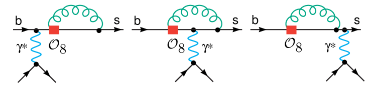
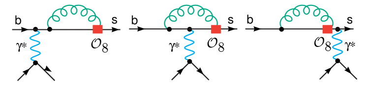
Figure 6: One-loop Feynman diagrams relevant to the virtual QCD corrections corresponding to the operators ${\cal O}_{8}$.

Keeping the full $s$ dependence, we find

$$F_{8}^{(7)} = -\frac{32}{9}\ln\left(\frac{\mu}{m_{b}}\right)-\frac{4}{27}\pi^{2}-\frac{4}{9}-\frac{8}{9}i\pi+\frac{8}{9}\frac{s\ln(s)}{s-1}$$ (4.17)

$$+\frac{4}{9}\int_{0}^{1}dx\int_{0}^{1-x}dy~{}\left[(7-3x-6y)\ln\left(1-s\frac{xy}{x^{2}+xy+y}\right)\right.$$

$$\qquad\qquad\left.-\frac{x^{3}+3x^{2}y+2xy^{2}-xy-s(x^{2}y+2xy^{2}-3xy)}{x^{2}+xy+y-sxy}\right]~{},$$

$$sF_{8}^{(9)} = \frac{8}{27}\pi^{2}-\frac{88}{27}-\frac{16}{9}\frac{s\ln(s)}{s-1}$$ (4.18)

$$+\frac{8}{9}\int_{0}^{1}dx\int_{0}^{1-x}dy~{}\left[-2(2-3x-3y)\ln\left(1-s\frac{xy}{x^{2}+xy+y}\right)\right.$$

$$\quad\left.+\frac{2x^{3}+4x^{2}y+2xy^{2}-x^{2}-xy+y-s(2xy^{2}+2x^{2}y-3xy+y)}{x^{2}+xy+y-sxy}\right]~{}.\quad$$

If we expand our results for small $s$, we recover the results given in [6].

5 Non-perturbative contributions

5.1 Generalities

Non-perturbative contributions in $B\to X_{s}\ell^{+}\ell^{-}$ transitions can be divided into two main categories:

• $\Lambda_{\rm QCD}/m_{b}$ corrections in the relation between the partonic $b\to s\ell^{+}\ell^{-}$ amplitude and inclusive hadronic distributions;

• non-perturbative effects associated with the $c\bar{c}$ intermediate state: $B\to X_{s}c\bar{c}\to X^{\prime}_{s}\ell^{+}\ell^{-}$.

The heavy-quark expansion, which led us to evaluate the first type of contributions, is rapidly convergent and leads to small corrections for sufficiently inclusive observables. A consistent treatment of the second type of effects requires to impose kinematical cuts to avoid the large non-perturbative background of the narrow $c\bar{c}$ resonances. These two requirements are somehow in conflict. As a result, we can perform reliable predictions of $B\to X_{s}\ell^{+}\ell^{-}$ transitions, both in the low- and in the high-$q^{2}$ regions, but magnitude and error of the non-perturbative corrections are enhanced with respect to their natural size.

The enhancement of $\Lambda_{\rm QCD}/m_{b}$ corrections is particularly sizeable in the high-$q^{2}$ region, because of two main drawbacks:

• the $1/m_{b}$ expansion breaks down in the limit $q^{2}\to m^{2}_{b}$ [24, 27];

• the $q^{2}$ cut introduces a sizeable effective correction linear in $1/m_{b}$, through the relation between hadronic and partonic phase spaces.

The first problem implies that in the high-$q^{2}$ region the differential distribution in $q^{2}$ cannot be predicted in perturbation theory. This non-perturbative distribution has nothing to do with the so-called shape function, or the kinetic energy distribution of the heavy quark inside the hadron [27]. However, similarly to the latter, the $q^{2}$ distribution near the end point is a non-perturbative function, which must be determined from data. What can still be predicted with reasonable accuracy, for a sufficiently low cut-off $q_{\rm min}^{2}$, is the $q^{2}>q_{\rm min}^{2}$ integral (or the full inclusive distribution for $q^{2}>q_{\rm min}^{2}$).

The second drawback is common to all observables that require kinematical cuts (in practice to any experimentally accessible inclusive observable in $B$ decays). Since any kinematical cut on the final state must be expressed in terms of the hadron mass $M_{B}$, we cannot avoid the linear $1/m_{b}$ corrections that arises from the relation

$$M_{B}=m_{b}\left[1+\frac{\bar{\Lambda}}{m_{b}}-\frac{\lambda_{1}+3\lambda_{2}}{2m_{b}^{2}}+O\left(\frac{\Lambda_{\rm QCD}}{m_{b}^{3}},\alpha_{s}\right)\right]~{}.$$ (5.19)

This problem is substantially enhanced in the high-$q^{2}$ region because of the smallness of the available phase space: here the relative correction between the hadronic phase space [$\sim(M_{B}-\sqrt{q^{2}_{\rm min}})$] and the partonic one [$\sim(m_{b}-\sqrt{q^{2}_{\rm min}})$] becomes an $O(1)$ effect.

As we shall discuss in detail in the following, these two drawbacks fit within a common picture: the heavy-mass expansion in the high-$q^{2}$ region is an effective expansion in inverse powers of

$$m^{\rm eff}_{\rm heavy}=m_{b}\times(1-\sqrt{s_{\rm min}})~{},$$ (5.20)

rather than $m_{b}$. This expansion is justified, but it converges less rapidly than the usual series in $\Lambda_{\rm QCD}/m_{b}$.

5.2 $\Lambda^{2}_{\rm QCD}/m_{b}^{2}$ and $\Lambda^{3}_{\rm QCD}/m_{b}^{3}$ corrections

The $\Lambda_{\rm QCD}/m_{b}$ corrections can be systematically investigated in the framework of the heavy-quark expansion and, in particular, by means of the heavy-quark effective theory (HQET) [28]. The two main distributions, $R(s)$ and $A_{\rm FB}(s)$, are not affected by linear corrections and the leading effects of $O(\Lambda^{2}_{\rm QCD}/m^{2}_{b})$ can be described in terms of the two expectation values

$$\lambda_{1}=\frac{\langle B|\bar{h}(iD)^{2}h|B\rangle}{2M_{B}}~{},\qquad\lambda_{2}=\frac{1}{6}\frac{\langle B|\bar{h}g\sigma\cdot Gh|B\rangle}{2M_{B}}=\frac{M^{2}_{B^{*}}-M^{2}_{B}}{4}~{},$$ (5.21)

where $h$ is the heavy-quark field in the effective theory. The explicit expression of these corrections, which have been computed in Refs. [24, 27] (see also Ref. [29]), is

$$\delta_{1/m^{2}_{b}}R(s) = \frac{3\lambda_{2}}{2m^{2}_{b}}\Biggl{(}\frac{\alpha_{\rm em}^{2}}{4\pi^{2}}\left|\frac{V_{ts}}{V_{cb}}\right|^{2}\frac{1}{f(z)\kappa(z)}\Biggl{\{}-(6+3s-5s^{3})\frac{4|C^{\rm new}_{7}(s)|^{2}}{s}$$ (5.22)

$$\qquad+(1-15s^{2}+10s^{3})\left[|C^{\rm new}_{9}(s)|^{2}+|C^{\rm new}_{10}(s)|^{2}\right]$$

$$\qquad-4(5+6s-7s^{2})\mbox{Re}\left[C^{\rm new}_{7}(s)C^{\rm new}_{9}(s)^{*}\right]\Biggr{\}}+\frac{{g_{\lambda}(z)}}{f(z)}R(s)\Biggr{)}~{},\qquad$$

$$\delta_{1/m^{2}_{b}}A_{\rm FB}(s) = \frac{3\lambda_{2}}{2m^{2}_{b}}\Biggl{(}\frac{\alpha_{\rm em}^{2}}{4\pi^{2}}\left|\frac{V_{ts}}{V_{cb}}\right|^{2}\frac{1}{f(z)\kappa(z)}\Biggl{\{}s\mbox{Re}\left[C^{\rm new}_{10}(s)^{*}C^{\rm new}_{9}(s)\right](9+14s-15s^{2})$$ (5.23)

$$\qquad+2\mbox{Re}\left[C^{\rm new}_{10}(s)^{*}C^{\rm new}_{7}(s)\right](7+10s-9s^{2})\Biggr{\}}+\frac{{g_{\lambda}(z)}}{f(z)}A_{FB}(s)\Biggr{)}$$

$$\qquad+\frac{4\lambda_{1}}{3m^{2}_{b}}\frac{s}{(1-s)^{2}}A_{\rm FB}(s)~{}.\qquad$$

In both cases we have taken into account also the $1/m^{2}_{b}$ terms arising from the semileptonic normalization, namely

$$\Gamma(B\to X_{c}e\nu) = \frac{G^{2}_{F}m^{5}_{b}}{192\pi^{3}}|V_{cb}|^{2}f(z)\kappa(z)\left[1+\frac{\lambda_{1}}{2m^{2}_{b}}-\frac{3\lambda_{2}}{2m^{2}_{b}}\frac{{g_{\lambda}(z)}}{f(z)}\right]~{},$$ (5.24)

$${g_{\lambda}(z)} = {3-8z+24z^{2}-24z^{3}+5z^{4}+12z^{2}\ln z~{}.}$$ (5.25)

This normalization is responsible for the absence of explicit $O(\Lambda_{\rm QCD}/m_{b})$ corrections, since it cancels any explicit dependence from $m_{b}$, and it is also responsible for the absence of any dependence from the kinetic energy of the $b$-quark ($\sim\lambda_{1}$) in $R(s)$.

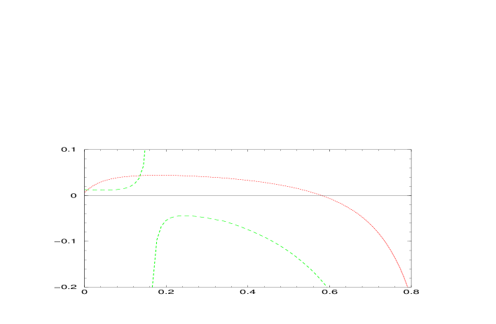
$s$

Figure 7: Relative corrections due $O(\Lambda^{2}_{\rm QCD}/m_{b}^{2})$ effects: $\delta_{1/m^{2}_{b}}R(s)/R(s)$ (dotted) and $\delta_{1/m^{2}_{b}}A_{\rm FB}(s)/A_{\rm FB}(s)$ (dashed).

As can be seen in Fig. 7, the relative corrections $\delta_{1/m^{2}_{b}}R(s)/R(s)$ and $\delta_{1/m^{2}_{b}}A_{\rm FB}(s)/A_{\rm FB}(s)$ are of the order of a few percent in the small $s$-region, apart from the obvious divergence in $\delta_{1/m^{2}_{b}}A_{\rm FB}(s)/A_{\rm FB}(s)$ due to the zero of $A_{\rm FB}(s)$ (the shift in the position of the zero amounts only to an increase of about $0.9\%$). However, in both cases the non-perturbative corrections become quite sizeable in the large $s$-region and the $1/m_{b}$ expansion breaks down close to the $s\to 1$ endpoint. The nature of this singularity has been discussed in detail in Ref. [27]. As usual, the HQET cannot be applied in corners of the phase space of $O(\Lambda_{\rm QCD}/m_{b})$, where the kinematics forces the final hadronic state to assume soft configurations. However, this particular case is rather different from the well-known examples of the photon-energy endpoint in $B\to X_{s}\gamma$, or the lepton-energy endpoint in $B\to X_{c}\ell\nu$. There only the hadronic invariant mass is constrained to be semi-soft $(k^{2}\sim m_{b}\Lambda_{\rm QCD})$ and the breakdown of the HQET is cured by means of a resummation of singular terms which leads to the shape function, or the universal non-perturbative distribution of the $b$-quark kinetic energy inside the hadron. Contrary to these examples, the kinematical constraint corresponding to the dilepton invariant-mass end-point, namely $m_{b}-\sqrt{q^{2}}=O(\Lambda_{\rm QCD})$, forces the hadronic system to have both soft momentum $(k\sim\Lambda_{\rm QCD})$ and soft $(k^{2}\sim\Lambda^{2}_{\rm QCD})$ invariant mass. This implies that no resummation can be applied and that the singularity has nothing to do with the kinetic-energy distribution of the $b$-quark [27].

The fact that the $O(\Lambda_{\rm QCD}/m_{b})$ corrections are not under control for $s\to 1$, does not prevent us from performing reliable predictions for the partially integrated branching ratio (and FB asymmetry) in the high-$s$ region, provided we choose a sufficiently low cut-off $s_{\rm min}$. The main issue is which is the maximal allowed value for $s_{\rm min}$.

Once we impose a constraint of the type $s>s_{\rm min}$, the inclusive sum on the hadronic final state is limited to systems with invariant mass up to the effective scale $m^{\rm eff}_{\rm heavy}$ in (5.20). For this reason, in this partially integrated observables we expect an effective expansion ruled by inverse powers of $m^{\rm eff}_{\rm heavy}$, rather than $m_{b}$. This naive expectation is confirmed by the detailed analysis of Ref. [30], applied $B\to X_{u}\ell\nu$ decays. There the dilepton-invariant-mass cut necessary to avoid the $B\to X_{c}\ell\nu$ background leads to an effective expansion in inverse powers of $m_{c}$, rather than $m_{b}$ [30].

$\bar{\Lambda}$	$\lambda_{1}^{\rm eff}$(GeV2)	$\lambda^{\rm eff}_{2}$(GeV2)	$\rho_{1}$(GeV3)
$0.40\pm 0.10$	$-0.15\pm 0.10$	$0.12\pm 0.02$	$0.06\pm 0.06$

Table 1: Input values of the HQET parameters used to estimate linear, quadratic and cubic corrections in the $1/m_{b}$ expansion.

Because of these general arguments, we expect that the expansion should still be reliable, although with a slower convergence, for $s_{\rm min}\stackrel{{\scriptstyle>}}{{{}_{\sim}}}0.6$ (corresponding to $m^{\rm eff}_{\rm heavy}\stackrel{{\scriptstyle>}}{{{}_{\sim}}}1$ GeV). To address this issue in a more quantitative way, we shall look at the explicit expression of the $\Lambda_{\rm QCD}^{3}/m^{3}_{b}$ corrections in $R(s)$ [31]. At this order we need to introduce seven new hadronic matrix elements. Five of them lead only to a redefinition of the $\Lambda_{\rm QCD}^{2}/m^{2}_{b}$ couplings $\lambda_{1,2}$. In particular, the contributions proportional to ${\cal T}_{1\ldots 4}$ and $\rho_{2}$, in the notation of Ref. [32], are obtained from Eqs. (5.22) and (5.23), with the replacement [31, 32]:

$$\lambda_{1}\to\lambda_{1}^{\rm eff}=\lambda_{1}+\frac{{\cal T}_{1}+3{\cal T}_{2}}{m_{b}},\qquad\lambda_{2}\to\lambda_{2}^{\rm eff}=\lambda_{2}+\frac{{\cal T}_{3}+3{\cal T}_{4}}{m_{b}}-\frac{\rho_{2}}{m_{b}}~{}.$$ (5.26)

These terms do not spoil the convergence of the $1/m_{b}$ expansions, independently of the $s_{\rm min}$ cut, provided the naive chiral-counting expectation ${\cal T}_{1\ldots 4}\sim\rho_{1,2}\sim\Lambda^{3}_{\rm QCD}$ is respected. More delicate is the issue of the contributions proportional to $\rho_{1}$ and $f_{1}$ [31]:

$$\delta_{1/m^{3}_{b}}R(s) = -\frac{\rho_{1}}{m^{3}_{b}}\Biggl{(}\frac{{g_{\rho}(z)}}{6f(z)}R(s)+\frac{\alpha_{\rm em}^{2}}{4\pi^{2}}\left|\frac{V_{ts}}{V_{cb}}\right|^{2}\frac{1}{f(z)\kappa(z)}\Biggl{\{}$$ (5.27)

$$\left[\frac{5s^{4}+19s^{3}+9s^{2}-7s+22}{6(1-s)}+8\Delta(f_{1})\delta(1-s)\right]\frac{4|C^{\rm new}_{7}(s)|^{2}}{s}$$

$$+\left[\frac{10s^{4}+23s^{3}-9s^{2}+13s+11}{6(1-s)}+8\Delta(f_{1})\delta(1-s)\right]\left[|C^{\rm new}_{9}(s)|^{2}+|C^{\rm new}_{10}(s)|^{2}\right]$$

$$+4\left[\frac{-3s^{3}+17s^{2}-s+3}{2(1-s)}+8\Delta(f_{1})\delta(1-s)\right]\mbox{Re}\left[C^{\rm new}_{7}(s)C^{\rm new}_{9}(s)^{*}\right]\Biggr{\}}\Biggr{)}~{},\qquad$$

where

$$g_{\rho}(z)=77-88z+24z^{2}-8z^{3}+5z^{4}+48\ln z+36z^{2}\ln z$$ (5.28)

arises from the semileptonic normalization and $\Delta(f_{1})$ is a local contribution that cures the singularity of $\int_{0}^{s}ds^{\prime}R(s^{\prime})$ for $s\to 1$. When integrated in the high-$s$ region, Eq. (5.27) leads to a huge coefficient for the $\rho_{1}/m^{3}_{b}$ correction, much larger than the already sizeable $\lambda_{2}/m^{2}_{b}$ term [31]. However, everything looks very reasonable, once we introduce the effective scale in (5.20). For $s_{\rm min}\approx 0.6$ we find

$$\int_{s_{\rm min}}^{1}ds~{}R(s)=\left[1-\frac{1.6\lambda_{2}}{m_{b}^{2}(1-\sqrt{s_{\rm min}})^{2}}+\frac{1.8\rho_{1}+1.7f_{1}}{m_{b}^{3}(1-\sqrt{s_{\rm min}})^{3}}\right]\times\int_{s_{\rm min}}^{1}ds~{}\left.R(s)\right|_{m_{b}\to\infty}~{},$$ (5.29)

which perfectly confirms our expectation of an effective expansion in inverse powers of $m^{\rm eff}_{\rm heavy}$. According to the input values in Table 1, which are consistent with recent experimental determinations (see e.g. Ref. [33]), and setting $f_{1}=0$, the numerical size of the term between square brackets in (5.29) is $[1-0.08\pm 0.08]$.

5.3 The $\bar{\Lambda}/m_{b}$ correction

As anticipated, even though $R(s)$ and $A_{\rm FB}(s)$ are not explicitly affected by linear corrections in the $1/m_{b}$ expansion, the physical observables defined in terms of a $q^{2}$ cut are sensitive to the $\bar{\Lambda}/m_{b}$ term via the relation (5.19). This term – or equivalently the uncertainty on the value of $m_{b}$ – represent at present the largest source of non-perturbative uncertainty in the high-$q^{2}$ region. Choosing as reference cut the value $s_{\rm min}=0.6$, the physical observable defined in terms of $q^{2}_{\rm min}$ can be written as

$$R_{\rm cut}(q^{2}_{\rm min}) = \int_{q^{2}>q^{2}_{\rm min}}dq^{2}\frac{d\Gamma(B\to X_{s}\ell^{+}\ell^{-})}{\Gamma(B\to X_{c}e\nu)}$$ (5.30)

$$= \left\{1-6.2\left(\frac{q^{2}_{\rm min}}{m_{b}^{2}}-0.6\right)+O\left[\left(\frac{q^{2}_{\rm min}}{m_{b}^{2}}-0.6\right)^{2}\right]\right\}\times\int_{0.6}^{1}ds~{}R(s)~{},$$

which implies

$$\frac{\delta R_{\rm cut}}{R_{\rm cut}}\approx 7.4\frac{\delta m_{b}}{m_{b}}~{}.$$ (5.31)

This means that an error $\delta m_{b}=0.1$ GeV (corresponding to the uncertainty on $\bar{\Lambda}$ in Table 1), leads to a $\approx 15\%$ error on $R_{\rm cut}$.

5.4 $1/m_{c}^{2}$ non-perturbative corrections

The second class of non-perturbative effects relevant in $B\to X_{s}\ell^{+}\ell^{-}$ decays are the long-distance corrections related to $c\bar{c}$ intermediate states. These originate from the non-perturbative interactions of the $c\bar{c}$ pair in the process $B\to X_{s}c\bar{c}\to X_{s}\ell^{+}\ell^{-}$. If the dilepton invariant mass is near the first two $J^{PC}=1^{--}$ $c\bar{c}$ resonances ($\Psi$ and $\Psi^{\prime}$), this effect is very large and shows up as a peak in $R(s)$. However, one can easily eliminate this background by suitable kinematical cuts. More delicate is the estimate of the long-distance effects away from the resonance peaks.

An interesting approach which avoid double-counting problems is the one proposed in Ref. [34] (KS approach). Here, in order to take into account charm rescattering, the correction to $C_{9}$ induced by $b\to c\bar{c}s$ operators is estimated by means of experimental data on $\sigma(e^{+}e^{-}\to c\bar{c}$ hadrons) using a dispersion relation. To be more specific, the function $h(z,s)$ appearing in (A.7) is replaced by

$$h(z,s)\longrightarrow h(z,0)+{s\over 3}P\int_{s_{c}}^{\infty}ds^{\prime}\frac{R^{c\bar{c}}_{\rm had}(s^{\prime})}{s^{\prime}(s^{\prime}-s)}+i\frac{\pi}{3}R^{c\bar{c}}_{\rm had}(s)~{},$$ (5.32)

where $R^{c\bar{c}}_{\rm had}(s)=\sigma(e^{+}e^{-}\to c\bar{c})/\sigma(e^{+}e^{-}\to\mu^{+}\mu^{-})$ and $s_{c}$ is the $c\bar{c}$ threshold. This method is exact only in the limit where the $\bar{B}\to X_{s}c\bar{c}$ transition can be factorized into the product of $\bar{s}b$ and $\bar{c}c$ colour-singlet currents (i.e. non-factorizable effects are not included). The non-perturbative corrections estimated using this approach are extremely small in the perturbative windows $s<0.25$ and $s>0.6$ [35]. For the integrated branching ratios one finds an increase of $1-2\%$ in the low-$s$ region, while the effect in the high-$s$ region is far below the uncertainty of the $1/m_{b}$ corrections.

A systematic and model-independent way to estimate the non-factorizable $c\bar{c}$ long-distance effects far from the resonance region is obtained by means of an expansion in inverse powers of the charm-quark mass [36, 37]. This approach, originally proposed in [38] to evaluate similar effects in $B\to X_{s}\gamma$ decays, has the advantage of dealing only with partonic degrees of freedom. In this framework the leading non-perturbative corrections to $R(s)$ and $A_{\rm FB}$ turn out to be $O(\Lambda^{2}_{\rm QCD}/m_{c}^{2})$; their explicit expressions can be found in the appendix. Since the factorizable corrections vanish for $s\to 0$, the $O(\Lambda^{2}_{\rm QCD}/m_{c}^{2})$ effect is expected to be the dominant long-distance contribution for small values of the dilepton invariant mass. In this region the relative magnitude is very small (at the $1$ or $2\%$ level) and opposite in sign to the factorizable KS correction. The $O(\Lambda^{2}_{\rm QCD}/m_{c}^{2})$ calculation should be reliable also above the resonance region ($s>0.6$), where the effect is again very small. Similar comments apply to the long-distance corrections for $A_{\rm FB}(s)$.

6 Phenomenological analysis

6.1 Branching ratio and dilepton invariant-mass spectrum

The final results of this work concerning the dilepton invariant-mass spectrum is summarized in Fig. 8. In the upper plot we compare our un-expanded result, without any non-perturbative correction, to the expanded result of Ref. [6]. As can be noted, the expanded result provides a perfect approximation to the full calculation up to about the $c\bar{c}$ threshold. This is of course a good cross-check of Ref. [6] and an important test of our method, which turns out to be essential to provide a reliable prediction in the high-$q^{2}$ region. The Fig. 8 also shows that the expanded result differs significantly from the exact NNLL result above the threshold as expected. Note that the scale dependence in the high-$q^{2}$ region is very small, therefore our NNLL result provides an excellent level of accuracy for the pure partonic calculation. The lower plot in Fig. 8 provides an illustration of the non-perturbative effects induced by $c\bar{c}$ intermediate states (evaluated using the KS approach, see Sect. 5.4). As can be noted, the point-by-point corrections in $q^{2}$ are quite sizeable in the high-$q^{2}$ window. As discussed in the previous section, only the $q^{2}$-integral can be predicted reliably in this region.

$m_{b}=(4.9\pm 0.1)$ GeV

$m_{c}/m_{b}=0.29\pm 0.02$

$\mu=\left(5.0^{+5.0}_{-2.5}\right)$ GeV

$\alpha_{s}(M_{Z})={0.119}$

$\alpha_{\rm em}=1/128$

$|V^{*}_{tb}V_{ts}/V_{cb}|=0.97$

$\overline{m_{t}}(m_{t})=167$ GeV

Table 2: Main input values used in the numerical analysis.

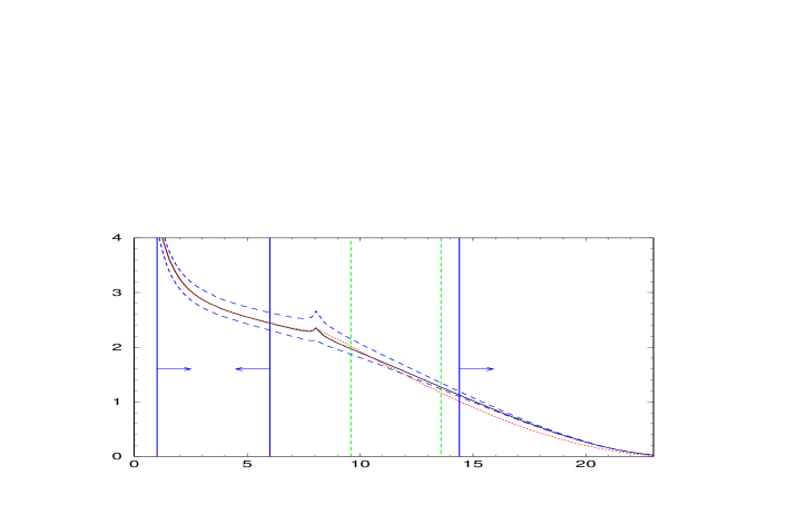
$\quad 10^{7}\times\displaystyle\frac{d{\cal B}}{dq^{2}}$ $\quad~{}({\rm GeV}^{-2})$

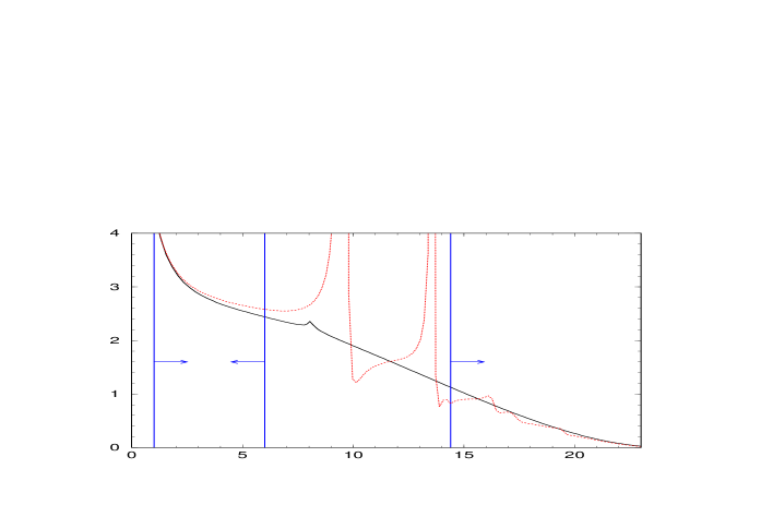
$\quad 10^{7}\times\displaystyle\frac{d{\cal B}}{dq^{2}}$ $\quad~{}({\rm GeV}^{-2})$
                                                                                                     $q^{2}~{}({\rm GeV}^{2})$

Figure 8: NNLL predictions of $d{\cal B}(B\to X_{s}\ell^{+}\ell^{-})/dq^{2}$. Upper plot: pure partonic result with full $m_{c}$ dependence computed in this work for $\mu$=5 GeV (full line), $\mu$=2.5 and 10 GeV (dashed lines); $q^{2}/(4m^{2}_{c})$-expanded result by Asatrian et al. [6], for $\mu$=5 GeV, extrapolated to the full $q^{2}$ range (dotted line); the dashed vertical lines indicate the positions of the first two narrow $\Psi$ resonances. Lower plot: partonic result with full $m_{c}$ dependence for $\mu$=5 GeV with (dotted line) or without (full line) factorizable $c\bar{c}$ corrections computed in the KS approach (see Sect. 5.4). All other inputs are fixed to the central values in Table 2

Before discussing the numerical predictions for the integrated branching ratios, we wish to emphasize that low- and high-$q^{2}$ regions have complementary virtues and disadvantages. Taking into account the discussion in the previous section, we can summarize the main points as follows:

• Virtues of the low-$q^{2}$ region: reliable $q^{2}$ spectrum; small $1/m_{b}$ corrections; sensitivity to the interference of $C_{7}$ and $C_{9}$; high rate.

• Disadvantages of the low-$q^{2}$ region: difficult to perform a fully inclusive measurement (severe cuts on the dilepton energy and/or the hadronic invariant mass); long-distance effects due to processes of the type $B\to\Psi X_{s}\to X_{s}+X^{\prime}\ell^{+}\ell^{-}$ not fully under control; non-negligible scale and $m_{c}$ dependence.

• Virtues of the high-$q^{2}$ region: negligible scale and $m_{c}$ dependence due to the strong sensitivity to $|C_{10}|^{2}$; easier to perform a fully inclusive measurement (small hadronic invariant mass); negligible long-distance effects of the type $B\to\Psi X_{s}\to X_{s}+X^{\prime}\ell^{+}\ell^{-}$.

• Disadvantages of the high-$q^{2}$ region: $q^{2}$ spectrum not reliable; sizeable $1/m_{b}$ corrections; low rate.

Given this situation, we believe that future experiments should try to measure the branching ratios in both regions and report separately the two results. These two measurements are indeed affected by different systematic uncertainties (of theoretical nature) and provide different short-distance information.

In order to obtain theoretical predictions which can be confronted with experiments, it is necessary to define the two regions with appropriate cuts in $q^{2}$ (and not in the partonic variable $s$, as done in most of the previous literature). Concerning the low-$q^{2}$ window, we propose as reference interval the range $q^{2}\in[1,6]~{}{\rm GeV}^{2}$. The lower bound on $q^{2}$ is not essential, but it proposed in order to cut a region where there is no new information with respect to $B\to X_{s}\gamma$ and where we cannot trivially combine electron and muon modes. The higher cut is essential to decrease the uncertainty associated to the $c\bar{c}$ threshold.

Taking into account the input values in Table 2, the NNLL prediction within the SM for this low-$q^{2}$ window is:

$$R^{\rm low}_{\rm cut} = \int_{1~{}{\rm GeV}^{2}}^{6~{}{\rm GeV}^{2}}dq^{2}\frac{d\Gamma(B\to X_{s}\ell^{+}\ell^{-})}{\Gamma(B\to X_{c}e\nu)}=1.48\times 10^{-5}$$ (6.33)

$$\times\Biggl{[}1\pm 8\%\big{|}_{\Gamma_{\rm sl}}\pm 6.5\%\big{|}_{\mu}\pm 2\%\big{|}_{m_{c}}\pm 3\%\big{|}_{m_{b}({\rm cuts})}+(4.5\pm 2)\%\big{|}_{1/m^{2}_{b}}-(1.5\pm 3)\%\big{|}_{c\bar{c}}\Biggl{]}$$

$$= (1.52\pm 0.18)\times 10^{-5}~{}.$$

Between square brackets we have reported all the uncertainties and non-perturbative corrections discussed in this work, evaluated according to the input values in Table 1 and 2. The error denoted by $\Gamma_{\rm sl}$ corresponds to the theoretical uncertainty implied by the $\Gamma(B\to X_{c}e\nu)$ normalization which, in turn, is dominated by the uncertainty on $m_{c}$. In principle, alternative normalizations such as the one proposed in Ref. [39] could be used to reduce this error. In any case, this uncertainty should be regarded as a parametric error which can be improved by additional independent measurements. The small error denoted by $m_{c}$ correspond to the $m_{c}$-dependence of $\Gamma(B\to X_{s}\ell^{+}\ell^{-})$ only (ignoring the normalization): as can be noted, this is almost negligible.

As already pointed out, our calculation of the matrix elements provides a completely independent check of the results of Ref. [6] for the low-$q^{2}$ region. In particular, we confirm the reduction of the scale uncertainty from $\pm 13\%$ to $\pm 6.5\%$, in the branching ratio, once these NNLL corrections are included (see Fig. 9). The difference in the central value of $R^{\rm low}_{\rm cut}$, compared to the result of Ref. [6], is entirely due a different definition of this observable and to differences in the input values.

Concerning the high-$q^{2}$ window, we propose as reference cut $q^{2}>14.4{\rm GeV}^{2}$, which leads to the following first NNLL prediction of the high dilepton mass spectrum:

$$R^{\rm high}_{\rm cut} = \int_{q^{2}>14.4~{}{\rm GeV}^{2}}dq^{2}\frac{d\Gamma(B\to X_{s}\ell^{+}\ell^{-})}{\Gamma(B\to X_{c}e\nu)}=4.09\times 10^{-6}$$ (6.34)

$$\times\Biggl{[}1\pm 8\%\big{|}_{\Gamma_{\rm sl}}\pm 3\%\big{|}_{\mu}+0.15\left(\frac{m_{b}-4.9~{}{\rm GeV}}{0.1~{}{\rm GeV}}\right)-(8\pm 8)\%\big{|}_{1/m^{(2,3)}_{b}}\pm 3\%\big{|}_{c\bar{c}}\Biggl{]}$$

$$= (3.76\pm 0.72)\times 10^{-6}~{}.\quad$$

Here the explicitly indicated $m_{b}$ dependence induces the largest uncertainty. At present this is about $15\%$. However, significant improvements can be expected in the near future in view of more precise data on other inclusive semileptonic distributions. Note that, as anticipated, in this region the pure perturbative uncertainties due to scale and $m_{c}$ dependence are very small (the latter has not been explicitly indicated being below 1%). The impact of the NNLL corrections computed in this work for the high $q^{2}$ region is a $13\%$ reduction of the central value and a significant reduction of the perturbative scale dependence (from $\pm 13\%$ to $\pm 3\%$, see Fig. 9).

As also shown in Fig. 9, this reduction brings the central value of the full NNLL prediction very close to the partial NNLL result obtained without the $F^{(7,9)}_{1,2,8}$ functions, provided in the latter case the renormalization scale is set around $2.5$ GeV. This observation, which has already been made in Ref. [40] for the low-$q^{2}$ window, applies remarkably well also in the high $q^{2}$ region. Obviously, our full NNLL calculation provides a fundamental ingredient to justify this procedure for the central value and, especially, to obtain a clear estimate of the residual scale uncertainty.

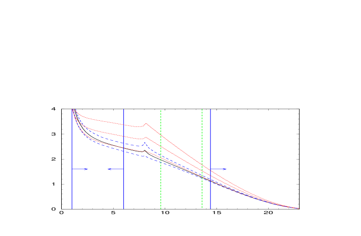
$\quad 10^{7}\times\displaystyle\frac{d{\cal B}}{dq^{2}}$ $\quad~{}({\rm GeV}^{-2})$
                                                                                                     $q^{2}~{}({\rm GeV}^{2})$

Figure 9: Complete NNLL result for $d{\cal B}(B\to X_{s}\ell^{+}\ell^{-})/dq^{2}$ for $\mu$=5 GeV (full line), $\mu$=2.5 and 10 GeV (dashed lines), vs. the partial NNLL result obtained by neglecting the $F^{(7,9)}_{1,2,8}$ functions computed in this work, for $\mu=2.5$ GeV (lower dotted line), $\mu=5$ GeV (middle dotted line), and $\mu=10$ GeV (upper dotted line).

It must be stressed that two non-negligible source of uncertainties have not been explicitly included in Eqs. (6.33) and (6.34): the error due to $m_{t}$ (and the high-energy QCD matching scale) and the error due to $\alpha_{\rm em}$ (or better the error due to higher-order electroweak and electromagnetic effects). The first type of uncertainty has been discussed in detail in [17], and it amounts to $\approx 6\%$. As far as the uncertainty on higher-order electroweak corrections is concerned, the error is also expected to be at the level of a few percent, but a consistent estimate of these effects is beyond the scope of this work.

Using the world average $\Gamma(B\to X_{c}e\nu)=(10.74\pm 0.24)\%$ [42], we finally obtain:

$${\cal B}(B\to X_{s}\ell^{+}\ell^{-};~{}q^{2}\in[1,6]~{}{\rm GeV}^{2}) = (1.63\pm 0.20)\times 10^{-6}~{},$$ (6.35)

$${\cal B}(B\to X_{s}\ell^{+}\ell^{-};~{}q^{2}>14.4~{}{\rm GeV}^{2}) = (4.04\pm 0.78)\times 10^{-7}~{}.$$ (6.36)

At the moment, these two predictions cannot be directly compared with experimental data. To facilitate the comparison with the recent results by BELLE and BABAR [7, 8], we present also an estimate for the interpolated partonic rate. The latter is defined as the integral of the partonic rate (full line in Fig. 8) over the full $q^{2}$ spectrum (including the resonance region), starting from $q^{2}_{\rm min}=4m^{2}_{\mu}$:

$${\cal B}(B\to X_{s}\ell^{+}\ell^{-};~{}q^{2}>4m^{2}_{\mu})=(4.6\pm 0.8)\times 10^{-6}~{}.$$ (6.37)

The central value of this estimate, based on our NNLL calculation, takes into account the power corrections in the clean perturbative windows, while its error includes a guestimate of the systematic uncertainty due to the extrapolation (evaluated using the KS approach). The difference of our central value with respect to a similar estimate for the interpolated partonic rate presented in Ref. [40] is almost entirely due to parametric differences in the input values (most notably, to the choice of $\alpha_{\rm em}$) and is well within the theoretical errors given in (6.37).

Our estimate in (6.37) compares well with the recent experimental world average [41]:

$${\cal B}(B\to X_{s}\ell^{+}\ell^{-})^{\rm exp}=(6.2\pm 1.1{}^{+1.6}_{-1.3})\times 10^{-6}~{}.$$ (6.38)

In view of data with higher statistics, we stress once more the importance of a future comparisons with the more clean and more interesting predictions in Eqs. (6.35) and (6.35). Contrary to Eq. (6.37), the theoretical errors in both (6.35) and (6.35) could be systematically improved in the near future.

6.2 Forward-backward asymmetry

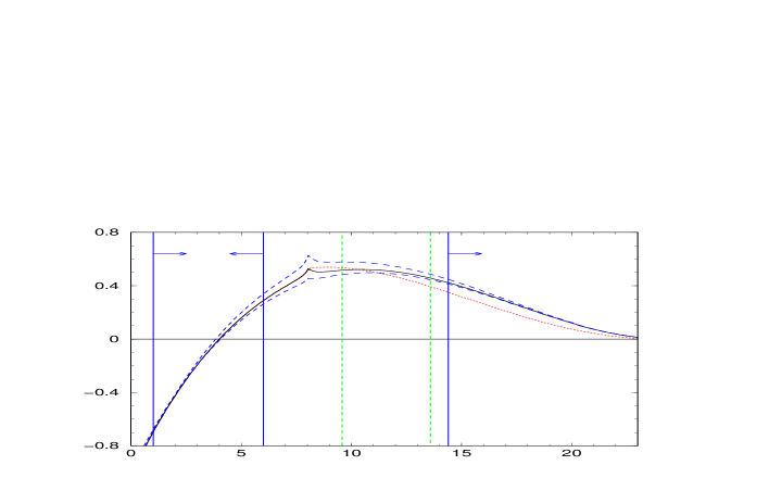
$\quad 10^{7}\times\displaystyle\frac{d{\cal A}_{\rm FB}}{dq^{2}}$ $\quad\ \ ({\rm GeV}^{-2})$
                                                                                                       $q^{2}~{}({\rm GeV}^{2})$

Figure 10: NNLL perturbative contributions to the un-normalized FB asymmetry; notations as in the upper plot of Fig. 8.

The summary plots for the lepton forward-backward asymmetry are shown in Fig. 10 and 11. In Fig. 10 we plot the un-normalized differential asymmetry, defined by

$$\frac{d{\cal A}_{\rm FB}(q^{2})}{dq^{2}} = \int_{-1}^{1}d\cos\theta_{\ell}~{}\frac{d^{2}{\cal B}(B\to X_{s}\ell^{+}\ell^{-})}{dq^{2}~{}d\cos\theta_{\ell}}\mbox{sgn}(\cos\theta_{\ell})$$ (6.39)

$$= \frac{{\cal B}(B\to X_{c}e\bar{\nu})}{m_{b}^{2}}A_{\rm FB}\left(\frac{q^{2}}{m_{b}^{2}}\right)~{},$$

while in Fig. 11 we plot the (adimensional) normalized differential asymmetry, defined by

$$\bar{\cal A}_{\rm FB}(q^{2})=\frac{1}{d{\cal B}(B\to X_{s}\ell^{+}\ell^{-})/dq^{2}}\int_{-1}^{1}d\cos\theta_{\ell}~{}\frac{d^{2}{\cal B}(B\to X_{s}\ell^{+}\ell^{-})}{dq^{2}~{}d\cos\theta_{\ell}}\mbox{sgn}(\cos\theta_{\ell})~{}.$$ (6.40)

Most of the comments concerning the errors and the complementary of low- and high-$q^{2}$ windows discussed before holds also for the forward-backward asymmetry.

In the low-$q^{2}$ region the most interesting observable is not the integral of the asymmetry, which is very small due to the change of sign, but the position of the zero. As discussed by several authors (see e.g. Ref. [4, 20]), this is one of the most precise predictions (and one of the most interesting SM tests) in rare $B$ decays. Denoting by $q^{2}_{0}$ the position of the zero, and showing explicitly only the uncertainties and non-perturbative effects larger than 0.5%, we find at the NNLL order

$$q^{2}_{0}=0.161\times m_{b}^{2}\times\left[1+0.9\%\big{|}_{1/m_{b}^{2}}\pm 5\%\big{|}_{\rm NNNLL}\right]=(3.90\pm 0.25)~{}{\rm GeV^{2}}~{}.$$ (6.41)

As already pointed out in Ref. [4], in this case the $\mu$ dependence is accidentally small and does not provides a conservative estimate of higher-order QCD corrections. The $5\%$ error in (6.41) has been estimated comparing the result within the ordinary LL counting and within the modified perturbative ordering proposed in Ref. [6] (see Sect. 2.4). The central value, as well as all the other central values in this work, is obtained using the modified ordering of Ref. [6].

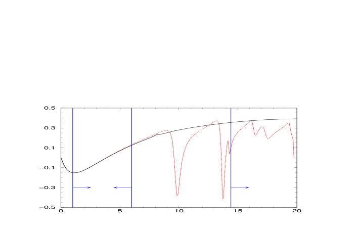
$\displaystyle\bar{\cal A}_{\rm FB}(q^{2})$
                                                                                                         $q^{2}~{}({\rm GeV}^{2})$

Figure 11: NNLL perturbative contributions to the normalized FB asymmetry; notations as in the lower plot of Fig. 8.

In the high-$q^{2}$ window the FB asymmetry does not change sign, therefore its integral represents an interesting observable. In order to minimize non-perturbative and normalization uncertainties it is more convenient to consider a normalized integrated asymmetry. Applying the same $q^{2}$ cut as in (6.34), we define

$$(\bar{\cal A}_{\rm FB})_{\rm cuts}^{\rm high}=\left[\int_{q^{2}>14.4~{}{\rm GeV}^{2}}dq^{2}~{}\frac{d{\cal B}_{\rm FB}(q^{2})}{dq^{2}}\right]^{-1}\int_{q^{2}>14.4~{}{\rm GeV}^{2}}dq^{2}~{}\frac{d{\cal A}_{\rm FB}(q^{2})}{dq^{2}}~{}.$$ (6.42)

All parametric and perturbative uncertainties are very small in this observable at the NNLL order level. On the other hand, despite a partial cancellation, this ratio is still affected by a considerable amount of $\Lambda^{2}_{\rm QCD}/m_{b}^{2}$ and $\Lambda^{3}_{\rm QCD}/m_{b}^{3}$ corrections (which represent the by-far dominant source of uncertainty). Taking into account the expressions in Sect. 5.2 and separating the contributions of the various operators, we find

$$(\bar{\cal A}_{\rm FB})_{\rm cuts}^{\rm high} = 0.42\times\left[1-(0.17\pm 0.11)_{\lambda_{1}}-(0.42\pm 0.07)_{\lambda_{2}}-(0.08\pm 0.08)_{\rho_{1}}\right]$$ (6.43)

$$= 0.14\pm 0.06~{}.$$

Appendix 1: Auxiliary functions

• The function $h(z)$ describing next-to-leading order QCD corrections to the semileptonic decay [see Eq. (2.2)] is given by [23]:

  $$h(z)= -(1-z^{2})\,\left(\frac{25}{4}-\frac{239}{3}\,z+\frac{25}{4}\,z^{2}\right)+z\,\ln(z)\left(20+90\,z-\frac{4}{3}\,z^{2}+\frac{17}{3}\,z^{3}\right)$$ (A.1)

  $$+z^{2}\,\ln^{2}(z)\,(36+z^{2})+(1-z^{2})\,\left(\frac{17}{3}-\frac{64}{3}\,z+\frac{17}{3}\,z^{2}\right)\,\ln(1-z)$$

  $$-4\,(1+30\,z^{2}+z^{4})\,\ln(z)\ln(1-z)-(1+16\,z^{2}+z^{4})\left(6\,\mbox{Li}(z)-\pi^{2}\right)$$

  $$-32\,z^{3/2}(1+z)\left[\pi^{2}-4\,\mbox{Li}(\sqrt{z})+4\,\mbox{Li}(-\sqrt{z})-2\ln(z)\,\ln\left(\frac{1-\sqrt{z}}{1+\sqrt{z}}\right)\right]~{}.$$

• In the counterterms to the two-loop matrix elements we use the following functions:

  $$B(a) = \int_{0}^{1}\ln(1-x(1-x)a)$$

  $$B_{x}(a) = \int_{0}^{1}x\ln(1-x(1-x)a)$$

  $$B_{xx}(a) = \int_{0}^{1}x^{2}\ln(1-x(1-x)a)$$

  $$B_{2}(a) = \int_{0}^{1}(\ln(1-x(1-x)a))^{2}$$

  $$B_{2x}(a) = \int_{0}^{1}x(\ln(1-x(1-x)a))^{2}$$

  $$B_{2xx}(a) = \int_{0}^{1}x^{2}(\ln(1-x(1-x)a))^{2}$$

  For the explicit expressions one should check $a=a+I\epsilon$ in order to remain on the correct Riemann sheet. Further functions are needed for the unexpanded counterterms:

  $$C(a) = \int_{0}^{1}2(x(1-x)a)/(1-x(1-x)a)$$

  $$C_{x}(a) = \int_{0}^{1}2x(x(1-x)a)/(1-x(1-x)a)$$

  $$C_{xx}(a) = \int_{0}^{1}2x^{2}(x(1-x)a)/(1-x(1-x)a)$$

  $$C_{2}(a) = \int_{0}^{1}4\ln(1-x(1-x)a)(x(1-x)a)/(1-x(1-x)a)$$

  $$C_{2x}(a) = \int_{0}^{1}4x\ln(1-x(1-x)a)(x(1-x)a)/(1-x(1-x)a)$$

  $$C_{2xx}(a) = \int_{0}^{1}4x^{2}\ln(1-x(1-x)a)(x(1-x)a)/(1-x(1-x)a)$$

Appendix 2: Effective Wilson coefficients

The effective coefficients $\widetilde{C}_{7-10}^{\rm eff}$ appearing in Eq. (2.7) are defined in our notation as,

$$\widetilde{C}_{7}^{\rm eff} = \frac{4\pi}{\alpha_{s}(\mu)}C_{7}(\mu)-\frac{1}{3}C_{3}(\mu)-\frac{4}{9}C_{4}(\mu)-\frac{20}{3}C_{5}(\mu)-\frac{80}{9}C_{6}(\mu)$$

$$\widetilde{C}_{8}^{\rm eff} = \frac{4\pi}{\alpha_{s}(\mu)}C_{8}(\mu)+C_{3}(\mu)-\frac{1}{6}C_{4}(\mu)+20C_{5}(\mu)-\frac{10}{3}C_{6}(\mu)$$

$$\widetilde{C}_{9}^{\rm eff}(s) = \frac{4\pi}{\alpha_{s}(\mu)}C_{9}(\mu)+\sum_{i=1}^{6}C_{i}(\mu)\gamma^{(0)}_{i9}\ln\left(\frac{m_{b}}{\mu}\right)$$

$$+ \frac{4}{3}C_{3}(\mu)+\frac{64}{9}C_{5}(\mu)+\frac{64}{27}C_{6}(\mu)$$

$$+ h\left(z,s\right)\left(\frac{4}{3}C_{1}(\mu)+C_{2}(\mu)+6C_{3}(\mu)+60C_{5}(\mu)\right)$$

$$+ h(1,s)\left(-\frac{7}{2}C_{3}(\mu)-\frac{2}{3}C_{4}(\mu)-38C_{5}(\mu)-\frac{32}{3}C_{6}(\mu)\right)$$

$$+ h(0,s)\left(-\frac{1}{2}C_{3}(\mu)-\frac{2}{3}C_{4}(\mu)-8C_{5}(\mu)-\frac{32}{3}C_{6}(\mu)\right)$$

$$\equiv A_{9}+h(z,s)T_{9}+h(1,s)U_{9}+h(0,s)W_{9}$$

$$\widetilde{C}_{10}^{\rm eff} = \frac{4\pi}{\alpha_{s}(\mu)}C_{10}(\mu)~{},$$ (A.4)

where

$$h(z,s) = -\frac{4}{9}\ln(z)+\frac{8}{27}+\frac{16}{9}\frac{z}{s}-\frac{2}{9}\left(2+\frac{4\,z}{s}\right)\sqrt{\left|\frac{4\,z-s}{s}\right|}\times$$ (A.7)

$$\times \left\{\begin{array}[]{ll}2\arctan\sqrt{\frac{s}{4\,z-s}}&\mbox{for}\,s<4\,z\,,\\ \ln\left(\frac{\sqrt{s}+\sqrt{s-4\,z}}{\sqrt{s}-\sqrt{s-4\,z}}\right)-i\,\pi&\mbox{for}\,s>4\,z\,.\end{array}\right.$$

Note that specific one- and two-loop and matrix-element contributions of the four-quark operators ${\cal O}_{1-6}$ (including the corresponding bremsstrahlung contributions) such as the one shown in Fig. A1 are included by the redefinition of the Wilson coefficients $C_{7}$, $C_{9}$ and $C_{10}$ given in (A.4). In fact, using this redefinition, the bremsstrahlung and virtual corrections that are shown in Fig. A2 (see next subsection) automatically take these effects into account. The Wilson coefficients $C_{i}$ in (A.4), which are needed to NNLL precision, are presented in [17, 6]. For completeness we quote them here again:

	$\mu=2.5$ GeV	$\mu=5$ GeV	$\mu=10$ GeV
$\alpha_{s}$	$0.267$	$0.215$	$0.180$
$C_{1}^{(0)}$	$-0.697$	$-0.487$	$-0.326$
$C_{2}^{(0)}$	$1.046$	$1.024$	$1.011$
$\big{(}\widetilde{C}_{7}^{{\rm eff}\,(0)},~{}\widetilde{C}_{7}^{{\rm eff}\,(1)}\big{)}$	$(-0.360,~{}0.031)$	$(-0.321,~{}0.019)$	$(-0.287,~{}0.008)$
$\widetilde{C}_{8}^{{\rm eff}\,(0)}$	$-0.164$	$-0.148$	$-0.134$
$\big{(}A_{9}^{(0)},~{}A_{9}^{(1)}\big{)}$	$(4.241,~{}-0.170)$	$(4.129,~{}0.013)$	$(4.131,~{}0.155)$
$\big{(}T_{9}^{((0))},~{}T_{9}^{(1)}\big{)}$	$(0.115,~{}0.278)$	$(0.374,~{}0.251)$	$(0.576,~{}0.231)$
$\big{(}U_{9}^{(0)},~{}U_{9}^{(1)}\big{)}$	$(0.045,~{}0.023)$	$(0.032,~{}0.016)$	$(0.022,~{}0.011)$
$\big{(}W_{9}^{(0)},~{}W_{9}^{(1)}\big{)}$	$(0.044,~{}0.016)$	$(0.032,~{}0.012)$	$(0.022,~{}0.009)$
$\big{(}\widetilde{C}_{10}^{{\rm eff}\,(0)},~{}\widetilde{C}_{10}^{{\rm eff}\,(1)}\big{)}$	$(-4.372,~{}0.135)$	$(-4.372,~{}0.135)$	$(-4.372,~{}0.135)$

Table 3: Numerical values of Wilson coefficients of (A.4) for three different values of $\mu$; the $\alpha_{s}$ expansion of the terms are defined by $C_{i}^{\rm eff}=C_{i}^{{\rm eff}\,(0)}+C_{i}^{{\rm eff}\,(1)}+...$  .

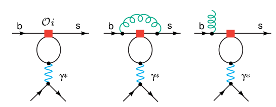
Figure A1: Examples of virtual and bremsstrahlung contributions of the four-quark operators ${\cal O}_{1\ldots 6}$ that are taken into account by the redefinition of the Wilson coefficients in Eq. (A.4).

Appendix 3: IR virtual and bremsstrahlung corrections

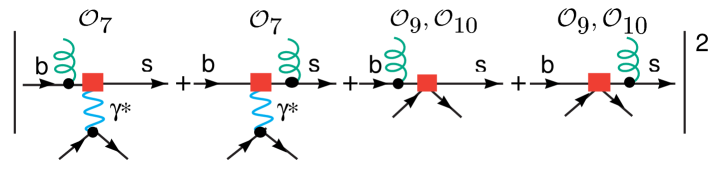
Figure A2: Virtual (up) and real (down) QCD corrections generating the terms $\tau_{i}$ and $\sigma_{i}$.

The universal $O(\alpha_{s})$ bremsstrahlung and the corresponding infrared (IR) virtual corrections which can be absorbed into the Wilson coefficients (see (2.7)) were calculated in [19, 4, 20] and given by

$$\sigma_{9}(s) = \sigma(s)+\frac{3}{2}~{},\qquad\qquad\sigma_{7}(s)\ =\ \sigma(s)+\frac{1}{6}-\frac{8}{3}\ln\left(\frac{\mu}{m_{b}}\right)~{},$$

$$\sigma(s) = -\frac{4}{3}\mbox{Li}_{2}(s)-\frac{2}{3}\ln(s)\ln(1-s)-\frac{2}{9}\pi^{2}-\ln(1-s)-\frac{2}{9}(1-s)\ln(1-s)~{}.\qquad$$ (A.8)

The remaining (finite) non-universal bremsstrahlung are encoded in rate (see 2.5)) and FB asymmetry (see 2.6)). We note that we have chosen the universal functions $\sigma_{i}$ in (A.8) such that the non-universal contributions to the rate, namely $\tau_{77},\tau_{99},\tau_{79}$, vanish in the limit $s\rightarrow 1$:

$$\tau_{77}(s) = -\frac{2}{9(2+s)}\left[2(1-s)^{2}\ln(1-s)+\frac{6s(2-2s-s^{2})}{(1-s)^{2}}\ln(s)+\frac{11-7s-10s^{2}}{(1-s)}\right]~{},$$

$$\tau_{99}(s) = -\frac{4}{9(1+2s)}\left[2(1-s)^{2}\ln(1-s)+\frac{3s(1+s)(1-2s)}{(1-s)^{2}}\ln(s)+\frac{3(1-3s^{2})}{1-s}\right]~{},$$

$$\tau_{79}(s) = -\frac{4(1-s)^{2}}{9s}\ln(1-s)-\frac{4s(3-2s)}{9(1-s)^{2}}\ln(s)-\frac{2(5-3s)}{9(1-s)}~{},$$ (A.9)

$$\tau_{710}(s) = -\frac{5}{2}+\frac{1}{3(1-3s)}-\frac{1}{3}\frac{s(6-7s)\ln(s)}{(1-s)^{2}}-\frac{1}{9}\frac{(3-7s+4s^{2})\ln(1-s)}{s}+\frac{f_{7}(s)}{3}$$

$$\tau_{910}(s) = -\frac{5}{2}+\frac{1}{3(1-s)}-\frac{1}{3}\frac{s(6-7s)\ln(s)}{((1-s)^{2})}-\frac{2}{9}\frac{(3-5s+2s^{2})\ln(1-s)}{s}+\frac{f_{9}(s)}{3}$$ (A.10)

where

$$f_{7}(s) = \frac{1}{6(s-1)^{2}}\Big{\{}24(1+13s-4s^{2}){\rm Li}_{2}(\sqrt{s})+12(1-17s+6s^{2}){\rm Li}_{2}(s)+6s(6-7s)\ln(s)$$ (A.11)

$$+24(1-s)^{2}\ln(s)\ln(1-s)+12(-13+16s-3s^{2})[\ln(1-\sqrt{s})-\ln(1-s)]$$

$$+39-2\pi^{2}+252s-26\pi^{2}s+21s^{2}+8\pi^{2}s^{2}-180\sqrt{s}-132s\sqrt{s}\Big{\}}~{},$$

$$f_{9}(s) = -\frac{1}{6(s-1)^{2}}\Big{\{}48s(-5+2s){\rm Li}_{2}(\sqrt{s})+24(-1+7s-3s^{2}){\rm Li_{2}}(s)+6s(-6+7s)\ln(s)$$ (A.12)

$$-24(1-s)^{2}\ln(s)\ln(1-s)+24(5-7s+2s^{2})[\ln(1-\sqrt{s})-\ln(1-s)]$$

$$-21-156s+20\pi^{2}s+9s^{2}-8\pi^{2}s^{2}+120\sqrt{s}+48s\sqrt{s}\Big{\}}~{}.$$

Appendix 4: Complete set of scalar integrals

In [26] it was shown that there are ten linear combinations of the integrals

$$\tilde{\cal P}^{a\,b}_{\alpha_{1}\,\alpha_{2}\,\alpha_{3}}(m_{1},m_{2},m_{3};k^{2})=\int d^{n}p\,d^{n}q\,\frac{(p\cdot k)^{a}(q\cdot k)^{b}}{[(p+k)^{2}+m_{1}^{2}]^{\alpha_{1}}\,(q^{2}+m_{2}^{2})^{\alpha_{2}}\,(r^{2}+m_{3}^{2})^{\alpha_{3}}\,,}$$ (A.13)

with $a+b\leq 3$, which are sufficient for treating all two-loop Feynman diagrams which one can encounter in renormalizable theories. Because the ultravilet behaviour of the functions ${\cal H}_{i}$ is logarithmic only, one finds simple finite integral representations:

$${\cal H}_{1} = \pi^{4}\left[\frac{1}{2\epsilon^{2}}+\frac{1}{2\epsilon}(1-2\gamma_{m_{1}})-\frac{1}{2}+\frac{\pi^{2}}{12}-\gamma_{m_{1}}+\gamma_{m_{1}}^{2}+h_{1}\right]$$

$${\cal H}_{2} = \pi^{4}k^{2}\left[-\frac{1}{2\epsilon^{2}}-\frac{1}{2\epsilon}(\frac{1}{2}-2\gamma_{m_{1}})+\frac{13}{8}-\frac{\pi^{2}}{12}+\frac{\gamma_{m_{1}}}{2}-\gamma_{m_{1}}^{2}-h_{2}\right]$$

$${\cal H}_{3} = \pi^{4}k^{2}\left[\frac{1}{4\epsilon^{2}}+\frac{1}{2\epsilon}(\frac{1}{4}-\gamma_{m_{1}})-\frac{13}{16}+\frac{\pi^{2}}{24}-\frac{\gamma_{m_{1}}}{4}+\frac{\gamma_{m_{1}}^{2}}{2}+h_{3}\right]$$

$${\cal H}_{4} = \pi^{4}(k^{2})^{2}\left[\frac{3}{8\epsilon^{2}}-\frac{1}{2\epsilon}\frac{3\gamma_{m_{1}}}{2}-\frac{175}{96}+\frac{\pi^{2}}{16}+\frac{3\gamma_{m_{1}}^{2}}{4}+\frac{3}{4}h_{4}\right]$$

$${\cal H}_{5} = \pi^{4}(k^{2})^{2}\left[-\frac{3}{16\epsilon^{2}}+\frac{1}{2\epsilon}\frac{3\gamma_{m_{1}}}{4}+\frac{175}{192}-\frac{\pi^{2}}{32}-\frac{3\gamma_{m_{1}}^{2}}{8}-\frac{3}{4}h_{5}\right]$$

$${\cal H}_{6} = \pi^{4}(k^{2})^{2}\left[\frac{1}{8\epsilon^{2}}+\frac{1}{2\epsilon}(\frac{1}{24}-\frac{\gamma_{m_{1}}}{2})-\frac{19}{32}+\frac{\pi^{2}}{48}-\frac{\gamma_{m_{1}}}{24}+\frac{\gamma_{m_{1}}^{2}}{4}+\frac{3}{4}h_{6}\right]$$

$${\cal H}_{7} = \pi^{4}(k^{2})^{3}\left[-\frac{1}{4\epsilon^{2}}+\frac{1}{2\epsilon}(\frac{5}{24}+\gamma_{m_{1}})+\frac{287}{192}-\frac{\pi^{2}}{24}-\frac{5\gamma_{m_{1}}}{24}-\frac{\gamma_{m_{1}}^{2}}{2}-\frac{1}{2}h_{7}\right]$$

$${\cal H}_{8} = \pi^{4}(k^{2})^{3}\left[\frac{1}{8\epsilon^{2}}-\frac{1}{2\epsilon}(\frac{5}{48}+\frac{\gamma_{m_{1}}}{2})-\frac{287}{384}+\frac{\pi^{2}}{48}+\frac{5\gamma_{m_{1}}}{48}+\frac{\gamma_{m_{1}}^{2}}{4}+\frac{1}{2}h_{8}\right]$$

$${\cal H}_{9} = \pi^{4}(k^{2})^{3}\left[-\frac{1}{12\epsilon^{2}}+\frac{1}{2\epsilon}(\frac{1}{24}+\frac{\gamma_{m_{1}}}{3})+\frac{95}{192}-\frac{\pi^{2}}{72}-\frac{\gamma_{m_{1}}}{24}-\frac{\gamma_{m_{1}}^{2}}{6}-\frac{1}{2}h_{9}\right]$$

$${\cal H}_{10} = \pi^{4}(k^{2})^{3}\left[\frac{1}{16\epsilon^{2}}-\frac{1}{2\epsilon}(\frac{1}{96}+\frac{\gamma_{m_{1}}}{4})-\frac{283}{768}+\frac{\pi^{2}}{96}+\frac{\gamma_{m_{1}}}{96}+\frac{\gamma_{m_{1}}^{2}}{8}+\frac{1}{2}h_{10}\right]\;\;.$$ (A.14)

$d=4-2\epsilon$ is the space-time dimension, and $\gamma_{m}=\gamma+\log(\pi m^{2}/\mu_{1}^{2})$. The special functions $h_{i}$ which appear in the formulae above are the finite part in the $1/\epsilon$ expansion of ${\cal H}_{i}$ and cannot be further integrated into well-studied functions, such as the familiar polylogarithms:

$$h_{1}(m_{1},m_{2},m_{3};k^{2}) = \int_{0}^{1}dx\,\tilde{g}(x)$$

$$h_{2}(m_{1},m_{2},m_{3};k^{2}) = \int_{0}^{1}dx\,[\tilde{g}(x)+\tilde{f_{1}}(x)]$$

$$h_{3}(m_{1},m_{2},m_{3};k^{2}) = \int_{0}^{1}dx\,[\tilde{g}(x)+\tilde{f_{1}}(x)]\,(1-x)$$

$$h_{4}(m_{1},m_{2},m_{3};k^{2}) = \int_{0}^{1}dx\,[\tilde{g}(x)+\tilde{f_{1}}(x)+\tilde{f_{2}}(x)]$$

$$h_{5}(m_{1},m_{2},m_{3};k^{2}) = \int_{0}^{1}dx\,[\tilde{g}(x)+\tilde{f_{1}}(x)+\tilde{f_{2}}(x)]\,(1-x)$$

$$h_{6}(m_{1},m_{2},m_{3};k^{2}) = \int_{0}^{1}dx\,[\tilde{g}(x)+\tilde{f_{1}}(x)+\tilde{f_{2}}(x)]\,(1-x)^{2}$$

$$h_{7}(m_{1},m_{2},m_{3};k^{2}) = \int_{0}^{1}dx\,[\tilde{g}(x)+\tilde{f_{1}}(x)+\tilde{f_{2}}(x)+\tilde{f_{3}}(x)]$$

$$h_{8}(m_{1},m_{2},m_{3};k^{2}) = \int_{0}^{1}dx\,[\tilde{g}(x)+\tilde{f_{1}}(x)+\tilde{f_{2}}(x)+\tilde{f_{3}}(x)]\,(1-x)$$

$$h_{9}(m_{1},m_{2},m_{3};k^{2}) = \int_{0}^{1}dx\,[\tilde{g}(x)+\tilde{f_{1}}(x)+\tilde{f_{2}}(x)+\tilde{f_{3}}(x)]\,(1-x)^{2}$$

$$h_{10}(m_{1},m_{2},m_{3};k^{2}) = \int_{0}^{1}dx\,[\tilde{g}(x)+\tilde{f_{1}}(x)+\tilde{f_{2}}(x)+\tilde{f_{3}}(x)]\,(1-x)^{3}\;\;.$$ (A.15)

The four building blocks $\tilde{g}(x)$, $\tilde{f_{1}}(x)$, $\tilde{f_{2}}(x)$, and $\tilde{f_{3}}(x)$ of these one-dimensional integral representations are explicitly given in section 3.2.

Appendix 5: Anomalous dimensions

We quote here all anomalous dimensions necessary for the calculation. They were presented in [17, 18] and have been checked by us.

The counterterm contribution which are proportional to $C_{1}$ and $C_{2}$ due to the mixing of the two operators ${\cal O}_{1}$ and ${\cal O}_{2}$ with the operators ${\cal O}_{j}\quad(j=1...12)$ are given by the following matrix elements

$$\langle s\ell^{+}\ell^{-}|\,\sum_{j=1}^{12}\delta Z_{ij}O_{j}\,|b\rangle\,,\quad i=1,2,$$ (A.16)

with the renormalization constants $Z_{ij}=\delta_{ij}+\delta Z_{ij}$ where

$$\delta Z_{ij}=\frac{\alpha_{s}}{4\pi}\left(a_{ij}^{01}+\frac{1}{\epsilon}a_{ij}^{11}\right)+\frac{\alpha_{s}^{2}}{(4\pi)^{2}}\left(a_{ij}^{02}+\frac{1}{\epsilon}a_{ij}^{12}+\frac{1}{\epsilon^{2}}a_{ij}^{22}\right)+O(\alpha_{s}^{3}).$$ (A.17)

There are two evanescent operators ${\cal O}_{11}$ and ${\cal O}_{12}$ involved in the mixing in addition to the operator basis given in (2.3). As usual, their choice is not unique, but we follow the ones used by the authors of [17] so as to be able to use their results for the Wilson coefficients:

$${\cal O}_{11} = ({\bar{s}}_{L}\gamma_{\mu}\gamma_{\nu}\gamma_{\sigma}T^{a}c_{L})({\bar{c}}_{L}\gamma^{\mu}\gamma^{\nu}\gamma^{\sigma}T^{a}b_{L})-16\,\,{\cal O}_{1}\,,$$

$${\cal O}_{12} = ({\bar{s}}_{L}\gamma_{\mu}\gamma_{\nu}\gamma_{\sigma}c_{L})({\bar{c}}_{L}\gamma^{\mu}\gamma^{\nu}\gamma^{\sigma}b_{L})-16\,\,{\cal O}_{2}\,.$$ (A.18)

The anomalous dimensions are given then by:

$a^{11}_{ij}$	j=1	j=2	j=3	j=4	j=5	j=6	j=7	j=8	j=9	j=10	j=11	j=12
i=1	-2	4/3	0	-1/9	0	0	0	0	-16/27	0	5/12	2/9
i=2	6	0	0	2/3	0	0	0	0	-4/9	0	1	0

$a^{22}_{ij}$	j=1	j=2	j=3	j=4	j=5	j=6	j=7	j=8	j=9	j=10	j=11	j=12
i=1	*	*	*	*	*	*	*	*	1168/243	*	*	*
i=2	*	*	*	*	*	*	*	*	148/81	*	*	*

$a^{12}_{ij}$	j=1	j=2	j=3	j=4	j=5	j=6	j=7	j=8	j=9	j=10	j=11	j=12
i=1	*	*	*	*	*	*	-58/243	*	-64/729	*	*	*
i=2	*	*	*	*	*	*	116/81	*	776/243	*	*	*

Appendix 6: $O(\Lambda^{2}_{\rm QCD}/m_{c}^{2})$ corrections.

The explicit expressions of the $O(\Lambda^{2}_{\rm QCD}/m_{c}^{2})$ non-factorizable corrections to $R(s)$ and $A_{\rm FB}$ are [36]:

$$\delta_{1/m^{2}_{c}}R(s) = \frac{8\lambda_{2}}{9m^{2}_{c}}\frac{\alpha_{\rm em}^{2}}{4\pi^{2}}\frac{V_{cs}^{*}V_{ts}}{V_{cb}^{*}V_{tb}}\frac{(1-s)^{2}}{f(z)\kappa(z)}\ \mbox{Re}\Biggl{[}\frac{1+6s-s^{2}}{s}F\left(\frac{s}{4z}\right)C_{2}C^{\rm new}_{7}(s)^{*}$$ (A.19)

$$\qquad\qquad\qquad\qquad\qquad\qquad\quad+(2+s)F\left(\frac{s}{4z}\right)C_{2}C^{\rm new}_{9}(s)^{*}\Biggl{]}~{},$$

$$\delta_{1/m^{2}_{c}}A(s) = -\frac{\lambda_{2}}{3m^{2}_{c}}\frac{\alpha_{\rm em}^{2}}{4\pi^{2}}\frac{V_{cs}^{*}V_{ts}}{V_{cb}^{*}V_{tb}}\frac{(1-s)^{2}}{f(z)\kappa(z)}\ \mbox{Re}\Biggl{[}(1+3s)F\left(\frac{s}{4z}\right)C_{2}C^{\rm new}_{10}(s)^{*}\Biggl{]}~{},$$ (A.20)

where

$$F(r)=\frac{3}{2r}\left\{\begin{array}[]{ll}\displaystyle\frac{1}{\sqrt{r(1-r)}}\arctan\sqrt{\frac{r}{1-r}}-1&\qquad\qquad 0<r<1~{},\\ \displaystyle\frac{1}{2\sqrt{r(r-1)}}\left(\ln\frac{1-\sqrt{1-1/r}}{1+\sqrt{1-1/r}}+i\pi\right)-1&\qquad\qquad r>1~{}.\end{array}\right.$$ (A.21)

References

- [1] G. D’Ambrosio, G. F. Giudice, G. Isidori and A. Strumia, Nucl. Phys. B 645 (2002) 155 [hep-ph/0207036]; G. Degrassi, P. Gambino and G. F. Giudice, JHEP 0012 (2000) 009 [hep-ph/0009337]; M. Carena, D. Garcia, U. Nierste and C. E. Wagner, Phys. Lett. B 499 (2001) 141 [hep-ph/0010003].
- [2] F. Borzumati, C. Greub, T. Hurth and D. Wyler, Phys. Rev. D 62 (2000) 075005 [hep-ph/9911245]; T. Besmer, C. Greub and T. Hurth, Nucl. Phys. B 609 (2001) 359 [hep-ph/0105292].
- [3] T. Hurth, Rev. Mod. Phys. 75 (2003) 1159 [hep-ph/0212304]; hep-ph/0106050.
- [4] A. Ghinculov, T. Hurth, G. Isidori and Y. P. Yao, Nucl. Phys. B 648 (2003) 254 [hep-ph/0208088].
- [5] A. Ghinculov, T. Hurth, G. Isidori and Y. P. Yao, Nucl. Phys. Proc. Suppl. 116 (2003) 284 [hep-ph/0211197]; hep-ph/0310187.
- [6] H. H. Asatrian, H. M. Asatrian, C. Greub and M. Walker, Phys. Lett. B 507 (2001) 162 [hep-ph/0103087]; H. H. Asatrian, H. M. Asatrian, C. Greub and M. Walker, Phys. Rev. D 65 (2002) 074004 [hep-ph/0109140].
- [7] J. Kaneko et al. [Belle Collaboration], Phys. Rev. Lett. 90 (2003) 021801 [hep-ex/0208029].
- [8] B. Aubert et al. [BABAR Collaboration], hep-ex/0308016.
- [9] A. Ali and E. Pietarinen, Nucl. Phys. B 154 (1979) 519; G. Altarelli, N. Cabibbo, G. Corbo, L. Maiani and G. Martinelli, Nucl. Phys. B 208 (1982) 365.
- [10] M. Misiak, Nucl. Phys. B 393 (1993) 23; ibid. 439 (1993) 461 (E).
- [11] A. J. Buras and M. Munz, Phys. Rev. D 52 (1995) 186 [hep-ph/9501281].
- [12] K. Adel and Y. Yao, Phys. Rev. D 49 (1994) 4945 [hep-ph/9308349].
- [13] C. Greub and T. Hurth, Phys. Rev. D 56 (1997) 2934 [hep-ph/9703349].
- [14] K. Chetyrkin, M. Misiak and M. Munz, Phys. Lett. B 400 (1997) 206 [hep-ph/9612313].
- [15] C. Greub, T. Hurth and D. Wyler, Phys. Lett. B 380 (1996) 385 [hep-ph/9602281]; Phys. Rev. D 54 (1996) 3350 [hep-ph/9603404].
- [16] A. J. Buras, A. Czarnecki, M. Misiak and J. Urban, Nucl. Phys. B 611 (2001) 488 [hep-ph/0105160].
- [17] C. Bobeth, M. Misiak and J. Urban, Nucl. Phys. B 574 (2000) 291 [hep-ph/9910220].
- [18] P. Gambino, M. Gorbahn and U. Haisch, hep-ph/0306079.
- [19] H. H. Asatryan, H. M. Asatrian, C. Greub and M. Walker, Phys. Rev. D 66, 034009 (2002).
- [20] H. M. Asatrian, K. Bieri, C. Greub and A. Hovhannisyan, Phys. Rev. D 66 (2002) 094013 [hep-ph/0209006]
- [21] H. M. Asatrian, H. H. Asatryan, A. Hovhannisyan and V. Poghosyan, hep-ph/0311187.
- [22] A. J. Buras, A. Czarnecki, M. Misiak and J. Urban, Nucl. Phys. B 631, 219 (2002) [hep-ph/0203135].
- [23] Y. Nir, Phys. Lett. B 221 (1989) 184.
- [24] A. Ali, G. Hiller, L. T. Handoko and T. Morozumi, Phys. Rev. D 55 (1997) 4105 [hep-ph/9609449].
- [25] P. L. Cho, M. Misiak and D. Wyler, Phys. Rev. D 54 (1996) 3329 [hep-ph/9601360].
- [26] A. Ghinculov and Y. P. Yao, Phys. Rev. D 63 (2001) 054510 [hep-ph/0006314].
- [27] G. Buchalla and G. Isidori, Nucl. Phys. B 525 (1998) 333 [hep-ph/9801456].
- [28] See e.g. M. Neubert, Phys. Rep. 245 (1994) 259 [hep-ph/9306320].
- [29] A. F. Falk, B. Grinstein and M. E. Luke, Nucl. Phys. B 357 (1991) 185.
- [30] M. Neubert, JHEP 0007 (2000) 022 [arXiv:hep-ph/0006068].
- [31] C. W. Bauer and C. N. Burrell, Phys. Lett. B 469 (1999) 248 [hep-ph/9907517]; Phys. Rev. D 62 (2000) 114028 [hep-ph/9911404].
- [32] M. Gremm and A. Kapustin, Phys. Rev. D 55 (1997) 6924 [hep-ph/9603448].
- [33] M. Battaglia et al., The CKM matrix and the unitarity triangle, hep-ph/0304132.
- [34] F. Krüger and L.M. Sehgal, Phys. Lett. B 380 (1996) 199 [hep-ph/9603237].
- [35] G. Hiller, private communication.
- [36] G. Buchalla, G. Isidori and S. J. Rey, Nucl. Phys. B 511 (1998) 594 [hep-ph/9705253].
- [37] J. W. Chen, G. Rupak and M. J. Savage, Phys. Lett. B 410 (1997) 285 [hep-ph/9705219].
- [38] M.B. Voloshin, Phys. Lett. B 397 (1997) 275 [hep-ph/9612483]; A. Khodjamirian, R. Ruckl, G. Stoll and D. Wyler, Phys. Lett. B 402 (1997) 167 [hep-ph/9702318].
- [39] P. Gambino and M. Misiak, Nucl. Phys. B 611 (2001) 338 [hep-ph/0104034].
- [40] A. Ali, E. Lunghi, C. Greub and G. Hiller, Phys. Rev. D 66 (2002) 034002 [hep-ph/0112300].
- [41] M. Nakao, hep-ex/0312041.
- [42] Heavy Flavor Averaging Group, data available at http://www.slac.stanford.edu/xorg/hfag/
- [43] C. Bobeth, P. Gambino, M. Gorbahn and U. Haisch, hep-ph/0312090.