Probing Neutrino Parameters at Accelerators

Abstract:

The simplest unified extension of the Minimal Supersymmetric Standard Model with bilinear R–Parity violation provides a predictive scheme for neutrino masses and mixings which can account for the observed atmospheric and solar neutrino anomalies. Despite the smallness of neutrino masses R-parity violation is observable at present and future high-energy colliders, providing an unambiguous cross-check of the model.

1 Introduction

The announcement of high statistics atmospheric neutrino data by the SuperKamiokande collaboration [1] has confirmed the deficit of muon neutrinos, especially at small zenith angles, opening a new era in neutrino physics. Although in the past have been considered alternative solutions for the atmospheric neutrino anomaly  [2, 3] it is now clear that the simplest interpretation of the data is in terms of $\nu_{\mu}$ to $\nu_{\tau}$ flavor oscillations with maximal mixing. This excludes a large mixing among $\nu_{\tau}$ and $\nu_{e}$ [1], in agreement also with the CHOOZ reactor data [4, 5]. On the other hand, the persistent disagreement between solar neutrino data [6] and theoretical expectations [7] has been a long-standing problem in physics. Recent solar neutrino data from the Kamland collaboration [8] and the latest results from the SNO collaboration [9], clearly indicate that we have MSW conversions with a large mixing angle  [10]. For the solar neutrino parameters we get for the best fit point [10]:

$$\tan^{2}\theta{sol}=0.43,\qquad\Delta m^{2}{sol}=6.9\times 10^{-5}~{}\rm{eV}^{2}\,,$$ (1)

confirming that the solar neutrino mixing angle is large, but significantly non-maximal. The $3\sigma$ region for $\theta$ is:

$$0.30\leq\tan^{2}\theta{sol}\leq 0.64,$$ (2)

while the $3\sigma$ region for $\Delta m^{2}{sol}$ range is given by,

$$5.4\times 10^{-5}~{}\rm{eV}^{2}\leq\Delta m^{2}{sol}\leq 9.5\times 10^{-5}~{}\rm{eV}^{2},$$ (3)

On the other hand, current atmospheric neutrino data require oscillations involving $\nu_{\mu}\leftrightarrow\nu_{\tau}$  [1]. The most recent global analysis gives [10],

$$\sin^{2}\theta{atm}=0.52\,,\>\Delta m^{2}{atm}=2.6\times 10^{-3}~{}\rm{eV}^{2}\>$$ (4)

with the 3$\sigma$ ranges,

$$0.31\leq\sin^{2}\theta{atm}\leq 0.72$$ (5)

$$1.4\times 10^{-3}~{}\rm{eV}^{2}\leq\Delta m^{2}{atm}\leq 3.7\times 10^{-3}~{}\rm{eV}^{2}\,.$$ (6)

Many attempts have appeared in the literature to explain the data. Here we review recent results [11, 12, 13, 14, 15, 16] obtained in a model [17] which is a simple extension of the Minimal Supersymmetric Standard Model (MSSM) with bilinear R-parity violation (BRpV). This model, despite being a minimal extension of the MSSM, can explain the solar and atmospheric neutrino data. Its most attractive feature is that it gives definite predictions for accelerator physics for the same range of parameters that explain the neutrino data.

2 The Model

Since BRpV has been discussed in the literature several times [11, 12, 17, 18, 19, 20] we will repeat only the main features of the model here. We will follow the notation of [11, 12]. The simplest bilinear $R_{p}/\;\>$ model (we call it the $R_{p}/\;\>$ MSSM) is characterized by the superpotential

$$W=W_{MSSM}+W_{R\!\!\!/_{P}}$$ (7)

In this equation $W_{MSSM}$ is the ordinary superpotential of the MSSM,

$$W=\varepsilon_{ab}\left[h_{U}^{ij}\widehat{Q}_{i}^{a}\widehat{U}_{j}\widehat{H}_{u}^{b}+h_{D}^{ij}\widehat{Q}_{i}^{b}\widehat{D}_{j}\widehat{H}_{d}^{a}+h_{E}^{ij}\widehat{L}_{i}^{b}\widehat{R}_{j}\widehat{H}_{d}^{a}-\mu\widehat{H}_{d}^{a}\widehat{H}_{u}^{b}\right]$$ (8)

where $i,j=1,2,3$ are generation indices, $a,b=1,2$ are $SU(2)$ indices. We have three additional terms that break R-parity,

$$W_{R\!\!\!/_{P}}=\epsilon_{ab}\epsilon_{i}\widehat{L}^{a}_{i}\widehat{H}^{b}_{u}.$$ (9)

These bilinear terms, together with the corresponding terms in the soft supersymmetric (SUSY) breaking part of the Lagrangian,

$$V_{soft}=V_{soft}^{MSSM}+\epsilon_{ab}B_{i}\epsilon_{i}{\tilde{L}}^{a}_{i}H^{b}_{u}$$ (10)

define the minimal model, which we will adopt throughout this paper. The appearance of the lepton number violating terms in Eq. (9) leads in general to non-zero vacuum expectation values for the scalar neutrinos $\langle{\tilde{\nu}}_{i}\rangle$, called $v_{i}$ in the rest of this paper, in addition to the VEVs $v_{U}$ and $v_{D}$ of the MSSM Higgs fields $H_{u}^{0}$ and $H_{d}^{0}$. Together with the bilinear parameters $\epsilon_{i}$ the $v_{i}$ induce mixing between various particles which in the MSSM are distinguished (only) by lepton number (or R–parity). Mixing between the neutrinos and the neutralinos of the MSSM generates a non-zero mass for one specific linear superposition of the three neutrino flavor states of the model at tree-level while 1-loop corrections provide mass for the remaining two neutrino states [11, 12].

3 Neutrino Masses and Mixings

3.1 Tree Level Neutral Fermion Mass Matrix

In the basis $\psi^{0T}=(-i\lambda^{\prime},-i\lambda^{3},\widetilde{H}_{d}^{1},\widetilde{H}_{u}^{2},\nu_{e},\nu_{\mu},\nu_{\tau})$ the neutral fermions mass terms in the Lagrangian are given by

$$\mathcal{L}_{m}=-\frac{1}{2}(\psi^{0})^{T}{\kern-0.24994pt\hbox{$M$}\kern-10.79166pt\kern 0.50003pt\hbox{$M$}\kern-10.79166pt\kern-0.24994pt\raise 0.43304pt\hbox{$M$}}_{N}\psi^{0}+h.c.$$ (11)

where the neutralino/neutrino mass matrix is

$${\kern-0.24994pt\hbox{$M$}\kern-10.79166pt\kern 0.50003pt\hbox{$M$}\kern-10.79166pt\kern-0.24994pt\raise 0.43304pt\hbox{$M$}}_{N}=\left[\begin{array}[]{cc}\mathcal{M}_{\chi^{0}}&m^{T}\cr m&0\cr\end{array}\right]$$ (12)

with

$$\mathcal{M}_{\chi^{0}}=\left[\begin{array}[]{cccc}M_{1}&0&-\frac{1}{2}g^{\prime}v_{d}&\frac{1}{2}g^{\prime}v_{u}\cr 0&M_{2}&\frac{1}{2}gv_{d}&-\frac{1}{2}gv_{u}\cr-\frac{1}{2}g^{\prime}v_{d}&\frac{1}{2}gv_{d}&0&-\mu\cr\frac{1}{2}g^{\prime}v_{u}&-\frac{1}{2}gv_{u}&-\mu&0\cr\end{array}\right]\quad;\quad m=\left[\begin{array}[]{c}a_{1}\cr a_{2}\cr a_{3}\end{array}\right]$$ (13)

where $a_{i}=(-\frac{1}{2}g^{\prime}v_{i},\frac{1}{2}gv_{i},0,\epsilon_{i})$. This neutralino/neutrino mass matrix is diagonalized by

$$\mathcal{N}^{*}{\kern-0.24994pt\hbox{$M$}\kern-10.79166pt\kern 0.50003pt\hbox{$M$}\kern-10.79166pt\kern-0.24994pt\raise 0.43304pt\hbox{$M$}}_{N}\mathcal{N}^{-1}={\rm diag}(m_{\chi^{0}_{1}},m_{\chi^{0}_{2}},m_{\chi^{0}_{3}},m_{\chi^{0}_{4}},m_{\nu_{1}},m_{\nu_{2}},m_{\nu_{3}})$$ (14)

3.2 Approximate Diagonalization at Tree Level

If the $R_{p}/\;\>$ parameters are small (we will show below that this is indeed the case), then we can block-diagonalize ${\kern-0.24994pt\hbox{$M$}\kern-10.79166pt\kern 0.50003pt\hbox{$M$}\kern-10.79166pt\kern-0.24994pt\raise 0.43304pt\hbox{$M$}}_{N}$ approximately to the form diag($m_{eff},\mathcal{M}_{\chi^{0}}$)

$$m_{eff}=-m\cdot\mathcal{M}_{\chi^{0}}^{-1}m^{T}=\frac{M_{1}g^{2}+M_{2}{g^{\prime}}^{2}}{4\,\det(\mathcal{M}_{\chi^{0}})}\left(\begin{array}[]{ccc}\Lambda_{e}^{2}&\Lambda_{e}\Lambda_{\mu}&\Lambda_{e}\Lambda_{\tau}\\ \Lambda_{e}\Lambda_{\mu}&\Lambda_{\mu}^{2}&\Lambda_{\mu}\Lambda_{\tau}\\ \Lambda_{e}\Lambda_{\tau}&\Lambda_{\mu}\Lambda_{\tau}&\Lambda_{\tau}^{2}\end{array}\right),$$ (15)

with

$$\Lambda_{i}=\mu v_{i}+v_{d}\epsilon_{i}\,.$$ (16)

The matrices $N$ and $V_{\nu}$ diagonalize $\mathcal{M}_{\chi^{0}}$ and $m_{eff}$

$$N^{*}\mathcal{M}_{\chi^{0}}N^{\dagger}={\rm diag}(m_{\chi^{0}_{i}})\quad;\quad V_{\nu}^{T}m_{eff}V_{\nu}={\rm diag}(0,0,m_{\nu}),$$ (17)

where

$$m_{\nu}=Tr(m_{eff})=\frac{M_{1}g^{2}+M_{2}{g^{\prime}}^{2}}{4\,\det(\mathcal{M}_{\chi^{0}})}|{\vec{\Lambda}}|^{2}.$$ (18)

So we get at tree level only one massive neutrino, the two other eigenstates remaining massless. The tree level value will give the atmospheric mass scale, while the other states will get mass at one loop level. Therefore the BRpV model produces a hierarchical mass spectrum. We will show below how the one loop masses are generated.

3.3 One Loop Neutrino Masses and Mixings

3.3.1 Definition

The Self–Energy for the neutralino/neutrino is [12],

$$\hskip 99.58464pt\equiv i\left\{p\!\!\!/\left[P_{L}\Sigma^{L}_{ij}+P_{R}\Sigma^{R}_{ij}\right]-\left[P_{L}\Pi^{L}_{ij}+P_{R}\Pi^{R}_{ij}\right]\right\}$$ (19)

Then the pole mass is,

$$M^{\rm pole}_{ij}=M^{\rm\overline{DR}}_{ij}(\mu_{R})+\Delta M_{ij}$$ (20)

with

$$\Delta M_{ij}\!=\!\left[{\textstyle{1\over 2}}\left(\Pi^{V}_{ij}(m_{i}^{2})\!+\!\Pi^{V}_{ij}(m_{j}^{2})\right)\!-\!{\textstyle{1\over 2}}\left(m_{\chi^{0}_{i}}\Sigma^{V}_{ij}(m_{i}^{2})\!+\!m_{\chi^{0}_{j}}\Sigma^{V}_{ij}(m_{j}^{2})\right)\right]_{\Delta=0}$$ (21)

where

$$\Sigma^{V}={\textstyle{1\over 2}}\left(\Sigma^{L}+\Sigma^{R}\right)\quad;\quad\Pi^{V}={\textstyle{1\over 2}}\left(\Pi^{L}+\Pi^{R}\right)$$ (22)

an the parameter that appears in dimensional reduction is,

$$\Delta=\frac{2}{4-d}-\gamma_{E}+\ln 4\pi$$ (23)

3.3.2 Diagrams Contributing

In a generic way the diagrams contributing are given in Fig. 1, where all the particle in the model circulate in the loops.

Figure 1: Diagrams contributing at one loop to the neutrino mass matrix

These diagrams can be calculated in a straightforward way. For instance the $W$ diagram in the $\xi=1$ gauge gives

$$\Sigma^{V}_{ij} \!=\!\! -\frac{1}{16\pi^{2}}\,\sum_{k=1}^{5}2\left(O^{\rm ncw}_{Ljk}O^{\rm cnw}_{Lki}+O^{\rm ncw}_{Rjk}O^{\rm cnw}_{Rki}\right)B_{1}(p^{2},m^{2}_{k},m^{2}_{W})$$ (24)

$$\vbox to35.0pt{}\Pi^{V}_{ij} \!=\!\! -\frac{1}{16\pi^{2}}\,\sum_{k=1}^{5}(-4)\left(O^{\rm ncw}_{Ljk}O^{\rm cnw}_{Rki}+O^{\rm ncw}_{Rjk}O^{\rm cnw}_{Lki}\right)m_{k}\,B_{0}(p^{2},m^{2}_{k},m^{2}_{W})$$ (25)

where $B_{0}$ and $B_{1}$ are the Passarino-Veltman functions [21], and $O^{\rm cnw}$, $O^{\rm ncw}$ are coupling matrices. Explicit expressions can be found in [12].

3.3.3 Gauge Invariance

When calculating the self–energies the question of gauge invariance arises. We have performed a careful calculation in an arbitrary $R_{\xi}$ gauge and showed [12] that the result was independent of the gauge parameter $\xi$.

4 Results for the Solar and Atmospheric Neutrinos

4.1 The masses

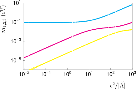
Figure 2: neutrino masses

The BRpV model produces a hierarchical mass spectrum for almost all choices of parameters. The largest mass can be estimated by the tree level value using Eq. (18). Correct $\Delta m^{2}_{\mathsc{atm}}$ can be easily obtained by an appropriate choice of $|\vec{\Lambda}|$. The mass scale for the solar neutrinos is generated at 1–loop level and therefore depends in a complicated way in the model parameters. We will see below how to get an approximate formula for the solar mass valid for most cases of interest. Here we just present in Fig. 2, for illustration purposes, the plot of the three eigenstates as a function of the parameter $\epsilon^{2}/|\Lambda|$, for a particular values of the SUSY parameters, $m_{0}=\mu=500$ GeV, $\tan\beta=5$, $B=-A=m_{0}$. For the R-parity parameters we took $|\vec{\Lambda}|=0.16$ GeV, $10*\Lambda_{e}=\Lambda_{\mu}=\Lambda_{\tau}$ and $\epsilon_{1}=\epsilon_{2}=\epsilon_{3}$.

4.2 The mixings

Now we turn to the discussion of the mixing angles. As can be seen from Fig. 2, if $\epsilon^{2}/|\vec{\Lambda}|\ll 100$, then the 1–loop corrections are not larger than the tree level results. In this case the flavor composition of the 3rd mass eigenstate is approximately given by

$$U_{\alpha 3}\approx\Lambda_{\alpha}/|\vec{\Lambda}|$$ (26)

As the atmospheric and reactor neutrino data tell us that $\nu_{\mu}\rightarrow\nu_{\tau}$ oscillations are preferred over $\nu_{\mu}\rightarrow\nu_{e}$, we conclude that

$$\Lambda_{e}\ll\Lambda_{\mu}\simeq\Lambda_{\tau}$$ (27)

are required for BRpV to fit the data. This is sown in Fig. 3 a). We cannot set all the $\Lambda_{i}$ equal, because in this case $U_{e3}$ would be too large contradicting the CHOOZ result as shown in Fig. 3 b).

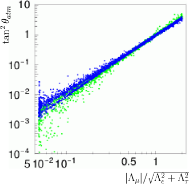
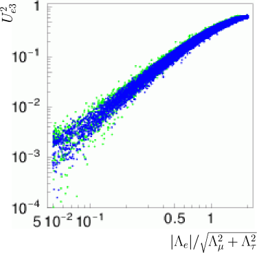
Figure 3: a) Atmospheric angle as a function of $|\Lambda_{\mu}|/\sqrt{\Lambda^{2}_{e}+\Lambda^{2}_{\tau}}$. b) $U^{2}_{e3}$ as a function of $|\Lambda_{e}|/\sqrt{\Lambda^{2}_{\mu}+\Lambda^{2}_{\tau}}$.

We have then two scenarios. In the first one, that we call the mSUGRA case, we have universal boundary conditions of the soft SUSY breaking terms. In this case we can show [11, 12] that

$$\frac{\epsilon_{e}}{\epsilon_{\mu}}\simeq\frac{\Lambda_{e}}{\Lambda_{\mu}}$$ (28)

Then from Fig. 3 b) and the CHOOZ constraint on $U^{2}_{e3}$, we obtain that both ratios in Eq. (28) have to be small. Then from Fig. 4 we conclude that the only possibility is the small angle mixing solution for the solar neutrino problem. In the second scenario, which we call the MSSM case, we consider non–universal boundary conditions of the soft SUSY breaking terms. We have shown that even a very small deviation from universality (less then 1%) of the soft parameters at the GUT scale relaxes this constraint. In this case

$$\frac{\epsilon_{e}}{\epsilon_{\mu}}\not=\frac{\Lambda_{e}}{\Lambda_{\mu}}$$ (29)

Then we can have at the same time small $U_{e3}^{2}$ determined by $\Lambda_{e}/\Lambda_{\mu}$ as in Fig. 3 b) and large $\tan^{2}(\theta_{\mathsc{sol}})$ determined by $\epsilon_{e}/\epsilon_{\mu}$ as in Fig. 4 b). After the Kamland and SNO salt results, this is the only scenario consistent with the data.

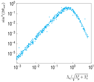
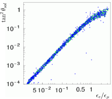
Figure 4: Solar angle as function of: a) $|\Lambda_{e}|/\sqrt{\Lambda^{2}_{\mu}+\Lambda^{2}_{\tau}}$  ; b) $\epsilon_{e}/\epsilon_{\mu}$.

5 Approximate formulas for the solar mass and mixing

In all the previous analysis we used a numerical program to evaluate the one-loop masses and mixings. It is however desirable to have analytical approximate results that can give us quickly the most important contributions. We have identified that these are the bottom-sbottom loops and the charged scalar-charged fermion loops. Then, by expanding in powers of the small R-Parity breaking parameters $\epsilon_{i}$, we get approximate formulas for the solar mass scale and mixing angle as we will explain below.

5.1 Bottom-sbottom loops

The contribution from the bottom-sbottom loop can be expressed as[14],

$$\Delta M_{ij}=-{{N_{c}m_{b}}\over{16\pi^{2}}}2s_{\tilde{b}}c_{\tilde{b}}h_{b}^{2}\Delta B_{0}^{\tilde{b}_{1}\tilde{b}_{2}}\left[\displaystyle\frac{\tilde{\epsilon}_{i}\tilde{\epsilon}_{j}}{\mu^{2}}+a_{3}b\left(\tilde{\epsilon}_{i}\delta_{j3}+\tilde{\epsilon}_{j}\delta_{i3}\right)|\vec{\Lambda}|+\left(a_{3}^{2}+\frac{a_{L}a_{R}}{h^{2}_{b}}\right)\delta_{i3}\delta_{j3}|\vec{\Lambda}|^{2}\right]\,,$$ (30)

where $\widetilde{\epsilon}_{i}$ are the $\epsilon_{i}$ in the basis where the tree level neutrino mass matrix is diagonal,

$$\widetilde{\epsilon}_{i}=\left(V_{\nu}^{(0)T}\right)^{ij}\epsilon_{j}\,,$$ (31)

the $a_{i}$ are functions of the SUSY parameters, and

$$\Delta B_{0}^{\tilde{b}_{1}\tilde{b}_{2}}=B_{0}(0,m_{b}^{2},m_{\tilde{b}_{1}}^{2})-B_{0}(0,m_{b}^{2},m_{\tilde{b}_{2}}^{2})\,.$$ (32)

The different contributions can be understood as coming from different types of insertions as shown in Fig. 5. In this figure open circles correspond to small R-parity violating projections, full circles to R-parity conserving projections, and open circles with a cross inside to mass insertions which flip chirality. With this understanding one can make a one to one correspondence between Eq. (30) and Fig. 5.

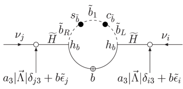
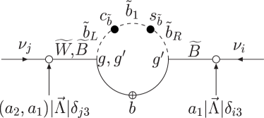
Figure 5: Bottom-sbottom loop and different types of insertions.

5.2 Charged Scalar-Charged Fermion Loops

Here the situation is much more complicated. As the charged scalars are now combinations of the six sleptons and of the two MSSM charged Higgs bosons we have many more particles that can be exchanged. For instance, the contribution from the staus is given in Fig. 6. We see that, even for the staus, we have more diagrams than for the case of the bottom-sbottom loop. This is due to the fact that the breaking of R-parity is in the leptonic sector of the theory. So we can have R-parity violating insertions both on the external neutrino legs as well as in the particles circulating in the loop. A complete description of all the terms contributing to this loop can be found in Ref.[14], where one can also find the analytical expressions.

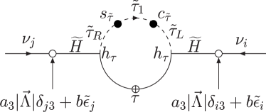
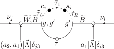
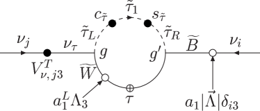
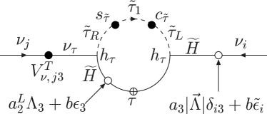
Figure 6: Charged scalar loops: the stau contribution.

5.3 Analytical vs Numerical results

We now compare the approximate analytical formulas with the full numerical calculation. This is shown in Fig. 7. On the left panel we consider a data sample where the neutralino is the Lightest Supersymmetric Particle (LSP). Shown are also the bands for LOW and LMA solutions of the solar neutrino problem, as well as the much narrower band obtained after the recent Kamland [8] and SNO salt [9] results. On the right panel we have the same situation for a data sample where the scalar tau is the LSP. We see that the agreement is specially good (better than 10%), just in the region which is compatible with the most recent data.

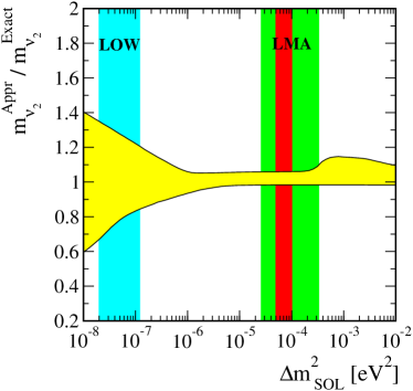
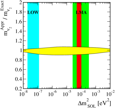
Figure 7: Comparison between the analytical and numerical results for the solar mass. In the left panel the LSP=$\chi^{0}$ while in the right panel the LSP=$\tilde{\tau}$. The red (dark) band corresponds to the latest neutrino data [10].

5.4 Simplified approximation formulas

In the basis where the tree-level neutrino mass matrix is diagonal the mass matrix at one–loop level can be written as

$$\widetilde{m}_{\nu}=V_{\nu}^{(0)T}m_{\nu}V_{\nu}^{(0)}=\left(\begin{array}[]{ccc}c_{1}\widetilde{\epsilon}_{1}\widetilde{\epsilon}_{1}&c_{1}\widetilde{\epsilon}_{1}\widetilde{\epsilon}_{2}&c_{1}\widetilde{\epsilon}_{1}\widetilde{\epsilon}_{3}\\[5.69054pt] c_{1}\widetilde{\epsilon}_{2}\widetilde{\epsilon}_{1}&c_{1}\widetilde{\epsilon}_{2}\widetilde{\epsilon}_{2}&c_{1}\widetilde{\epsilon}_{2}\widetilde{\epsilon}_{3}\\ c_{1}\widetilde{\epsilon}_{3}\widetilde{\epsilon}_{1}&c_{1}\widetilde{\epsilon}_{3}\widetilde{\epsilon}_{2}&c_{0}|\vec{\Lambda}|^{2}+c_{1}\widetilde{\epsilon}_{3}\widetilde{\epsilon}_{3}\end{array}\right)+\cdots$$

where

$$c_{0} = \frac{M_{1}g^{2}+M_{2}{g^{\prime}}^{2}}{4\,\textrm{det}({\cal M}_{\chi^{0}})}$$ (33)

$$c_{1} = \frac{3}{16\pi^{2}}\,\sin(2\theta_{\tilde{b}})\,m_{b}\,\Delta B_{0}^{\tilde{b}_{2}\tilde{b}_{1}}\ \frac{1}{\mu^{2}}$$ (34)

The dots in Eq. (5.4) correspond to the terms that are not proportional to the $\tilde{\epsilon}_{i}\times\tilde{\epsilon}_{j}$ structure, as can be seen from Eq. (30). Assuming that the bottom-sbottom loop dominates, the $\tilde{\epsilon}_{i}\times\tilde{\epsilon}_{j}$ structure is dominant, and the matrix can be diagonalized approximately under the condition

$$x\equiv\frac{c_{1}|\vec{\widetilde{\epsilon}}|^{2}}{c_{0}|\vec{\Lambda}|^{2}}\ll 1$$ (35)

Then we get

$$m_{\nu_{2}}\simeq\frac{3}{16\pi^{2}}\sin(2\theta_{\tilde{b}})m_{b}\Delta B_{0}^{\tilde{b}_{2}\tilde{b}_{1}}\ \frac{({\tilde{\epsilon}}_{1}^{2}+{\tilde{\epsilon}}_{2}^{2})}{\mu^{2}}$$ (36)

and

$$\tan^{2}\theta{sol}=\frac{\widetilde{\epsilon}_{1}^{2}}{\widetilde{\epsilon}_{2}^{2}}$$ (37)

The results for the masses are presented in Fig. 8.

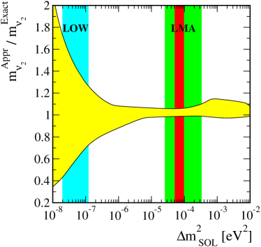
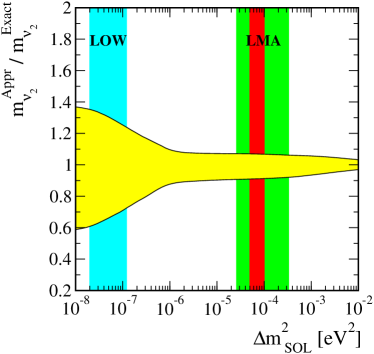
Figure 8: Comparison between the simplified analytical formulas and numerical results for the solar mass. In the left panel the LSP=$\chi^{0}$ while in the right panel the LSP=$\tilde{\tau}$. The red (dark) band corresponds to the latest neutrino data [10].

As in Fig. 7, on the left panel we have the data set where the neutralino is the LSP while on the right panel the LSP is the stau. We see that the agreement is fairly good, particularly in the region allowed by the present data.

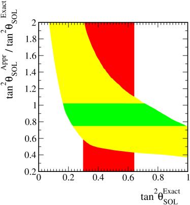
Figure 9: Comparison between the simplified analytical formulas and numerical results for the solar angle. In the left panel we present all points, and show in green the band that corresponds to more than 90% of the points. In the right panel we show all the points that have $\sin(2\theta_{\tilde{b}})\Delta B_{0}^{\tilde{\tau}_{2}\tilde{\tau}_{1}}>0.02$. The red (dark) band corresponds to the latest neutrino data [10].

For the solar angle the results are shown in Fig. 9. We see that the agreement is not as good as for the masses, even if we restrict ourselves to the present allowed values of $\tan^{2}\theta_{\hbox{\scriptsize SOL}}$, shown by the red (dark) band (it corresponds to $3\sigma$ errors as taken from [10]) on the figure. However, as we can see on the left panel, for more of 90% of the points the agreement is within 20%. This corresponds to the cases where the bottom-sbottom loop dominates as can be seen on the right panel, where we applied the cut $\sin(2\theta_{\tilde{b}})\Delta B_{0}^{\tilde{\tau}_{2}\tilde{\tau}_{1}}>0.02$ to ensure that the bottom-sbottom loop is not negligible.

So, in summary, we can say that the simplified approximate formulas of Eq. (36) and Eq. (37) give a very good approximation of the full result for most of the cases. Only in the case when the bottom-sbottom loop is not the dominant diagram (small mixing) we get large deviations.

6 Rare radiative lepton decays

As the parameters involved in the R–parity violating operator are constrained in order to predict neutrino masses in the sub-eV range, we have addressed [22] the question of whether this operator will induce rates for charged LFV processes of experimental interest. Some of them occur at tree–level such as double $\beta$ decay [23, 24] and $\mu-e$ conversion in nuclei [25]. One loop LFV decays as $l_{j}\rightarrow l_{i}\gamma$ become interesting on this framework due to the experimental interest in improving the current limits [26]:

$$BR(\mu\to e\gamma) < 1.2\times 10^{-11}$$

$$BR(\tau\to\mu\gamma) < 1.1\times 10^{-6}$$

$$BR(\tau\to e\gamma) < 2.7\times 10^{-6}.$$ (38)

We have shown that the predictions for the last two processes are much lower than the above limits and will not constrain the BRpV model. For $\mu\rightarrow e\gamma$ the predictions are compatible with the current limit but could begin to constrain the model for the bounds that will be reached in current [27] or planned experiments [28], if only the atmospheric neutrino data were taken in account. However, the requirement that the one–loop induced $\Delta m^{2}_{\mathsc{sol}}$ is in agreement with the solar neutrino data, implies that the predicted rates for $\mu\rightarrow e\gamma$ will not be visible [22], even in those new experiments. This can be seen in Fig. 10, where it is shown the contour plot for BR($\mu\rightarrow e\gamma$) as well as the maximum values of $\epsilon_{1},\epsilon_{2}$ compatible with the solar neutrino mass. So, in conclusion, the experimental constraints on these rare decays do not constrain the BRpV model.

Figure 10: Contour plots for BR($\mu\rightarrow e\gamma$). The dashed line corresponds to $m_{\nu_{2}}=0.01$ eV.

7 Probing Neutrino Mixing via SUSY Decays

After having shown, in the previous sections, that the BRpV model produces an hierarchical mass spectrum for the neutrinos that can accommodate the present data for neutrino masses and mixings, we now turn to accelerator physics and will show how the neutrino properties can be probed by looking at the decays of supersymmetric particles.

If R-parity is broken the LSP will decay. If the LSP decays then cosmological and astrophysical constraints on its nature no longer apply. Thus, within R-parity violating SUSY, a priori any superparticle could be the LSP. In the constrained version of the MSSM (mSUGRA boundary conditions) one finds only two candidates for the LSP, namely the lightest neutralino or one of the right sleptons, in particular the right scalar tau. Therefore we will consider below, in detail, these two cases together with the possibility that a light scalar top can have sizeable R-parity violating decays. However, if we depart from the mSUGRA scenario, it has been shown recently[29] that the LSP can be of other type, like a squark, gluino, chargino or even a scalar neutrino. In section 7.4 we will briefly review their results.

7.1 Probing Neutrino Mixing via Neutralino Decays

If R-parity is broken, the neutralino is unstable and it will decay through the following channels: $\tilde{\chi}^{0}_{1}\to\nu_{i}\,\nu_{j}\,\nu_{k},\ \nu_{i}\,q\,\bar{q},\ \nu_{i}\,l^{+}_{j}\,l^{-}_{k},\ l^{\pm}_{i}\,q\,\bar{q}^{\prime},\ \nu_{i}\,\gamma$. It was shown in Ref. [13], that the neutralino decays well inside the detectors and that the visible decay channels are quite large. This is shown in Fig. 11, where in the left panel we have the neutralino decay length and on the right panel its invisible branching ratio. We see that the invisible branching ratio stays always below 10%, allowing most of the channels to be seen.

Figure 11: In the left panel we show the neutralino decay length. In the right panel it is shown the invisible neutralino branching ratio.

We have shown in the previous sections that the ratios $|\Lambda_{i}/\Lambda_{j}|$ and $|\epsilon_{i}/\epsilon_{j}|$ were very important in the choice of solutions for the neutrino mixing angles. What is exciting now, is that these ratios can be measured in accelerator experiments. In the left panel of Fig. 12 we show the ratio of branching ratios for semileptonic neutralino decays into muons and taus: $BR(\chi\to\mu q^{\prime}\bar{q})/BR(\chi\to\tau q^{\prime}\bar{q}$) as function of $\tan^{2}\theta_{\mathsc{atm}}$. We can see that there is a strong correlation. The spread in this figure can in fact be explained by the fact that we do not know the SUSY parameters and are scanning over the allowed parameter space. This is illustrated in the right panel where we considered that SUSY was already discovered with the following values for the parameters,

$$M_{2}=120\,GeV,\mu=500\,GeV,\tan\beta=5,m_{0}=500\,GeV,A=-500\,GeV$$ (39)

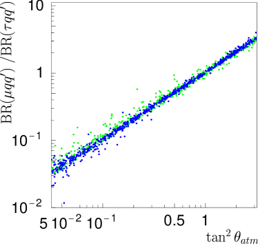
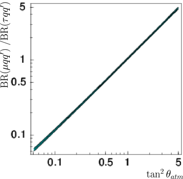
Figure 12: Ratios of semileptonic branching ratios as a function of $\tan^{2}\theta_{\mathsc{atm}}$. On the left for random SUSY values and on the right for the SUSY point of Eq. (39).

We see that the correlation is now extremely good and a measure of those semileptonic branching ratios will be an important test for the model.

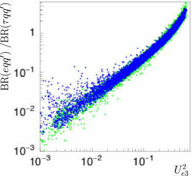
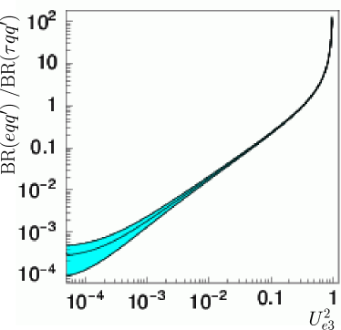
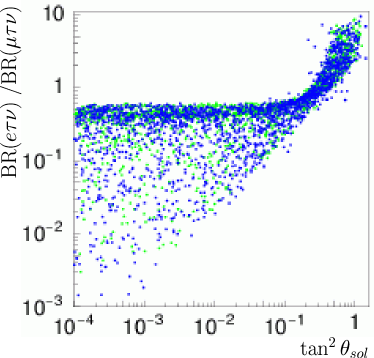
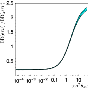
Figure 13: Correlation of neutralino decays with $U^{2}_{e3}$ (top row) and with the solar angle (bottom row). On the left column we made a random scan over the SUSY parameter space, while on the right the parameters from Eq. (39) were assumed.

By looking at other decays we can look at other neutrino parameters, as is indicated in Fig. 13. On the top row we have the correlation with $U^{2}_{e3}$ and on the bottom row the correlation with the solar angle. As before, the left panels correspond to a random scan over the SUSY parameter space, while on the right panels we have assumed that SUSY was already discovered. As an example we took the SUSY parameters in Eq. (39).

7.2 Probing Neutrino Mixing via Charged Lepton Decays

After considering the case of the LSP being the neutralino, for completeness, we have also studied [15] the case where a charged scalar lepton, most probably the scalar tau, is the LSP. We have considered the production and decays of ${\tilde{\tau}}$, ${\tilde{e}}$ and ${\tilde{\mu}}$, and have shown that also for the case of charged sleptons as LSPs they will decay well inside the detector. This is shown in Fig. 14, where on the left panel we show the production cross sections and on the right panel the decay lengths for all the sleptons.

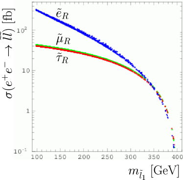
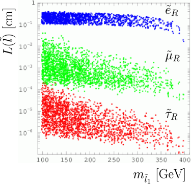
Figure 14: a)$e^{+}e^{-}\to{\tilde{l}}{\tilde{l}}$ production cross section at a Linear Collider $\sqrt{s}=0.8\hbox{TeV}$, b) Charged slepton decay length at a linear collider with $\sqrt{s}=0.8\hbox{TeV}$.

After showing that the sleptons will decay inside the detector we can correlate branching ratios with neutrino properties. This is shown in Fig. 15 where the branching ratios of the scalar taus are correlated with the solar angle, showing a strong correlation.

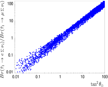
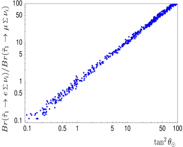
Figure 15: Ratios of branching ratios for scalar tau decays versus $\tan^{2}\theta_{\odot}$. The left panel shown all data points, the right one refers only to data points with $\epsilon_{2}/\epsilon_{3}$ restricted to the range [0.9,1.1].

7.3 Stop Decays and the Solar Angle

It was shown [16] that the stop decays are complementary to $\chi^{0}$ decays as probes of the neutrino properties. The semileptonic decays of the stop can be important as it is shown in the left panel of Fig. 16, taken from Ref. [16], where it is plotted the $\tan\beta$ dependence of the branching ratio for the decay of $\tilde{t}_{1}$ into $b\tau^{+}$ for several values of the neutrino mass. For $m_{\nu_{3}}=0.06\,$eV, the $B(\tilde{t}_{1}\to b\,\tau)$ is still above $0.1\%$ if $\tan\beta$ is not too large. In the right panel of Fig. 16 we show the ratio of B$({\tilde{t}}_{1}\to b\,e^{+})/$B$({\tilde{t}}_{1}\to b\,\mu^{+})$ versus $(\epsilon_{1}/\epsilon_{2})^{2}$ for different values of $\cos\theta_{\tilde{t}}$. For definiteness we have fixed the heaviest neutrino mass at the best-fit value indicated by the atmospheric neutrino anomaly. One can see that the dependence is nearly linear even for rather small $\cos\theta_{\tilde{t}}$. One sees from the figure that, as long as $\cos\theta_{\tilde{t}}\gtrsim 10^{-2}$ there is a good degree of correlation between the branching ratios into $B(\tilde{t}_{1}\to b\,e^{+})$ and $B(\tilde{t}_{1}\to b\,\mu^{+})$ and the ratio $(\epsilon_{1}/\epsilon_{2})^{2}$. Thus by measuring these branchings one will get information on the solar neutrino mixing, since $\tan^{2}\theta_{\mathsc{sol}}$ is proportional to $(\epsilon_{1}/\epsilon_{2})^{2}$ [11]. As a result in this model one can directly test the solution of the solar neutrino problem against the lighter stop decay pattern.

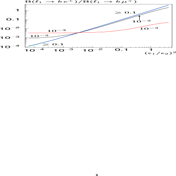
Figure 16: On the left panel we plot the branching ratios for ${\tilde{t}}_{1}$ decays for $m_{{\tilde{t}}_{1}}=220$ GeV, $\mu=500$ GeV, $M=240$ GeV, and $m_{\nu}=100$, 1 and $0.06\,$eV for $\cos\theta_{\tilde{t}}=-0.8$. On the right panel we plot the ratios: $\mbox{B}({\tilde{t}}_{1}\to be^{+})/\mbox{B}({\tilde{t}}_{1}\to b\mu^{+})$ as a function of $(\epsilon_{1}/\epsilon_{2})^{2}$ for $m_{\nu_{3}}=0.6$ eV and $|\cos\theta_{\tilde{t}}|\geq 0.1,0.01,10^{-3}$. These plots were taken from Ref. [16]

This is also complementary to the case of neutralino decays considered in section 7.1. In that case the sensitivity is mainly to atmospheric mixing, as opposed to solar mixing as can be seen from Figs. 12 and 13. Testing the solar mixing in neutralino decays at a collider experiment requires more detailed information on the complete spectrum to test the solar angle [13]. In contrast we have obtained here a rather neat connection of stop decays with the solar neutrino physics.

7.4 Other LSP decays

As we discussed in the introduction to this section, if we depart from the mSUGRA scenario, then the LSP can be of other type, like a squark, gluino, chargino or even a scalar neutrino, as it has been shown recently in Ref. [29]. As the decays of these LSP’s will always depend on the parameters that violate R-parity and induce neutrino masses and mixings, it is possible to correlate branching ratios to the neutrino properties. This is shown in Fig. 17 taken from Ref [29]. On the left panel we consider the case of chargino decays and show $BR(\tilde{\chi}^{+}\rightarrow\mu\bar{c}c)/BR(\tilde{\chi}^{+}\rightarrow\tau\bar{c}c)$ as a function of the ratio $(\Lambda_{2}/\Lambda_{3})^{2}$. As we saw in section 4, this last ratio is correlated with the atmospheric angle. So, by looking at the chargino decays one can test the atmospheric mixing angle. In fact, as the authors of Ref [29] have shown, one can use the already very precise data on the atmospheric mixing angle to put bounds on the ratios of several branching ratios of chargino decays. On the right panel we show a very strong correlation for the solar mixing angle obtained[29] with the decays of squarks. Many other correlations can be obtained making the model over constrained. So, in summary, no matter what supersymmetric particle is the LSP, measurements of branching ratios at future accelerators will provide a definite test of the BRpV model as a viable model for explaining the neutrino properties.

Figure 17: Left panel: ratios of branching ratios for chargino decays versus $(\Lambda_{2}/\Lambda_{3})^{2}$; Right panel: ratios of branching ratios for squark decays versus $\tan^{2}\theta\mathsc{sol}$. These plots were taken from Ref. [29].

8 Conclusions

The Bilinear R-Parity Violation Model is a simple extension of the MSSM that leads to a very rich phenomenology. Hopefully, it will be an effective model for the more theoretically attractive case where R-parity is spontaneously broken [31, 32].

We have calculated the one–loop corrected masses and mixings for the neutrinos in a completely consistent way, including the RG equations and correctly minimizing the potential. We have shown that it is possible to get easily maximal mixing for the atmospheric neutrinos and large angle MSW, as it is preferred by the present neutrino data. We have also obtained approximate formulas for the solar mass and solar mixing angle, that we found to be very good, precisely in the region of parameters favored by this data.

We emphasize that the LSP decays inside the detectors, thus leading to a very different phenomenology than the MSSM. In the mSUGRA scenarios, the LSP can be either the lightest neutralino, like in the MSSM, or a charged particle, must probably the lightest stau. In both cases we have shown that ratios of the branching ratios of the LSP can be correlated with the neutrino parameters. We have also shown, that the decays of the stop can be complementary to those of the LSP for the case of the solar mixing angle.

In more general scenarios than the constrained mSUGRA, the LSP can essentially be any supersymmetric particle. However, also in these scenarios the neutrino properties can be correlated with ratios of branching ratios for these particles.

So, in summary, no matter what supersymmetric particle is the LSP measurements of branching ratios at future accelerators will provide a definite test of the BRpV model as a viable model for explaining the neutrino properties.

- [1] Super-Kamiokande, Y. Fukuda et al., Phys. Rev. Lett. 81, 1562 (1998), [hep-ex/9807003].
- [2] M. Maltoni, T. Schwetz, M. A. Tortola and J. W. F. Valle, Phys. Rev. D67, 013011 (2003), [hep-ph/0207227 v3 KamLAND-updated version].
- [3] M. Gonzalez-Garcia, M. Maltoni, C. Pena-Garay and J. W. F. Valle, Phys. Rev. D63, 033005 (2001), [hep-ph/0009350].
- [4] CHOOZ, M. Apollonio et al., Phys. Lett. B466, 415 (1999), [hep-ex/9907037].
- [5] F. Boehm et al., Phys. Rev. D64, 112001 (2001), [hep-ex/0107009].
- [6] Super-Kamiokande, S. Fukuda et al., Phys. Lett. B539, 179 (2002), [hep-ex/0205075].
- [7] J. N. Bahcall, S. Basu and M. H. Pinsonneault, Phys. Lett. B433, 1 (1998), [astro-ph/9805135].
- [8] KamLAND, K. Eguchi et al., Phys. Rev. Lett. 90, 021802 (2003), [hep-ex/0212021].
- [9] SNO, S. N. Ahmed et al., nucl-ex/0309004.
- [10] M. Maltoni, T. Schwetz, M. A. Tortola and J. W. F. Valle, hep-ph/0309130.
- [11] J. C. Romao, M. A. Diaz, M. Hirsch, W. Porod and J. W. F. Valle, Phys. Rev. D61, 071703 (2000), [hep-ph/9907499].
- [12] M. Hirsch, M. A. Diaz, W. Porod, J. C. Romao and J. W. F. Valle, Phys. Rev. D62, 113008 (2000), [hep-ph/0004115], Err-ibid.D65:119901,2002.
- [13] W. Porod, M. Hirsch, J. Romao and J. W. F. Valle, Phys. Rev. D63, 115004 (2001), [hep-ph/0011248].
- [14] M. A. Diaz, M. Hirsch, W. Porod, J. C. Romao and J. W. F. Valle, Phys. Rev. D68, 013009 (2003), [hep-ph/0302021].
- [15] M. Hirsch, W. Porod, J. C. Romao and J. W. F. Valle, Phys. Rev. D66, 095006 (2002), [hep-ph/0207334].
- [16] D. Restrepo, W. Porod and J. W. F. Valle, Phys. Rev. D64, 055011 (2001), [hep-ph/0104040].
- [17] M. A. Diaz, J. C. Romao and J. W. F. Valle, Nucl. Phys. B524, 23 (1998), [hep-ph/9706315].
- [18] F. de Campos, M. A. Garcia-Jareno, A. S. Joshipura, J. Rosiek and J. W. F. Valle, Nucl. Phys. B451, 3 (1995), [hep-ph/9502237].
- [19] A. G. Akeroyd, M. A. Diaz, J. Ferrandis, M. A. Garcia-Jareno and J. W. F. Valle, Nucl. Phys. B529, 3 (1998), [hep-ph/9707395].
- [20] T. Banks, Y. Grossman, E. Nardi and Y. Nir, Phys. Rev. D52, 5319 (1995), [hep-ph/9505248].
- [21] G. Passarino and M. J. G. Veltman, Nucl. Phys. B160, 151 (1979).
- [22] D. F. Carvalho, M. E. Gomez and J. C. Romao, Phys. Rev. D65, 093013 (2002), [hep-ph/0202054].
- [23] A. Faessler, S. Kovalenko and F. Simkovic, Phys. Rev. D58, 055004 (1998), [hep-ph/9712535].
- [24] M. Hirsch and J. W. F. Valle, Nucl. Phys. B557, 60 (1999), [hep-ph/9812463].
- [25] A. Faessler, T. S. Kosmas, S. Kovalenko and J. D. Vergados, Nucl. Phys. B587, 25 (2000).
- [26] Particle Data Group, D. E. Groom et al., Eur. Phys. J. C15, 1 (2000).
- [27] J. Yashima et al., Prepared for Joint U.S. / Japan Workshop on New Initiatives in Muon Lepton Flavor Violation and Neutrino Oscillation with High Intense Muon and Neutrino Sources, Honolulu, Hawaii, 2-6 Oct 2000.
- [28] Y. Kuno, Lepton flavor violation experiments at kek/jaeri joint project of high intensity proton machine, 2000, Proceedings of Workshop of LOWNU/NOON 2000, Tokyo, December 4-8, 2000.
- [29] M. Hirsch and W. Porod, hep-ph/0307364.
- [30] B. Mukhopadhyaya, S. Roy and F. Vissani, Phys. Lett. B443, 191 (1998), [hep-ph/9808265].
- [31] J. C. Romao, C. A. Santos and J. W. F. Valle, Phys. Lett. B288, 311 (1992).
- [32] J. C. Romao and J. W. F. Valle, Nucl. Phys. B381, 87 (1992).