Abstract

We demonstrate how the interplay of a future $e^{+}e^{-}$ LC at its first stage with $\sqrt{s}\;\raisebox{-3.87495pt}{$\textstyle\stackrel{{\scriptstyle\textstyle<}}{{\sim}}$}\;500$ GeV and of the LHC could lead to a precise determination of the fundamental SUSY parameters in the gaugino/higgsino sector without assuming a specific supersymmetry breaking scheme. We demonstrate this for the benchmark scenario SPS1a, taking into account realistic errors for the masses and cross sections measured at the LC with polarised beams, including errors coming from polarisation measurements, and mass measurements at the LHC. The results clearly demonstrate the complementarity of the LHC and LC, and the benefit from the joint analyses of their data.

1 Introduction

Supersymmetry (SUSY) is one of the best motivated extensions of the Standard Model (SM). However, since SUSY has to be broken even the minimal version, the unconstrained MSSM, has 105 new parameters. SUSY analyses at future experiments, at the LHC and at a future Linear Collider (LC), will have to focus on the determination of these parameters in as model-independent a way as possible [1].

With so many new parameters clear strategies will be needed in analysing the experimental data [2]. An interesting possibility to resolve the new physics is to start with the gaugino/higgsino particles which are expected to be among the lightest SUSY particles. At tree level, this sector depends only on 4 parameters: $M_{1}$, $M_{2}$, $\mu$ and $\tan\beta$ – the U(1) and SU(2) gaugino masses, the higgsino mass parameter and the ratio of the vacuum expectations of the two Higgs fields, respectively.

Some strategies have been worked out for the determination at the tree level the parameters $M_{2}$, $M_{1}$, $\mu$, $\tan\beta$ even if only the light gaugino/higgsino particles, $\tilde{\chi}^{0}_{1}$, $\tilde{\chi}^{0}_{2}$ and $\tilde{\chi}^{\pm}_{1}$ were kinematically accessible at the first stage of the LC [3]. In this report we demonstrate how such an LC analysis could be strengthened if in addition some information on the mass of the heaviest neutralino the LHC is available. We consider three scenarios: (i) stand alone LC data, (ii) when the LC data are supplemented by the heavy neutralino mass estimated from the LHC data, and (iii) joint analysis of the LC and LHC data. The results in the last scenario will clearly demonstrate the essentiality of the LHC and LC and the benefit from the joint analysis of their data.

In order to work out this hand-in-hand LHC+LC analysis for determining the tree-level SUSY parameters, we assume that only the first phase of a LC with a tunable energy up to $\sqrt{s}=500$ GeV would overlap with the LHC running. Furthermore, we assume an integrated luminosity of $\int{\cal L}\sim 500$ fb^-1 and polarised beams with $P(e^{-})=\pm 80\%$, $P(e^{+})=\pm 60\%$. In the following $\sigma_{L}$ will refer to cross sections obtained with $P(e^{-})=-80\%$, $P(e^{+})=+60\%$, and $\sigma_{R}$ with $P(e^{-})=+80\%$, $P(e^{+})=-60\%$. We restrict ourselves to the CP conserving chargino/neutralino sector and take the SPS1a as a working benchmark [4]; the inclusion of CP violating phases will be considered elsewhere.

Before presenting our results on the parameter determination, we first briefly recapitulate the main features of chargino and neutralino sectors and sketch our strategy.

2 The gaugino/higgsino sector

2.1 Chargino sector

The mass matrix of the charged gaugino $\tilde{W}^{\pm}$ and higgsino $\tilde{H}^{\pm}$ is given by

$${\cal M}_{C}=\left(\begin{array}[]{cc}M_{2}&\sqrt{2}m_{W}\cos\beta\\[5.69054pt] \sqrt{2}m_{W}\sin\beta&\mu\end{array}\right)$$ (3)

As a consequence of possible field redefinitions, the parameter $M_{2}$ can be chosen real and positive. The two charginos $\tilde{\chi}^{\pm}_{1,2}$ are mixtures of the charged SU(2) gauginos and higgsinos. Since the mass matrix ${\cal M}_{C}$ is not symmetric, two different unitary matrices acting on the left– and right–chiral $(\tilde{W},\tilde{H})_{L,R}$ two–component states

$$\left(\begin{array}[]{c}\tilde{\chi}^{-}_{1}\\ \tilde{\chi}^{-}_{2}\end{array}\right)_{L,R}=U_{L,R}\left(\begin{array}[]{c}\tilde{W}^{-}\\ \tilde{H}^{-}\end{array}\right)_{L,R}$$ (8)

define charginos as mass eigenstates. For real ${\cal M}_{C}$ the unitary matrices $U_{L}$ and $U_{R}$ can be parameterised as

$$U_{L,R}=\left(\begin{array}[]{cc}\cos\Phi_{L,R}&\sin\Phi_{L,R}\\ -\sin\Phi_{L,R}&\cos\Phi_{L,R}\end{array}\right)$$ (11)

The mass eigenvalues $m^{2}_{\tilde{\chi}^{\pm}_{1,2}}$ and the mixing angles are given by

$$m^{2}_{\tilde{\chi}^{\pm}_{1,2}} = \frac{1}{2}(M^{2}_{2}+\mu^{2}+2m^{2}_{W}\mp\Delta_{C})$$

$$\cos 2\phi_{L,R} = -(M_{2}^{2}-\mu^{2}\mp 2m^{2}_{W}\cos 2\beta)/\Delta_{C}$$

where $\Delta_{C}=[(M^{2}_{2}-\mu^{2})^{2}+4m^{4}_{W}\cos^{2}2\beta+4m^{2}_{W}(M^{2}_{2}+\mu^{2})+8m^{2}_{W}M_{2}\mu\sin 2\beta]^{1/2}$.

The $e^{+}e^{-}\to\tilde{\chi}^{\pm}_{i}\tilde{\chi}^{\mp}_{j}$ production processes occur via the s-channel $\gamma$, $Z^{0}$ and the t-channel $\tilde{\nu}_{e}$ exchange. Since the two mixing angles $\Phi_{L,R}$ enter the couplings in the $\tilde{\chi}\tilde{\chi}Z$ and $e\tilde{\chi}\tilde{\nu}_{e}$ vertices, the chargino production cross sections $\sigma^{\pm}\{ij\}=\sigma(e^{+}e^{-}\to\tilde{\chi}^{\pm}_{i}\tilde{\chi}^{\mp}_{j})$ are bilinear functions of $\cos 2\Phi_{L,R}$ [6] and can be written as

$$\sigma^{\pm}\{ij\}=c_{1}\cos^{2}2\Phi_{L}+c_{2}\cos 2\Phi_{L}+c_{3}\cos^{2}2\Phi_{R}+c_{4}\cos 2\Phi_{R}+c_{5}\cos 2\Phi_{L}\cos 2\Phi_{R}+c_{6}$$ (12)

We derived the coefficients $c_{1},\ldots,c_{6}$ for the lightest chargino pair production cross section, see eq. (12) in the Appendix.

2.2 Neutralino sector

The neutralino mixing matrix in the $\{\tilde{\gamma},\tilde{Z}^{0},\tilde{H}^{0}_{1},\tilde{H}^{0}_{2}\}$ basis is given by

$${\cal M}_{N}=\left(\begin{array}[]{cccc}M_{1}\cos^{2}_{W}+M_{2}\sin^{2}_{W}&(M_{2}-M_{1})\sin_{W}\cos_{W}&0&0\\[5.69054pt] (M_{2}-M_{1})\sin_{W}\cos_{W}&M_{1}\sin^{2}_{W}+M_{2}\cos^{2}_{W}&m_{Z}&0\\[5.69054pt] 0&m_{Z}&\mu\sin{2\beta}&-\mu\cos{2\beta}\\[5.69054pt] 0&0&-\mu\cos{2\beta}&-\mu\sin{2\beta}\end{array}\right)\$$ (17)

The neutralino eigenvectors and their masses are obtained with the 4$\times$4 diagonalisation matrix $N$:

$$N{\cal M}_{N}N^{\dagger}={\sf diag}\{m_{\tilde{\chi}^{0}_{1}},\ldots,m_{\tilde{\chi}^{0}_{4}}\}$$ (18)

The parameter $M_{1}$ can only be determined from the neutralino sector. The characteristic equation of the mass matrix squared, ${\cal M}_{N}{\cal M}^{\dagger}_{N}$, can be written as a quadratic equation for the parameter $M_{1}$:

$$x_{i}M_{1}^{2}+y_{i}M_{1}-z_{i}=0,\quad\mbox{for}\quad i=1,2,3,4$$ (19)

where $x_{i}$, $y_{i}$, $z_{i}$ are given by:

$$x_{i} = -m_{\tilde{\chi}^{0}_{i}}^{6}+a_{41}m_{\tilde{\chi}^{0}_{i}}^{4}-a_{21}m_{\tilde{\chi}^{0}_{i}}^{2}+a_{01},$$ (20)

$$y_{i} = a_{42}m_{\tilde{\chi}^{0}_{i}}^{4}-a_{22}m_{\tilde{\chi}^{0}_{i}}^{2}+a_{02},$$ (21)

$$z_{i} = m_{\tilde{\chi}^{0}_{i}}^{8}-a_{63}m_{\tilde{\chi}^{0}_{i}}^{6}+a_{43}m_{\tilde{\chi}^{0}_{i}}^{4}-a_{23}m_{\tilde{\chi}^{0}_{i}}^{2}+a_{03},$$ (22)

The coefficients $a_{kl}$, ($k=0,2,4,6$, $l=1,2,3$), being invariants of the matrix ${\cal M}_{N}{\cal M}_{N}^{T}$, can be expressed as functions of $M_{2}$, $\mu$ and $\tan\beta$. Their explicit form is given in the Appendix.

The $e^{+}e^{-}\to\tilde{\chi}^{0}_{i}\tilde{\chi}^{0}_{j}$ production processes occur via the s-channel $Z^{0}$ and the t- and u-channel $\tilde{e}_{L}$ and $\tilde{e}_{R}$ exchanges. Since the neutralino mixing matrix $N$ is parameterised in general by 6 angles, the analytic expressions for the production cross sections are more involved. Their explicit form can be found in [3].

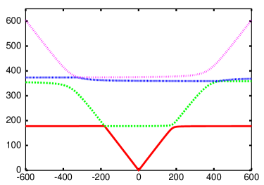
As one can see from eq. (19) for each neutralino mass $m_{\tilde{\chi}^{0}_{i}}$ one gets two solutions for $M_{1}$. In principle, a measurement of two neutralino masses and/or the cross section resolves this ambiguity. However, one has to remember that the mass eigenvalues show different sensitivity to the parameter $M_{1}$, depending on their gaugino/higgsino composition. In our scenario, the mass of the lightest neutralino $m_{\tilde{\chi}^{0}_{1}}$ depends strongly on $M_{1}$ if $M_{1}$ is in the range $-183$ GeV$<M_{1}<180$ GeV, while the others are roughly insensitive, see Fig. 1. For larger and larger $|M_{1}|$, the heavier neutralinos become more sensitive to $M_{1}$ [7].

Figure 1: $M_{1}$ dependence of the neutralino mass eigenvalues $m_{\tilde{\chi}^{0}_{i}}$, $i=1,\ldots,4$ with $M_{2}$, $\mu$ and $\tan\beta$ as in the reference scenario SPS1a.

2.3 The strategy

At the initial phase of future $e^{+}e^{-}$ linear–collider operations with polarised beams, the collision energy may only be sufficient to reach the production thresholds of the light chargino $\tilde{\chi}^{\pm}_{1}$ and the two lightest neutralinos $\tilde{\chi}^{0}_{1},\,\tilde{\chi}^{0}_{2}$. From the analysis of this restricted system, nevertheless the entire tree level structure of the gaugino/higgsino sector can be unraveled in analytical form in CP–invariant theories as follows [6, 3].

It is clear from eq.(12) that by analysing the $\tilde{\chi}^{+}_{1}\tilde{\chi}^{-}_{1}$ production cross sections with polarised beams, $\sigma^{\pm}_{L}\{11\}$ and $\sigma^{\pm}_{R}\{11\}$, the chargino mixing angles $\cos 2\Phi_{L}$ and $\cos 2\Phi_{R}$ can be determined [6]. Any two contours, $\sigma^{\pm}_{L}\{11\}$ and $\sigma^{\pm}_{R}\{11\}$ for example, will cross at least at one point in the plane between $-1\leq{\cos 2\Phi_{L}},\cos 2\Phi_{R}\leq+1$, if the chargino and sneutrino masses are known and the SUSY Yukawa coupling is identified with the gauge coupling. However, the contours, being of second order, may cross up to four times. The ambiguity can be resolved by measuring the transverse cross section $\sigma^{\pm}_{T}\{11\}$, or measuring $\sigma^{\pm}_{L}\{11\}$ and $\sigma^{\pm}_{R}\{11\}$ at different beam energies.

In the CP conserving case studied in this paper the SUSY parameters $M_{2}$, $\mu$ and $\tan\beta$ can be determined from the chargino mass $m_{\tilde{\chi}^{\pm}_{1}}$ and mixing angles ${\cos 2\Phi_{L}}$, $\cos 2\Phi_{R}$ [6]. It is convenient to define

$$p = \pm\left|\frac{\sin 2\Phi_{L}+\sin 2\Phi_{R}}{\cos 2\Phi_{L}-\cos 2\Phi_{R}}\right|$$ (23)

$$q = \frac{1}{p}\frac{\cos 2\Phi_{L}+\cos 2\Phi_{R}}{\cos 2\Phi_{L}-\cos 2\Phi_{R}}$$ (24)

Since the ${\cos 2\Phi_{L}}$ and $\cos 2\Phi_{R}$ are derived from $\tilde{\chi}^{+}_{1}\tilde{\chi}^{-}_{1}$ cross sections, the relative sign of $\sin 2\Phi_{L}$, $\sin 2\Phi_{R}$ is not determined and both possibilities in eqn.(23), (24) have to be considered. From $p,q$, the SUSY parameters are determined as follows ($r^{2}=m^{2}_{\tilde{\chi}^{\pm}_{1}}/m^{2}_{W}$):

$$M_{2} = \frac{m_{W}}{\sqrt{2}}\left[(p+q)\sin\beta-(p-q)\cos\beta\right]$$ (25)

$$\mu = \frac{m_{W}}{\sqrt{2}}\left[(p-q)\sin\beta-(p+q)\cos\beta\right]$$ (26)

$$\tan\beta = \left[\frac{p^{2}-q^{2}\pm\sqrt{r^{2}(p^{2}+q^{2}+2-r^{2})}}{(\sqrt{1+p^{2}}-\sqrt{1+q^{2}})^{2}-2r^{2}}\right]^{\eta}$$ (27)

where $\eta=1$ for $\cos 2\Phi_{R}>{\cos 2\Phi_{L}}$, and $\eta=-1$ otherwise. The parameters $M_{2}$, $\mu$ are uniquely fixed if $\tan\beta$ is chosen properly. Since $\tan\beta$ is invariant under simultaneous change of the signs of $p,q$, the definition $M_{2}>0$ can be exploited to remove this overall sign ambiguity.

The remaining parameter $M_{1}$ can be obtained from the neutralino data [3]. The characteristic equation for the neutralino mass eigenvalues eq. (19) is quadratic in $M_{1}$ if $M_{2}$, $\mu$ and $\tan\beta$ are already predetermined in the chargino sector. In principle, two neutralino masses are then sufficient to derive $M_{1}$. The cross sections $\sigma_{L,R}^{0}\{12\}$ and $\sigma_{L,R}^{0}\{22\}$ for production of ${\tilde{\chi}}^{0}_{1}{\tilde{\chi}}^{0}_{2}$ and ${\tilde{\chi}}^{0}_{2}{\tilde{\chi}}^{0}_{2}$ neutralino pairs with polarised beams can serve as a consistency check of the derived parameters.

In practice the above procedure may be much more involved due to finite experimental errors of mass and cross section measurements, uncertainties from sneutrino and selectron masses which enter the cross section expressions, errors on beam polarisation measurement, etc. In addition, depending on the benchmark scenario, some physical quantities in the light chargino/neutralino system may turn to be essentially insensitive to some parameters. For example, as seen in fig. 1, the first two neutralino masses are insensitive to $M_{1}$ if $M_{1}\gg M_{2},\,\mu$. Additional information from the LHC on heavy states, if available, can therefore be of great value in constraining the SUSY parameters.

Our strategy can be applied only at the tree level. Radiative corrections, which in the electroweak sector can be ${\cal O}$(10%), inevitably bring all SUSY parameters together [9]. Nevertheless, tree level analyses should provide in a relatively model-independent way good estimates of SUSY parameters, which can be further refined by including iteratively radiative corrections in an overall fit to experimental data.

3 SUSY parameters from the LC data

3.1 Experimental input at the LC

In this paper we adopt the SPS1a scenario defined at the electroweak scale [4]. The relevant SUSY parameters are

$$M_{1}=99.13~{}{\mbox{G}eV},\quad M_{2}=192.7~{}{\mbox{G}eV},\quad\mu=352.4~{}{\mbox{G}eV},\quad\tan\beta=10$$ (28)

The resulting chargino and neutralino masses, together with the slepton masses of the first generation, are given in table 1.

	${\tilde{\chi}^{\pm}_{1}}$	${\tilde{\chi}^{\pm}_{2}}$	${\tilde{\chi}^{0}_{1}}$	${\tilde{\chi}^{0}_{2}}$	${\tilde{\chi}^{0}_{3}}$	${\tilde{\chi}^{0}_{4}}$	${\tilde{e}_{R}}$	${\tilde{e}_{L}}$	${\tilde{\nu}_{e}}$
mass	176.03	378.50	96.17	176.59	358.81	377.87	143.0	202.1	186.0
error	0.55		0.05	1.2			0.05	0.2	0.7

Table 1: Chargino, neutralino and slepton masses in SPS1a, and the simulated experimental errors at the LC [11, 12]. It is assumed that the heavy chargino and neutralinos are not observed at the first phase of the LC operating at $\sqrt{s}\leq 500$ GeV. [All quantities are in GeV.]

Because $\tilde{\chi}^{+}_{1}$ and $\tilde{\chi}^{0}_{2}$ decay dominantly into $\tilde{\tau}$ producing the signal similar to that of stau pair production, the $\tilde{\tau}$ mass and mixing angle are also important for the study of chargino and neutralino sectors. The mass and mixing angle can be determined as $m_{\tilde{\tau}_{1}}=133.2\pm 0.30$ GeV and $\cos 2\theta_{\tau}=-0.84\pm 0.04$, and the production cross section ranges from 43 fb to 138 fb depending on the beam polarisation, see [10, 11] for details of the stau parameter measurements. We assume that the contamination of stau production events can be subtracted from the chargino and neutralino production. Below we included the statistical error to our analysis but we did not include the systematic errors.

3.2 Chargino Sector

As observables we use the light chargino mass and polarised cross sections $\sigma^{\pm}_{L}\{11\}$ and $\sigma^{\pm}_{R}\{11\}$ at $\sqrt{s}=500$ GeV and $\sqrt{s}=400$ GeV. The light charginos $\tilde{\chi}^{\pm}_{1}$ decay almost exclusively to $\tilde{\tau}^{\pm}_{1}\nu_{\tau}$ followed by $\tilde{\tau}^{\pm}_{1}\to\tau^{\pm}\tilde{\chi}^{0}_{1}$. The signature for the $\tilde{\chi}^{\pm}_{1}\tilde{\chi}^{\mp}_{1}$ production would be two tau jets in opposite hemispheres plus missing energy.

The experimental errors that we assume and take into account are:

• The measurement of the chargino mass has been simulated and the expected error is 0.55 GeV, table 1.

• With $\int{\cal L}=500$ fb^-1 at the LC, we assume 100 fb^-1 per each polarisation configuration and we take into account 1$\sigma$ statistical error.

• Since the chargino production is sensitive to $m_{\tilde{\nu}_{e}}$, we include its experimental error of 0.7 GeV.

• The measurement of the beam polarisation with an uncertainty of $\Delta P(e^{\pm})/P(e^{\pm})=0.5\%$ is assumed. This error is conservative; discussions to reach errors smaller than $0.25\%$ are underway [13].

The errors on production cross sections induced by the above uncertainties, as well as the total errors (obtained by adding individual errors in quadrature), are listed in table 2. We assume 100% efficiency for the chargino cross sections due to a lack of realistic simulations.

++++$\sqrt{s}$	400 GeV		500 GeV
($P(e^{-})$, $P(e^{+})$)	$(-80\%,+60\%)$	$(+80\%,-60\%)$	$(-80\%,+60\%)$	$(+80\%,-60\%)$
$\sigma(e^{+}e^{-}\to\tilde{\chi}^{+}_{1}\tilde{\chi}^{-}_{1})$	215.84	6.38	504.87	15.07
$\delta\sigma_{\mbox{stat}}$	1.47	0.25	2.25	0.39
$\delta\sigma_{P(e^{-})}$	0.48	0.12	1.12	0.28
$\delta\sigma_{P(e^{+})}$	0.40	0.04	0.95	0.10
$\delta\sigma_{m_{\tilde{\chi}^{\pm}_{1}}}$	7.09	0.20	4.27	0.12
$\delta\sigma_{m_{\tilde{\nu}_{e}}}$	0.22	0.01	1.57	0.04
$\delta\sigma_{\mbox{total}}$	7.27	0.35	5.28	0.51

Table 2: Cross sections $\sigma_{L,R}^{\pm}\{11\}=\sigma_{L,R}(e^{+}e^{-}\to\tilde{\chi}^{+}_{1}\tilde{\chi}^{-}_{1})$ with polarised beams $P(e^{-})=\mp 80\%$, $P(e^{+})=\pm 60\%$ at $\sqrt{s}=400$ and 500 GeV and assumed errors (in fb) corresponding to 100 fb^-1 for each polarisation configuration.

Now we can exploit the eq. (12) and draw $\cos 2\Phi_{R}=f(\cos 2\Phi_{L},\sigma^{\pm}_{L,R}\{11\})$ consistent with the predicted cross sections within the mentioned error bars, as shown in fig. 2. With the $\sqrt{s}=500$ GeV data alone two possible regions in the plane are selected. With the help of the $\sigma^{\pm}_{L}\{11\}$ at $\sqrt{s}=400$ GeV ($\sigma^{\pm}_{R}\{11\}$ is small and does not provide further constraints) the ambiguity is removed and the mixing angles are limited within the range

$$\cos 2\Phi_{L} = [0.62,0.72]$$ (29)

$$\cos 2\Phi_{R} = [0.87,0.91]$$ (30)

Figure 2: $\cos 2\Phi_{R}$ as a function of $\cos 2\Phi_{L}$ for $\sigma^{\pm}_{L}\{11\}$ at $\sqrt{s}=500$ GeV (red), and 400 GeV (green) and $\sigma^{\pm}_{R}\{11\}$ at $\sqrt{s}=500$ GeV (blue) within the error bounds (theo+exp) as given in table 2.

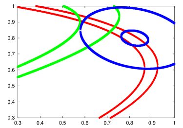
Although ${\cos 2\Phi_{L}},\cos 2\Phi_{R}$ are determined rather precisely at a few per-cent accuracy, an attempt to exploit eqns. (25)-(27) shows that $M_{2}$ is reconstructed within 10 GeV, $\mu$ within 40 GeV, and essentially no limit on $\tan\beta$ is obtained (we get $\tan\beta>6$). The main reason for this result is a relatively large error of the light chargino mass measurement due to the $\tilde{\chi}^{+}_{1}\to\tilde{\chi}^{0}_{1}\tau^{+}\nu_{\tau}$ decay mode. Several methods exploiting other sectors of the MSSM have been proposed to measure $\tan\beta$ in the high $\tan\beta$ regime [14, 10]. In the following we will exploit the neutralino sector (with eqns. (29), (30) as the allowed ranges for the chargino mixing angles) to improve constraints on $M_{2}$, $\mu$ and $\tan\beta$, and to determine $M_{1}$.

3.3 Neutralino Sector

As observables we use the two light neutralino masses and polarised cross sections $\sigma^{0}_{L,R}\{12\}$ and $\sigma^{0}_{L,R}\{22\}$ at $\sqrt{s}=400$ GeV and $\sqrt{s}=500$ GeV. Although the production of $\tilde{\chi}^{0}_{1}\tilde{\chi}^{0}_{3}$ and $\tilde{\chi}^{0}_{1}\tilde{\chi}^{0}_{4}$ pairs is kinematically accessible at $\sqrt{s}=500$ GeV, the rates are small and the heavy states ${\tilde{\chi}}^{0}_{3}$ and ${\tilde{\chi}}^{0}_{4}$ decay via cascades to many particles. Therefore we constrain our analysis to the production of the light neutralino pairs.

++++ $\sqrt{s}$	400  GeV		500 GeV
($P(e^{-})$, $P(e^{+})$)	$(-80\%,+60\%)$	$(+80\%,-60\%)$	$(-80\%,+60\%)$	$(+80\%,-60\%)$
$\sigma(e^{+}e^{-}\to\tilde{\chi}^{0}_{1}\tilde{\chi}^{0}_{2})$	148.38	20.06	168.42	20.81
$\delta\sigma_{\mbox{stat}}$	2.92	1.55	3.47	1.55
$\delta\sigma_{\mbox{bg}}$	0.44	0.02	0.31	0.03
$\delta\sigma_{P(e^{-})}$	0.32	0.05	0.37	0.06
$\delta\sigma_{P(e^{+})}$	0.28	0.001	0.31	0.01
$\delta\sigma_{m_{\tilde{\chi}^{\pm}_{1}}}$	0.21	0.30	0.16	0.26
$\delta\sigma_{m_{\tilde{e}_{L}}}$	0.20	0.01	0.17	0.01
$\delta\sigma_{m_{\tilde{e}_{R}}}$	0.00	0.01	0.00	0.01
$\delta\sigma_{\mbox{total}}$	3.0	1.58	3.52	1.57

Table 3: Cross sections $\sigma^{0}_{L,R}\{12\}=\sigma_{L,R}(e^{+}e^{-}\to\tilde{\chi}^{0}_{1}\tilde{\chi}^{0}_{2})$ with polarised beams $P(e^{-})=\mp 80\%$, $P(e^{+})=\pm 60\%$ at $\sqrt{s}=400$ and 500 GeV, and assumed errors (in fb) corresponding to 100 fb^-1 for each polarisation configuration.

	400 GeV		500 GeV
($P(e^{-})$, $P(e^{+})$)	$(-80\%,+60\%)$	$(+80\%,-60\%)$	$(-80\%,+60\%)$	$(+80\%,-60\%)$
$\sigma(e^{+}e^{-}\to\tilde{\chi}^{0}_{2}\tilde{\chi}^{0}_{2})$	85.84	2.42	217.24	6.10
$\delta\sigma_{\mbox{stat}}$	2.4	0.4	3.8	0.6
$\delta\sigma_{P(e^{-})}$	0.19	0.05	0.48	0.12
$\delta\sigma_{P(e^{+})}$	0.16	0.02	0.41	0.05
$\delta\sigma_{m_{\tilde{\chi}^{\pm}_{1}}}$	2.67	0.08	1.90	0.05
$\delta\sigma_{m_{\tilde{e}_{L}}}$	0.15	0.004	0.28	0.01
$\delta\sigma_{m_{\tilde{e}_{R}}}$	0.00	0.00	0.00	0.00
$\delta\sigma_{\mbox{total}}$	3.6	0.41	4.3	0.62

Table 4: Cross sections $\sigma^{0}_{L,R}\{22\}=\sigma_{L,R}(e^{+}e^{-}\to\tilde{\chi}^{0}_{2}\tilde{\chi}^{0}_{2})$ with polarised beams $P(e^{-})=\mp 80\%$, $P(e^{+})=\pm 60\%$ at $\sqrt{s}=400$ and 500 GeV, and assumed errors (in fb) corresponding to 100 fb^-1 for each polarisation configuration.

The neutralino $\tilde{\chi}^{0}_{2}$ decays into $\tilde{\tau}^{\pm}_{1}\tau^{\mp}$ with almost 90%, followed by the $\tilde{\tau}^{\pm}_{1}\to\tau^{\pm}\tilde{\chi}^{0}_{1}$. Therefore the final states for the $\tilde{\chi}^{\pm}_{1}\tilde{\chi}^{\mp}_{1}$ and $\tilde{\chi}^{0}_{1}\tilde{\chi}^{0}_{2}$ are the same (2$\tau$ + missing energy), however with different topology. While for the charginos, the $\tau$’s tend be in opposite hemispheres with rather large invariant mass, in the $\tilde{\chi}^{0}_{1}\tilde{\chi}^{0}_{2}$ process both $\tau$’s, coming from the $\tilde{\chi}^{0}_{2}$ decay, would be more often in the same hemisphere with smaller invariant mass. This feature allows separate the processes to some extent exploiting e.g. a cut on the opening angle between the two jets of the $\tau^{\prime}s$. However, in the case of $\tilde{\chi}^{0}_{1}\tilde{\chi}^{0}_{2}$, significant background from $\tilde{\chi}^{\pm}_{1}\tilde{\chi}^{\mp}_{1}$ and $\tilde{\tau}^{\pm}_{1}\tilde{\tau}^{\mp}_{1}$ remains.

We estimate the statistical error on $\sigma(e^{+}e^{-}\to\tilde{\chi}^{0}_{1}\tilde{\chi}^{0}_{2})$ based the experimental simulation presented in [12]. This simulation was performed at $\sqrt{s}=500$ GeV for unpolarised beams yielding an efficiency of 25%. We extrapolate the statistical errors at different $\sqrt{s}$ and different polarisations as $\delta\sigma/\sigma=\sqrt{S+B}/S$ where we calculate the number of signal (S) and background (B) events from the cross sections and the integrated luminosity (100 fb^-1) assuming the same efficiency as achieved for the unpolarised case. Since the cross sections for the SUSY background processes are also known only with some uncertainty, we account for this uncertainty in the background subtraction by adding an additional systematic error ($\delta\sigma_{\mbox{bg}}$).

For the process $\tilde{\chi}^{0}_{2}\tilde{\chi}^{0}_{2}\to\tau^{+}\tau^{-}\tau^{+}\tau^{-}\tilde{\chi}^{0}_{1}\tilde{\chi}^{0}_{1}$ no detailed simulation exists. From the $\tau$-tagging efficiency achieved in the $\tilde{\chi}^{0}_{1}\tilde{\chi}^{0}_{2}$ channel, we assume that this final state can be reconstructed with an efficiency of 15% with negligible background. This is justified since no major SUSY background is expected for the 4-$\tau$ final state, $\mbox{BR}(\tilde{\nu}_{\tau}\to\tau^{+}\tau^{-}\tilde{\chi}^{0}_{1})^{2}$ is only 0.5%. SM backgrounds arise mainly from Z pair production and are small.

For both processes we account in addition for polarisation uncertainties and uncertainties in the cross section predictions from the errors on the chargino and selectron masses. Note that we implicitly assume that the branching ratio $\tilde{\chi}^{0}_{2}\to\tau^{+}\tau^{-}\tilde{\chi}^{0}_{1}$ is known, which is a simplifaction. A full analysis will have to take into account the parameter dependence of this branching ratio in addition, since it cannot be measured directly.

The neutralino cross sections depend on $M_{1}$, $M_{2}$, $\mu$, $\tan\beta$ and slepton masses. We prefer to express $M_{2}$, $\mu$, $\tan\beta$ in terms of $m_{\tilde{\chi}^{\pm}_{1}}$ and the mixing angles ${\cos 2\Phi_{L}},\cos 2\Phi_{R}$. Then we consider neutralino cross sections as functions of unknown $M_{1},{\cos 2\Phi_{L}},\cos 2\Phi_{R}$ with uncertainties due to statistics and experimental errors on beam polarisations, $m_{\tilde{\chi}^{\pm}_{1}},m_{\tilde{e}_{L}}$ and $m_{\tilde{e}_{R}}$ included (in quadrature) in the total error, see table 4 and table 4.

3.4 Results

We perform a $\Delta\chi^{2}$ test defined as

$$\Delta\chi^{2}=\sum_{i}|\frac{O_{i}-\bar{O}_{i}}{\delta O_{i}}|^{2}$$ (31)

The sum over physical observables $O_{i}$ includes $m_{{\tilde{\chi}}^{0}_{1}},m_{{\tilde{\chi}}^{0}_{2}}$ and neutralino production cross sections $\sigma^{0}_{L,R}\{12\},\sigma^{0}_{L,R}\{22\}$ measured at both energies of 400 and 500 GeV. The $\Delta\chi^{2}$ is a function of unknown $M_{1},{\cos 2\Phi_{L}},\cos 2\Phi_{R}$ with ${\cos 2\Phi_{L}},\cos 2\Phi_{R}$ restricted to the ranges given in eqns. (29),(30) as predetermined from the chargino sector. $\bar{O}_{i}$ stands for the physical observables taken at the input values of all parameters, and $\delta O_{i}$ are the corresponding errors.

Figure 3: The $\Delta\chi^{2}=1$ contour in the $M_{1},{\cos 2\Phi_{L}},\cos 2\Phi_{R}$ parameter space, and its three 2dim projections, derived from the LC data.

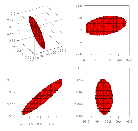
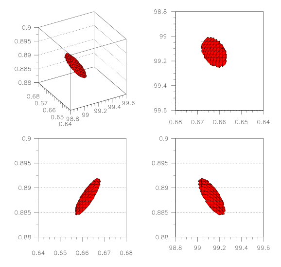
In fig. 3 the contour of $\Delta\chi^{2}=1$ is shown in the $M_{1},{\cos 2\Phi_{L}},\cos 2\Phi_{R}$ parameter space along with its three 2dim projections. The projection of the contours onto the axes determines 1$\sigma$ errors for each parameter.

Values obtained for $M_{1},{\cos 2\Phi_{L}},\cos 2\Phi_{R}$ together with $m_{\tilde{\chi}^{\pm}_{1}}$ can be inverted to derive the fundamental parameters $M_{2}$, $\mu$ and $\tan\beta$. At the same time masses of heavy chargino and neutralinos are predicted. As can be seen in table 5, the parameters $M_{1}$ and $M_{2}$ are determined at the level of a few per-mil, while $\mu$ is reconstructed within a few per-cent. Since the derived limits on $\tan\beta$ are asymmetric, we show the interval consistent with $\Delta\chi^{2}=1$.

Figure 4: The correlation between predicted values of $\mu$ and $m_{\tilde{\chi}^{0}_{4}}$ (left panel) and the allowed range of $\tan\beta$ and $m_{\tilde{\chi}^{0}_{4}}$ (right panel) from the analysis of the LC data.

The errors on the predicted masses of the heavy chargino/neutralinos, which in our SPS1a scenario are predominantly higgsinos, are strongly correlated with the error of $\mu$; the left panel of fig. 4 shows the correlation between $\mu$ and $m_{\tilde{\chi}^{0}_{4}}$. In the right panel of this figure a weaker correlation is observed between $\tan\beta$ and $m_{\tilde{\chi}^{0}_{4}}$ (or between $\tan\beta$ and $\mu$). Therefore, by providing $m_{\tilde{\chi}^{0}_{4}}$ from endpoint measurements [15], the LHC could considerably help to get a better accuracy on $\mu$. At the same time a better determination of $\tan\beta$ can be expected.

SUSY Parameters				Mass Predictions
$M_{1}$	$M_{2}$	$\mu$	$\tan\beta$	$m_{\tilde{\chi}^{\pm}_{2}}$	$m_{\tilde{\chi}^{0}_{3}}$	$m_{\tilde{\chi}^{0}_{4}}$
$99.1\pm 0.2$	$192.7\pm 0.6$	$352.8\pm 8.9$	$10.3\pm 1.5$	$378.8\pm 7.8$	$359.2\pm 8.6$	$378.2\pm 8.1$

Table 5: SUSY parameters with 1$\sigma$ errors derived from the analysis of the LC data collected at the first phase of operation. Shown are also the predictions for the heavier chargino/neutralino masses.

4 Combined strategy for the LHC and LC

4.1 LC data supplemented by ${\boldmath m_{\tilde{\chi}^{0}_{4}}}$ from the LHC

The LHC experiments will be able to measure the masses of several sparticles, as described in detail in [15]. In particular, the LHC will provide a first measurement of the masses of ${\tilde{\chi}}^{0}_{1}$, ${\tilde{\chi}}^{0}_{2}$ and ${\tilde{\chi}}^{0}_{4}$. The measurements of ${\tilde{\chi}}^{0}_{2}$ and ${\tilde{\chi}}^{0}_{4}$ are achieved through the study of the processes:

$$\tilde{\chi}^{0}_{i}\rightarrow\tilde{\ell}\ell\rightarrow\ell\ell{\tilde{\chi}}^{0}_{1}$$ (32)

where the index $i$ can be either 2 or 4. The invariant mass of the two leptons in the final state shows an abrupt edge, which can be expressed in terms of the masses of the relevant sparticles as

$$m_{l^{+}l^{-}}^{max}=m_{{\tilde{\chi}}^{0}_{i}}\sqrt{1-\frac{m^{2}_{\tilde{\ell}}}{m^{2}_{{\tilde{\chi}}^{0}_{i}}}}\sqrt{1-\frac{m^{2}_{{\tilde{\chi}}^{0}_{1}}}{m^{2}_{\tilde{\ell}}}}$$ (33)

If one only uses the LHC information, the achievable precision on $m_{{\tilde{\chi}}^{0}_{2}}$ and $m_{{\tilde{\chi}}^{0}_{4}}$ will be respectively of 4.5 and 5.1 GeV for an integrated luminosity of 300 fb^-1.

In the case of the ${\tilde{\chi}}^{0}_{4}$, which in the considered scenario is mainly higgsino, this information can be exploited at the LC to constrain the parameter $\mu$ with a better precision. If we include this improved precision on $m_{\tilde{\chi}^{0}_{4}}$ in the $\Delta\chi^{2}$ test of eq. (31), the resulting $\Delta\chi^{2}=1$ contours get modified and the achievable precision is improved, as shown in table 6.

SUSY Parameters				Mass Predictions
$M_{1}$	$M_{2}$	$\mu$	$\tan\beta$	$m_{\tilde{\chi}^{\pm}_{2}}$	$m_{\tilde{\chi}^{0}_{3}}$
$99.1\pm 0.2$	$192.7\pm 0.5$	$352.4\pm 4.5$	$10.2\pm 0.9$	$378.5\pm 4.1$	$358.8\pm 4.1$

Table 6: SUSY parameters with 1$\sigma$ errors derived from the analysis of the LC data collected at the first phase of operation and with $\delta m_{\tilde{\chi}^{0}_{4}}=5.1$ GeV from the LHC. Shown are also the predictions for the masses of $\tilde{\chi}^{\pm}_{2}$ and $\tilde{\chi}^{0}_{3}$.

4.2 Joint analysis of the LC and LHC data

From the consideration of eq. (33), one can see that the uncertainty on the LHC measurement of $m_{\tilde{\chi}^{0}_{2}}$ and $m_{\tilde{\chi}^{0}_{4}}$ depends both on the experimental error on the position of $m_{l^{+}l^{-}}^{max}$, and on the uncertainty on $m_{\tilde{\chi}^{0}_{1}}$ and $m_{\tilde{\ell}}$. The latter uncertainty, which for both masses is of 4.8 GeV, turns out to be the dominant contribution. A much higher precision can thus be achieved by inserting in eq. (33) the values for $m_{\tilde{\chi}^{0}_{1}}$, $m_{\tilde{e}_{R}}$ and $m_{\tilde{e}_{L}}$ which are measured at the LC with precisions respectively of 0.05, 0.05 and 0.2 GeV, table 1.

Figure 5: The $\Delta\chi^{2}=1$ contour in the $M_{1},{\cos 2\Phi_{L}},\cos 2\Phi_{R}$ parameter space, and its three 2dim projections, derived from the joint analysis of the LC data and LHC data.

With this input the precisions on the LHC+LC measurements of $m_{\tilde{\chi}^{0}_{2}}$ and $m_{\tilde{\chi}^{0}_{4}}$ become: $\delta m_{\tilde{\chi}^{0}_{2}}=0.08$ GeV and $\delta m_{\tilde{\chi}^{0}_{4}}=2.23$ GeV.

SUSY Parameters				Mass Predictions
$M_{1}$	$M_{2}$	$\mu$	$\tan\beta$	$m_{\tilde{\chi}^{\pm}_{2}}$	$m_{\tilde{\chi}^{0}_{3}}$
$99.1\pm 0.1$	$192.7\pm 0.3$	$352.4\pm 2.1$	$10.2\pm 0.6$	$378.5\pm 2.0$	$358.8\pm 2.1$

Table 7: SUSY parameters with 1$\sigma$ errors derived from the combined analysis of the LHC and LC data with $\delta m_{\tilde{\chi}^{0}_{2}}=0.08$ GeV and $\delta m_{\tilde{\chi}^{0}_{4}}=2.23$ GeV derived from the LHC when using the LC input of $\delta m_{\tilde{\chi}^{0}_{1}}=0.05$ GeV.

From the results of the $\Delta\chi^{2}$ test one can calculate the improvement in accuracy for the derived parameters by imposing the new mass constraints. The final results are shown in table 7. The accuracy for the parameters $\mu$ and particularly $\tan\beta$ is much better, as could be expected from fig. 4, where the allowed range of $\mu$ and $\tan\beta$ from the LC analysis is considerably reduced once the measured mass $m_{\tilde{\chi}^{0}_{4}}$ at the LHC is taken into account. In particular, the precision on $\tan\beta$ becomes better than from other SUSY sectors [14, 10].

5 Summary

We have worked out in a specific example, a mSUGRA scenario with rather high $\tan\beta=10$, how the combination of the results from the two accelerators, LHC and LC, allows a precise determination of the fundamental SUSY parameters without assuming a specific supersymmetry breaking scheme.

Measuring with high precision the masses of the expected lightest SUSY particles $\tilde{\chi}^{0}_{1}$, $\tilde{\chi}^{0}_{2}$, $\tilde{\chi}^{\pm}_{1}$ and their cross sections at the LC, and taking into account simulated mass measurement errors and corresponding uncertainties for the theoretical predictions, we could determine the fundamental SUSY parameters $M_{1}$, $M_{2}$, $\mu$ at tree level within a few percent, while $\tan\beta$ is estimated within $\sim$ 20 %. The masses of heavier chargino and neutralinos can also be predicted at a level of a few percent. The use of polarised beams at the LC is decisive for deriving unique solutions.

If the LC analysis is supplemented with the LHC measurement of the heavy neutralino mass, the errors on $\mu$ and $\tan\beta$ can be improved. However, the best results are obtained when first the LSP and slepton masses from the LC are fed to the LHC analyses to get a precise experimental determination of the ${\tilde{\chi}}^{0}_{2}$ and ${\tilde{\chi}}^{0}_{4}$ masses, which in turn are injected back to the analysis of the chargino/neutralino LC data. Such a combined strategy will provide in particular the precise measurement of the ${\tilde{\chi}}^{0}_{4}$ mass, the parameters $\mu$ with an accuracy at the $\leq O(1\%)$ level, and the error for $\tan\beta$ of the order of $\leq$ 10%, reaching a stage where radiative corrections become relevant in the electroweak sector and which will have to be taken into account in future fits [9].

Acknowledgments

The authors would like to thank G. Weiglein for motivating this project and for the coordination of the LHC/LC working group. We are indebted to G. Blair, U. Martyn and W. Porod for useful discussions and for providing the errors for simulated mass and cross section measurements at the LC. The work is supported in part by the European Commission 5-th Framework Contract HPRN-CT-2000-00149. JK was supported by the KBN Grant 2 P03B 040 24 (2003-2005).

Appendix

a) For the lightest chargino pair production, $\sigma^{\pm}\{11\}=\sigma(e^{-}(p_{1})e^{+}(p_{2})\to\tilde{\chi}^{+}_{1}(p_{3})\tilde{\chi}^{-}_{1}(p_{4}))$, the coefficients $c_{1},\ldots,c_{6}$ in eq. (12) are given by:

$$c_{1} = \int_{C}|Z|^{2}\{c_{LR}L^{2}f_{2}+c_{RL}R^{2}f_{1}\}$$

$$c_{2} = \int_{C}|Z|^{2}\{c_{LR}L^{2}(1-4L)(2f_{2}+f_{3})+c_{RL}R^{2}(1-4R)(2f_{1}+f_{3})\}$$

$$-\int_{C}G\tilde{N}4\{c_{LR}L(2f_{2}+f_{3})+c_{RL}R(2f_{1}+f_{3})\}-\int_{C}Re(Z)\tilde{N}c_{LR}Lf_{3}$$

$$c_{3} = \int_{C}|Z|^{2}(c_{LR}L^{2}f_{1}+c_{RL}R^{2}f_{2})-\int_{C}Z\tilde{N}2c_{LR}Lf_{1}+\int_{C}\tilde{N}^{2}c_{LR}f_{1}$$

$$c_{4} = \int_{C}|Z|^{2}(1-4L)\{c_{LR}L^{2}(2f_{1}+f_{3})+c_{RL}R^{2}(2f_{2}+f_{3})\}+\int_{C}\tilde{N}^{2}2c_{LR}f_{1}$$

$$+\int_{C}Re(Z)\tilde{N}c_{LR}L\{-4f_{1}-f_{3}+4L(2f_{1}+f_{3})\}+\int_{C}G\tilde{N}4c_{LR}(2f_{1}+f_{3})$$

$$-\int_{C}GRe(Z)4\{c_{LR}L(2f_{1}+f_{3})+c_{RL}R(2f_{2}+f_{3})\}$$

$$c_{5} = \int_{C}|Z|^{2}(c_{LR}L^{2}+c_{RL}R^{2})f_{3}-\int_{C}Re(Z)\tilde{N}c_{LR}Lf_{3}$$

$$c_{6} = \int_{C}|Z|^{2}\{c_{LR}L^{2}(1-8L)+c_{RL}R^{2}(1-8L)+16L^{2}(c_{LR}L^{2}+c_{RL}R^{2})\}(f_{1}+f_{2}+f_{3})$$

$$-\int_{C}Re(Z)\tilde{N}c_{LR}L(1-4L)(2f_{1}+f_{3})+\int_{C}G^{2}(c_{LR}+c_{RL})(f_{1}+f_{2}+f_{3})$$

$$-\int_{C}Re(Z)G8\{c_{RL}R+c_{LR}L(1-4L)\}(f_{1}+f_{2}+f_{3})+\int_{C}\tilde{N}^{2}c_{LR}f_{1}$$

$$+\int_{C}G\tilde{N}4c_{LR}(2f_{1}+f_{3})$$

where $\int_{C}=\frac{q_{\tilde{\chi}}}{E_{b}^{3}}\frac{1}{2\pi}\int{\rm d}\cos\theta$, $L=-\frac{1}{2}+\sin^{2}\theta_{W}$, $R=\sin^{2}\theta_{W}$, and

$$G = e^{2}/s,\quad Z=g^{2}/\cos^{2}\theta_{W}(s-m_{Z}^{2}+im_{Z}\Gamma_{Z}),\quad\tilde{N}=g^{2}/(t-m_{\tilde{\nu}_{e}}^{2})$$

denote the $\gamma$, $Z$ and $\tilde{\nu}_{e}$ propagators,

$$c_{LR} = (1-P(e^{-}))(1+P(e^{+})),\quad c_{RL}=(1+P(e^{-}))(1-P(e^{+}))$$

are the beam polarisation factors, and

$$f_{1}=(p_{1}p_{4})(p_{2}p_{3}),\quad f_{2}=(p_{1}p_{3})(p_{2}p_{4}),\quad f_{3}=s\,m^{2}_{\tilde{\chi}^{\pm}_{i}}/2$$

are the pure kinematic coefficients.

b) The coefficients $a_{kl}$ ($k=0,2,4,6$, $l=1,2,3$), which appear in eqns. (20),(21) and (22), are invariants of the matrix ${\cal M}_{N}{\cal M}_{N}^{T}$. They can be expressed as functions of the parameters $M_{2}$, $\mu$, $\tan\beta$ in the following way:

$$a_{63} = M_{2}^{2}+2(\mu^{2}+m_{Z}^{2})$$

$$a_{41} = M_{2}^{2}+2(\mu^{2}+m_{Z}^{2}\cos^{2}\theta_{W})$$

$$a_{42} = -2\mu m_{Z}^{2}\sin 2\beta\sin^{2}\theta_{W}$$

$$a_{43} = 2\mu^{2}M_{2}^{2}+(\mu^{2}+m_{Z}^{2})^{2}-2m_{Z}^{2}\mu M_{2}\sin 2\beta\cos^{2}\theta_{W}+2m_{Z}^{2}M_{2}^{2}\sin^{2}\theta_{W}$$

$$a_{21} = \mu^{4}+2\mu^{2}M_{2}^{2}+2m_{Z}^{2}\mu^{2}\cos^{2}\theta_{W}+m_{Z}^{4}\cos^{2}\theta_{W}-2m_{Z}^{2}M_{2}\mu\sin 2\beta\cos^{2}\theta_{W}$$

$$a_{22} = 2[m_{Z}^{4}M_{2}\sin^{2}\theta_{W}\cos^{2}\theta_{W}-m_{Z}^{2}\mu^{3}\sin^{2}\theta_{W}\sin 2\beta-m_{Z}^{2}\mu M_{2}^{2}\sin^{2}\theta_{W}\sin 2\beta]$$

$$a_{23} = \mu^{4}M_{2}^{2}+m_{Z}^{4}\mu^{2}\sin^{2}2\beta+2m_{Z}^{2}\mu^{2}M_{2}^{2}\sin^{2}\theta_{W}-2m_{Z}^{2}M_{2}\mu^{3}\cos^{2}\theta_{W}\sin 2\beta+m_{Z}^{4}M_{2}^{2}\sin^{4}\theta_{W}$$

$$a_{01} = \mu^{4}M_{2}^{2}+m_{Z}^{4}\mu^{2}\cos^{4}\theta_{W}\sin^{2}2\beta-2m_{Z}^{2}\mu^{3}M_{2}\cos^{2}\theta_{W}\sin 2\beta$$

$$a_{02} = 2m_{Z}^{4}\mu^{2}M_{2}\sin^{2}\theta_{W}\cos^{2}\theta_{W}\sin^{2}2\beta-2m_{Z}^{2}\mu^{3}M_{2}^{2}\sin^{2}\theta_{W}\sin 2\beta$$

$$a_{03} = m_{Z}^{4}\mu^{2}M_{2}^{2}\sin^{4}\theta_{W}\sin^{2}2\beta$$

References

- [1] A summary of current LC studies can be found e.g. in J. Kalinowski, arXiv:hep-ph/0309235, and references therein.
- [2] T. Tsukamoto, K. Fujii, H. Murayama, M. Yamaguchi and Y. Okada, Phys. Rev. D 51 (1995) 3153. J. L. Feng, M. E. Peskin, H. Murayama and X. Tata, Phys. Rev. D 52 (1995) 1418 [arXiv:hep-ph/9502260].
- [3] S. Y. Choi, J. Kalinowski, G. Moortgat-Pick and P. M. Zerwas, Eur. Phys. J. C 22 (2001) 563 [arXiv:hep-ph/0108117]; S. Y. Choi, J. Kalinowski, G. Moortgat-Pick and P. M. Zerwas, Eur. Phys. J. C 23 (2002) 769 [arXiv:hep-ph/0202039].
- [4] B. C. Allanach et al., Eur. Phys. J. C 25 (2002) 113 [eConf C010630 (2001) P125] [arXiv:hep-ph/0202233]; N. Ghodbane and H.-U. Martyn, hep-ph/0201233; see also the webpage: http://www.cpt.dur.ac.uk/ georg/sps/.
- [5] H. E. Haber and G. L. Kane, Phys. Rep. 117 (1985) 75.
- [6] S. Y. Choi, A. Djouadi, M. Guchait, J. Kalinowski, H. S. Song and P. M. Zerwas, Eur. Phys. J. C 14 (2000) 535 [arXiv:hep-ph/0002033]; S. Y. Choi, A. Djouadi, H. K. Dreiner, J. Kalinowski and P. M. Zerwas, Eur. Phys. J. C 7 (1999) 123 [arXiv:hep-ph/9806279].
- [7] G. Moortgat-Pick, A. Bartl, H. Fraas and W. Majerotto, arXiv:hep-ph/0002253.
- [8] S. Ambrosanio, B. Mele, G. Montagna, O. Nicrosini and F. Piccinini, Nucl. Phys. B 478 (1996) 46 [arXiv:hep-ph/9601292].
- [9] T. Blank and W. Hollik, hep-ph/0011092; H. Eberl, M. Kincel, W. Majerotto and Y. Yamada, hep-ph/0104109. T. Fritzsche and W. Hollik, Eur. Phys. J. C 24 (2002) 619 [arXiv:hep-ph/0203159].
- [10] E. Boos, G. Moortgat-Pick, H. U. Martyn, M. Sachwitz and A. Vologdin, arXiv:hep-ph/0211040; E. Boos, H. U. Martyn, G. Moortgat-Pick, M. Sachwitz, A. Sherstnev and P. M. Zerwas, Eur. Phys. J. C 30 (2003) 395 [arXiv:hep-ph/0303110].
- [11] H.U. Martyn, talk given at the ECFA/DESY Linear Collider workshop, Prague, November 2002, http://www-hep2.fzu.cz/ecfadesy/Talks/SUSY/, and LC-note LC-PHSM-2003-071. M. Dima et al., Phys. Rev. D 65 (2002) 071701.
- [12] M. Ball, diploma thesis, University of Hamburg, January 2003, http://www-flc.desy.de/thesis/diplom.2002.ball.ps.gz; see also talk by K. Desch at the ECFA/DESY Linear Collider workshop, Prague, November 2002, http://www-hep2.fzu.cz/ecfadesy/Talks/SUSY/.
- [13] ’Polarisation Write-Up: Beam Polarisation at a future Linear Collider’, working group document by the polarisation ‘POWER working group’, G. Moortgat-Pick et al., in preparation, further details: http://www.ippp.durham.ac.uk/ gudrid/power.
- [14] H. Baer, C. H. Chen, M. Drees, F. Paige and X. Tata, Phys. Rev. D 59 (1999) 055014 [arXiv:hep-ph/9809223]; J. L. Feng and T. Moroi, Nucl. Phys. Proc. Suppl. 62 (1998) 108 [arXiv:hep-ph/9707494]; V. D. Barger, T. Han and J. Jiang, Phys. Rev. D 63 (2001) 075002 [arXiv:hep-ph/0006223]; J. F. Gunion, T. Han, J. Jiang and A. Sopczak, hep-ph/0212151.
- [15] B.K. Gjelsten, E. Lytken, D. Miller, P. Osland, G. Polesello, contribution in the LHC/LC working group document, see also http://www.ippp.dur.ac.uk/ georg/lhclc/.