Virtual- and bremsstrahlung corrections to $\bm{b\rightarrow d\,\ell^{+}\ell^{-}}$ in the standard model

Abstract

We present the calculation of the virtual- and bremsstrahlung corrections of ${\cal O}(\alpha_{s})$ to the matrix elements $\langle d\,\ell^{+}\ell^{-}|O_{i}|b\rangle$. This is the missing piece in the full next-to-next-to-leading logarithmic (NNLL) results for various observables associated with the process $B\to X_{d}\ell^{+}\ell^{-}$, like the branching ratio, the CP-rate asymmetry and the forward-backward asymmetry. This paper is an extension of analogous calculations done by some of us for the process $B\to X_{s}\ell^{+}\ell^{-}$. As the contributions of the diagrams induced by the four-quark operators $O_{1}^{u}$ and $O_{2}^{u}$ with a $u$-quark running in the quark loop are strongly CKM suppressed, they were omitted in the analysis of $B\to X_{s}\ell^{+}\ell^{-}$. This is no longer possible for $B\to X_{d}\ell^{+}\ell^{-}$, as the corresponding contributions are not suppressed. The main new work therefore consists of calculating the ${\cal O}(\alpha_{s})$ corrections to $\langle d\,\ell^{+}\ell^{-}|O_{1,2}^{u}|b\rangle$. In this paper we restrict ourselves to the range $0.05\leq s/m_{b}^{2}\leq 0.25$ ($s$ is the invariant mass of the lepton pair), which lies above the $\rho$- and $\omega$-resonances and below the $J/\psi$-resonance. We present the analytic results for the mentioned observables related to the process $B\to X_{d}\ell^{+}\ell^{-}$ as expansions in the small parameters $\hat{s}=s/m_{b}^{2}$, $z=m_{c}^{2}/m_{b}^{2}$ and $s/(4\,m_{c}^{2})$. In the phenomenological analysis at the end of the paper we discuss the impact of the NNLL corrections on the observables mentioned above.

I Introduction

It is well-known that various observables associated with inclusive rare $B$-decays like $B\to X_{s,d}\gamma$ and $B\to X_{s,d}\ell^{+}\ell^{-}$ sensitively depend on potential new physics contributions. But even in the absence of new physics these observables are important, because they provide checks on the one-loop structure of the Standard Model (SM) theory and can be used to gain information on the Cabibbo-Kobayashi-Maskawa (CKM) matrix elements $V_{ts}$ and $V_{td}$, which are difficult to measure directly.

At present, a lot of data already exists on ${\rm BR}(B\to X_{s}\gamma)$ [1, 2, 3, 4, 5, 6, 7] and on ${\rm BR}(B\to X_{s}\ell^{+}\ell^{-})$ [8, 9, 10] and it is expected that in the future also data on the CKM suppressed counterparts, i.e. on ${\rm BR}(B\to X_{d}\gamma)$ and on ${\rm BR}(B\to X_{d}\ell^{+}\ell^{-})$ will become available. The same holds for experimental information on additional observables, like CP-rate asymmetries or forward-backward asymmetries in the decays $B\to X_{s,d}\ell^{+}\ell^{-}$.

In order to fully exploit and interpret the experimental data, it is obvious that precise calculations in the SM (or certain extensions thereof) are needed. The main problem in the theoretical description of the decay $B\to X_{s}\ell^{+}\ell^{-}$ is due to the long-distance contributions induced by $\bar{c}c$ resonant states and in principle also by $\bar{u}u$ resonant states. The latter are, however, strongly CKM suppressed. This suppression is not present in the case of $B\to X_{d}\ell^{+}\ell^{-}$, as the CKM factors involved in the contributions from $\bar{c}c$ and $\bar{u}u$ resonant states are of the same order. When the invariant mass $\sqrt{s}$ of the lepton pair is close to the mass of a resonance, only model dependent predictions for such long distance contributions are available at present. It is therefore unclear whether the theoretical uncertainty can be reduced to less than $\pm 20\%$ when integrating over these domains [11].

However, restricting $\sqrt{s}$ to a region below the $\bar{c}c$ resonances, the long distance effects in $B\to X_{s}\ell^{+}\ell^{-}$ are under control. The same is true for $B\to X_{d}\ell^{+}\ell^{-}$ when choosing a region of $\sqrt{s}$ which is below the $J/\psi$- and above the $\rho,\omega$-resonance regions. It turns out that in those ranges of $\sqrt{s}$ the corrections to the pure perturbative picture can be analyzed within the heavy quark effective theory (HQET). In particular, all available studies indicate that for the region $0.05<\hat{s}=s/m_{b}^{2}<0.25$ the non-perturbative effects are below 10$\%$ [12, 13, 14, 15, 16, 17]. Consequently, observables like differential decay rates, forward-backward asymmetries and CP-rate asymmetries for $B\to X_{s,d}\ell^{+}\ell^{-}$ can be precisely predicted in this region of $\sqrt{s}$ using renormalization group improved perturbation theory. It was pointed out in the literature that the differential decay rate and the forward-backward asymmetry in $B\to X_{s}\ell^{+}\ell^{-}$ are particularly sensitive to new physics in this kinematical window [18, 19, 20].

In the context of the SM there exist computations of next-to-leading logarithmic (NLL) QCD corrections to the branching ratios for $B\to X_{s}\gamma$ [21, 22, 23, 24, 25, 26, 27, 28] and $B\to X_{d}\gamma$ and the corresponding CP-rate asymmetries [29, 30, 31]. Next-to-next-to-leading logarithmic (NNLL) QCD corrections to the branching ratio [32, 33, 34, 35, 36] and the forward-backward asymmetry in $B\to X_{s}\ell^{+}\ell^{-}$ are also available [37, 38, 39, 40]. For a recent review see e.g. [41].

The corresponding NNLL results for the process $B\to X_{d}\ell^{+}\ell^{-}$ are missing, however. The aim of the present paper is to close this gap. The main difference between the calculations for $B\to X_{s}\ell^{+}\ell^{-}$ and $B\to X_{d}\ell^{+}\ell^{-}$ lies in the contributions of the current-current operators. In the existing NNLL calculations of $B\to X_{s}\ell^{+}\ell^{-}$ only those associated with $O_{1}^{c}$ and $O_{2}^{c}$ were included at the two-loop level because those induced by $O_{1}^{u}$ and $O_{2}^{u}$ are strongly CKM suppressed (see Section II for the definition of the operators $O_{1,2}^{u,c}$). For $B\to X_{d}\ell^{+}\ell^{-}$ the contributions generated by $O_{1}^{u}$ and $O_{2}^{u}$ are no longer CKM suppressed and have to be taken into account as well. At first sight, it seems that the two-loop matrix elements of $O_{1}^{u}$ and $O_{2}^{u}$ can be straightforwardly obtained from those of $O_{1}^{c}$ and $O_{2}^{c}$ by simply taking the limit $m_{c}\to 0$. This is, however, not possible for some of the diagrams in Fig. 1, because the two-loop matrix elements of $O_{1}^{c}$ and $O_{2}^{c}$ were derived by doing various expansions. In particular, one of the expansion parameters is $s/(4m_{c}^{2})$, which is formally $\ll 1$ when restricting $\sqrt{s}$ to the window discussed above. Obviously, the analogous quantity for the $u$-quark contribution, $s/(4m_{u}^{2})$, cannot be used as an expansion parameter, which implies that genuinely new calculations for the $u$-quark contributions are needed. As discussed in Section III, the calculations of certain diagrams associated with $O_{1,2}^{u}$ are even more involved than those associated with $O_{1,2}^{c}$. To derive the new results, we used dimension-shifting techniques in order to reduce certain tensor integrals to scalar ones and integration-by-parts techniques to further simplify the scalar integrals [42, 43].

As the main emphasis of this paper is the derivation of the matrix elements $\langle d\,\ell^{+}\ell^{-}|O_{1,2}^{u}|b\rangle$ at order $\alpha_{s}$, we keep the phenomenological analysis relatively short. In particular, we do not take into account power corrections, but merely illustrate how the NNLL contributions modify the scale dependences of the branching ratio, the forward-backward asymmetry and the CP-rate asymmetry. A more detailed phenomenology, including power corrections, will be presented elsewhere.

The paper is organized as follows: In Section II we present the effective Hamiltonian for the decay $b\to X_{d}\ell^{+}\ell^{-}$. Section III is devoted to the virtual ${\cal O}(\alpha_{s})$ corrections to the operators $O_{1}^{u,c}$ and $O_{2}^{u,c}$. Subsequently, Section IV presents the corresponding contributions to the form factors of the operators $O_{7},\,O_{8},\,O_{9}$ and $O_{10}$. With these results at hand, we discuss in Section V the corrections to the decay width of $B\to X_{d}\ell^{+}\ell^{-}$. In Section VI we show some applications of our results. A summary of the paper is presented in Section VII. The appendices contain technical details about the performed calculation: Appendix A explains the dimension-shifting and integration-by-parts techniques. These techniques are then applied to the calculation of diagrams 1d), which is presented in Appendix B. Appendix C outlines a procedure on how to calculate the evolution matrix for the Wilson coefficients as a power series in $\alpha_{s}$. Appendix D contains one-loop matrix elements needed in the calculation of the counterterms. Finally, in Appendix E we present the results for those bremsstrahlung contributions which are free of infrared and collinear divergences.

II Effective Hamiltonian

The appropriate framework for studying QCD corrections to rare $B$-decays in a systematic way is the effective Hamiltonian technique. For the specific decay channels $B\rightarrow X_{s}\ell^{+}\ell^{-}$ and $B\to X_{d}\ell^{+}\ell^{-}$ ($\ell=\mu$, $e$), the effective Hamiltonian is derived by integrating out the $t$-quark, the $W$-boson and the $Z^{0}$-boson. In the process $B\to X_{s}\ell^{+}\ell^{-}$, the appearing CKM combinations are $\lambda_{u}$, $\lambda_{c}$ and $\lambda_{t}$, where $\lambda_{i}=V_{ib}V_{is}^{*}$. Since $|\lambda_{u}|$ is much smaller than $|\lambda_{c}|$ and $|\lambda_{t}|$, it is a safe approximation to set $\lambda_{u}$ equal to zero. Using then the unitarity properties of the CKM matrix, the CKM dependence of the Hamiltonian can be written as a global factor $\lambda_{t}$. In the case of $B\to X_{d}\ell^{+}\ell^{-}$, all three quantities $\xi_{i}=V_{ib}V_{id}^{*}$ ($i=u,c,t$) are of the same order of magnitude. Therefore, as no approximation is possible, the CKM dependence does not globally factorize. The effective Hamiltonian reads

$${\cal H}_{\text{eff}}=\frac{4\,G_{F}}{\sqrt{2}}\left[\sum_{i=1}^{2}C_{i}(\xi_{c}\,O_{i}^{c}+\xi_{u}O_{i}^{u})-\xi_{t}\sum_{i=3}^{10}C_{i}\,O_{i}\right]\,.$$ (1)

We choose the operator basis according to [32]:

$$\begin{array}[]{rclrcl}O_{1}^{u}&=&(\bar{d}_{L}\gamma_{\mu}T^{a}u_{L})(\bar{u}_{L}\gamma^{\mu}T^{a}b_{L}),&O_{2}^{u}&=&(\bar{d}_{L}\gamma_{\mu}u_{L})(\bar{u}_{L}\gamma^{\mu}b_{L}),\vspace{0.2cm}\\ \vspace{0.3cm}O_{1}^{c}&=&(\bar{d}_{L}\gamma_{\mu}T^{a}c_{L})(\bar{c}_{L}\gamma^{\mu}T^{a}b_{L}),&O_{2}^{c}&=&(\bar{d}_{L}\gamma_{\mu}c_{L})(\bar{c}_{L}\gamma^{\mu}b_{L}),\\ \vspace{0.2cm}O_{3}&=&(\bar{d}_{L}\gamma_{\mu}b_{L})\sum_{q}(\bar{q}\gamma^{\mu}q),&O_{4}&=&(\bar{d}_{L}\gamma_{\mu}T^{a}b_{L})\sum_{q}(\bar{q}\gamma^{\mu}T^{a}q),\\ \vspace{0.2cm}O_{5}&=&(\bar{d}_{L}\gamma_{\mu}\gamma_{\nu}\gamma_{\rho}b_{L})\sum_{q}(\bar{q}\gamma^{\mu}\gamma^{\nu}\gamma^{\rho}q),&O_{6}&=&(\bar{d}_{L}\gamma_{\mu}\gamma_{\nu}\gamma_{\rho}T^{a}b_{L})\sum_{q}(\bar{q}\gamma^{\mu}\gamma^{\nu}\gamma^{\rho}T^{a}q),\\ \vspace{0.2cm}O_{7}&=&\frac{e}{g_{s}^{2}}m_{b}(\bar{d}_{L}\sigma^{\mu\nu}b_{R})F_{\mu\nu},&O_{8}&=&\frac{1}{g_{s}}m_{b}(\bar{d}_{L}\sigma^{\mu\nu}T^{a}b_{R})G_{\mu\nu}^{a},\\ \vspace{0.2cm}O_{9}&=&\frac{e^{2}}{g_{s}^{2}}(\bar{d}_{L}\gamma_{\mu}b_{L})\sum_{\ell}(\bar{\ell}\gamma^{\mu}\ell),&O_{10}&=&\frac{e^{2}}{g_{s}^{2}}(\bar{d}_{L}\gamma_{\mu}b_{L})\sum_{\ell}(\bar{\ell}\gamma^{\mu}\gamma_{5}\ell),\end{array}$$ (2)

where the subscripts $L$ and $R$ refer to left- and right-handed components of the fermion fields, respectively.

The factors $1/g_{s}^{2}$ in the definition of the operators $O_{7}$, $O_{9}$ and $O_{10}$ as well as the factor $1/g_{s}$ present in $O_{8}$ have been chosen by Misiak [44] in order to simplify the organization of the calculation. With these definitions, the one-loop anomalous dimensions [needed for a leading logarithmic (LL) calculation] of the operators $O_{i}$ are all proportional to $g_{s}^{2}$, while two-loop anomalous dimensions [needed for a next-to-leading logarithmic (NLL) calculation] are proportional to $g_{s}^{4}$, etc.

After this important remark we now outline the principal steps which lead to a LL, NLL, and a NNLL prediction for the decay amplitude for $b\to d\,\ell^{+}\ell^{-}$:

1. A matching calculation between the full SM theory and the effective theory has to be performed in order to determine the Wilson coefficients $C_{i}$ at the high scale $\mu_{W}\sim m_{W},m_{t}$. At this scale, the coefficients can be worked out in fixed order perturbation theory, i.e. they can be expanded in $g_{s}^{2}$:

   $$C_{i}(\mu_{W})=C_{i}^{(0)}(\mu_{W})+\frac{g_{s}^{2}}{16\pi^{2}}C_{i}^{(1)}(\mu_{W})+\frac{g_{s}^{4}}{(16\pi^{2})^{2}}C_{i}^{(2)}(\mu_{W})+{\cal O}(g_{s}^{6})\,.$$ (3)

   At LL order, only $C_{i}^{(0)}$ are needed, at NLL order also $C_{i}^{(1)}$, etc. The coefficient $C_{7}^{(2)}$ was worked out in Refs. [23, 24, 25], while $C_{9}^{(2)}$ and $C_{10}^{(2)}$ were calculated in Ref. [32].

2. The renormalization group equation (RGE) has to be solved in order to get the Wilson coefficients at the low scale $\mu_{b}\sim m_{b}$. For this RGE step the anomalous dimension matrix $\gamma(\alpha_{\text{s}})$, which can be expanded as

   $$\gamma(\alpha_{\text{s}})=\gamma^{(0)}\frac{\alpha_{\text{s}}}{4\pi}+\gamma^{(1)}\left(\frac{\alpha_{\text{s}}}{4\pi}\right)^{2}+\gamma^{(2)}\left(\frac{\alpha_{\text{s}}}{4\pi}\right)^{3}+\ldots\,,$$ (4)

   is required up to the term proportional to $\gamma^{(2)}$ when aiming at a NNLL calculation. After the matching step and the RGE evolution, the Wilson coefficients $C_{i}(\mu_{b})$ can be decomposed into a LL, NLL and NNLL part according to

   $$C_{i}(\mu_{b})=C_{i}^{(0)}(\mu_{b})+\frac{g_{s}^{2}(\mu_{b})}{16\pi^{2}}C_{i}^{(1)}(\mu_{b})+\frac{g_{s}^{4}(\mu_{b})}{(16\pi^{2})^{2}}C_{i}^{(2)}(\mu_{b})+{\cal O}(g_{s}^{6})\,.$$ (5)

   We stress at this point that the entries in $\gamma^{(2)}$ which describe the three-loop mixings of the four-quark operators $O_{1}-O_{6}$ into the operator $O_{9}$ have been calculated only recently [33]. In order to include the impact of these new ingredients on the Wilson coefficient $C_{9}(\mu_{b})$, we had to reanalyze the RGE step. In Appendix C, we derive a practical formula for the evolution matrix $U(\mu_{b},\mu_{W})$ at NNLL order, generalizing existing formulas at NLL order (see e.g. [45]).

3. In order to get the decay amplitude, the matrix elements $\langle d\,\ell^{+}\ell^{-}|O_{i}(\mu_{b})|b\rangle$ have to be calculated. At LL precision, only the operator $O_{9}$ contributes, as this operator is the only one which at the same time has a Wilson coefficient starting at lowest order and an explicit $1/g_{s}^{2}$ factor in the definition. Hence, at NLL precision, QCD corrections (virtual and bremsstrahlung) to the matrix element of $O_{9}$ are needed. They have been calculated in Refs. [44, 46]. At NLL precision, also the other operators start contributing, viz. $O_{7}(\mu_{b})$ and $O_{10}(\mu_{b})$ contribute at tree-level and the four-quark operators $O_{1},...,O_{6}$ at one-loop level. Accordingly, QCD corrections to the latter matrix elements are needed for a NNLL prediction of the decay amplitude.

The formally leading term $\sim(1/g_{s}^{2})C_{9}^{(0)}(\mu_{b})$ to the amplitude for $b\to d\,\ell^{+}\ell^{-}$ is smaller than the NLL term $\sim(1/g_{s}^{2})[g_{s}^{2}/(16\pi^{2})]\,C_{9}^{(1)}(\mu_{b})$ [47]. We adapt our systematics to the numerical situation and treat the sum of these two terms as a NLL contribution. This is, admittedly some abuse of language, because the decay amplitude then starts out with a term which is called NLL.

As pointed out in step 3), ${\cal O}(\alpha_{s})$ QCD corrections to the matrix elements $\langle d\,\ell^{+}\ell^{-}|O_{i}(\mu_{b})|b\rangle$ have to be calculated in order to obtain the NNLL prediction for the decay amplitude. In the present paper we systematically evaluate virtual corrections of order $\alpha_{s}$ to the matrix elements of $O_{1}$, $O_{2}$, $O_{7}$, $O_{8}$, $O_{9}$ and $O_{10}$. As the Wilson coefficients of the gluonic penguin operators $O_{3},...,O_{6}$ are much smaller than those of $O_{1}$ and $O_{2}$, we neglect QCD corrections to their matrix elements. We also systematically include gluon bremsstrahlung corrections to the matrix elements of the operators just mentioned. Some of these contributions contain infrared and collinear singularities, which are canceled when combined with the virtual corrections.

III Virtual $\bm{{\cal O}(\alpha_{s})}$ Corrections to the matrix elements $\bm{\langle d\,\ell^{+}\ell^{-}|O_{1,2}^{u,c}|b\rangle}$

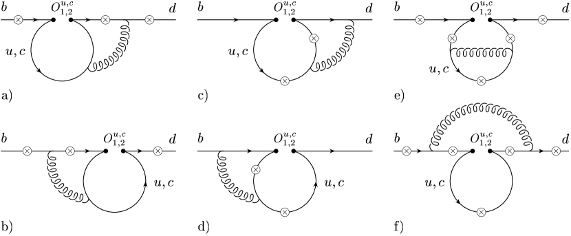
Figure 1: Complete list of two-loop Feynman diagrams for $b\to d\,\gamma^{*}$ associated with the operators $O_{1}^{u,c}$ and $O_{2}^{u,c}$. The fermions ($b$-, $d$-, $u$- and $c$-quarks) are represented by solid lines, whereas the curly lines represent gluons. The circle-crosses denote the possible locations where the virtual photon (which then splits into a lepton pair) is emitted.

In this section we present the calculation of the virtual ${\cal O}(\alpha_{s})$ corrections to the matrix elements of the current-current operators $O_{1}^{u,c}$ and $O_{2}^{u,c}$. Using the naive dimensional regularization scheme (NDR) in $d=4-2\,\epsilon$ dimensions, both ultraviolet and infrared singularities show up as $1/\epsilon^{n}$ poles ($n=1,2$). The ultraviolet singularities cancel after including the counterterms. Collinear singularities are regularized by retaining a finite down quark mass $m_{d}$. They are canceled together with the infrared singularities at the level of the decay width when taking the bremsstrahlung process $b\to d\,\ell^{+}\ell^{-}g$ into account. We use the $\overline{\text{MS}}$ renormalization scheme, i.e. we introduce the renormalization scale in the form $\overline{\mu}^{\,2}=\mu^{2}\exp(\gamma_{E})/(4\,\pi)$ followed by minimal subtraction. The precise definition of the evanescent operators, which is necessary to fully specify the renormalization scheme, will be given later.

Gauge invariance implies that the QCD corrected matrix elements of the operators $O_{i}^{q}$ can be written as

$$\langle d\,\ell^{+}\ell^{-}|O_{i}^{q}|b\rangle=\hat{F}_{i,q}^{(9)}\langle O_{9}\rangle_{\text{tree}}+\hat{F}_{i,q}^{(7)}\langle O_{7}\rangle_{\text{tree}}\quad(i=1,2;\,\,q=u,c)\,,$$ (6)

where $\langle O_{9}\rangle_{\text{tree}}$ and $\langle O_{7}\rangle_{\text{tree}}$ are the tree-level matrix elements of $O_{9}$ and $O_{7}$, respectively. Equivalently, we may write

$$\langle d\,\ell^{+}\ell^{-}|O_{i}^{q}|b\rangle=-\frac{\alpha_{s}}{4\,\pi}\,\left[F_{i,q}^{(9)}\langle\widetilde{O}_{9}\rangle_{\text{tree}}+F_{i,q}^{(7)}\langle\widetilde{O}_{7}\rangle_{\text{tree}}\right],$$ (7)

where the operators $\widetilde{O}_{7}$ and $\widetilde{O}_{9}$ are defined as

$$\widetilde{O}_{7}=\frac{\alpha_{s}}{4\,\pi}\,O_{7},\quad\widetilde{O}_{9}=\frac{\alpha_{s}}{4\,\pi}\,O_{9}.$$ (8)

We present the final results for the QCD corrected matrix elements in the form of Eq. (7). The full set of the diagrams contributing at ${\cal O}(\alpha_{s})$ to the matrix elements

$$M_{i}^{q}=\langle d\,\ell^{+}\ell^{-}|O_{i}^{q}|b\rangle$$ (9)

is shown in Fig. 1. As indicated, the diagrams associated with $O_{1}^{u,c}$ and $O_{2}^{u,c}$ are topologically identical. They differ only in the color structure. While the matrix elements of the operator $O_{2}^{u,c}$ all involve the color structure

$$\sum_{a}T^{a}T^{a}=C_{F}{\bf 1},\quad C_{F}=\frac{N_{c}^{2}-1}{2\,N_{c}}\,,$$

there are two possible color structures for the corresponding diagrams of $O_{1}^{u,c}$, viz

$$\tau_{1}=\sum_{a,b}T^{a}T^{b}T^{a}T^{b}\quad\text{and}\quad\tau_{2}=\sum_{a,b}T^{a}T^{b}T^{b}T^{a}.$$

The structure $\tau_{1}$ appears in diagrams 1a)-d), and $\tau_{2}$ enters diagrams 1e) and 1f). Using the relation

$$\sum_{a}\,T^{a}_{\alpha\beta}T^{a}_{\gamma\delta}=-\frac{1}{2\,N_{c}}\,\delta_{\alpha\beta}\delta_{\gamma\delta}+\frac{1}{2}\,\delta_{\alpha\delta}\delta_{\beta\gamma},$$

we find that $\tau_{1}=C_{\tau_{1}}{\bf 1}$ and $\tau_{2}=C_{\tau_{2}}{\bf 1}$, with

$$C_{\tau_{1}}=-\frac{N_{c}^{2}-1}{4\,N_{c}^{2}}\quad\text{and}\quad C_{\tau_{2}}=\frac{\left(N_{c}^{2}-1\right)^{2}}{4\,N_{c}^{2}}\,.$$

Inserting $N_{c}=3$, the color factors are $C_{F}=\frac{4}{3},C_{\tau_{1}}=-\frac{2}{9}$ and $C_{\tau_{2}}=\frac{16}{9}$. The contributions from $O_{1}^{u,c}$ are obtained by multiplying those from $O_{2}^{u,c}$ by the appropriate factors, i.e. by $C_{\tau_{1}}/C_{F}=-\frac{1}{6}$ and $C_{\tau_{2}}/C_{F}=\frac{4}{3}$, respectively. As the renormalized ${\cal O}(\alpha_{s})$ contributions of the operators $O_{1}^{c}$ and $O_{2}^{c}$ are discussed in detail in Ref. [34], we only discuss the calculations of the contributions from $O_{1}^{u}$ and $O_{2}^{u}$ to the individual form factors.

The rest of this section is organized as follows: We discuss the calculations of the diagrams 1a)-e) for the operators $O_{1,2}^{u}$. Notice that all results are given as an expansion in the small quantity $\hat{s}=s/m_{b}^{2}$, where $s$ is the invariant mass squared of the lepton pair, and that we keep only terms up to ${\cal O}(\hat{s}^{3})$. After deriving the counterterms that cancel the divergences of the diagrams mentioned above, we present the renormalized contributions to the form factors. We postpone the discussion of diagrams 1f) as it turns out to be more convenient to take them into account when discussing the virtual corrections to $O_{9}$.

III.1 Diagrams 1a) and b)

The calculation of the contributions to $F_{2,u}^{(7)}$ and $F_{2,u}^{(9)}$ from the diagrams in Figs. 1a) and 1b) opposes no difficulties, as it can be performed by using the Mellin-Barnes approach [48]. Alternatively, one may get the results directly from the corresponding form factors of the $b\to s\,\ell^{+}\ell^{-}$ transition by taking the limit $m_{c}\to 0$. The form factors associated with the diagrams in Fig. 1a) are given by

$$F_{2,u}^{(9)}[a]=C_{F}\cdot\Bigg{[} -\frac{2}{27\,\epsilon^{2}}+\left(\frac{1}{\epsilon}+4\,L_{\mu}\right)\left(-\frac{19}{81}+\frac{4}{27}\,L_{s}-\frac{4}{27}\,i\pi\right)-\frac{8}{27\,\epsilon}\,L_{\mu}$$

$$-\frac{16}{27}\,L_{\mu}^{2}+\left(-\frac{463}{486}-\frac{38\,i\pi}{81}+\frac{5\,\pi^{2}}{27}\right)-\frac{4}{27}\,\hat{s}+\left(-\frac{1}{27}-\frac{2}{27}\,L_{s}\right)\hat{s}^{2}$$

$$+\left(-\frac{4}{243}-\frac{8}{81}\,L_{s}\right)\hat{s}^{3}+\frac{26}{81}\,L_{s}+\frac{8}{27}\,i\pi\,L_{s}-\frac{2}{27}\,L_{s}^{2}\Bigg{]},$$ (10)

$$F_{2,u}^{(7)}[a]=C_{F}\cdot\Bigg{[} \frac{1}{27}\left(\frac{1}{\epsilon}+4\,L_{\mu}\right)+\frac{37}{162}+\frac{2}{27}\,i\pi+\frac{2}{27}\,\hat{s}\left(1+\hat{s}+\hat{s}^{2}\right)L_{s}\Bigg{]},$$

where

$$L_{s}=\ln(\hat{s})\quad\text{and}\quad L_{\mu}=\ln\!\left(\!\frac{\mu}{m_{b}}\right)\,.$$

For the sum of the diagrams in Fig. 1b) we find

$$F_{2,u}^{(9)}[b]=C_{F}\cdot\Bigg{[} -\frac{2}{27\,\epsilon^{2}}+\left(\frac{1}{\epsilon}+4\,L_{\mu}\right)\left(\frac{1}{81}-\frac{4}{135}\,\hat{s}-\frac{1}{315}\,\hat{s}^{2}-\frac{4}{8505}\,\hat{s}^{3}\right)-\frac{8}{27\,\epsilon}\,L_{\mu}$$

$$-\frac{16}{27}\,L_{\mu}^{2}+\left(\frac{917}{486}-\frac{19\,\pi^{2}}{81}\right)+\left(\frac{172}{225}-\frac{2\,\pi^{2}}{27}\right)\hat{s}$$

$$+\left(-\frac{871057}{396900}+\frac{2\,\pi^{2}}{9}\right)\hat{s}^{2}+\left(-\frac{83573783}{10716300}+\frac{64\,\pi^{2}}{81}\right)\hat{s}^{3}\Bigg{]},$$ (11)

$$F_{2,u}^{(7)}[b]=C_{F}\cdot\Bigg{[} -\frac{5}{27\,\epsilon}-\frac{20}{27}\,L_{\mu}$$

$$+\frac{13}{162}+\left(\frac{25}{81}-\frac{\pi^{2}}{27}\right)\hat{s}+\left(\frac{118}{81}-\frac{4\,\pi^{2}}{27}\right)\hat{s}^{2}+\left(\frac{10361}{2835}-\frac{10\,\pi^{2}}{27}\right)\hat{s}^{3}\Bigg{]}.$$

III.2 Diagrams 1d)

The computation of the diagrams in Fig. 1d) is by far the most complicated piece in our entire calculation of the ${\cal O}(\alpha_{\text{s}})$ corrections to the matrix element for $b\to d\,\ell^{+}\ell^{-}$. After various unsuccessful attempts, we managed to obtain the result by using the dimension-shifting method [42] (see Appendix A.1), combined with the method of partial integration (see Appendix A.2). Since we want to include the details of the actual calculation, we relegate them to Appendix B. Here, we merely present the final results, viz the contributions to the form factors, which read

$$F_{2,u}^{(9)}[d]=C_{F}\cdot\Bigg{[} \frac{2}{3\,\epsilon^{2}}+\frac{1}{\epsilon}\left(\frac{5}{3}-\frac{4\,L_{s}}{3}+\frac{8}{3}\,L_{\mu}+\frac{4\,i\pi}{3}\right)+\frac{16}{3}\,L_{\mu}^{2}+\frac{7}{6}-4\,L_{s}$$ (12)

$$+\frac{2}{3}\,L_{s}^{2}+4\,i\pi-\frac{4\,i\pi}{3}\,L_{s}-\pi^{2}+\left(\frac{20}{3}-\frac{16}{3}\,L_{s}+\frac{16\,i\pi}{3}\right)\,L_{\mu}$$

$$+\left(\frac{2}{3}+\frac{2}{3}\,L_{s}-\frac{2}{3}\,L_{s}^{2}-\frac{2\,i\pi}{3}+\frac{4\,i\pi}{3}\,L_{s}\right)\,\hat{s}+\left(\frac{2}{3}+2\,L_{s}-2\,i\pi\right)\,\hat{s}^{2}$$

$$+\left(\frac{2}{3}+\frac{10}{3}\,L_{s}+\frac{4}{3}\,L_{s}^{2}-\frac{10\,i\pi}{3}-\frac{8\,i\pi}{3}\,L_{s}\right)\,\hat{s}^{3}\Bigg{]},$$

$$F_{2,u}^{(7)}[d]=C_{F}\cdot\Bigg{[} \frac{2}{3\,\epsilon}+\frac{7}{3}+\frac{8}{3}\,L_{\mu}-\left(\frac{1}{3}-\frac{1}{3}\,L_{s}-\frac{1}{3}\,L_{s}^{2}+\frac{i\pi}{3}+\frac{2\,i\pi}{3}\,L_{s}\right)\,\hat{s}$$ (13)

$$-\left(\frac{1}{3}+\frac{1}{3}\,L_{s}-\frac{1}{3}\,L_{s}^{2}-\frac{i\pi}{3}+\frac{2\,i\pi}{3}\,L_{s}\right)\,\hat{s}^{2}-\left(\frac{1}{3}+L_{s}-i\pi\right)\,\hat{s}^{3}\Bigg{]}.$$

III.3 Diagrams 1c)

The calculation of this diagram can be done in a very simple and efficient way. We add the two subdiagrams and integrate out the loop momentum of the virtual gluon. Next we integrate over the remaining loop momentum, being left with a four dimensional Feynman parameter integral. After introducing a single Mellin-Barnes representation of the occurring denominator, the parameter integrals can all be performed. At this level, the result contains Euler Beta-functions involving the Mellin-Barnes parameter. Finally, the Mellin-Barnes integral can be resolved applying the residue theorem, which naturally leads to an expansion in the parameter $\hat{s}$. The contribution of the diagrams in Fig. 1c) to the form factors reads

$$F_{2,u}^{(9)}[c]=C_{F}\cdot\Bigg{[} \frac{2}{3\,\epsilon^{2}}+\frac{1}{\epsilon}\left(\frac{5}{3}-\frac{4\,L_{s}}{3}+\frac{8}{3}\,L_{\mu}+\frac{4\,i\pi}{3}\right)+\frac{16}{3}\,L_{\mu}^{2}$$ (14)

$$+\frac{1}{2}-6\,L_{s}+\frac{2}{3}\,L_{s}^{2}+\frac{10\,i\pi}{3}-\frac{8\,i\pi}{3}\,L_{s}-\frac{5\,\pi^{2}}{3}$$

$$+\left(\frac{4}{3}-4\,L_{s}+\frac{2}{3}\,L_{s}^{2}+\frac{2\,\pi^{2}}{9}\right)\hat{s}+\left(-1-2\,L_{s}+\frac{2}{3}\,L_{s}^{2}+\frac{2\,\pi^{2}}{9}\right)\hat{s}^{2}$$

$$+\left(-\frac{41}{27}-\frac{10}{9}\,L_{s}+\frac{2}{3}\,L_{s}^{2}+\frac{2\,\pi^{2}}{9}\right)\hat{s}^{3}+\left(\frac{20}{3}+\frac{16\,i\pi}{3}-\frac{16}{3}\,L_{s}\right)L_{\mu}\Bigg{]},$$

$$F_{2,u}^{(7)}[c]=C_{F}\cdot\Bigg{[} \frac{1}{3\,\epsilon}+\frac{5}{2}+\frac{2\,i\pi}{3}+\left(\frac{2\,L_{s}}{3}-\frac{L_{s}^{2}}{3}-\frac{\pi^{2}}{9}\right)\hat{s}+\left(\frac{2}{3}-\frac{L_{s}^{2}}{3}-\frac{\pi^{2}}{9}\right)\hat{s}^{2}$$ (15)

$$+\left(\frac{5}{6}-\frac{L_{s}}{3}-\frac{L_{s}^{2}}{3}-\frac{\pi^{2}}{9}\right)\hat{s}^{3}+\frac{4}{3}\,L_{\mu}\Bigg{]}.$$

We also performed the calculation of this diagram in two different, more complicated ways, namely by

• using the building block $J_{\alpha\beta}$ given in [34] and then introducing a double Mellin-Barnes representation,

• using the dimension-shifting and integration-by-parts techniques as explained when discussing the computation of the diagrams in Fig. 1d) (see also Appendices A.1 and A.2).

We found that all three calculations yield the same result and thus serve as an excellent check for the dimension-shifting approach and for the very complicated double Mellin-Barnes calculation.

III.4 Diagrams 1e)

The diagrams in Fig. 1e) may again be solved in two ways. The first way is to use the large external momentum expansion technique [48]. The second possibility is to apply the dimension-shifting and integration-by-parts procedure [42] also for this diagram. We do without presenting the calculation and merely give the results for the contributions to the form factors.

$$F_{2,u}^{(9)}[e] =C_{F}\cdot\Bigg{[}\,-\frac{2}{3}\left(\frac{1}{\epsilon}+4\,L_{\mu}\right)-\frac{49}{9}-\frac{4\,i\pi}{3}+\frac{4}{3}\,L_{s}+\frac{16}{3}\,\zeta(3)\Bigg{]},$$ (16)

$$F_{2,u}^{(7)}[e] =\,0.$$

III.5 $\bm{{\cal O}(\alpha_{s})}$ counterterms to $\bm{\langle d\,\ell^{+}\ell^{-}|O_{1,2}^{u,c}|b\rangle}$

So far, we have calculated the two-loop matrix elements $\langle d\,\ell^{+}\ell^{-}|C_{i}\,O_{i}^{q}|b\rangle$ ($i=1,2$; $q=u,c$). As the operators mix under renormalization, there are additional contributions proportional to $C_{i}$. These counterterms arise from the matrix elements of the operators

$$\sum_{j=1}^{2}\delta Z_{ij}(O_{j}^{u}+O_{j}^{c})+\sum_{j=3}^{10}\delta Z_{ij}O_{j}+\sum_{j=11}^{12}\delta Z_{ij}(O_{j}^{u}+O_{j}^{c}),\quad i=1,2,$$ (17)

where the operators $O_{1}$–$\,O_{10}$ are given in Eq. (2). $O_{11}^{u,c}$ and $O_{12}^{u,c}$ are evanescent operators, i.e. operators which vanish in $d=4$ dimensions. In principle, there is some freedom in the choice of the evanescent operators. However, as we want to combine our matrix elements with the Wilson coefficients calculated by Bobeth et al. [32], we have to use the same definitions:

$$O_{11}^{u} =\left(\bar{d}_{L}\gamma_{\mu}\gamma_{\nu}\gamma_{\sigma}T^{a}u_{L}\right)\left(\bar{u}_{L}\gamma^{\mu}\gamma^{\nu}\gamma^{\sigma}T^{a}b_{L}\right)-16\,O_{1}^{u}\,,$$

$$O_{12}^{u} =\left(\bar{d}_{L}\gamma_{\mu}\gamma_{\nu}\gamma_{\sigma}u_{L}\right)\left(\bar{u}_{L}\gamma^{\mu}\gamma^{\nu}\gamma^{\sigma}b_{L}\right)-16\,O_{2}^{u}\,,$$ (18)

$$O_{11}^{c} =\left(\bar{d}_{L}\gamma_{\mu}\gamma_{\nu}\gamma_{\sigma}T^{a}c_{L}\right)\left(\bar{c}_{L}\gamma^{\mu}\gamma^{\nu}\gamma^{\sigma}T^{a}b_{L}\right)-16\,O_{1}^{c}\,,$$

$$O_{12}^{c} =\left(\bar{d}_{L}\gamma_{\mu}\gamma_{\nu}\gamma_{\sigma}c_{L}\right)\left(\bar{c}_{L}\gamma^{\mu}\gamma^{\nu}\gamma^{\sigma}b_{L}\right)-16\,O_{2}^{c}\,.$$

The operator renormalization constants $Z_{ij}=\delta_{ij}+\delta Z_{ij}$ are of the form

$$\delta Z_{ij}=\frac{\alpha_{s}}{4\,\pi}\left(a_{ij}^{01}+\frac{1}{\epsilon}\,a_{ij}^{11}\right)+\frac{\alpha_{s}^{2}}{(4\,\pi)^{2}}\left(a_{ij}^{02}+\frac{1}{\epsilon}\,a_{ij}^{12}+\frac{1}{\epsilon^{2}}\,a_{ij}^{22}\right)+{\cal O}(\alpha_{s}^{3}).$$ (19)

The coefficients $a_{ij}^{lm}$ needed for our calculation we take from Refs. [34, 32] and list them for $i=1,2$ and $j=1,...,12$:

$$\hat{a}^{11}= \left(\begin{array}[]{cccccccccccc}-2&\frac{4}{3}&0&-\frac{1}{9}&0&0&0&0&-\frac{16}{27}&0&\frac{5}{12}&\frac{2}{9}\\ \\ 6&0&0&\frac{2}{3}&0&0&0&0&-\frac{4}{9}&0&1&0\end{array}\right),$$ (23)

$$\begin{array}[]{lll}a^{12}_{17}=-\frac{58}{243}\,,&a^{12}_{19}=-\frac{64}{729}\,,&a^{22}_{19}=\frac{1168}{243}\,,\\ \\ a^{12}_{27}=\frac{116}{81}\,,&a^{12}_{29}=\frac{776}{243}\,,&a^{22}_{29}=\frac{148}{81}\,.\end{array}$$ (27)

We denote the counterterm contributions to $b\to d\,\ell^{+}\ell^{-}$ which are due to the mixing of $O_{1}^{u}$ or $O_{2}^{u}$ into four-quark operators by $F_{i,u\to\rm{4quark}}^{\rm{ct}(7)}$ and $F_{i,u\to\rm{4quark}}^{\rm{ct}(9)}$. They can be extracted from the equation

$$\sum_{j}\left(\frac{\alpha_{s}}{4\,\pi}\right)\frac{1}{\epsilon}\,a_{ij}^{11}\langle d\,\ell^{+}\ell^{-}|O_{j}^{u}|b\rangle_{\text{1-loop}}=-\left(\frac{\alpha_{s}}{4\,\pi}\right)\left[F_{i,u\to\rm{4quark}}^{\rm{ct}(7)}\langle\widetilde{O}_{7}\rangle_{\text{tree}}+F_{i,u\to\rm{4quark}}^{\rm{ct}(9)}\langle\widetilde{O}_{9}\rangle_{\text{tree}}\right],$$ (28)

where $j$ runs over the four-quark operators. The operators $O_{j}^{u}$ are understood to be identified with $O_{j}$ for $j=3,4,5,6$. As certain entries of $\hat{a}^{11}$ are zero, only the one-loop matrix elements of $O_{1}^{u,c}$, $O_{2}^{u,c}$, $O_{4}^{u,c}$, $O_{11}^{u,c}$ and $O_{12}^{u,c}$ are needed. In order to keep the presentation transparent, we relegate their explicit form to Appendix D. We do not repeat the renormalization of the $O_{1}^{c}$ and $O_{2}^{c}$ contributions at this place and refer to [34].

There is a counterterm related to the two-loop mixing of $O_{i}^{u}$ ($i=1,2$) into $O_{7}$, followed by taking the tree-level matrix element $\langle d\,\ell^{+}\ell^{-}|O_{7}|b\rangle$. Denoting the corresponding contribution to the counterterm form factors by $F_{i,u\to 7}^{\rm{ct}(7)}$ and $F_{i,u\to 7}^{\rm{ct}(9)}$, we obtain

$$F_{i,u\to 7}^{\rm{ct}(7)}=-\frac{a_{i7}^{12}}{\epsilon}\,,\quad F_{i,u\to 7}^{\rm{ct}(9)}=0.$$ (29)

The counterterms which are related to the mixing of $O_{i}^{u}$ ($i=1,2$) into $O_{9}$ can be split into two classes: The first class consists of the one-loop mixing $O_{i}^{u}\to O_{9}$, followed by taking the one-loop corrected matrix element of $O_{9}$. It is obvious that this class contributes to the renormalization of diagram 1f), which we take into account when discussing the virtual corrections to $O_{9}$. We proceed in the same way with the corresponding counterterm.

The second class of counterterm contributions due to $O_{i}^{u}\to O_{9}$ mixing is generated by two-loop mixing of $O_{2}^{u}$ into $O_{9}$ as well as by one-loop mixing and one-loop renormalization of the $g_{s}$ factor in the definition of the operator $O_{9}$. We denote the corresponding contribution to the counterterm form factors by $F_{i,u\to 9}^{\rm{ct}(7)}$ and $F_{i,u\to 9}^{\rm{ct}(9)}$. We obtain

$$F_{i,u\to 9}^{\rm{ct}(9)}=-\left(\frac{a_{i9}^{22}}{\epsilon^{2}}+\frac{a_{i9}^{12}}{\epsilon}\right)-\frac{a_{i9}^{11}\,\beta_{0}}{\epsilon^{2}}\,,\quad F_{i,u\to 9}^{\rm{ct}(7)}=0,$$ (30)

where we used the renormalization constant $Z_{g_{s}}$ given by

$$Z_{g_{s}}=1-\frac{\alpha_{s}}{4\pi}\,\frac{\beta_{0}}{2}\,\frac{1}{\epsilon}\,,\quad\beta_{0}=11-\frac{2}{3}N_{f}\,,\quad N_{f}=5.$$ (31)

The total counterterms $F_{i,u}^{\rm{ct}(j)}$ ($i=1,2$; $j=7,9$), which renormalize diagrams 1a)–1e), are given by

$$F_{i,u}^{\rm{ct}(j)}=F_{i,u\to\rm{4quark}}^{\rm{ct}(j)}+F_{i,u\to 7}^{\rm{ct}(j)}+F_{i,u\to 9}^{\rm{ct}(j)}\,.$$ (32)

Explicitly they read

$$F_{2,u}^{\rm{ct}(9)}= -F_{2,u,\,\text{div}}^{(9)}-\frac{8}{25515}\left[2870-6300\,\pi^{2}-420\,i\pi+126\,\hat{s}-\hat{s}^{3}\right]$$

$$+\frac{8}{25515}\left[-420-21420\,i\pi+252\,\hat{s}+27\,\hat{s}^{2}+4\,\hat{s}^{3}\right]L_{\mu}$$ (33)

$$-\frac{136}{81}\,L_{s}^{2}+\left[\frac{16}{243}(-2+51\,i\pi)+\frac{544}{81}\,L_{\mu}\right]L_{s}-\frac{512}{81}\,L_{\mu}^{2},$$

$$F_{2,u}^{\rm{ct}(7)}= -F_{2,u,\,\text{div}}^{(7)}+\frac{2}{2835}\left(840\,L_{\mu}+70\,\hat{s}+7\,\hat{s}^{2}+\hat{s}^{3}\right),$$

$$F_{1,u}^{\rm{ct}(9)}= -F_{1,u,\,\text{div}}^{(9)}+\frac{4}{76545}\left[59570-6300\,\pi^{2}+33600\,i\pi+126\,\hat{s}-\hat{s}^{3}\right]$$

$$+\frac{4}{76545}\left[68460+21420\,i\pi-252\hat{s}-27\hat{s}^{2}-4\hat{s}^{3}\right]\,L_{\mu}$$ (34)

$$+\frac{68}{243}\,L_{s}^{2}-\left[\frac{8}{729}(160+51\,i\pi)+\frac{272}{243}\,L_{\mu}\right]L_{s}+\frac{256}{243}\,L_{\mu}^{2},$$

$$F_{1,u}^{\rm{ct}(7)}= -F_{1,u,\,\text{div}}^{(7)}-\frac{1}{8505}\left(840\,L_{\mu}+70\,\hat{s}+7\,\hat{s}^{2}+\hat{s}^{3}\right).$$

The quantities $F_{i,u,\,\text{div}}^{(j)}$ $(i=1,2;~{}j=7,9)$ compensate the divergent parts of the form factors associated with the virtual corrections to $O_{1,2}^{u}$. They are given by

$$F_{2,u,\,\text{div}}^{(9)} =\frac{128}{81\,\epsilon^{2}}+\frac{4}{25515\,\epsilon}\big{[}20790+21420\,i\pi-252\,\hat{s}-27\,\hat{s}^{2}-4\,\hat{s}^{3}\big{]}+\frac{16}{81\,\epsilon}(32\,L_{\mu}-17\,L_{s}),$$

$$F_{2,u,\,\text{div}}^{(7)} =\frac{92}{81\,\epsilon}\,,$$

$$F_{1,u,\,\text{div}}^{(9)} =-\frac{64}{243\,\epsilon^{2}}-\frac{2}{76545\,\epsilon}\big{[}71820+21420\,i\pi-252\,\hat{s}-27\,\hat{s}^{2}-4\,\hat{s}^{3}\big{]}-\frac{8}{243\,\epsilon}(32\,L_{\mu}-17\,L_{s}),$$

$$F_{1,u,\,\text{div}}^{(7)} =-\frac{46}{243\,\epsilon}\,.$$

As mentioned before, we will take diagram 1f) into account only in Section IV. The same holds for the counterterms associated with the $b$- and $d$-quark wave function renormalization and, as stated earlier in this subsection, the ${\cal O}(\alpha_{s})$ correction to the matrix element of $\delta Z_{i9}O_{9}$. The sum of these contributions is

$$\delta\bar{Z}_{\psi}\langle O_{i}^{u}\rangle_{\text{1-loop}}+\frac{\alpha_{s}}{4\pi}\,\frac{a_{i9}^{11}}{\epsilon}\,\left[\delta\bar{Z}_{\psi}\langle O_{9}\rangle_{\text{tree}}+\langle O_{9}\rangle_{\text{1-loop}}\right],\quad\delta\bar{Z}_{\psi}=\sqrt{Z_{\psi}(m_{b})Z_{\psi}(m_{d})}-1,$$

and provides the counterterm that renormalizes diagram 1f). We use on-shell renormalization for the external $b$- and $d$-quark. In this scheme the field strength renormalization constants are given by

$$Z_{\psi}(m)=1-\frac{\alpha_{s}}{4\pi}\,\frac{4}{3}\,\left(\frac{\mu}{m}\right)^{2\epsilon}\left(\frac{1}{\epsilon}+\frac{2}{\epsilon_{\text{IR}}}+4\right).$$ (36)

So far, we have discussed the counterterms which renormalize the ${\cal O}(\alpha_{s})$ corrected matrix elements $\langle d\,\ell^{+}\ell^{-}|O_{i}^{u}|b\rangle$ ($i=1,2$). The corresponding one-loop matrix elements [of ${\cal O}(\alpha_{s}^{0})$] are renormalized by adding the counterterms

$$\frac{\alpha_{s}}{4\,\pi}\,\frac{a_{i9}^{11}}{\epsilon}\,\langle O_{9}\rangle_{\text{tree}}\,.$$

III.6 Renormalized form factors of $\bm{O_{1}^{u}}$ and $\bm{O_{2}^{u}}$

We now have all ingredients necessary to present the renormalized form factors associated with the operators $O_{1}^{u}$ and $O_{2}^{u}$. We stress again that only the contributions of the diagrams 1a)-e) and the counterterms discussed in Subsection III.5 are accounted for in the result below. Diagram 1f) and associated counterterms will be included in the discussion of the virtual corrections to $O_{9}$. We decompose the renormalized matrix elements of $O_{i}$ ($i=1,2$) as

$$\langle d\,\ell^{+}\ell^{-}|O_{i}^{u}|b\rangle=-\frac{\alpha_{s}}{4\,\pi}\,\left[F_{i,u}^{(9)}\langle\widetilde{O}_{9}\rangle_{\text{tree}}+F_{i,u}^{(7)}\langle\widetilde{O}_{7}\rangle_{\text{tree}}\right],$$ (37)

where the operators $\widetilde{O}_{7}$ and $\widetilde{O}_{9}$ are defined in Eq. (8). The renormalized form factors read:

$$F_{1,u}^{(7)}= -\frac{833}{729}-\frac{208}{243}\,L_{\mu}-\frac{40\,i\pi}{243}+\left(-\frac{2}{729}-\frac{58}{243}\,L_{s}+\frac{2\,i\pi}{27}+\frac{4\,i\pi}{27}\,L_{s}+\frac{8\,\pi^{2}}{243}\right)\,\hat{s}$$

$$+\left(-\frac{1453}{3645}+\frac{14}{243}\,L_{s}-\frac{2\,i\pi}{27}+\frac{4\,i\pi}{27}\,L_{s}+\frac{14\,\pi^{2}}{243}\right)\,\hat{s}^{2}$$ (38)

$$+\left(-\frac{4712}{5103}+\frac{68}{243}\,L_{s}+\frac{2}{27}\,L_{s}^{2}-\frac{2\,i\pi}{9}+\frac{26\,\pi^{2}}{243}\right)\,\hat{s}^{3},$$

$$F_{1,u}^{(9)}= -\frac{1736}{243}+\frac{224}{81}\,L_{s}-\frac{2864}{729}\,L_{\mu}+\frac{272}{243}\,L_{s}\,L_{\mu}-\frac{256}{243}\,L_{\mu}^{2}$$

$$-\frac{520\,i\pi}{243}+\frac{64\,i\pi}{243}\,L_{s}-\frac{272\,i\pi}{243}\,L_{\mu}+\frac{200\,\pi^{2}}{729}+\frac{256}{27}\,\zeta(3)$$

$$+\left(-\frac{388}{675}+\frac{20}{27}\,L_{s}+\frac{16}{1215}\,L_{\mu}+\frac{4\,i\pi}{27}-\frac{8\,i\pi}{27}\,L_{s}-\frac{8\,\pi^{2}}{243}\right)\,\hat{s}$$ (39)

$$+\left(\frac{1018057}{1786050}+\frac{4}{243}\,L_{s}-\frac{4}{27}\,L_{s}^{2}+\frac{4}{2835}\,L_{\mu}+\frac{4\,i\pi}{9}-\frac{8\,\pi^{2}}{81}\right)\,\hat{s}^{2}$$

$$+\left(\frac{92876363}{48223350}-\frac{344}{729}\,L_{s}-\frac{4}{9}\,L_{s}^{2}+\frac{16}{76545}\,L_{\mu}+\frac{20\,i\pi}{27}+\frac{16\,i\pi}{27}\,L_{s}-\frac{164\,\pi^{2}}{729}\right)\,\hat{s}^{3},$$

$$F_{2,u}^{(7)}= \frac{1666}{243}+\frac{416}{81}\,L_{\mu}+\frac{80\,i\pi}{81}+\left(\frac{4}{243}+\frac{116}{81}\,L_{s}-\frac{4\,i\pi}{9}-\frac{8\,i\pi}{9}\,L_{s}-\frac{16\,\pi^{2}}{81}\right)\,\hat{s}$$

$$+\left(\frac{2906}{1215}-\frac{28}{81}\,L_{s}+\frac{4\,i\pi}{9}-\frac{8\,i\pi}{9}\,L_{s}-\frac{28\,\pi^{2}}{81}\right)\,\hat{s}^{2}$$ (40)

$$+\left(\frac{9424}{1701}-\frac{136}{81}\,L_{s}-\frac{4}{9}\,L_{s}^{2}+\frac{4\,i\pi}{3}-\frac{52\,\pi^{2}}{81}\right)\,\hat{s}^{3},$$

$$F_{2,u}^{(9)}= -\frac{380}{81}-\frac{304}{27}\,L_{s}+\frac{3136}{243}\,L_{\mu}-\frac{544}{81}\,L_{s}\,L_{\mu}+\frac{512}{81}\,L_{\mu}^{2}$$

$$+\frac{608\,i\pi}{81}-\frac{128\,i\pi}{81}\,L_{s}+\frac{544\,i\pi}{81}\,L_{\mu}-\frac{400\,\pi^{2}}{243}+\frac{64}{9}\,\zeta(3)$$

$$+\left(\frac{776}{225}-\frac{40}{9}\,L_{s}-\frac{32}{405}\,L_{\mu}-\frac{8\,i\pi}{9}+\frac{16\,i\pi}{9}\,L_{s}+\frac{16\,\pi^{2}}{81}\right)\,\hat{s}$$ (41)

$$+\left(-\frac{1018057}{297675}-\frac{8}{81}\,L_{s}+\frac{8}{9}\,L_{s}^{2}-\frac{8}{945}\,L_{\mu}-\frac{8\,i\pi}{3}+\frac{16\,\pi^{2}}{27}\right)\,\hat{s}^{2}$$

$$+\left(-\frac{92876363}{8037225}+\frac{688}{243}\,L_{s}+\frac{8}{3}\,L_{s}^{2}-\frac{32}{25515}\,L_{\mu}-\frac{40\,i\pi}{9}-\frac{32\,i\pi}{9}\,L_{s}+\frac{328\,\pi^{2}}{243}\right)\,\hat{s}^{3},$$

with

$$L_{s}=\ln(\hat{s})\quad\text{and}\quad L_{\mu}=\ln\!\left(\!\frac{\mu}{m_{b}}\right)\,.$$

As has been mentioned before, we only include terms up to ${\cal O}(\hat{s}^{3})$ in the result. We checked, however, that the terms of order $\hat{s}^{4}$ are numerically negligible.

IV Virtual Corrections to the Matrix Elements of the Operators $\bm{O_{7}}$, $\bm{O_{8}}$, $\bm{O_{9}}$ and $\bm{O_{10}}$

The virtual corrections to the matrix elements of $O_{7}$, $O_{8}$, $O_{9}$ and $O_{10}$ and their renormalization are discussed in detail in Refs. [34, 50]. For completeness we list the results of the renormalized matrix elements. They may all be decomposed according to

$$\langle d\,\ell^{+}\ell^{-}|C_{i}O_{i}|b\rangle=\widetilde{C}_{i}^{(0)}\left(-\frac{\alpha_{s}}{4\,\pi}\right)\Big{[}F_{i}^{(9)}\langle\widetilde{O}_{9}\rangle_{\text{tree}}+F_{i}^{(7)}\langle\widetilde{O}_{7}\rangle_{\text{tree}}\Big{]},$$

where

$$\widetilde{O}_{i}= \,\frac{\alpha_{s}}{4\,\pi}\,O_{i},\,$$

$$\widetilde{C}_{7}^{(0)}= \,C_{7}^{(1)},\quad\widetilde{C}_{8}^{(0)}=C_{8}^{(1)},$$

$$\widetilde{C}_{9}^{(0)}= \,\frac{4\,\pi}{\alpha_{s}}\left(C_{9}^{(0)}+\frac{\alpha_{s}}{4\,\pi}C_{9}^{(1)}\right)\quad\text{and}\quad\widetilde{C}_{10}^{(0)}=C_{10}^{(1)}.$$

IV.1 Renormalized matrix element of $\bm{O_{7}}$

The renormalized corrections to the form factors $F_{7}^{(9)}$ and $F_{7}^{(7)}$ are given by

$$F_{7}^{(9)} = -\frac{16}{3}\left(1+\frac{1}{2}\,\hat{s}+\frac{1}{3}\,\hat{s}^{2}+\frac{1}{4}\,\hat{s}^{3}\right),$$ (42)

$$F_{7}^{(7)} = \frac{32}{3}\,L_{\mu}+\frac{32}{3}+8\,\hat{s}+6\,\hat{s}^{2}+\frac{128}{27}\,\hat{s}^{3}+f_{\rm{inf}}\,.$$ (43)

The function $f_{\rm{inf}}$ collects the infrared- and collinear singular parts:

$$f_{\rm{inf}}=\frac{\left[\frac{\mu}{m_{b}}\right]^{2\epsilon}}{\epsilon_{\text{IR}}}\,\frac{8}{3}\left(1+\hat{s}+\frac{1}{2}\,\hat{s}^{2}+\frac{1}{3}\,\hat{s}^{3}\right)+\frac{\left[\frac{\mu}{m_{b}}\right]^{2\epsilon}}{\epsilon_{\text{IR}}}\,\frac{4}{3}\,\ln(r)+\frac{2}{3}\ln(r)-\frac{2}{3}\ln^{2}(r),$$ (44)

where $\epsilon_{\text{IR}}$ and $r=\left(m_{d}^{2}/m_{b}^{2}\right)$ regularize the infrared- and collinear singularities, respectively.

IV.2 Renormalized matrix element of the operator $\bm{O_{8}}$

The renormalized corrections to the form factors of the matrix element of $O_{8}$ are

$$F_{8}^{(9)} =\frac{104}{9}-\frac{32}{27}\,\pi^{2}+\left(\frac{1184}{27}-\frac{40}{9}\,\pi^{2}\right)\hat{s}+\left(\frac{14212}{135}-\frac{32}{3}\,\pi^{2}\right)\hat{s}^{2}$$ (45)

$$+\left(\frac{193444}{945}-\frac{560}{27}\,\pi^{2}\right)\hat{s}^{3}+\frac{16}{9}\,L_{s}\left(1+\hat{s}+\hat{s}^{2}+\hat{s}^{3}\right),$$

$$F_{8}^{(7)} =-\frac{32}{9}\,L_{\mu}+\frac{8}{27}\,\pi^{2}-\frac{44}{9}-\frac{8}{9}\,i\pi+\left(\frac{4}{3}\,\pi^{2}-\frac{40}{3}\right)\hat{s}+\left(\frac{32}{9}\,\pi^{2}-\frac{316}{9}\right)\hat{s}^{2}$$ (46)

$$+\left(\frac{200}{27}\,\pi^{2}-\frac{658}{9}\right)\hat{s}^{3}-\frac{8}{9}\,L_{s}\left(\hat{s}+\hat{s}^{2}+\hat{s}^{3}\right).$$

IV.3 Renormalized matrix element of $\bm{O_{9}}$ and $\bm{O_{10}}$

The renormalized matrix elements of $O_{9}$ and $O_{10}$, finally, are described by the form factors

$$F_{9}^{(9)} =\frac{16}{3}+\frac{20}{3}\,\hat{s}+\frac{16}{3}\,\hat{s}^{2}+\frac{116}{27}\,\hat{s}^{3}+f_{\rm{inf}}\,,$$ (47)

$$F_{9}^{(7)} =-\frac{2}{3}\hat{s}\left(1+\frac{1}{2}\,\hat{s}+\frac{1}{3}\,\hat{s}^{2}\right),$$ (48)

$$F_{10}^{(9)} =F_{9}^{(9)},\vspace*{0.6cm}$$ (49)

$$\vspace*{0.3cm}F_{10}^{(7)} =F_{9}^{(7)},$$ (50)

where $f_{\rm{inf}}$ is defined in Eq. (44).

The contribution of the renormalized diagrams 1f), which have been omitted so far, is properly included by modifying $\widetilde{C}_{9}^{(0)}$ as follows:

$$\widetilde{C}_{9}^{(0)}\to\widetilde{C}_{9}^{(0,\text{mod})}=\widetilde{C}_{9}^{(0)}-\frac{1}{\xi_{t}}\left(C_{2}^{(0)}+\frac{4}{3}\,C_{1}^{(0)}\right)\big{(}\xi_{u}H_{0}(0)+\xi_{c}H_{0}(z)\big{)}.$$

For $\hat{s}<4\,z$ $(z=m_{c}^{2}/m_{b}^{2})$ the loop function $H_{0}(z)$ can be expanded in terms of $\hat{s}/(4\,z)$. We give the expansion of $H_{0}(z)$ as well as the result for $H_{0}(0)$:

$$H_{0}(z) =\frac{1}{2835}\left[-1260+2520\ln\!\left(\frac{\mu}{m_{c}}\right)+1008\left(\frac{\hat{s}}{4z}\right)+432\left(\frac{\hat{s}}{4z}\right)^{2}+256\left(\frac{\hat{s}}{4z}\right)^{3}\right],$$

$$H_{0}(0) =\frac{8}{27}-\frac{4}{9}\,\ln(\hat{s})+\frac{4\,i\pi}{9}+\frac{8}{9}\,L_{\mu}.$$

V Corrections to the Decay Width $\bm{B\rightarrow X_{d}\ell^{+}\ell^{-}}$

The decay width differential in $\hat{s}$ can be written as

$$\frac{d\Gamma(b\to X_{d}\ell^{+}\ell^{-})}{d\hat{s}} = \left(\frac{\alpha_{\text{em}}}{4\,\pi}\right)^{2}\frac{G_{F}^{2}\,m_{b,\text{pole}}^{5}\,|\xi_{t}|^{2}}{48\,\pi^{3}}(1-\hat{s})^{2}\Bigg{\{}\left(1+2\,\hat{s}\right)\left(\left|\widetilde{C}_{9}^{\text{eff}}\right|^{2}+\left|\widetilde{C}_{10}^{\text{eff}}\right|^{2}\right)$$ (52)

$$+4(1+2/\hat{s})\left|\widetilde{C}_{7}^{\text{eff}}\right|^{2}+12\,\mbox{Re}\left(\widetilde{C}_{7}^{\text{eff}}\widetilde{C}_{9}^{\text{eff}*}\right)\Bigg{\}}$$

$$+\frac{d\Gamma^{\rm Brems,\,A}}{d\hat{s}}+\frac{d\Gamma^{\rm Brems,\,B}}{d\hat{s}}.$$

The last two terms in Eq. (52) correspond to certain finite bremsstrahlung contributions specified in Appendix E. Their result can also be found in this appendix. All other corrections have been absorbed into the effective Wilson coefficients $\widetilde{C}_{7}^{\text{eff}}$, $\widetilde{C}_{9}^{\text{eff}}$ and $\widetilde{C}_{10}^{\text{eff}}$. We follow [34, 50, 32] and write the effective Wilson coefficients as

$$\widetilde{C}_{9}^{\text{eff}}= \left(1+\frac{\alpha_{s}(\mu)}{\pi}\omega_{9}(\hat{s})\right)\big{(}A_{9}-\frac{\xi_{c}}{\xi_{t}}\,T_{9a}\,h(z,\hat{s})-\frac{\xi_{u}}{\xi_{t}}\,T_{9a}\,h(0,\hat{s})+T_{9b}\,h(z,\hat{s})$$

$$+U_{9}\,h(1,\hat{s})+W_{9}\,h(0,\hat{s})\big{)}$$

$$+\frac{\alpha_{s}(\mu)}{4\pi}\left(\frac{\xi_{u}}{\xi_{t}}\left(C_{1}^{(0)}F_{1,u}^{(9)}+C_{2}^{(0)}F_{2,u}^{(9)}\right)+\frac{\xi_{c}}{\xi_{t}}\left(C_{1}^{(0)}F_{1,c}^{(9)}+C_{2}^{(0)}F_{2,c}^{(9)}\right)-A_{8}^{(0)}F_{8}^{(9)}\right),$$

$$\widetilde{C}_{7}^{\text{eff}}= \left(1+\frac{\alpha_{s}(\mu)}{\pi}\omega_{7}(\hat{s})\right)A_{7}$$ (53)

$$+\frac{\alpha_{s}(\mu)}{4\pi}\left(\frac{\xi_{u}}{\xi_{t}}\left(C_{1}^{(0)}F_{1,u}^{(7)}+C_{2}^{(0)}F_{2,u}^{(7)}\right)+\frac{\xi_{c}}{\xi_{t}}\left(C_{1}^{(0)}F_{1,c}^{(7)}+C_{2}^{(0)}F_{2,c}^{(7)}\right)-A_{8}^{(0)}F_{8}^{(7)}\right),$$

$$\widetilde{C}_{10}^{\text{eff}}= \left(1+\frac{\alpha_{s}(\mu)}{\pi}\omega_{9}(\hat{s})\right)A_{10},$$

where we have provided the necessary modification to account for the CKM structure of $b\to d\,\ell^{+}\ell^{-}$. The renormalized form factors $F_{1,u}^{(7,9)}$ and $F_{2,u}^{(7,9)}$ and can be found in Section III.6 while the renormalized form factors $F_{1,c}^{(7,9)}$, $F_{2,c}^{(7,9)}$ and $F_{8}^{(7,9)}$ are given in [34, 50]. The functions $\omega_{7}(\hat{s})$ and $\omega_{9}(\hat{s})$ encapsulate the interference between the tree-level and the one-loop matrix elements of $O_{7}$ and $O_{9,10}$ and the corresponding bremsstrahlung corrections, which cancel the infrared- and collinear divergences appearing in the virtual corrections. When calculating the decay width (52), we retain only terms linear in $\alpha_{s}$ (and thus in $\omega_{7}$, $\omega_{9}$) in the expressions for $|\widetilde{C}_{7}^{\text{eff}}|^{2}$, $|\widetilde{C}_{9}^{\text{eff}}|^{2}$ and $|\widetilde{C}_{10}^{\text{eff}}|^{2}$. Accordingly, we drop terms of ${\cal O}(\alpha_{s}^{2})$ in the interference term $\text{Re}\left(\widetilde{C}_{7}^{\text{eff}}\widetilde{C}_{9}^{\text{eff}*}\right)$, too, where by construction one has to make the replacements $\omega_{9}\to\omega_{79}$ and $\omega_{7}\to\omega_{79}$ in this term. The function $\omega_{9}$ has already been calculated in [32], where also the exact expression for $h(\hat{s},z)$ can be found. For the functions $\omega_{7}$ and $\omega_{79}$ and more information on the cancellation of infrared- and collinear divergences we refer to [34].

The auxiliary quantities $A_{7}$, $A_{9}$, $A_{10}$, $T_{9a}$, $T_{9b}$, $U_{9}$ and $W_{9}$ are the following linear combinations of the Wilson coefficients $C_{i}(\mu)$:

$$A_{7}= \,\frac{4\,\pi}{\alpha_{s}(\mu)}\,C_{7}(\mu)-\frac{1}{3}\,C_{3}(\mu)-\frac{4}{9}\,C_{4}(\mu)-\frac{20}{3}\,C_{5}(\mu)-\frac{80}{9}\,C_{6}(\mu),$$

$$A_{8}= \,\frac{4\,\pi}{\alpha_{s}(\mu)}\,C_{8}(\mu)+C_{3}(\mu)-\frac{1}{6}\,C_{4}(\mu)+20\,C_{5}(\mu)-\frac{10}{3}\,C_{6}(\mu),$$

$$A_{9}= \,\frac{4\pi}{\alpha_{s}(\mu)}\,C_{9}(\mu)+\frac{4}{3}\,C_{3}(\mu)+\frac{64}{9}\,C_{5}(\mu)+\frac{64}{27}\,C_{6}(\mu)$$

$$+\left[\frac{\xi_{u}+\xi_{c}}{-\xi_{t}}\left(C_{1}(\mu)\,\gamma_{19}^{(0)}+C_{2}(\mu)\,\gamma_{29}^{(0)}\right)+\sum_{i=3}^{6}\,C_{i}(\mu)\,\gamma_{i9}^{(0)}\right]\,\ln\!\left(\frac{m_{b}}{\mu}\right),$$

$$A_{10}= \,\frac{4\,\pi}{\alpha_{s}(\mu)}\,C_{10}(\mu),$$ (54)

$$T_{9a}= \,\frac{4}{3}\,C_{1}(\mu)+C_{2}(\mu)\,,$$

$$T_{9b}= \,6\,C_{3}(\mu)+60\,C_{5}(\mu),$$

$$U_{9}= -\frac{7}{2}\,C_{3}(\mu)-\frac{2}{3}\,C_{4}(\mu)-38\,C_{5}(\mu)-\frac{32}{3}\,C_{6}(\mu),$$

$$W_{9}= -\frac{1}{2}\,C_{3}(\mu)-\frac{2}{3}\,C_{4}(\mu)-8\,C_{5}(\mu)-\frac{32}{3}\,C_{6}(\mu).$$

In these definitions we also include some diagrams induced by $O_{3,4,5,6}$ insertions, viz the ${\cal O}(\alpha_{s}^{0})$ contributions, the diagrams of topology 1f) and those bremsstrahlung diagrams where the gluon is emitted from the $b$- or $d$-quark line (cf [35]).

For completeness, we give in Table 1 numerical values for $C_{1}$, $C_{2}$, $A_{7}$, $A_{8}$, $A_{9}$, $A_{10}$, $T_{9a}$, $T_{9b}$, $U_{9}$ and $W_{9}$ at three different values of the renormalization scale $\mu$. We note that the recently calculated contributions [33] to the anomalous dimension matrix which correspond to the three-loop mixings of the four-quark operators into $O_{9}$ have been included by adopting the procedure described in Appendix C. As can be seen in Table 1, some of the entries have a very small amount of significant digits. In our numerical analysis presented in Section VI we work with a much higher accuracy.

	$\mu=2.5$ GeV	$\mu=5$ GeV	$\mu=10$ GeV
$\alpha_{s}$	$0.267$	$0.215$	$0.180$
$\raisebox{1.42262pt}{\big{(}}C_{1}^{(0)},~{}C_{1}^{(1)}\raisebox{1.42262pt}{\big{)}}$	$(-0.696,~{}0.240)$	$(-0.486,~{}0.206)$	$(-0.326,~{}0.184)$
$\raisebox{1.42262pt}{\big{(}}C_{2}^{(0)},~{}C_{2}^{(1)}\raisebox{1.42262pt}{\big{)}}$	$(1.046,~{}-0.276)$	$(1.023,~{}-0.017)$	$(1.011,~{}-0.010)$
$\raisebox{1.42262pt}{\big{(}}A_{7}^{(0)},~{}A_{7}^{(1)}\raisebox{1.42262pt}{\big{)}}$	$(-0.360,~{}0.032)$	$(-0.321,~{}0.018)$	$(-0.287,~{}0.009)$
$\raisebox{1.42262pt}{\big{(}}A_{8}^{(0)},~{}A_{8}^{(1)}\raisebox{1.42262pt}{\big{)}}$	$(-0.169,~{}-0.015)$	$(-0.153,~{}-0.013)$	$(-0.140,-0.012)$
$\raisebox{1.42262pt}{\big{(}}A_{9}^{(0)},~{}A_{9}^{(1)}\raisebox{1.42262pt}{\big{)}}$	$(4.241,~{}-0.091)$	$(4.128,~{}0.066)$	$(4.131,~{}0.190)$
$\raisebox{1.42262pt}{\big{(}}T_{9a}^{(0)},~{}T_{9a}^{(1)}\raisebox{1.42262pt}{\big{)}}$	$(0.118,~{}0.292)$	$(0.376,~{}0.258)$	$(0.577,~{}0.235)$
$\raisebox{1.42262pt}{\big{(}}T_{9b}^{(0)},~{}T_{9b}^{(1)}\raisebox{1.42262pt}{\big{)}}$	$(-0.003,~{}-0.013)$	$(-0.001,~{}-0.007)$	$(0.000,~{}-0.004)$
$\raisebox{1.42262pt}{\big{(}}U_{9}^{(0)},~{}U_{9}^{(1)}\raisebox{1.42262pt}{\big{)}}$	$(0.045,~{}0.023)$	$(0.033,~{}0.015)$	$(0.022,~{}0.010)$
$\raisebox{1.42262pt}{\big{(}}W_{9}^{(0)},~{}W_{9}^{(1)}\raisebox{1.42262pt}{\big{)}}$	$(0.044,~{}0.016)$	$(0.032,~{}0.012)$	$(0.022,~{}0.009)$
$\raisebox{1.42262pt}{\big{(}}A_{10}^{(0)},~{}A_{10}^{(1)}\raisebox{1.42262pt}{\big{)}}$	$(-4.373,~{}0.135)$	$(-4.373,~{}0.135)$	$(-4.373,~{}0.135)$

Table 1: Coefficients appearing in Eq. (V) for $\mu=2.5$ GeV, $\mu=5$ GeV and $\mu=10$ GeV. For $\alpha_{s}(\mu)$ (in the $\overline{\mbox{MS}}$ scheme) we used the two-loop expression with 5 flavors and $\alpha_{s}(m_{Z})=0.119$. The entries correspond to the pole top quark mass $m_{t}=174$ GeV. The matching for the top and for the charm contribution was performed at a scale of $120$ GeV and $80$ GeV, respectively [32]. The superscript $(0)$ refers to lowest order quantities, while the superscript $(1)$ denotes the correction terms of order $\alpha_{s}$, i.e. $X=X^{(0)}+X^{(1)}$ with $X=C,\,A,\,T,\,U,\,W$. Note that the contributions calculated recently in Ref. [33] are included. These contributions only affect the entries for $A_{9}^{(1)}$.

VI Phenomenological analysis

As the main point of this paper is the calculation of the NNLL corrections to the process $b\to X_{d}\ell^{+}\ell^{-}$, we keep the phenomenological analysis rather short. In the following we investigate the impact of the NNLL corrections on three observables: the branching ratio, the CP asymmetry and the normalized forward-backward asymmetry. As our main point is to illustrate the differences between NLL and NNLL results, we do not include power corrections (and/or effects from resonances), postponing this to future studies.

Since the decay width given in Eq. (52) suffers from a large uncertainty due to the factor $m_{b,\text{pole}}^{5}$, we follow common practice and introduce the ratio

$$R_{\text{quark}}(\hat{s}) = \frac{1}{\Gamma(b\to X_{c}\,e\,\bar{\nu}_{e})}\frac{\frac{d\Gamma(b\to X_{d}\ell^{+}\,\ell^{-})}{d\hat{s}}+\frac{d\Gamma(\bar{b}\to X_{\bar{d}}\ell^{+}\,\ell^{-})}{d\hat{s}}}{2},$$ (55)

in which the factor $m_{b,\text{pole}}^{5}$ drops out. Note that we define $R_{\text{quark}}(\hat{s})$ as a charge-conjugate average as this is likely to be the first quantity measured. The expression for the semileptonic decay width $\Gamma(b\to X_{c}\,e\,\bar{\nu}_{e})$ is as follows:

$$\Gamma(b\to X_{c}\,e\,\bar{\nu}_{e}) = \frac{G_{F}^{2}\,m_{b,\text{pole}}^{5}}{192\pi^{3}}|V_{cb}|^{2}\cdot g\left(\frac{m_{c,\text{pole}}^{2}}{m_{b,\text{pole}}^{2}}\right)\cdot K\left(\frac{m_{c}^{2}}{m_{b}^{2}}\right),$$ (56)

where $g(z)\,=\,1\,-8\,z\,+8\,z^{3}\,-\,z^{4}\,-\,12\,z^{2}\,\ln(z)$ is the phase space factor, and

$$K(z) = 1-\frac{2\alpha_{s}(m_{b})}{3\pi}\frac{f(z)}{g(z)}$$ (57)

incorporates the next-to-leading QCD correction to the semileptonic decay. The function $f(z)$ has been given analytically in Ref. [51]:

$$f(z)=-(1-z^{2})\,\left(\frac{25}{4}-\frac{239}{3}\,z+\frac{25}{4}\,z^{2}\right)+z\,\ln(z)\left(20+90\,z-\frac{4}{3}\,z^{2}+\frac{17}{3}\,z^{3}\right)$$

$$+z^{2}\,\ln^{2}(z)\,(36+z^{2})+(1-z^{2})\,\left(\frac{17}{3}-\frac{64}{3}\,z+\frac{17}{3}\,z^{2}\right)\,\ln(1-z)$$

$$-4\,(1+30\,z^{2}+z^{4})\,\ln(z)\ln(1-z)-(1+16\,z^{2}+z^{4})\left(6\,\mbox{Li}(z)-\pi^{2}\right)$$

$$-32\,z^{3/2}(1+z)\left[\pi^{2}-4\,\mbox{Li}(\sqrt{z})+4\,\mbox{Li}(-\sqrt{z})-2\ln(z)\,\ln\left(\frac{1-\sqrt{z}}{1+\sqrt{z}}\right)\right]\,.$$ (58)

In the following analysis we write the CKM parameters appearing in $b\to X_{d}\ell^{+}\ell^{-}$ as (neglecting terms of ${\cal O}(\lambda^{7})$)

$$\xi_{u}=A\,\lambda^{3}\,(\bar{\rho}-i\bar{\eta}),\quad\xi_{t}=A\,\lambda^{3}\,(1-\bar{\rho}+i\bar{\eta}),\quad\xi_{c}=-\xi_{u}-\xi_{t},$$

with $\bar{\rho}=\rho(1-\lambda^{2}/2)$ and $\bar{\eta}=\eta(1-\lambda^{2}/2)$ [52]. For $V_{cb}$, appearing in the semileptonic decay width, we use $V_{cb}=A\lambda^{2}$. Numerically, we set $A=0.81$, $\lambda=0.22$, $\bar{\rho}=0.22$ and $\bar{\eta}=0.35$. For the other input parameters we use $\alpha_{s}(m_{Z})=0.119$, $m_{t}^{\rm{pole}}=174$ GeV, $\alpha_{\rm{em}}=1/133$, $m_{b}=4.8$ GeV, $m_{c}/m_{b}=0.29$, $m_{W}=80.41$ GeV, $m_{Z}=91.19$ GeV, and $\sin^{2}(\theta_{W})=0.231$.

In Fig. 2 we show the $\mu$-dependence of $R_{\rm quark}(\hat{s})$ for $0.05\leq\hat{s}\leq 0.25$. The solid lines correspond to the NNLL results, whereas the dashed lines represent the NLL results. We see that, going from NLL to NNLL precision, $R_{\rm quark}(\hat{s})$ is decreased throughout the entire region by about $20-30\%$. Although the absolute uncertainty due to the $\mu$-dependence decreases as well, the relative error remains roughly the same.

Figure 2: $R_{\rm quark}(\hat{s})$ as defined in Eq. (55). The solid lines show the NNLL result for $\mu=2.5,\,5.0,\,10.0$ GeV, whereas the dashed lines show the corresponding result in the NLL approximation. At $\hat{s}=0.25$ the highest (lowest) curve correspond to $\mu=10$ GeV ($\mu=$2.5 GeV) both in the NLL and NNLL case.

As mentioned already in the introduction, the region $0.05\leq\hat{s}\leq 0.25$ is free of resonances, as it lies below the $J/\Psi$ threshold and above the $\rho$ and $\omega$ resonances. The contribution of this region to the decay width (normalized by $\Gamma(b\to X_{c}e\bar{\nu}_{e})$) is therefore well approximated by integrating $R_{\rm quark}(\hat{s})$ over this interval. At NNLL precision, we get

$$R_{\rm quark}\,=\,\int\limits_{0.05}^{0.25}\!d\hat{s}\,R_{\rm quark}(\hat{s})\,=\,\left(4.75\pm 0.25\right)\times 10^{-7}.$$ (59)

The error is obtained by varying the scale $\mu$ between $2.5$ GeV and $10$ GeV. The corresponding result in NLL precision is $R_{\rm quark}\,=\,\left(6.29\pm 0.21\right)\times 10^{-7}$. The renormalization scale dependence therefore increases from $\sim\pm 3.4\%$ to $\sim\pm 5.3\%$. The reason for this increace can be understood from Fig. 2: While for $0.13<\hat{s}<0.25$ the $\mu$ dependence of $R_{\rm quark}(\hat{s})$ at NNLL and NLL precision is similar, the $\mu$ dependence almost cancels in the NLL case when integrating $\hat{s}$ between 0.05 and 0.13 due to the crossing of the dashed lines in this interval. This cancellation does not happen in the NNLL case, leading to a slightly larger $\mu-$dependence of $R_{\rm quark}$ at NNLL.

Figure 3: CP asymmetry: The solid lines show the NNLL result for $\mu=2.5,\,5.0,\,10.0$ GeV, whereas the dashed lines show the corresponding result in the NLL approximation. At $\hat{s}=0.25$ the highest (lowest) curve correspond to $\mu=10$ GeV ($\mu=$2.5 GeV) both in the NLL and NNLL case.

As pointed out already, in the process $b\to X_{d}\ell^{+}\ell^{-}$ the contribution of the $u$-quark running in the fermion loop is, in contrast to $b\to X_{s}\ell^{+}\ell^{-}$, not Cabibbo-suppressed. As a consequence, CP violation effects are much larger in $b\to X_{d}\ell^{+}\ell^{-}$. The CP asymmetry $a_{\rm CP}(\hat{s})$ is defined as

$$a_{\rm CP}(\hat{s}) = \frac{\frac{d\Gamma(b\to X_{d}\ell^{+}\ell^{-})}{d\hat{s}}-\frac{d\Gamma(\bar{b}\to X_{\bar{d}}\ell^{+}\ell^{-})}{d\hat{s}}}{\frac{d\Gamma(b\to X_{d}\ell^{+}\ell^{-})}{d\hat{s}}+\frac{d\Gamma(\bar{b}\to X_{\bar{d}}\ell^{+}\ell^{-})}{d\hat{s}}}\,.$$ (60)

In Fig. 3 we show $a_{\rm CP}(\hat{s})$ for $0.05\leq\hat{s}\leq 0.25$. The solid and dashed lines correspond to the NNLL and NLL results, respectively. We find several differences between the two results: The solid lines are much closer together. Also they cross each other at $\hat{s}\approx 0.11$. Furthermore, the NLL result clearly shows a positive CP asymmetry throughout the entire $\hat{s}$ region considered, while the NNLL lines indicate that $a_{\rm CP}(\hat{s})$ can be both positive and negative, depending on the value of $\hat{s}$. Because of that, it does not make much sense to quantify the relative error due to the $\mu$-dependence. The plot, however, clearly shows that the absolute uncertainty is much smaller in the NNLL result. For NLL results, see also Ref. [53].
We also give the averaged CP asymmetry $a_{\rm CP}$ in the region $0.05\leq\hat{s}\leq 0.25$, defined as

$$a_{\rm CP} = \frac{\int\limits_{0.05}^{0.25}\!d\hat{s}\,\left(\frac{d\Gamma(b\to X_{d}\ell^{+}\ell^{-})}{d\hat{s}}-\frac{d\Gamma(\bar{b}\to X_{\bar{d}}\ell^{+}\ell^{-})}{d\hat{s}}\right)}{\int\limits_{0.05}^{0.25}\!d\hat{s}\,\left(\frac{d\Gamma(b\to X_{d}\ell^{+}\ell^{-})}{d\hat{s}}+\frac{d\Gamma(\bar{b}\to X_{\bar{d}}\ell^{+}\ell^{-})}{d\hat{s}}\right)}\,.$$ (61)

Varying $\mu$ between 2.5 GeV and 10 GeV one obtains the ranges

$$1.4\%\leq a_{\rm CP}^{\rm NLL}\leq 7.7\%,\quad;\quad 0.56\%\leq a_{\rm CP}^{\rm NNLL}\leq 0.93\%\,.$$

We now turn to the forward-backward asymmetry. As for $R_{\rm quark}(\hat{s})$, we introduce a CP-averaged version of the normalized forward-backward asymmetry, defined as

$$\bar{A}_{\rm FB}(\hat{s}) = \frac{\int\limits_{-1}^{1}\,d\left(\cos\theta\right)\,{\rm sgn}(\cos\theta)\left(\frac{d^{2}\Gamma(b\to X_{d}\ell^{+}\ell^{-})}{d\hat{s}\,d\left(\cos\theta\right)}+\frac{d^{2}\Gamma(\bar{b}\to X_{\bar{d}}\ell^{+}\ell^{-})}{d\hat{s}\,d\left(\cos\theta\right)}\right)}{\frac{d\Gamma(b\to X_{d}\ell^{+}\ell^{-})}{d\hat{s}}+\frac{d\Gamma(\bar{b}\to X_{\bar{d}}\ell^{+}\ell^{-})}{d\hat{s}}}\,,$$ (62)

where $\theta$ is the angle between the three-momenta of the positively charged lepton $\ell^{+}$ and the $b$-quark in the rest frame of the lepton pair. The result of the integrals in the numerator of Eq. (62) for the case $b\to X_{s}\ell^{+}\ell^{-}$ can be found in [38]. The corresponding result for $b\to X_{d}\ell^{+}\ell^{-}$ is, up to different CKM-structures, the same.

Figure 4: CP-averaged normalized forward-backward asymmetry. The solid lines show the NNLL result for $\mu=2.5,\,5.0,\,10.0$ GeV, whereas the dashed lines represent the corresponding result in the NLL approximation.

In Fig. 4 we illustrate the $\mu$-dependence of $\bar{A}_{\rm FB}(\hat{s})$ in the region $0\leq\hat{s}\leq 0.25$. Again, the solid and dashed lines represent the NNLL and the NLL results, respectively. The reduction of the $\mu$-dependence going from NLL to NNLL precision is striking: one can clearly distinguish the three dashed lines, whereas the NNLL lines are on top of each other throughout the region. The position $\hat{s}_{0}$ at which the forward-backward asymmetries vanish, is essentially free of uncertainties due to the variation of $\mu$: we find $\hat{s}_{0}^{\rm NNLL}=0.158\pm 0.001$. To NLL precision we get $\hat{s}_{0}^{\rm NLL}=0.145\pm 0.020$.

As a last illustration, we show in Fig. 5 the dependence of $R_{\rm quark}(\hat{s})$ on the matching scales. In all the previous plots we used a matching scale of $120$ GeV for the top contribution and a matching scale of $80$ GeV for the charm contribution. In Fig. 5 the solid line corresponds to this scheme, while the dashed line is obtained by matching both contributions at a scale of $80$ GeV. The difference between the two schemes is between 2% and 4%.

Figure 5: $R_{\rm quark}(\hat{s})$ for $\mu=5$ GeV. The solid line corresponds to matching top and charm contributions at $120$ GeV and $80$ GeV, respectively. The dashed curve is obtained by matching both contributions at a scale of $80$ GeV.

VII Summary

In this paper we presented the calculation of virtual and bremsstrahlung corrections of ${\cal O}(\alpha_{\text{s}})$ to the inclusive semileptonic decay $b\to X_{d}\ell^{+}\ell^{-}$. Genuinely new calculations were necessary to attain the virtual contributions of the operators $O_{1}^{u}$ and $O_{2}^{u}$. Some of the diagrams (in particular diagrams 1d) turned out to be more involved than the corresponding diagrams for the $c$-quark contributions. We used dimension-shifting and integration-by-parts techniques to calculate them. The main result of this paper, namely the $u$-quark contributions to the renormalized form factors $F_{1,u}^{(7)}$, $F_{1,u}^{(9)}$, $F_{2,u}^{(7)}$, and $F_{2,u}^{(9)}$, is given in Section III.6.

We shortly discussed the numerical impact of our results on various observables in the region $0.05\leq\hat{s}\leq 0.25$, which is known to be free of resonances. As an example, we found the improvement on the forward-backward asymmetry $\bar{A}_{\rm FB}(\hat{s})$ defined in Eq. (62) to be striking: the NNLL result is almost free of uncertainties due to the $\mu$-dependence.

Appendix A Calculation techniques

A.1 Reducing tensor integrals with dimension-shifting techniques

We follow Ref. [42] and derive a method that allows to express tensor integrals in $D$ dimensions in terms of scalar integrals of higher dimensions.

An arbitrary $L$ loop tensor integral with $N$ internal and $E$ external lines can be written as a linear combination of integrals of the form (suppressing Lorentz indices of $G^{(D)}$)

$$G^{(D)}\Big{(}\big{\{}s_{u}\big{\}},\big{\{}m_{v}^{2}\big{\}}\Big{)}=\int\left(\prod\limits_{i=1}^{L}\frac{d^{D}k_{i}}{\left(2\,\pi\right)^{D}}\right)\prod\limits_{j=1}^{N}\,P_{\bar{k}_{j},m_{j}}^{\nu_{j}}\prod\limits_{l=1}^{n_{j}}k_{j}^{\mu_{jl}}\,,$$ (63)

where

$$P_{k,m}^{\nu}=\frac{1}{\big{(}k^{2}-m^{2}+i\,\epsilon\big{)}^{\nu}}\quad\text{and}\quad\bar{k}_{j}=\sum\limits_{n=1}^{L}\omega_{jn}\,k_{n}+\sum\limits_{m=1}^{E}\eta_{jm}\,q_{m}\,.$$

$k_{i}$ and $q_{j}$ denote the loop and external momenta, respectively. The matrices of incidences of the diagram, $\omega$ and $\eta$, have matrix elements $\omega_{ij},\eta_{ij}\in\{-1,0,1\}$. The quantities $\{s_{u}\}$ and $\{m_{v}^{2}\}$ denote a set of scalar invariants formed from the external momenta $q_{j}$ and a set of squared masses of the internal particles, respectively. Generically, the exponents $\nu_{i}$ are equal to 1. However, often two or more internal lines are equipped with the same propagator. This may be taken into account by reducing $N$ to $N^{\text{eff}}<N$, thus increasing some of the exponents $\nu_{i}$.

Applying the integral representations

$$\frac{1}{\big{(}k^{2}-m^{2}+i\,\epsilon\big{)}^{\nu}}= \,\frac{(-i)^{\nu}}{\Gamma(\nu)}\int\limits_{0}^{\infty}\!d\alpha\,\alpha^{\nu-1}\exp\Big{[}i\,\alpha\left(k^{2}-m^{2}+i\,\epsilon\right)\!\Big{]}$$ (64)

and

$$\prod\limits_{l=1}^{n_{j}}k_{j}^{\mu_{jl}}= \,(-i)^{n_{j}}\prod\limits_{l=1}^{n_{j}}\frac{\partial}{\partial(a_{j})_{\mu_{jl}}}\,\exp\!\Big{[}i(a_{j}\,k_{j})\Big{]}\Bigg{|}_{a_{j}=0}$$ (65)

allows us to easily perform the integration over the loop momenta by using the $D$ dimensional Gaussian integration formula

$$\int\!d^{D}k\,\exp\!\Big{[}i\left(A\,k^{2}+2(p\,k)\right)\!\Big{]}=i\left(\frac{\pi}{i\,A}\right)^{\frac{D}{2}}\,\exp\!\left[-\frac{i\,p^{2}}{A}\right].$$

We find the following parametric representation:

$$G^{(D)}=i^{L}\left(\frac{1}{4\,i\pi}\right)^{\!\frac{D\,L}{2}}\prod\limits_{j=1}^{N}\,\frac{(-i)^{n_{j}+\nu_{j}}}{\Gamma(\nu_{j})}\times\prod\limits_{l=1}^{n_{j}}\,\frac{\partial}{\partial(a_{j})_{\mu_{jl}}}\\ \times\int\limits_{0}^{\infty}\ldots\int\limits_{0}^{\infty}\frac{d\alpha_{j}\,\alpha_{j}^{\nu_{j}-1}}{\big{[}D(\alpha)\big{]}^{\frac{D}{2}}}\ \exp\!\left[\frac{i\,Q\big{(}\{\bar{s}_{i}\},\alpha\big{)}}{D(\alpha)}-i\sum\limits_{r=1}^{N}\alpha_{r}\left(m_{r}^{2}-i\,\epsilon\right)\right]\Bigg{|}_{a_{j}=0}\,\,.$$ (66)

The quantities $\bar{s}_{i}$ are scalar invariants involving the external momenta $q_{i}$ and the auxiliary momenta $a_{i}$. $D(\alpha)$ arises from the integral representations of the propagators: let $\vec{k}$ be the $L$-dimensional vector that consists of all four-momentum loop vectors. The product of all $P_{\bar{k}_{j},m_{j}}^{\nu_{j}}$ can then be written as

$$\prod\limits_{j=1}^{N}\,P_{\bar{k}_{j},m_{j}}^{\nu_{j}} = \int\limits_{0}^{\infty}\,\left(\prod\limits_{j=1}^{N}\,d\alpha_{i}\right)f(\alpha)\exp\!\Big{[}i\left(\vec{k}^{T}B\vec{k}+(\vec{b}\,\vec{k})+c\right)\Big{]},$$

with $k_{i}$-independent quantities $f(\alpha),\,B,\,\vec{b}$ and $c$. $D(\alpha)$ denotes the determinant of the $L\times{}L$ matrix $B$.

The differentiation of $G^{(D)}$ in Eq. (66) with respect to $a_{j}$ generates products of external momenta, metric tensors $g_{\mu\nu}$ and polynomials $R(\alpha)$ and provides an additional factor $D(\alpha)^{-1}$. Because of

$$R(\alpha)\exp\!\left[-i\sum\limits_{r=1}^{N}\alpha_{r}m_{r}^{2}\right]=R(i\partial)\exp\!\left[-i\sum\limits_{r=1}^{N}\alpha_{r}m_{r}^{2}\right],\quad\text{with}\quad\partial_{j}=\frac{\partial}{\partial m_{j}^{2}}\,,$$

we may replace the polynomials $R(\alpha)$ with $R(i\partial)$. The additional factor of $1/D(\alpha)$ can be absorbed by a redefinition of $D$, i.e. by shifting $D$ to $D+2$ and multiplying with a factor $(4\,i\pi)^{L}$. The crucial point is that all factors generated by differentiation with respect to $a_{j}$ may be written as operators which do not depend on the integral representations we have introduced in Eqs. (64), (65). Therefore, it is possible to write tensor integrals in momentum space in terms of scalar ones without direct appeal to the parametric representation (66):

$$\int\left(\prod\limits_{i=1}^{L}\frac{d^{D}k_{i}}{\left(2\,\pi\right)^{D}}\right)\prod\limits_{j=1}^{N}\,P_{\bar{k}_{j},m_{j}}^{\nu_{j}}\,\prod\limits_{l=1}^{n_{j}}k_{j}^{\mu_{jl}}=T\big{(}q,\partial,\bm{d^{+}}\big{)}\int\left(\prod\limits_{i=1}^{L}\frac{d^{D}k_{i}}{\left(2\,\pi\right)^{D}}\right)\,\prod\limits_{j=1}^{N}P_{\bar{k}_{j},m_{j}}^{\nu_{j}}\,,$$ (67)

where the tensor operator $T$ (suppressing its Lorentz indices) is given by

$$T\big{(}q,\partial,\bm{d^{+}}\big{)}=\exp\!\Big{[}-i\,Q\big{(}\{\bar{s}_{i}\},\alpha\big{)}\left(4\,i\pi\right)^{L}\bm{d^{+}}\Big{]}\,\\ \times\prod\limits_{j=1}^{N}\,\prod\limits_{l=1}^{n_{j}}\frac{\partial}{\partial(a_{j})_{\mu_{jl}}}\exp\!\Big{[}i\,Q\big{(}\{\bar{s}_{i}\},\alpha\big{)}\left(4\,i\pi\right)^{L}\bm{d^{+}}\Big{]}\Bigg{|}_{\begin{subarray}{c}a_{j}=0\\ \alpha_{j}=i\partial_{j}\end{subarray}}.$$ (68)

The operator $\bm{d^{+}}$ shifts the space-time dimension of the integral by two units:

$$\bm{d^{+}}\,G^{(D)}\Big{(}\big{\{}\bar{s}_{i}\big{\}},\big{\{}m_{j}^{2}\big{\}}\Big{)}=G^{(D+2)}\Big{(}\big{\{}\bar{s}_{i}\big{\}},\big{\{}m_{j}^{2}\big{\}}\Big{)}.$$

Notice that throughout the derivation of the tensor operator $T$ the masses $m_{j}$ must be kept as different parameters. They are set to their original values only in the very end.

A.2 Integration by parts

According to general rules of $D$ dimensional integration, integrals of the form

$$\int\!d^{D}k_{i}\,\frac{\partial}{\partial k_{i}^{\mu}}\,\frac{k_{l}^{\mu}}{\,\prod_{j=1}^{N}\Big{(}\bar{k}_{j}^{2}-m_{j}^{2}+i\,\epsilon\Big{)}^{\nu_{j}}}$$

vanish. There may exist suitable linear combinations

$$\int\!d^{D}k_{i}\,\frac{\partial}{\partial k_{i}^{\mu}}\,\frac{\sum_{l}c_{l}k_{l}^{\mu}+\sum_{e}d_{e}q_{e}^{\mu}}{\,\prod_{j=1}^{N}\Big{(}\bar{k}_{j}^{2}-m_{j}^{2}+i\,\epsilon\Big{)}^{\nu_{j}}}$$

that lead to recurrence relations connecting the original integral to simpler ones. The task of finding such recurrence relations, however, is in general a nontrivial one. A criterion for irreducibility of multi-loop Feynman integrals is presented in [43]. In [42], the method of partial integration is combined directly with the technique of reducing tensor integrals by means of shifting the space-time dimension.
The integral

$$F^{(D)}_{\nu_{1}\nu_{2}\nu_{3}\nu_{4}\nu_{5}}=\int\!d^{D}l\,d^{D}r\,I_{\nu_{1}\nu_{2}\nu_{3}\nu_{4}\nu_{5}}=\\ \int\!d^{D}l\,d^{D}r\,\frac{1}{\big{[}l^{2}\big{]}^{\nu_{1}}\big{[}r^{2}\big{]}^{\nu_{2}}\big{[}(l+r)^{2}\big{]}^{\nu_{3}}\big{[}(l+q)^{2}\big{]}^{\nu_{4}}\big{[}(r+p)^{2}-m_{b}^{2}\big{]}^{\nu_{5}}}$$ (69)

enters the calculation of diagrams 1d). At the same time it is a very good example to illustrate the integration by parts method. The operators $\bm{1^{\pm}}$, $\bm{2^{\pm}}$,… are defined through

$$\bm{1^{\pm}}I_{\nu_{1}\nu_{2}\nu_{3}\nu_{4}\nu_{5}}=I_{\nu_{1}\pm 1\,\nu_{2}\nu_{3}\nu_{4}\nu_{5}},~{}\ldots\,.$$

The present case is especially simple because we only need to calculate one derivative. Using the shorthand notation $I_{\nu_{1}\nu_{2}\nu_{3}\nu_{4}\nu_{5}}=I_{\{\nu_{i}\}}$ we get (for $\nu_{i}>0\,\forall\,i$):

$$\frac{\partial}{\partial r^{\mu}}\,r^{\mu}\,I_{\{\nu_{i}\}}=\Big{[}D-2\,\nu_{2}\,r^{2}\,\bm{2^{+}}-2\,\nu_{3}\,r(l+r)\,\bm{3^{+}}-2\,\nu_{5}\,r(r+p)\,\bm{5^{+}}\Big{]}I_{\{\nu_{i}\}}.$$

Scalar products of the form $(a\,b)$ we write as $\left[a^{2}+b^{2}-(a-b)^{2}\right]/2$ and find

$$\frac{\partial}{\partial r^{\mu}}\,r^{\mu}\,I_{\{\nu_{i}\}}=\Big{[}D-2\,\nu_{2}-\nu_{3}-\nu_{5}-\nu_{3}(\bm{2^{-}}-\bm{1^{-}})\,\bm{3^{+}}-\nu_{5}\,\bm{2^{-}}\,\bm{5^{+}}\Big{]}I_{\{\nu_{i}\}}.$$

At this stage we might also reduce some of the scalar products by shifting the dimension. The corresponding procedure is presented e.g. in [42]. In the present case, however, the pure integration by parts approach suffices. The identity

$$\int\!d^{D}r\,\frac{\partial}{\partial r_{\mu}}\,r^{\mu}\,I_{\{\nu_{i}\}}\equiv 0$$

yields directly the desired recurrence relation for the integral $F^{(D)}_{\nu_{1}\nu_{2}\nu_{3}\nu_{4}\nu_{5}}$:

$$F^{(D)}_{\nu_{1}\nu_{2}\nu_{3}\nu_{4}\nu_{5}}=\frac{\nu_{3}(\bm{2^{-}}-\bm{1^{-}})\,\bm{3^{+}}+\nu_{5}\,\bm{2^{-}}\,\bm{5^{+}}}{D-2\,\nu_{2}-\nu_{3}-\nu_{5}}\,F^{(D)}_{\nu_{1}\nu_{2}\nu_{3}\nu_{4}\nu_{5}}.$$ (70)

Subsequent application of this relation allows to express any integral $F^{(D)}{\{\nu_{i}\}}$ with indices $\nu_{i}\in\bm{\mathbb{N}}^{+}$ as a sum over integrals $F^{(D)}{\{\nu_{i}\}}$ with at least $\nu_{1}=0$ or $\nu_{2}=0$.

The general procedure is the following:

• One expresses suitable scalar products in the numerator of a given Feynman integrand in terms of inverse propagators $P_{\bar{k},m}$ and cancels them down. It is important to notice that it is not always the best strategy to try to cancel down as many scalar products as possible. The resulting set of integrals to calculate highly depends on which scalar products one cancels down. The best way is to try a couple of different cancellation schemes and compare the resulting integrals.

• One writes the integral as a sum over tensor integrals of the form (63) with products of $k_{i}^{\mu}$. For each of those integrals the tensor operator $T$ is determined in order to reduce the problem to scalar integrals with shifted space-time dimension.

• One applies appropriate recurrence relations to reduce the number of propagators in the integrals, hoping to be able to solve the remaining integrals.

Appendix B Calculation of the diagrams 1d)

The contribution of the sum of diagrams 1d) is given by a combination of integrals of the form

$$\int\!d^{D}l\,d^{D}r\,\frac{\prod_{i=1}^{n_{l}}l^{\mu_{i}}\prod_{j=1}^{n_{r}}r^{\rho_{j}}}{\big{[}l^{2}\big{]}^{\nu_{1}}\big{[}r^{2}\big{]}^{\nu_{2}}\big{[}(l+r)^{2}\big{]}^{\nu_{3}}\big{[}(l+q)^{2}\big{]}^{\nu_{4}}\big{[}(r+p)^{2}-m_{b}^{2}\big{]}^{\nu_{5}}}\,.$$ (71)

In this section we show how to solve these integrals with the methods presented in Appendices A.1 and A.2. The function $D(\alpha)$, which is independent of $n_{l}$ and $n_{r}$, is not needed in order to find the tensor operators $T$. Nevertheless, we give it as an illustration:

$$D(\alpha)=(\alpha_{1}+\alpha_{3}+\alpha_{4})\,(\alpha_{2}+\alpha_{3}+\alpha_{5})-\alpha_{3}^{2}.$$

The function $Q\big{(}\{\bar{s}_{i}\},\alpha\big{)}$, however, must be calculated for each type of tensor integral. As an example we give $Q(\{\bar{s}_{i}\},\alpha\}$ for $n_{l}=0$, $n_{r}=1$:

$$Q\big{(}\{\bar{s}_{i}\},\alpha\big{)}=-\left(\alpha_{1}+\alpha_{3}+\alpha_{4}\right)\alpha_{5}\,(a_{1}p)-\alpha_{3}\alpha_{4}\,(a_{1}q)-\frac{1}{4}\left(\alpha_{1}+\alpha_{3}+\alpha_{4}\right)a_{1}^{2}.$$

The corresponding tensor operator $T$ reads:

$$T^{\rho_{1}}(q,p,\partial,\bm{d^{+}})=16\pi^{2}\bm{d^{+}}\bigg{[}q^{\rho_{1}}\partial_{3}\partial_{4}+p^{\rho_{1}}\partial_{5}\left(\partial_{1}+\partial_{3}+\partial_{4}\right)\bigg{]}.$$

The action of an operator $\partial_{i}$ on the integral $F^{(D)}_{\{\nu\}}$ is

$$\partial_{1}^{n}\,F^{(D)}_{\nu_{1}\nu_{2}\nu_{3}\nu_{4}\nu_{5}}=\frac{\Gamma(\nu_{1}+n)}{\Gamma(\nu_{1})}\,F^{(D)}_{\nu_{1}+n\,\nu_{2}\nu_{3}\nu_{4}\nu_{5}}\,,\dots\,.$$ (72)

The next step is to repeatedly apply the recurrence relation (70) on the integrals $F^{(D)}_{\nu_{1}\nu_{2}\nu_{3}\nu_{4}\nu_{5}}$ until $\nu_{1}$ or $\nu_{2}$ becomes zero. The problem is then reduced to the calculation of the two types of integrals

$$F^{(D)}_{0\nu_{2}\nu_{3}\nu_{4}\nu_{5}}\quad\text{and}\quad F^{(D)}_{\nu_{1}0\nu_{3}\nu_{4}\nu_{5}}.$$ (73)

In the present calculation $D$ may take the values

$$D=4-2\epsilon,\,6-2\epsilon,\,8-2\epsilon\quad\text{or}\quad 10-2\epsilon.$$ (74)

It is important to note here that the denominator in Eq. (70) can become proportional to $\epsilon$ for certain values of $D,\,\nu_{2},\,\nu_{3}$ and $\nu_{5}$. Thus, some of the integrals in (73) need to be calculated up to ${\cal O}(\epsilon^{1})$.

The first type of integrals ($F^{(D)}_{0\nu_{2}\nu_{3}\nu_{4}\nu_{5}}$) can easily be solved individually by using a single Mellin-Barnes approach. This method naturally results in an expansion in $\hat{s}$. Furthermore, the occasionally needed ${\cal O}(\epsilon^{1})$ terms are easily obtained since the expansion in $\epsilon$ is done only in the very end. We now turn to the much more complicated calculation of the second set of integrals. Instead of calculating every single occurring integral individually, we derive a general formula for $F^{(D)}_{\nu_{1}0\nu_{3}\nu_{4}\nu_{5}}$ where we are left with a three-dimensional Feynman parameter integral:

$$F^{(D)}_{\nu_{1}0\nu_{3}\nu_{4}\nu_{5}} = (-1)^{\nu_{1}+\nu_{3}\nu_{4}+\nu_{5}+D}\frac{\Gamma(\nu_{1}+\nu_{3}+\nu_{4}+\nu_{5})}{\Gamma(\nu_{1})\,\Gamma(\nu_{3})\,\Gamma(\nu_{4})\,\Gamma(\nu_{5})}\int\limits_{0}^{1}\!du\,dx\,dy\,u^{\nu_{1}+\nu_{3}+\nu_{4}-1-D/2}$$ (75)

$$\times(1-u)^{D/2-\nu_{3}-1}\,x^{\nu_{3}-1}\,(1-x)^{\nu_{3}+\nu_{5}-1-D/2}\,y^{\nu_{1}-1}\,(1-y)^{D/2-1-\nu_{1}}$$

$$\times\hat{\Delta}^{D-\nu_{1}-\nu_{3}-\nu_{4}-\nu_{5}}$$

$$\hat{\Delta} = m_{b}^{2}\,(1-x)\,(1-u\,y)-s\,x\,y\,u-i\delta.$$

We now replace all occurrences of $F^{(D)}_{\nu_{1}0\nu_{3}\nu_{4}\nu_{5}}$ according to Eq. (75) and are left with a three-dimensional integral over a rather lengthy integrand. This integrand can be split up into three different parts:

• A part with no additional divergences arising from the integrations.

• A part with problematic $x$-integration.

• A part with problematic $u$-integration.

In the first part, the regulator $\epsilon$ is not needed at all and may be set equal to zero at the very beginning. The occurring integrals can then either be performed directly or with the use of a single Mellin-Barnes representation. The second part boils down to two different integrals, which can both be computed with subtraction methods. The last part is clearly the most difficult one. It can be reduced to three integrals which we calculate using a double Mellin-Barnes representation. Since this double Mellin-Barnes is very different from the one presented in Subsection 3.1.4 in [34], we give, as an example, the needed procedure to calculate one of the three integrals. Specifically, we have to deal with the integrals

$$I_{j} = \int\limits_{0}^{1}\!dx\,\int\limits_{0}^{1}\!dy\,\int\limits_{0}^{1}\!du\,\frac{u^{\epsilon}\,(1-y)^{2-\epsilon}\,x^{j}\,(1-x)^{\epsilon}}{(1-u)^{1+\epsilon}\,\left((1-x)(1-u\,y)-\hat{s}\,x\,u\,y-i\delta\right)^{1+2\epsilon}},$$ (76)

where $j$ can take the values $0,\,1$ and $2$. We focus on the case where $j=0$. We introduce a first Mellin-Barnes integral in the complex $t$-plane with the identifications (for notation see e.g. [34]):

$$K^{2}\leftrightarrow(1-x)(1-u\,y),\quad M^{2}\leftrightarrow\hat{s}\,x\,u\,y+i\delta,\quad\lambda=1+2\epsilon,$$

and get

$$I_{0} = \frac{\text{e}^{-i\pi(1+2\epsilon)}}{2\,i\pi\,\Gamma(1+2\epsilon)}\int\limits_{\gamma}\!dt\,\int\limits_{0}^{1}\!dx\,\int\limits_{0}^{1}\!dy\,\int\limits_{0}^{1}\!du\,\Gamma(-t)\Gamma(1+2\epsilon+t)$$ (77)

$$\times\frac{u^{t+\epsilon}y^{t}(1-y)^{2-\epsilon}x^{t}}{(1-u)^{1+\epsilon}(1-x)^{1+\epsilon+t}(1-u\,y)^{1+2\epsilon+t}}\,\hat{s}^{t}.$$

The path $\gamma$ lies in the left half-plane and can be chosen arbitrarily close to the imaginary $t$-axis. We introduce a second Mellin-Barnes representation in the complex $t^{\prime}$-plane for the last factor in the denominator of Eq. (77). For this, we rewrite $1-u\,y$ as $1-u+u(1-y)$ and make the following identifications:

$$K^{2}\leftrightarrow u(1-y),\quad M^{2}\leftrightarrow-(1-u),\quad\lambda=1+2\epsilon+t,$$

yielding

$$I_{0} = \frac{\text{e}^{-i\pi(1+2\epsilon)}}{\left(2\,i\pi\right)^{2}\,\Gamma(1+2\epsilon)}\int\limits_{\gamma^{\prime}}\!dt^{\prime}\,\int\limits_{\gamma}\!dt\,\int\limits_{0}^{1}\!dx\,\int\limits_{0}^{1}\!dy\,\int\limits_{0}^{1}\!du\,\Gamma(-t)\Gamma(-t^{\prime})$$ (78)

$$\times\Gamma(1+2\epsilon+t+t^{\prime})\,\frac{y^{t}(1-y)^{1-3\epsilon-t-t^{\prime}}x^{t}}{u^{1+\epsilon+t^{\prime}}(1-u)^{1+\epsilon-t^{\prime}}(1-x)^{1+\epsilon+t}}\,\hat{s}^{t}.$$

The path $\gamma^{\prime}$ lies to the left of the imaginary $t^{\prime}$-axis and can again be chosen arbitrarily close to that axis. The parameter integrals can now be performed and give products of Euler Beta-functions. We work out the remaining integrals over $t$ and $t^{\prime}$ applying the residue theorem. For this, we close the $t$-integral in the right half-plane and focus on the enclosed poles. There are two different sequences of poles, namely poles that depend on $t^{\prime}$ (coupled poles) and poles that do not (uncoupled poles). The latter poles lie at the following positions:

• $t=0,\,1,\,2,\,\dots,\,S,\,\dots\,,$

• $t=0-\epsilon,\,1-\epsilon,\,2-\epsilon,\,\dots,\,S-\epsilon,\,\dots\,,$

Note here that $I_{0}$ exists only for negative values of $\epsilon$. The pole located at $t=-\epsilon$ therefore lies in the right half-plane and needs to be taken into account. Since we are interested in an expansion in $\hat{s}$, we can truncate the two pole sequences at a suitable $S$. After calculating the necessary residues, we close the $t^{\prime}$-integral in the right half-plane as well and are arrive at pole sequences situated at the following positions:

• $t^{\prime}=0,\,1,\,2,\,\dots\,,$

• $t^{\prime}=0-\epsilon,\,1-\epsilon,\,2-\epsilon,\,\dots\,,$

• $t^{\prime}=2-N-3\epsilon,\,3-N-3\epsilon,\,4-N-3\epsilon,\,\dots\quad\quad$ for $t=N,\quad N\in\mathbb{N}\,,$
  $t^{\prime}=2-N-2\epsilon,\,3-N-2\epsilon,\,4-N-2\epsilon,\,\dots\quad\quad$ for $t=N-\epsilon,\quad N\in\mathbb{N}\,.$

For $N\geq 3$, some of the poles above lie in the left $t^{\prime}$-half-plane and must be omitted. Unlike the procedure given in Subsection 3.1.4 of [34], we need to sum up the residues of all poles in the enclosed area.

Calculating the contributions of the coupled poles in $t$, which lie at $t=2+n-3\epsilon-t^{\prime},n\in\mathbb{N}$, yields an expression that is proportional to $\hat{s}^{2+n-3\epsilon-t^{\prime}}$. Two problems now arise if one closes the integration path of the $t^{\prime}$-integral in the right half-plane: due to the $-t^{\prime}$ in the exponent of $\hat{s}$, one gets an expansion in inverse powers of $\hat{s}$, forcing one to calculate the residues of all enclosed poles. The second problem is even worse: for any given value of $n$, there always exists an infinite pole series in $t^{\prime}$ which contributes to the desired result. Thus, one also has to consider the infinite pole series in $t$. In order to avoid these problems, we close the integration path in the left half-plane of $t^{\prime}$. The poles are then located at

• $t^{\prime}=-1-\epsilon,\,-2-\epsilon,\,-3-\epsilon,\,\dots\,,$

• $t^{\prime}=-1-2\epsilon,\,-2-2\epsilon,\,-3-2\epsilon,\,\dots\,,$

• $t^{\prime}=-1-3\epsilon,\,-2-3\epsilon,\,-3-3\epsilon,\,\dots\,.$

After calculating the necessary residues we obtain the result for $I_{0}$. The results for $I_{1}$ and $I_{2}$ are calculated in an analogous way.

Appendix C Solution of the Renormalization group equation for the Wilson coefficients

The Wilson coefficients satisfy the renormalization group equation

$$\frac{d}{d\ln\mu}\vec{C}(\mu) = \gamma^{T}(\alpha_{\text{s}})\,\vec{C}(\mu)\,,$$ (79)

where $\gamma(\alpha_{\text{s}})$ is the anomalous dimension matrix. This matrix can be written as a Taylor series in $\alpha_{\text{s}}$:

$$\gamma(\alpha_{\text{s}}) = \gamma^{(0)}\frac{\alpha_{\text{s}}}{4\pi}+\gamma^{(1)}\left(\frac{\alpha_{\text{s}}}{4\pi}\right)^{2}+\gamma^{(2)}\left(\frac{\alpha_{\text{s}}}{4\pi}\right)^{3}+\ldots\,.$$

The general solution of Eq. (79) can be expressed with the evolution matrix $U(\mu,\mu_{0})$:

$$\vec{C}(\mu) = U(\mu,\mu_{0})\,\vec{C}(\mu_{0}),$$

$$U(\mu_{0},\mu_{0}) = 1.$$ (80)

The aim in this section is to find a handy expression for $U(\mu,\mu_{0})$.
The matrix $\gamma^{(0)}$ can be diagonalized. We introduce new quantities in the following way:

$$\vec{C}(\mu) = V\,\vec{\widetilde{C}}(\mu),$$

$$\gamma^{(i)} = V\,\widetilde{\gamma}^{(i)}\,V^{-1}\,,\,\,\,i=0,1,2,\ldots\,,$$ (81)

$$U(\mu,\mu_{0}) = V\,\widetilde{U}(\mu,\mu_{0})\,V^{-1}.$$

The matrix $V$ is chosen such that $\widetilde{\gamma}^{(0)}$ is diagonal. One can check that the new quantities satisfy equations similar to (79) and (C):

$$\frac{d}{d\ln\mu}\vec{\widetilde{C}}(\mu) = \widetilde{\gamma}^{T}(\alpha_{\text{s}})\,\vec{\widetilde{C}}(\mu),$$

$$\vec{\widetilde{C}}(\mu) = \widetilde{U}(\mu,\mu_{0})\,\vec{\widetilde{C}}(\mu_{0}),$$ (82)

$$\widetilde{U}(\mu_{0},\mu_{0}) = 1.$$

We will now construct a solution to Eq. (C). Once this solution is found, we can easily gain the solution of the initial problem for the non-diagonal $\gamma^{(0)}$. The evolution matrix $\widetilde{U}(\mu,\mu_{0})$ satisfies the same equation as $\vec{\widetilde{C}}(\mu)$ itself:

$$\frac{d}{d\ln\mu}\widetilde{U}(\mu,\mu_{0}) = \widetilde{\gamma}^{T}(\alpha_{\text{s}})\,\widetilde{U}(\mu,\mu_{0}).$$ (83)

We make the following ansatz for $\widetilde{U}(\mu,\mu_{0})$:

$$\widetilde{U}(\mu,\mu_{0}) = \left(1+\sum_{i=1}^{\infty}\left(\frac{\alpha_{\text{s}}(\mu)}{4\pi}\right)^{i}\widetilde{J}_{i}\right)\,\widetilde{U}^{(0)}(\mu,\mu_{0})\,\widetilde{K},$$ (84)

where $\widetilde{U}^{(0)}(\mu,\mu_{0})$ solves Eq. (83) to leading logarithmic approximation and is given by

$$\widetilde{U}^{(0)}(\mu,\mu_{0}) = \left(\left(\frac{\alpha_{\text{s}}(\mu_{0})}{\alpha_{\text{s}}(\mu)}\right)^{\frac{\vec{\gamma}^{(0)}}{2\beta_{0}}}\right)_{D}.$$

The vector $\vec{\gamma}^{(0)}$ collects the diagonal elements of $\widetilde{\gamma}^{(0)}$. The matrix $\widetilde{K}$ must be chosen such that the boundary condition given in Eq. (C) is met. The quantities $\beta_{i},\,\,\,i=0,1,2,\ldots$ appear in the RGE for $\alpha_{\text{s}}$:

$$\frac{d}{d\ln\mu}\alpha_{\text{s}}(\mu) = -2\sum_{i=0}^{\infty}\frac{\alpha_{\text{s}}(\mu)^{i+2}}{\left(4\pi\right)^{i+1}}\beta_{i}.$$

Inserting the ansatz (84) into Eq. (83) and using the explicit expression for $\widetilde{U}^{(0)}(\mu,\mu_{0})$, the lhs and the rhs of this equation can be written as

$$\mbox{lhs}=\sum_{j=1}^{\infty}\,\left(\frac{\alpha_{\text{s}}(\mu)}{4\pi}\right)^{j}L_{j}\,\widetilde{U}^{(0)}(\mu,\mu_{0})\,\widetilde{K},$$

$$\mbox{rhs}=\sum_{j=1}^{\infty}\,\left(\frac{\alpha_{\text{s}}(\mu)}{4\pi}\right)^{j}R_{j}\,\widetilde{U}^{(0)}(\mu,\mu_{0})\,\widetilde{K}.$$

The unknown matrices $\widetilde{J}_{i}$ can now be constructed order by order in $\alpha_{\text{s}}$ through the relations $L_{j}=R_{j}$. We give the explicit solutions to $\widetilde{J}_{1}$ and $\widetilde{J}_{2}$ since we need them to find the Wilson coefficients $C_{i}(\mu)$ to NNLL precision:

$$\widetilde{J}_{1,ij} = \delta_{ij}\vec{\gamma}_{i}^{(0)}\frac{\beta_{1}}{2\beta_{0}^{2}}-\frac{\widetilde{\gamma}_{ij}^{(1)}\raisebox{7.3194pt}{\scriptsize{T}}}{2\beta_{0}+\vec{\gamma}_{i}^{(0)}-\vec{\gamma}_{j}^{(0)}},$$ (85)

$$\widetilde{J}_{2,ij} = \delta_{ij}\vec{\gamma}_{i}^{(0)}\frac{\beta_{2}}{4\beta_{0}^{2}}-\frac{\widetilde{\gamma}_{ij}^{(2)}\raisebox{7.3194pt}{\scriptsize{T}}+\left(2\beta_{1}-\tfrac{\beta_{1}}{\beta_{0}}\vec{\gamma}_{j}^{(0)}\right)\widetilde{J}_{1,ij}+\left(\widetilde{\gamma}^{(1)}\raisebox{7.3194pt}{\scriptsize{T}}\,\widetilde{J}_{1}\right)_{ij}}{4\beta_{0}+\vec{\gamma}_{i}^{(0)}-\vec{\gamma}_{j}^{(0)}}.$$ (86)

The result for $\widetilde{J}_{1}$ agrees with the one given in Section III of [45]. After we did the calculation for $\widetilde{J}_{2}$, we found out that the result already exists in the literature [54]. The two results agree as well.
The matrix $\widetilde{K}$ is given through

$$\widetilde{K} = 1-\frac{\alpha_{\text{s}}(\mu_{0})}{4\pi}\widetilde{J}_{1}-\left(\frac{\alpha_{\text{s}}(\mu_{0})}{4\pi}\right)^{2}\left(\widetilde{J}_{2}-\widetilde{J}_{1}^{2}\right)+{\cal O}(\alpha_{\text{s}}^{3}).$$ (87)

With these informations at hand, we can present the evolution matrix for the initial problem given in Eqs. (79) and (C):

$$U(\mu,\mu_{0}) = V\,\left(1+\frac{\alpha_{\text{s}}(\mu)}{4\pi}\,\widetilde{J}_{1}+\left(\frac{\alpha_{\text{s}}(\mu)}{4\pi}\right)^{2}\,\widetilde{J}_{2}\right)\widetilde{U}^{(0)}(\mu,\mu_{0})\,\widetilde{K}\,V^{-1}+{\cal O}(\alpha_{\text{s}}^{3}).$$ (88)

Appendix D One-Loop Matrix Elements of the Four-Quark Operators

In order to fix the counterterms $F_{i,u\to\rm{4quark}}^{\rm{ct}(7,9)}$ ($i=1,2$) in Eq. (28), we need the one-loop matrix elements $\langle d\,\ell^{+}\ell^{-}|O_{j}|b\rangle_{\text{1-loop}}$ of the four-quark operators $O_{1}^{u}$, $O_{2}^{u}$, $O_{4}$, $O_{11}^{u}$ and $O_{12}^{u}$. Due to the $1/\epsilon$ factor in Eq. (28) they are needed up to ${\cal O}(\epsilon^{1})$. The explicit results read

$$\langle d\,\ell^{+}\ell^{-}|O_{2}^{u}|b\rangle_{\text{1-loop}}= \,\,\left(\frac{\mu}{m_{b}}\right)^{2\epsilon}\Bigg{\{}\frac{4}{9\,\epsilon}+\frac{4}{27}\Big{[}\,2+3\,i\pi-3\,L_{s}\,\Big{]}+$$

$$\frac{\epsilon}{81}\Big{[}\,52+24\,i\pi-21\,\pi^{2}-(24+36\,i\pi)L_{s}+18\,L_{s}^{2}\,\Big{]}\!\Bigg{\}}\,\langle\widetilde{O}_{9}\rangle_{\text{tree}}\,,$$

$$\langle d\,\ell^{+}\ell^{-}|O_{1}^{u}|b\rangle_{\text{1-loop}}= \,\frac{4}{3}\,\langle d\,\ell^{+}\ell^{-}|O_{2}^{u}|b\rangle_{\text{1-loop}}\,,$$

$$\langle d\,\ell^{+}\ell^{-}|O_{4}|b\rangle_{\text{1-loop}}= -\left(\frac{\mu}{m_{b}}\right)^{2\epsilon}\Bigg{\{}\!\left[\frac{4}{9}+\frac{\epsilon}{945}\left(70\,\hat{s}+7\,\hat{s}^{2}+\hat{s}^{3}\right)\right]\,\langle\widetilde{O}_{7}\rangle_{\text{tree}}$$

$$+\Bigg{[}\frac{16}{27\,\epsilon}+\frac{2}{8505}\left(-420+1260\,i\pi-1260\,L_{s}+252\,\hat{s}+27\,\hat{s}^{2}+4\,\hat{s}^{3}\right)$$

$$+\frac{4\,\epsilon}{8505}\left(420\,i\pi+910-630\,L_{s}\,i\pi-420\,L_{s}-315\,\pi^{2}\right.$$

$$+\left.\left.315\,L_{s}^{2}-126\,\hat{s}+\hat{s}^{3}\right)\Bigg{]}\langle\widetilde{O}_{9}\rangle_{\text{tree}}\right\},$$

$$\langle d\,\ell^{+}\ell^{-}|O_{11}^{u}|b\rangle_{\text{1-loop}}= -\frac{64}{27}\left(\frac{\mu}{m_{b}}\right)^{2\epsilon}\left(1+\frac{5}{3}\,\epsilon+i\pi\,\epsilon-L_{s}\,\epsilon\right)\,\langle\widetilde{O}_{9}\rangle_{\text{tree}}\,,$$

$$\langle d\,\ell^{+}\ell^{-}|O_{12}^{u}|b\rangle_{\text{1-loop}}= \,\frac{3}{4}\,\langle d\,\ell^{+}\ell^{-}|O_{11}^{u}|b\rangle_{\text{1-loop}}\,.$$

Appendix E Finite Bremsstrahlung Corrections

In Section V those bremsstrahlung contributions were taken into account which generate infrared and collinear singularities. Combined with virtual contributions which also suffer from such singularities, a finite result was obtained. In this appendix we discuss the remaining finite bremsstrahlung corrections which are encoded in the last two terms of Eq. (52). Being finite, these terms can be directly calculated in $d=4$ dimensions.

The sum of the bremsstrahlung contributions from $O_{7}-O_{8}$ and $O_{8}-O_{9}$ interference terms and the $O_{8}-O_{8}$ term can be written as

$$\frac{d\Gamma^{\text{Brems},\,\text{A}}}{d\hat{s}}=\frac{d\Gamma_{78}^{\text{Brems}}}{d\hat{s}}\,+\,\frac{d\Gamma_{89}^{\text{Brems}}}{d\hat{s}}\,+\,\frac{d\Gamma_{88}^{\text{Brems}}}{d\hat{s}}\,=\\ \left(\frac{\alpha_{\text{em}}}{4\,\pi}\right)^{2}\,\left(\frac{\alpha_{s}}{4\,\pi}\right)\frac{m_{b,\text{pole}}^{5}\,|\xi_{t}|^{2}\,G_{F}^{2}}{48\,\pi^{3}}\times\big{(}2\,\text{Re}\left[c_{78}\,\tau_{78}+c_{89}\,\tau_{89}\right]+c_{88}\,\tau_{88}\big{)},$$ (89)

where

$$c_{78}=C_{F}\cdot\widetilde{C}_{7}^{(0,\text{eff})}\widetilde{C}_{8}^{(0,\text{eff})*},\quad c_{89}=C_{F}\cdot\widetilde{C}_{8}^{(0,\text{eff})}\widetilde{C}_{9}^{(0,\text{eff})*},\quad c_{88}=C_{F}\cdot\left|\widetilde{C}_{8}^{(0,\text{eff})}\right|^{2}.$$ (90)

For the quantities $\tau_{78}$, $\tau_{89}$ and $\tau_{88}$ we refer to [35].

The remaining bremsstrahlung contributions all involve the diagrams with an $O_{1,2}^{u}$ or $O_{1,2}^{c}$ insertion where the gluon is emitted from the $u$- or $c$-quark loop, respectively. The corresponding bremsstrahlung matrix elements depend on the functions $\bar{\Delta}i_{23}^{(u,c)}$, $\bar{\Delta}i_{27}^{(u,c)}$. In $d=4$ dimensions we find

$$\bar{\Delta}i_{23}^{(u)} =8\,(q\,r)\int_{0}^{1}\!dx\,dy\,\frac{x\,y\,(1-y)^{2}}{C^{(u)}}\,, \bar{\Delta}i_{23}^{(c)} =8\,(q\,r)\int_{0}^{1}\!dx\,dy\,\frac{x\,y\,(1-y)^{2}}{C^{(c)}}\,,$$

$$\bar{\Delta}i_{27}^{(u)} =8\,(q\,r)\int_{0}^{1}\!dx\,dy\,\frac{y\,(1-y)^{2}}{C^{(u)}}\,, \bar{\Delta}i_{27}^{(c)} =8\,(q\,r)\int_{0}^{1}\!dx\,dy\,\frac{y\,(1-y)^{2}}{C^{(c)}}\,,$$

where

$$C^{(u)} = -2\,x\,y\,(1-y)(q\,r)-q^{2}\,y\,(1-y)-i\,\delta\,,$$

$$C^{(c)} =m_{c}^{2} -2\,x\,y\,(1-y)(q\,r)-q^{2}\,y\,(1-y)-i\,\delta\,.$$

The analytical expressions for $\bar{\Delta}i_{23}^{(c)}$ and $\bar{\Delta}i_{27}^{(c)}$ can be written in terms of functions $G_{i}(t)$:

$$\bar{\Delta}i_{23}^{(c)} =-2+\frac{4}{w-\hat{s}}\left[z\,G_{-1}\!\left(\frac{\hat{s}}{z}\right)-z\,G_{-1}\!\left(\frac{w}{z}\right)-\frac{\hat{s}}{2}\,G_{0}\!\left(\frac{\hat{s}}{z}\right)+\frac{\hat{s}}{2}\,G_{0}\!\left(\frac{w}{z}\right)\right],$$ (91)

$$\bar{\Delta}i_{27}^{(c)} =2\left[G_{0}\!\left(\frac{\hat{s}}{z}\right)-G_{0}\!\left(\frac{w}{z}\right)\right],$$ (92)

where $z=m_{c}^{2}/m_{b}^{2}$. $G_{k}(t)$ ($k\geq-1$) is defined through the integral

$$G_{k}(t)=\int\limits_{0}^{1}\!dx\,x^{k}\,\ln\!\big{[}1-t\,x(1-x)-i\,\delta\big{]},\quad G_{1}(t)=\frac{1}{2}G_{0}(t).$$

Explicitly, the functions $G_{-1}(t)$ and $G_{0}(t)$ read

$$G_{-1}(t) =\begin{cases}2\,\pi\,\arctan\!\left(\sqrt{\frac{4-t}{t}}\right)-\frac{\pi^{2}}{2}-2\,\arctan^{2}\!\left(\sqrt{\frac{4-t}{t}}\right),&t<4\\ \\ -2\,i\pi\,\ln\!\left(\frac{\sqrt{t}+\sqrt{t-4}}{2}\right)-\frac{\pi^{2}}{2}+2\,\ln^{2}\!\left(\frac{\sqrt{t}+\sqrt{t-4}}{2}\right),&t>4\end{cases}\,,$$ (93)

$$G_{0}(t) =\begin{cases}\pi\,\sqrt{\frac{4-t}{t}}-2-2\,\sqrt{\frac{4-t}{t}}\,\arctan\!\left(\sqrt{\frac{4-t}{t}}\right)),&t<4\\ \\ -i\pi\sqrt{\frac{t-4}{t}}-2+2\,\sqrt{\frac{t-4}{t}}\,\ln\!\left(\frac{\sqrt{t}+\sqrt{t-4}}{2}\right),&t>4\end{cases}\,.$$ (94)

The quantities $\bar{\Delta}i_{j}^{(u)}$ we obtain from $\bar{\Delta}i_{j}^{(c)}$ in the limit $z\to 0$:

$$\bar{\Delta}i_{23}^{(u)} =-2+\frac{2\,\hat{s}}{w-\hat{s}}\big{[}\ln(w)-\ln(\hat{s})\big{]}\,,$$

$$\bar{\Delta}i_{27}^{(u)} =-2\big{[}\ln(w)-\ln(\hat{s})\big{]}.$$

Following [35], we write

$$\frac{d\Gamma^{\text{Brems},\,\text{B}}}{d\hat{s}}=\left(\frac{\alpha_{\text{em}}}{4\,\pi}\right)^{2}\left(\frac{\alpha_{s}}{4\,\pi}\right)\frac{G_{F}^{2}\,m_{b,\text{pole}}^{5}\,|\xi_{t}|^{2}}{48\,\pi^{3}}\times\\ \int\limits_{\hat{s}}^{1}\!dw\,\Big{\{}\!\left(c_{11}+c_{12}+c_{22}\right)\tau_{22}+2\,\text{Re}\big{[}\left(c_{17}+c_{27}\right)\tau_{27}+\left(c_{18}+c_{28}\right)\tau_{28}+\left(c_{19}+c_{29}\right)\tau_{29}\big{]}\Big{\}}.$$ (95)

Expressed in terms of the quantities $\bar{\Delta}i_{23}^{\text{eff}}$ and $\bar{\Delta}i_{27}^{\text{eff}}$, defined by

$$\bar{\Delta}i_{23}^{\text{eff}}= -\frac{\xi_{u}}{\xi_{t}}\bar{\Delta}i_{23}^{(u)}-\frac{\xi_{c}}{\xi_{t}}\bar{\Delta}i_{23}^{(c)},$$ (96)

$$\bar{\Delta}i_{27}^{\text{eff}}= -\frac{\xi_{u}}{\xi_{t}}\bar{\Delta}i_{27}^{(u)}-\frac{\xi_{c}}{\xi_{t}}\bar{\Delta}i_{27}^{(c)},$$ (97)

the quantities $\tau_{ij}$ introduced in Eq. (95) read

$$\tau_{22}=\frac{8}{27}\frac{(w-\hat{s})(1-w)^{2}}{\hat{s}\,w^{3}}\times\bigg{\{}\!\Big{[}3\,w^{2}+2\,\hat{s}^{2}(2+w)-\hat{s}\,w\,(5-2\,w)\Big{]}\left|\bar{\Delta}i_{23}^{\text{eff}}\right|^{2}+\\ \Big{[}2\,\hat{s}^{2}\,(2+\,w)+\hat{s}\,w\,(1+2\,w)\Big{]}\left|\bar{\Delta}i_{27}^{\text{eff}}\right|^{2}+4\,\hat{s}\Big{[}w\,(1-w)-\hat{s}\,(2+w)\Big{]}\cdot\text{Re}\left[\bar{\Delta}i_{23}^{\text{eff}}\bar{\Delta}i_{27}^{\text{eff}*}\right]\!\!\bigg{\}},$$ (98)

$$\tau_{27}=\frac{8}{3}\frac{1}{\hat{s}\,w}\times\bigg{\{}\!\Big{[}(1-w)\left(4\,\hat{s}^{2}-\hat{s}\,w+w^{2}\right)+\hat{s}\,w\,(4+\hat{s}-w)\ln(w)\Big{]}\bar{\Delta}i_{23}^{\text{eff}}\\ -\Big{[}4\,\hat{s}^{2}\,(1-w)+\hat{s}\,w\,(4+\hat{s}-w)\,\ln(w)\Big{]}\bar{\Delta}i_{27}^{\text{eff}}\bigg{\}},$$ (99)

$$\tau_{28}=\frac{8}{9}\frac{1}{\hat{s}\,w\,(w-\hat{s})}\times\Bigg{\{}\!\Big{[}(w-s)^{2}(2\,\hat{s}-w)(1-w)\Big{]}\bar{\Delta}i_{23}^{\text{eff}}-\Big{[}2\,\hat{s}\,(w-\hat{s})^{2}(1-w)\Big{]}\bar{\Delta}i_{27}^{\text{eff}}\\ +\hat{s}\,w\Big{[}(1+2\,\hat{s}-2\,w)\bar{\Delta}i_{23}^{\text{eff}}-2\,(1+\hat{s}-w)\bar{\Delta}i_{27}^{\text{eff}}\Big{]}\cdot\ln\!\left[\frac{\hat{s}}{(1+\hat{s}-w)(w^{2}+\hat{s}\,(1-w))}\right]\!\!\Bigg{\}},$$ (100)

$$\tau_{29}=\frac{4}{3}\frac{1}{w}\times\bigg{\{}\!\Big{[}2\,\hat{s}(1-w)(\hat{s}+w)+4\,\hat{s}\,w\ln(w)\Big{]}\bar{\Delta}i_{23}^{\text{eff}}-\\ \Big{[}2\,\hat{s}(1-w)(\hat{s}+w)+w(3\,\hat{s}+w)\ln(w)\Big{]}\bar{\Delta}i_{27}^{\text{eff}}\bigg{\}}.$$ (101)

The coefficients $c_{ij}$ include the dependence on the Wilson coefficients and the color factors.

$$c_{11}= \,C_{\tau_{1}}\cdot\left|C_{1}^{(0)}\right|^{2}, c_{17}= \,C_{\tau_{2}}\cdot C_{1}^{(0)}\widetilde{C}_{7}^{(0,\text{eff})*}, c_{27}= \,C_{F}\cdot C_{2}^{(0)}\widetilde{C}_{7}^{(0,\text{eff})*},$$

$$c_{12}= \,C_{\tau_{2}}\cdot 2\,\text{Re}\!\left[C_{1}^{(0)}C_{2}^{(0)*}\right], c_{18}= \,C_{\tau_{2}}\cdot C_{1}^{(0)}\widetilde{C}_{8}^{(0,\text{eff})*}, c_{28}= \,C_{F}\cdot C_{2}^{(0)}\widetilde{C}_{8}^{(0,\text{eff})*},$$ (102)

$$c_{22}= \,C_{F}\cdot\left|C_{2}^{(0)}\right|^{2}, c_{19}= \,C_{\tau_{2}}\cdot C_{1}^{(0)}\widetilde{C}_{9}^{(0,\text{eff})*}, c_{29}= \,C_{F}\cdot C_{2}^{(0)}\widetilde{C}_{9}^{(0,\text{eff})*}.$$

The Wilson coefficients $C_{7,8,9,10}^{\rm eff}$ are given in Eq. (V) and numerical values for the coefficients $C_{i}^{(0)}$ can be found in Table 1. The color factors $C_{F}$, $C_{\tau_{1}}$ and $C_{\tau_{2}}$ are presented in Section II.

References

• [1] M.S. Alam et al. (CLEO Collab.), Phys. Rev. Lett. 74 (1995) 2885.
• [2] S. Ahmed et al. (CLEO Collab.) CLEO CONF 99-10, hep-ex/9908022.
• [3] S. Chen et al. (CLEO Collab.), Phys. Rev. Lett. 87 (2001) 251807, hep-ex/0108032.
• [4] R. Barate et al. (ALEPH Collab.), Phys. Lett. B 429 (1998) 169.
• [5] K. Abe et al. (BELLE Collab.), Phys. Lett. B 511 (2001) 151, hep-ex/0103042.
• [6] B. Aubert et al. (BABAR Collab.), hep-ex/0207074 and hep-ex/0207076.
• [7] C. Jessop, SLAC-PUB-9610.
• [8] J. Kaneko et al. [BELLE Collaboration], Phys. Rev. Lett. 90 (2003) 021801, hep-ex/0208029.
• [9] K. Abe et al. [BELLE Collaboration], hep-ex/0107072.
• [10] B. Aubert et al. [BABAR Collaboration], hep-ex/0308016.
• [11] Z. Ligeti and M. B. Wise, Phys. Rev. D 53 (1996) 4937, hep-ph/9512225.
• [12] A. F. Falk, M. Luke and M. J. Savage, Phys. Rev. D 49 (1994) 3367, hep-ph/9308288.
• [13] A. Ali, G. Hiller, L. T. Handoko and T. Morozumi, Phys. Rev. D 55 (1997) 4105, hep-ph/9609449.
• [14] J-W. Chen, G. Rupak and M. J. Savage, Phys. Lett. B 410 (1997) 285, hep-ph/9705219.
• [15] G. Buchalla, G. Isidori and S. J. Rey, Nucl. Phys. B 511 (1998) 594, hep-ph/9705253.
• [16] G. Buchalla and G. Isidori, Nucl. Phys. B 525 (1998) 333, hep-ph/9801456.
• [17] F. Kruger and L. M. Sehgal, Phys. Rev. D 55 (1997) 2799, hep-ph/9608361.
• [18] A. Ali, P. Ball, L.T. Handoko, G. Hiller, Phys. Rev. D 61 (2000) 074024, hep-ph/9910221.
• [19] E. Lunghi and I. Scimemi, Nucl. Phys. B 574 (2000) 43, hep-ph/9912430.
• [20] E. Lunghi, A.  Masiero, I. Scimemi and L. Silvestrini, Nucl. Phys. B 568 (2000) 120, hep-ph/9906286.
• [21] K. Chetyrkin, M. Misiak and M. Münz, Phys. Lett. B 400 (1997) 206, hep-ph/9612313.
• [22] M. Ciuchini, E. Franco, G. Martinelli, L. Reina and L.  Silvestrini, Phys. Lett. B 316 (1993) 127, hep-ph/9307364; Nucl. Phys. B 415 (1994) 403, hep-ph/9304257; G. Cella, G. Curci, G. Ricciardi and A.  Vicere, Phys. Lett. B 325 (1994) 227, hep-ph/9401254.
• [23] K. Adel and Y.-P. Yao, Phys. Rev. D 49 (1994) 4945, hep-ph/9308349.
• [24] C. Greub and T. Hurth, Phys. Rev. D 56 (1997) 2934, hep-ph/9703349.
• [25] A.J. Buras, A. Kwiatkowski and N. Pott, Nucl. Phys. B 517 (1998) 353, hep-ph/9710336; Phys. Lett. B 414 (1997) 157, hep-ph/9707482, E:ibid. 434 (1998) 459.
• [26] A. Ali and C. Greub, Z. Phys. C 49 (1991) 431; Phys. Lett. B 259 (1991) 182.
• [27] N. Pott, Phys. Rev. D 54 (1996) 938, hep-ph/9512252.
• [28] C. Greub, T. Hurth and D. Wyler, Phys. Lett. B 380 (1996) 385, hep-ph/9602281; Phys. Rev. D 54 (1996) 3350, hep-ph/9603404.
• [29] A. Ali, H. Asatrian and C. Greub, Phys. Lett. B 429 (1998) 87, hep-ph/9803314.
• [30] T. Hurth and T. Mannel, AIP Conf. Proc.  602 (2001) 212, hep-ph/0109041.
• [31] T. Hurth and T. Mannel, Phys. Lett. B 511 (2001) 196, hep-ph/0103331.
• [32] C. Bobeth, M. Misiak and J. Urban, Nucl. Phys. B 574 (2000) 291, hep-ph/9910220.
• [33] P. Gambino, M. Gorbahn and U. Haisch, Nucl. Phys. B 673 (2003) 238, hep-ph/0306079.
• [34] H. H. Asatryan, H. M. Asatrian, C. Greub and M. Walker, Phys. Rev. D 65 (2000) 074004, hep-ph/0109140.
• [35] H. H. Asatryan, H. M. Asatrian, C. Greub and M. Walker, Phys. Rev. D 66 (2002) 034009, hep-ph/0204341.
• [36] A. Ghinculov, T. Hurth, G. Isidori and Y. P. Yao, hep-ph/0310187.
• [37] A. Ghinculov, T. Hurth, G. Isidori and Y. P. Yao, Nucl. Phys. B 648 (2003) 254, hep-ph/0208088.
• [38] H. M. Asatrian, K. Bieri, C. Greub and A. Hovhannisyan, Phys. Rev. D 66 (2002) 094013, hep-ph/0209006.
• [39] A. Ghinculov, T. Hurth, G. Isidori and Y. P. Yao, Nucl. Phys. Proc. Suppl.  116 (2003) 284, hep-ph/0211197.
• [40] H. M. Asatrian, H. H. Asatryan, A. Hovhannisyan and V. Poghosyan, hep-ph/0311187.
• [41] T. Hurth, Rev. Mod. Phys. 75 (2003) 1159, hep-ph/0212304.
• [42] O. V. Tarasov, Phys. Rev. D 54 (1996) 6479, hep-th/9606018.
• [43] P. A. Baikov, Phys. Lett. B 474 (2000) 385, hep-ph/9912421.
• [44] M. Misiak, Nucl. Phys. B 393 (1993) 23, Nucl. Phys. B 439 (1995) 461 (E).
• [45] G. Buchalla, A. J. Buras and M. E. Lautenbacher, Rev. Mod. Phys.  68 (1996) 1125, hep-ph/9512380.
• [46] A. J. Buras and M. Munz, Phys. Rev. D 52 (1995) 186, hep-ph/9501281.
• [47] B. Grinstein, M. J. Savage and M. B. Wise, Nucl. Phys. B 319 (1989) 271.
• [48] V. A. Smirnov, Renormalization and Asymptotic Expansions (Birkhäuser, Basel, 1991); Applied Asymptotic Expansions in Momenta and Masses (Springer-Verlag, Heidelberg, 2001); Mod. Phys. Lett. A 10 (1995) 1485, hep-th/9412063.
• [49] O. V. Tarasov, Nucl. Phys. B 562 (1997) 455, hep-ph/9703319.
• [50] H. H. Asatryan, H. M. Asatrian, C. Greub and M. Walker, Phys. Lett. B 507 (2001) 162, hep-ph/0103087.
• [51] Y. Nir, Phys. Lett. B 221 (1989) 184.
• [52] A. J. Buras, M. E. Lautenbacher and G. Ostermaier, Phys. Rev. D 50 (1994) 3433, hep-ph/9403384.
• [53] A. Ali and G. Hiller, Eur. Phys. J. C 8 (1999) 619, hep-ph/9812267.
• [54] M. Beneke, T. Feldmann and D. Seidel, Nucl. Phys. B 612 (2001) 25, hep-ph/0106067.