Rotating Black Holes/Rings at Future Colliders

Abstract

The hierarchy between the electroweak and Planck scales can be reduced when the extra dimensions are compactified with large volume or with warped geometry, resulting in the fundamental scale of the order of TeV. In such a scenario, one can experimentally study the physics above the Planck scale. We discuss black hole/ring production at future colliders.

1 Introduction

Black hole production is one of the most important prediction in the large [Arkani-Hamed:1998rs] and warped (RS1) [Randall:1999ee] extra dimension scenarios in which the fundamental gravitational scale becomes of the order of TeV. The classical black hole production cross section in higher dimensions (for initial two point-particles stuck on the 3-brane) is roughly [Giddings:2001bu,Dimopoulos:2001hw]

$$\sigma \sim\pi r_{S}^{2}\sim{1\over M_{P}^{2}}\left(s\over M_{P}^{2}\right)^{1\over n+1},$$ (1)

where $n$ is the number of extra dimensions, $M_{P}$ is the higher dimensional Planck scale, and $r_{S}$ is the Schwarzschild radius of the higher dimensional black hole whose mass is equal to the center-of-mass (c.m.) energy $\sqrt{s}$ (see also Refs. [Yoshino:2002tx,Banks:1999gd]). Note that this cross section increases with the c.m. energy and therefore this process will eventually dominate over any short distance interactions as one increases the energy above $M_{P}$. In ordinary four dimensional ($n=0$) gravity, this cross section gives $\sigma\sim 10^{-50}\,\mathrm{fb}$ even for $\sqrt{s}=100\,\mathrm{TeV}$ and does not seem accessible within our current or near future technology. In contrast, in the presence of large/warped extra dimension(s) the Planck scale $M_{P}$ is of order TeV and the cross section (1) gives $\sigma\mathrel{\mathchoice{\lower 3.0pt\vbox{\halign{$\m@th\displaystyle\hfill#\hfil$\cr>\crcr\sim\crcr}}}{\lower 3.0pt\vbox{\halign{$\m@th\textstyle\hfill#\hfil$\cr>\crcr\sim\crcr}}}{\lower 3.0pt\vbox{\halign{$\m@th\scriptstyle\hfill#\hfil$\cr>\crcr\sim\crcr}}}{\lower 3.0pt\vbox{\halign{$\m@th\scriptscriptstyle\hfill#\hfil$\cr>\crcr\sim\crcr}}}}\,\mathrm{TeV}^{-2}\simeq 400\,\mathrm{pb}$ at the typical energy scale of the CERN Large Hadron Collider (LHC) leading to millions of black holes per year [Dimopoulos:2001hw].

The black hole production process is not only interesting to consider but also fundamental in the following sense. Well above the TeV scale, all the sub-processes with shorter length scale than $O(\mathrm{TeV}^{-1})$ are hidden by the event horizon of the black hole and hence the only things we can observe are black holes and their decay products [Giddings:2001bu]. This situation is the same in string theory. For a fixed string coupling $g_{s}$ only the cross section below the energy scale $g_{s}^{-2}M_{s}$ can be calculated within its perturbative framework, where $M_{s}=1/\sqrt{\alpha^{\prime}}$ is the string scale ($\simeq M_{P}$ for $g_{s}\simeq 1$). Above this scale, the string perturbation theory breaks down and the string picture is expected to be altered by the black hole picture in which the semi-classical treatment becomes better and better as one increases the energy. (Around this scale, a black hole is related to massive modes of a single string via the correspondence principle [Dimopoulos:2001qe].) This type of infrared-ultraviolet (IR-UV) duality always appears when one tries to obtain a quantum description of gravitational interactions: One can describe the IR region perturbatively, which can be mapped into the UV region by a duality. The region of true interest is intermediate one where both pictures break down and a non-perturbative formulation of quantum gravity (or string theory) becomes relevant. Given the status of the theoretical development, an experimental signature of quantum gravity in this intermediate region would be observed as discrepancy from the semi-classical behavior in the black hole picture, which is universal in the high energy limit. Therefore in order to investigate quantum gravity effects, it is essential to predict the semi-classical black hole behavior as precisely as possible. This is the main motivation of our work [Ida:2002ez].

2 Production

2.1 Black holes

Following the above argument, we assume that the classical black hole production cross section is a good approximation for the collision of two partons with $\sqrt{s}$ sufficiently larger than $M_{P}$. Let us consider two massless particles colliding with impact parameter $b$ and c.m. energy $\sqrt{s}=M_{i}$ so that each particle has momentum $M_{i}/2$ in the c.m. frame. Neglecting the spins of colliding particles, the initial angular momentum before collision is $J_{i}=bM_{i}/2$. (See Fig. 1 for a schematic picture.) Suppose that a black hole forms whenever the initial two particles (characterized by $M_{i}$ and $J_{i}$) can be wrapped inside the event horizon of the black hole with the mass $M=M_{i}$ and angular momentum $J=J_{i}$:

$$b <2r_{h}(M,J)=2r_{h}(M_{i},bM_{i}/2),$$ (2)

where $r_{h}(M,J)$ is the horizon radius of the higher dimensional Kerr black hole.

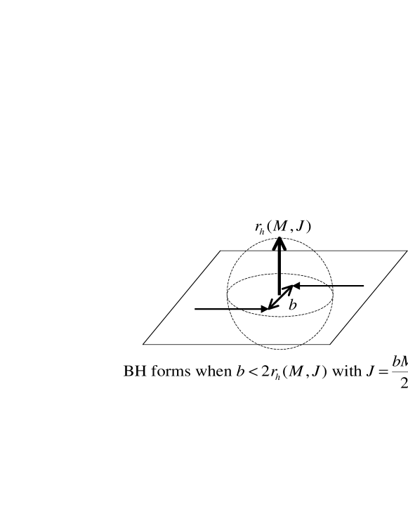
Figure 1: Schematic picture for the condition of the black hole formation.

Since $r_{h}(M,J)$ is a monotonically decreasing function of $J$ for fixed $M$, there is a maximum impact parameter $b_{\mathrm{max}}$ which saturates the inequality (2):

$$b_{\mathrm{max}}(M) =2\left[1+\left(\frac{n+2}{2}\right)^{2}\right]^{-{1\over n+1}}r_{S}(M),$$ (3)

giving the black hole production cross section $\sigma=\pi b_{\mathrm{max}}^{2}$. The formula (3) fits the numerical result of $b_{\mathrm{max}}$ with full consideration of general relativity by Yoshino and Nambu [Yoshino:2002tx] within an accuracy of less than 1.5% for $n\geq 2$ and 6.5% for $n=1$.

We note that this result is obtained in the approximation where we neglect all the effects of emissions during the formulation of the black hole (balding phase), i.e. we assume that the initial c.m. energy $M_{i}$ and angular momentum $J_{i}$ become directly the resultant black hole mass $M=M_{i}$ and angular momentum $J=J_{i}$. The coincidence of our result with the numerical study suggests that this approximation is actually viable for higher dimensional black hole formation at least unless $b$ is very close to $b_{\mathrm{max}}$.

Once we neglect the balding phase, the initial impact parameter $b$ directly leads to the resultant angular momentum of the black hole $J=bM/2$. Since the impact parameter $[b,b+db]$ contributes to the cross section $2\pi bdb$, we obtain the (differential) production cross section of the black hole with mass $M$ and angular momentum in $[J,J+dJ]$

$$d\sigma(M,J) =\begin{cases}8\pi JdJ/M^{2}&(J<J_{\mathrm{max}})\\ 0&(J>J_{\mathrm{max}})\end{cases},$$ (4)

where

$$J_{\mathrm{max}} =\frac{b_{\mathrm{max}}M}{2}=j_{n}\,\left(\frac{M}{M_{P}}\right)^{n+2\over n+1},$$ (5)

with the values of $j_{n}$ summarized in Table 2.1.

Maximum angular momentum $n$ 0 1 2 3 4 5 6 7 $j_{n}$ 0.0398 0.256 0.531 0.815 1.09 1.37 1.63 1.88 $k_{n}$ 0.0159 0.125 0.228 0.251 0.214 0.155 0.101 0.0603 $k_{n}/j_{n}$ 0.399 0.489 0.429 0.308 0.195 0.114 0.0619 0.0320 $j_{n}$ and $k_{n}$ are $J_{\mathrm{max}}$ and $J_{\mathrm{min}}$ in units of $(M/M_{P})^{n+2\over n+1}$ required for black hole and black ring formations, respectively.

The differential cross section (4) linearly increases with the angular momentum and the black hole tends to be produced with large angular momentum. For typical mass of the black hole produced at LHC $M/M_{P}\sim 5$, the value of $J_{\mathrm{max}}$ is $J_{\mathrm{max}}\sim 3,5,\ldots,10$ and 12 for $n=1,2,\ldots,6$ and 7, respectively; for large $n$, the angular momentum is not only sizable but also larger than the mass in Planck units and hence is even safer to be treated semi-classically than the mass is.

Integrating the expression (4), we obtain

$$\sigma(M) =\pi b_{\mathrm{max}}^{2}=4\left[1+\left(\frac{n+2}{2}\right)^{2}\right]^{-{2\over n+1}}\,\pi r_{S}(M)^{2}=F\,\pi r_{S}(M)^{2},$$ (6)

where the form factor $F$ is summarized in Table 2.1.

Comparison of analytical and numerical results for form factor $n$ 0 1 2 3 4 5 6 7 $F_{\mathrm{Numerical}}$ [Yoshino:2002tx] 0.647 1.084 1.341 1.515 1.642 1.741 1.819 1.883 $F_{\mathrm{Analytic}}$ 1.000 1.231 1.368 1.486 1.592 1.690 1.780 1.863 $F$ gives the form factor $F=\sigma/\pi r_{S}^{2}$.

This result implies that, apart from the four-dimensional case, we would underestimate the production cross section of black holes if we do not take the angular momentum into account.

2.2 Black rings

Black holes can have various non-trivial topologies in higher dimensions. In particular in five dimensions ($n=1$) one can construct an explicit solution for a stationary rotating black ring which is homeomorphic to $S^{1}\times S^{2}$ [Emparan:2001wn]. Here we consider the possibility of higher dimensional $S^{1}\times S^{n+1}$ black ring formation. Since we do not know how to extend the five dimensional solution to $(4+n)$ dimensions, we work in the Newtonian approximation for ring dynamics assuming that nonlinear effects will not change the qualitative features. Let us consider a rotating massive circle with radius $\ell$, mass $M$ and angular momentum $J$ in $(4+n)$-spacetime dimensions. For given $J$, the gravitational attraction $F_{g}$ and centrifugal force $F_{c}$ are

$$F_{g} \sim{GM^{2}\over\ell^{2+n}}, F_{c} \sim{J^{2}\over M\ell^{3}},$$ (7)

where $G$ is the $(4+n)$-dimensional Newton constant. Therefore we expect that the stationary solution is allowed only for $n=1$ and that the ring either shrinks or explodes monotonically for $n\geq 2$. Let $r$ be the Schwarzschild radius of the point mass in the $(3+n)$-dimensional effective theory which is obtained by integrating along the $S^{1}$ direction: $r\sim(GM/\ell)^{1/n}$. Two conditions must hold for a black ring to form in flat space picture:

1. $\ell>r$ must hold so that the hole of doughnut is not filled up;

2. $F_{c}>F_{g}$ must hold so that the ring does not start to shrink but to explode.

These conditions result in the following minimum value for the angular momentum:

$$J \mathrel{\mathchoice{\lower 3.0pt\vbox{\halign{$\m@th\displaystyle\hfill#\hfil$\cr>\crcr\sim\crcr}}}{\lower 3.0pt\vbox{\halign{$\m@th\textstyle\hfill#\hfil$\cr>\crcr\sim\crcr}}}{\lower 3.0pt\vbox{\halign{$\m@th\scriptstyle\hfill#\hfil$\cr>\crcr\sim\crcr}}}{\lower 3.0pt\vbox{\halign{$\m@th\scriptscriptstyle\hfill#\hfil$\cr>\crcr\sim\crcr}}}}J_{\mathrm{min}}=k_{n}\left(M\over M_{P}\right)^{n+2\over n+1},$$ (16)

where the values of $k_{n}$ are summarized in Table 2.1. This result shows that when $n$ is large, $J_{\mathrm{min}}$ for exploding black rings is one or two order(s) of magnitude smaller than $J_{\mathrm{max}}$ to form a virtual event horizon shown in Fig. 1 (i.e. to have strong non-perturbative gravitational interactions). Therefore we expect that the exploding black rings are possibly produced if there are many extra dimensions, though they will suffer from the black string instability when they become sufficiently large thin rings and their fate is unpredictable at this stage.

3 Evaporation

Black holes radiate mainly on the brane [Emparan:2000rs]. So we study brane field emission from a higher dimensional black hole.

3.1 Brane field equations

We make the following ansatz for the Newman-Penrose null tetrads:

$$n =dt-a\sin^{2}\vartheta d\varphi-{\Sigma\over\Delta}dr,$$

$$n^{\prime} ={\Delta\over 2\Sigma}\left(dt-a\sin^{2}\vartheta d\varphi\right)+\frac{1}{2}dr,$$

$$m ={i\sin\vartheta\over 2^{1/2}(r+ia\cos\vartheta)}\left[adt-(r^{2}+a^{2})d\varphi\right]-{r-ia\cos\vartheta\over 2^{1/2}}d\vartheta,$$

$$m^{\prime} =\bar{m},$$ (17)

where

$$\Sigma =r^{2}+a^{2}\cos^{2}\vartheta, \Delta =r^{2}+a^{2}-\mu r^{1-n}.$$ (18)

It is straightforward to check that Eq. (17) results in the correct form of the induced four dimensional metric (of the totally geodesic probe brane) in the higher dimensional Kerr field

$$g =\left(1-\frac{\mu r^{-n+1}}{\Sigma}\right)dt^{2}-\sin^{2}\vartheta\left(r^{2}+a^{2}+a^{2}\sin^{2}\vartheta\frac{\mu r^{-n+1}}{\Sigma}\right)d\varphi^{2}$$

$$\quad+2a\sin^{2}\vartheta\frac{\mu r^{-n+1}}{\Sigma}dtd\varphi-\frac{\Sigma}{\Delta}dr^{2}-\Sigma d\vartheta^{2}.$$ (19)

The parameters $\mu$ and $a$ are related to the mass $M$ and angular momentum $J$ of the higher dimensional black hole by

$$M =\frac{(n+2)A_{n+2}}{16\pi G}\mu, J =\frac{2}{n+2}Ma,$$ (20)

where $A_{n+2}=2\,\pi^{n+3\over 2}/\Gamma(\frac{n+3}{2})$ is the area of the unit sphere $S^{n+2}$.

Utilizing the null tetrads (17) one can show that the brane field equations for a massless field with spin $s=0,\frac{1}{2}$ and 1 are separable

$${1\over\sin\vartheta}{d\over d\vartheta}\left(\sin\vartheta{dS\over d\vartheta}\right)+\left[(s-a\omega\cos\vartheta)^{2}-(s\cot\vartheta+m\csc\vartheta)^{2}-s(s-1)+A\right]S=0,$$ (21)

$$\Delta^{-s}{d\over dr}\left(\Delta^{s+1}{dR\over dr}\right)$$

$$\qquad+\left[{K^{2}\over\Delta}+s\left(4i\omega r-i{\Delta_{,r}K\over\Delta}+\Delta_{,rr}-2\right)-A+2ma\omega-a^{2}\omega^{2}\right]R=0,$$ (22)

where $K=(r^{2}+a^{2})\omega-ma$, $A$ is the angular eigenvalue, and the following decomposition is employed

$$\Phi =\int d\omega\,e^{-i\omega t}\sum_{m}e^{im\varphi}\sum_{l}R_{\omega lm}(r)S_{\omega lm}(\vartheta).$$ (23)

(Here and hereafter, $m$ stands for a number in the decomposition (23) rather than the 1-form in Eq. (17).) This is one of our main results. The angular part (21) is not modified from four dimensions and can be solved in terms of the spin-weighted spheroidal harmonics ${}_{s}S_{lm}(a\omega;\vartheta,\varphi)$ with the angular eigenvalue

$$A =l(l+1)-s(s+1)-{2ms^{2}\over l(l+1)}a\omega+O\left((a\omega)^{2}\right).$$ (24)

3.2 Greybody factors

The greybody factors $\Gamma$ determine the Hawking radiation for each brane mode:

$$\frac{dN_{s,l,m}}{dt\,d\omega\,d\varphi\,d\cos\vartheta} =\frac{1}{2\pi}\frac{{}_{s}\Gamma_{l,m}(r_{h},a;\omega)}{e^{2\pi\widetilde{Q}}-(-1)^{2s}}\left|{}_{s}S_{lm}(a\omega;\vartheta,\varphi)\right|^{2},$$ (25)

where $\widetilde{Q}=(\omega-m\Omega)/2\pi T$, and hence determine the spectrum of the decay products of the black hole completely (up to a few quanta emitted in the Planck phase where the semi-classical treatment of the black hole radiation breaks down). In most literature the greybody factors are assumed to take the form of the geometrical optics (g.o.) limit:

$$\Gamma_{g.o.} =\left(\frac{n+3}{2}\right)^{2\over n+1}\frac{n+3}{n+1}(r_{h}\omega)^{2}.$$ (26)

Once we obtain the brane field equation (22), we can calculate $\Gamma$ for each mode as the absorption probability at infinity with purely ingoing boundary condition put at the horizon. We define the following dimensionless quantities

$$\xi ={r-r_{h}\over r_{h}}, \widetilde{\omega} =r_{h}\omega.$$ (27)

Then $\widetilde{Q}$ can be written as $\widetilde{Q}=(1+a_{*}^{2})\widetilde{\omega}-ma_{*}$ where $a_{*}=a/r_{h}$. In five dimensions ($n=1$), we solve the radial equation (22) both in the near-horizon and far-field limits $\xi\ll 1/\widetilde{\omega}$ and $\xi\gg 1+|\widetilde{Q}|$, respectively,

$$R_{\mathrm{NH}} =\left(\frac{\xi}{2}\right)^{-s-\frac{i\widetilde{Q}}{2}}\left(1+\frac{\xi}{2}\right)^{-s+\frac{i\widetilde{Q}}{2}}{}_{2}F_{1}(-l-s,l-s+1,1-s-i\widetilde{Q};-\frac{\xi}{2}),$$

$$R_{\mathrm{FF}} =B_{1}e^{-i\widetilde{\omega}\xi}\left(\frac{\xi}{2}\right)^{l-s}{}_{1}F_{1}(l-s+1,2l+2;2i\widetilde{\omega}\xi)$$

$$\mbox{}+B_{2}e^{-i\widetilde{\omega}\xi}\left(\frac{\xi}{2}\right)^{-l-s-1}{}_{1}F_{1}(-l-s,-2l;2i\widetilde{\omega}\xi),$$ (28)

where ${}_{2}F_{1}$ and ${}_{1}F_{1}$ are hypergeometric functions. Then we match both solutions at the consistent overlapping region $1+|\widetilde{Q}|\ll\xi\ll 1/\widetilde{\omega}$ in the low frequency limit $\omega\ll 1/r_{h}$. By this matching we obtain the constants $B_{1}$ and $B_{2}$ in terms of $s,l$ and $\widetilde{Q}$, which lead to the following analytic formula for the greybody factor:

$$\Gamma =1-\left|\frac{1-C}{1+C}\right|^{2},$$ (29)

where

$$C =\frac{(4i\widetilde{\omega})^{2l+1}}{4}\left(\frac{(l+s)!(l-s)!}{(2l)!(2l+1)!}\right)^{2}\left(-i\widetilde{Q}-l\right)_{2l+1},$$ (30)

with $(\alpha)_{n}=\prod_{n^{\prime}=1}^{n}(\alpha+n^{\prime}-1)$ being Pochhammer’s symbol. For concreteness, we write down the explicit expansion of Eq. (29) up to $O(\widetilde{\omega}^{6})$ terms

$${}_{0}\Gamma_{0,0} =4\widetilde{\omega}^{2}-8\widetilde{\omega}^{4}+O(\widetilde{\omega}^{6}),$$

$${}_{0}\Gamma_{1,m} =\frac{4\widetilde{Q}\widetilde{\omega}^{3}}{9}\left(1+\widetilde{Q}^{2}\right)+O(\widetilde{\omega}^{6}),$$

$${}_{0}\Gamma_{2,m} =\frac{16\widetilde{Q}\widetilde{\omega}^{5}}{2025}\left(1+\frac{5\widetilde{Q}^{2}}{4}+\frac{\widetilde{Q}^{4}}{4}\right)+O(\widetilde{\omega}^{10}),$$

$${}_{\frac{1}{2}}\Gamma_{\frac{1}{2},m} =\widetilde{\omega}^{2}\left(1+4\widetilde{Q}^{2}\right)-\frac{\widetilde{\omega}^{4}}{2}\left(1+4\widetilde{Q}^{2}\right)^{2}+O(\widetilde{\omega}^{6}),$$

$${}_{\frac{1}{2}}\Gamma_{\frac{3}{2},m} =\frac{\widetilde{\omega}^{4}}{36}\left(1+\frac{40\widetilde{Q}^{2}}{9}+\frac{16\widetilde{Q}^{4}}{9}\right)+O(\widetilde{\omega}^{8}),$$

$${}_{1}\Gamma_{1,m} =\frac{16\widetilde{Q}\widetilde{\omega}^{3}}{9}\left(1+\widetilde{Q}^{2}\right)+O(\widetilde{\omega}^{6}),$$

$${}_{1}\Gamma_{2,m} =\frac{4\widetilde{Q}\widetilde{\omega}^{5}}{225}\left(1+\frac{5\widetilde{Q}^{2}}{4}+\frac{\widetilde{Q}^{4}}{4}\right)+O(\widetilde{\omega}^{10}).$$ (31)

We have shown the greybody factors for the higher dimensional Kerr black hole. That of the Schwarzschild black hole is included in the limit $a_{*}\rightarrow 0$ ($\widetilde{Q}\rightarrow\widetilde{\omega}$). Note that the low frequency behavior of vector ($s=1$) is different from g.o. limit (26) in its powers of $\widetilde{\omega}$ even in the limit $a_{*}\rightarrow 0$. We can see that the numerical coefficient quickly becomes smaller as $l$ becomes larger.

3.3 Radiation from Randall-Sundrum black hole

In Figs. 2–4, we show the power spectra for spin $s=0$, $\frac{1}{2}$ and 1 fields.

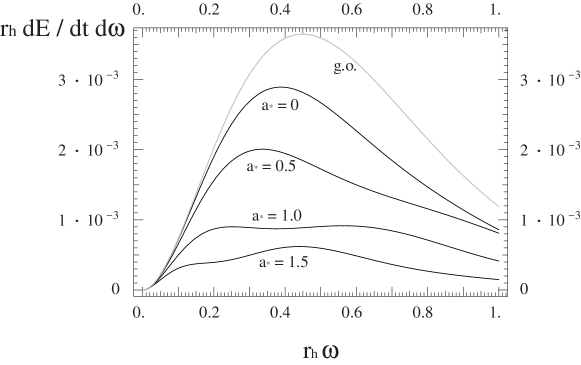
Figure 2: Scalar ($s=0$) power spectrum $r_{h}dE/dt\,d\omega$ vs $r_{h}\omega$. The gray line is the geometrical optics limit.

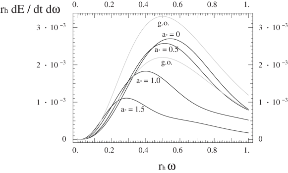
Figure 3: Spinor ($s=\frac{1}{2}$) power spectrum $r_{h}dE/dt\,d\omega$ vs $r_{h}\omega$. Upper gray line is the geometrical optics limit (lower one is multiplied by 2/3; see text).

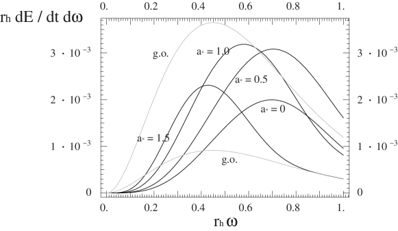
Figure 4: Vector ($s=1$) power spectrum $r_{h}dE/dt\,d\omega$ vs $r_{h}\omega$. Upper gray line is the geometrical optics limit (lower one is multiplied by 1/4; see text).

The black lines are our results from $a_{*}=0$ to 1.5. (The maximum $a_{*}$ allowed for the black hole production by Eq. (5) is $(a_{*})_{\mathrm{max}}=\frac{n+2}{2}=1.5$.) Note that our approximation is valid for $\widetilde{\omega}<\min(1,a_{*}^{-1})$. The gray line is the power spectrum in the g.o. limit (26). (For spinor and vector, the lower gray line is multiplied by the phenomenological weighting factor 2/3 and 1/4, respectively, which are introduced to mimic the four dimensional result in some papers.)

We can see that the spectrum is substantially different from the g.o. limit. (The low frequency behavior of vector emission is different from the g.o. limit in its powers of $\widetilde{\omega}$; see Fig. 5 in the log-log plot.)

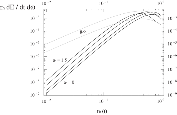
Figure 5: Vector ($s=1$) power spectrum $r_{h}dE/dt\,d\omega$ vs $r_{h}\omega$ in a log-log plot. Upper gray line is the geometrical optics limit (lower one is multiplied by 1/4; see text).

When the black hole is highly rotating (i.e. when $a_{*}$ is large), the power spectrum is substantially reduced from the g.o. limit especially for scalars and spinors ($s=0$ and $\frac{1}{2}$). This can be considered as superradiant effect enhancing the higher spin emission ($s=1$) compared to the lower ones ($s=0$ and $\frac{1}{2}$). (This can also be seen by comparing the height of the peaks in Figs. 7 and 8.) We expect that this superradiance will be more significant when $n$ is large since $(a_{*})_{\mathrm{max}}={n+2\over 2}$ is much larger for, say, $n=7$ than for $n=1$ making the higher powers of $\widetilde{Q}$ ($\simeq-ma_{*}$) more significant in Eq. (31) (or in its counterpart for $n\geq 2$).

In Figs. 6–8, we present the angular dependent power spectra for spin $s=0$, $\frac{1}{2}$ and 1 fields when $a_{*}=(a_{*})_{\mathrm{max}}=1.5$.

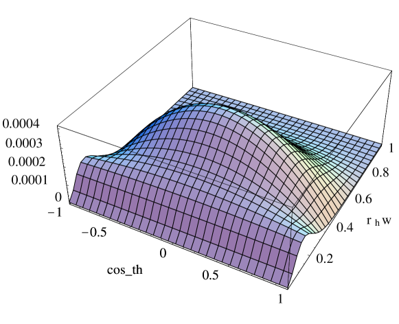
Figure 6: Scalar ($s=0$) power spectrum $r_{h}dE/dt\,d\omega\,d\cos\vartheta$ vs $r_{h}\omega$ and $\cos\vartheta$ for $a_{*}=1.5$

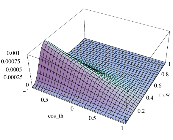
Figure 7: Spinor ($s=\frac{1}{2}$) power spectrum $r_{h}dE/dt\,d\omega\,d\cos\vartheta$ vs $r_{h}\omega$ and $\cos\vartheta$ for $a_{*}=1.5$

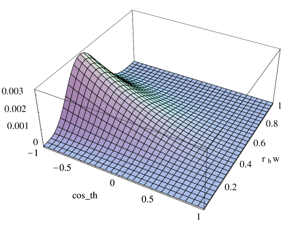
Figure 8: Vector ($s=1$) power spectrum $r_{h}dE/dt\,d\omega\,d\cos\vartheta$ vs $r_{h}\omega$ and $\cos\vartheta$ for $a_{*}=1.5$

Recall that our approximation is valid for $\widetilde{\omega}<\min(1,a_{*}^{-1})$. We observe that there is a large angular dependence. Note that $\cos\vartheta=1$ ($-1$) is the direction (anti)parallel to the angular momentum of the black hole which is perpendicular to the beam axis and that $\cos\vartheta=0$ contains the direction of beam axis (for some value of $\varphi$). (Even after averaging over the rotation around the beam axis, there still remains strong angular dependences for spinor and vector fields.) We note that since only one helicity component is used in Figs. 7 and 8, the large up-down asymmetry does not imply a parity violation when we sum up the opposite components. (Neutrinos are exceptional since they do not have opposite helicity states to be paired with them.) The angular dependence shown in Figs. 6–8 vanishes when we take the limit $a_{*}\rightarrow 0$.

4 Summary and discussion

We have shown that black holes tend to be produced with large angular momentum and that the production cross section of the black hole increases when one takes this into account. We have also estimated the possibility of black ring formation and found that it may be produced when there are many extra dimensions, though its fate is currently unknown. It would be interesting to estimate the black ring production cross section too. (One way might be to follow our argument for the black hole production.)

We have presented the spin $s=0$, $\frac{1}{2}$ and 1 brane field equations for the $(4+n)$-dimensional Kerr black hole and have shown that they are separable. We have analytically solved them for the five dimensional case ($n=1$) and obtained the greybody factor in the low frequency limit. Note that our results include the case of Schwarzschild black hole in the limit $a\rightarrow 0$. This is the first time that the greybody factors of brane spinor and vector fields are obtained for the higher dimensional black hole regardless of whether it is rotating or not. We have found that the resulting power spectra are substantially modified from the geometrical optics limit and that there is strong angular dependence. We expect that these features remain qualitatively the same for any number of extra dimensions $n$.

It is important to obtain the greybody factors for higher dimensional Kerr black hole numerically without relying on the low frequency expansion to determine the total radiation of the black hole from its birth till the end for general $n$. This work is in progress.

Appendix A Brane field equations

In Ref. [Kanti:2002ge] which appeared after our work, the brane field equation for the higher dimensional Schwarzschild black hole (i.e. the limit $a\rightarrow 0$ in our language),

$$\Delta^{s}{d\over dr}\left[\Delta^{1-s}{dR_{s}\over dr}\right]+\Biggl{\{}{\Sigma^{2}\omega^{2}-is\omega\Sigma\partial_{r}\Delta\over\Delta}+2is\omega\partial_{r}\Sigma-\Lambda\Biggr{.}$$

$$\qquad\left.+\Delta\left(s-\frac{1}{2}\right)\left[\partial_{r}\left(\partial_{r}\Sigma\over\Sigma\right)+\left(s-\frac{1}{2}\right)\left(\partial_{r}\Sigma\over\Sigma\right)^{2}+(1-s){\partial_{r}\Sigma\over\Sigma}{\partial_{r}\Delta\over\Delta}\right]\right\}R_{s}=0,$$ (A.32)

with $\Lambda=j(j+1)-s(s-1)$ being the angular eigenvalue and $\Sigma=r^{2}$, is derived from the Cvetic-Larsen equation which essentially relies on the fact that $\Delta_{,rr}-2$ vanishes in four dimensions ($n=0$), though not in higher dimensions ($n\geq 1$).

From Eq. (22) we can redefine the radial function as $R=\Delta^{s}R_{KM}$ to obtain

$$\Delta^{s}{d\over dr}\left[\Delta^{1-s}{dR_{KM}\over dr}\right]$$

$$\qquad+\left[{K^{2}-isK\Delta_{,r}\over\Delta}+4isr\omega-2s-A+2ma\omega-(a\omega)^{2}\right]R_{KM}=0.$$ (A.33)

In the limit $a\rightarrow 0$, $K$ and the angular eigenvalue $A$ behave as

$$K \rightarrow r^{2}\omega=\Sigma\omega, A \rightarrow l(l+1)-s(s+1)=\Lambda-2s,$$ (A.34)

and therefore Eq. (A.32) becomes identical to Eq. (A.33) when one deletes the second line of Eq. (A.32):

$$\Delta\left(s-\frac{1}{2}\right)\left[\partial_{r}\left(\partial_{r}\Sigma\over\Sigma\right)+\left(s-\frac{1}{2}\right)\left(\partial_{r}\Sigma\over\Sigma\right)^{2}+(1-s){\partial_{r}\Sigma\over\Sigma}{\partial_{r}\Delta\over\Delta}\right] \longrightarrow 0.$$ (A.35)

(The l.h.s. of Eq. (A.35) becomes zero for $s=\frac{1}{2}$ and 1, though not for $s=0$, and hence the result of Ref. [Kanti:2002ge] studying the former cases remains unchanged after this correction.) This check is first presented in Ref. [Harris:2003eg] by utilizing our Newman-Penrose tetrads (17) and by rederiving the the master equation (22) both in the limit $a\rightarrow 0$.

References

- [1] N. Arkani-Hamed, S. Dimopoulos, and G. R. Dvali, “The hierarchy problem and new dimensions at a millimeter,” Phys. Lett. B429 (1998) 263–272, hep-ph/9803315.
- [2] L. Randall and R. Sundrum, “A large mass hierarchy from a small extra dimension,” Phys. Rev. Lett. 83 (1999) 3370–3373, hep-ph/9905221.
- [3] S. B. Giddings and S. Thomas, “High energy colliders as black hole factories: The end of short distance physics,” Phys. Rev. D65 (2002) 056010, hep-ph/0106219.
- [4] S. Dimopoulos and G. Landsberg, “Black holes at the LHC,” Phys. Rev. Lett. 87 (2001) 161602, hep-ph/0106295.
- [5] H. Yoshino and Y. Nambu, “Black hole formation in the grazing collision of high- energy particles,” Phys. Rev. D67 (2003) 024009, gr-qc/0209003.
- [6] T. Banks and W. Fischler, “A model for high energy scattering in quantum gravity,” hep-th/9906038.
- [7] R. Sundrum, “Fat Euclidean gravity with small cosmological constant,” hep-th/0310251.
- [8] S. Dimopoulos and R. Emparan, “String balls at the LHC and beyond,” Phys. Lett. B526 (2002) 393–398, hep-ph/0108060.
- [9] G. T. Horowitz and J. Polchinski, “A correspondence principle for black holes and strings,” Phys. Rev. D55 (1997) 6189–6197, hep-th/9612146.
- [10] D. Ida, K.-y. Oda, and S. C. Park, “Rotating black holes at future colliders: Greybody factors for brane fields,” Phys. Rev. D67 (2003) 064025, hep-th/0212108.
- [11] L. A. Anchordoqui, J. L. Feng, H. Goldberg, and A. D. Shapere, “Updated limits on TeV-scale gravity from absence of neutrino cosmic ray showers mediated by black holes,” hep-ph/0307228.
- [12] R. Emparan and H. S. Reall, “A rotating black ring in five dimensions,” Phys. Rev. Lett. 88 (2002) 101101, hep-th/0110260.
- [13] R. Emparan, G. T. Horowitz, and R. C. Myers, “Black holes radiate mainly on the brane,” Phys. Rev. Lett. 85 (2000) 499–502, hep-th/0003118.
- [14] P. Kanti and J. March-Russell, “Calculable corrections to brane black hole decay. II: Greybody factors for spin 1/2 and 1,” Phys. Rev. D67 (2003) 104019, hep-ph/0212199.
- [15] C. M. Harris and P. Kanti, “Hawking radiation from a (4+n)-dimensional black hole: Exact results for the Schwarzschild phase,” JHEP 10 (2003) 014, hep-ph/0309054.