Abstract

A review on the requirements of chiral symmetry on effective quark models is presented. The connection between the pion Salpeter amplitude and the mass gap equation is discussed. Hadronic scattering, notably, $\pi\;\pi$ scattering is presented. The constraints imposed by chiral symmetry between difractive quark scattering and quark-quark annihilation is presented. Hadronic coupled channels as a consequence of quark-quark annihilation are discussed together with the ${}^{3}P_{0}$ mecahnism. Graphical-rules diagrams are intoduced as a means to evaluate hadronic coupled channel transition potentials. Their role in finding transition potentials responsible, in the scalar sector, for low energy resonances, predicted long ago, and found recently, is also discussed

1 Introduction

In 2+1 dimensions, the Hamiltonian of a relativistic fermion in an external field $A_{\mu}$ has the following form :

$$H=\int d^{2}x\ \bar{\psi}(x)\left[-i\gamma^{j}D_{j}+m\right]\psi(x)\ ,$$ (1)

with $D_{\mu}=\partial_{\mu}+ieA_{\mu}\ (\mu=0,1,2)$.

In 2+1 dimensions there are two inequivalent representations of the Dirac algebra, described by the matrices

$$\tilde{\gamma}^{0}=\sigma_{3}\ ,\ \tilde{\gamma}^{1}=i\sigma_{1}\ ,\ \tilde{\gamma}^{2}=i\sigma_{2}\ ,\$$

$$\tilde{\gamma}^{0}=-\sigma_{3}\ ,\ \tilde{\gamma}^{1}=-i\sigma_{1}\ ,\ \tilde{\gamma}^{2}=-i\sigma_{2}.$$ (2)

The theory is invariant under an $U(2)$ symmetry, which breaks down to $U(1)\times U(1)$ for $m\neq 0.$

It is convenient to choose the Landau gauge $A_{\mu}=-By\ \delta_{\mu 1}$, where $B>0$ is the magnetic field strength. The problem is solvable and the solution in the chiral version has the structure

$$\psi^{B}(\bf{x},t)=\left(\begin{array}[c]{c}\psi_{1}^{B}\\ \psi_{2}^{B}\end{array}\right),$$ (3)

where $\psi_{1,2}^{B}(x)$ are the spinors associated to the two inequivalent representations of the Dirac algebra.

2 An example of Valatin-Bogolioubov Transformations

We need three steps to construct, from the wave-function of a free particle, the wave-function of a particle in a magnetic field. Here I present a generalization of the method of ref. [1] done with G. Marques and R. Felipe.

2.1 Step1:Valatin-Bogolioubov rotations

From,

$$\psi(\bf{x})=\sum\limits_{\bf{p}}\frac{1}{\sqrt{L_{x}L_{y}}}\left\{u(\bf{p})\ a_{\bf{p}}+v(\bf{p})\ b_{-\bf{p}}^{\dagger}\right\}e^{i\bf{p}\cdot\bf{x}}$$ (4)

with,

$$u(\bf{p})=\sqrt{\frac{E_{\bf{p}}+m}{2E_{\bf{p}}}}\left[\begin{array}[]{c}1\\ \frac{p_{y}-ip_{x}}{{E_{\bf{p}}+m}}\end{array}\right];v(\bf{p})=\sqrt{\frac{E_{\bf{p}}+m}{2E_{\bf{p}}}}\left[\begin{array}[]{c}-\frac{p_{y}+ip_{x}}{{E_{\bf{p}}+m}}\\ 1\end{array}\right]$$ (9)

$$\left\{a^{\dagger}_{\bf{p}},a_{\bf{p}^{\prime}}\right\}=\left\{b^{\dagger}_{\bf{p}},\;b_{\bf{p}^{\prime}}\right\}=\delta_{p_{x}p^{\prime}_{x}}\delta_{p_{y}p^{\prime}_{y}},\;\;E_{\bf{p}}=\sqrt{m^{2}+|\bf{p}|^{2}}.$$ (10)

The $u$ and $v$ spinors are the solutions of the Dirac equation for positive and negative energy respectively.

Step 1: preform a canonical transformation given by,

$$\left[\begin{array}[]{c}\tilde{a}_{\bf{p}}\\ \tilde{b}^{\dagger}_{-\bf{p}}\end{array}\right]=R_{\phi}(\bf{p})\left[\begin{array}[]{c}a_{\bf{p}}\\ b^{\dagger}_{-\bf{p}}\end{array}\right]\hskip 14.22636pt\left[\begin{array}[]{c}\tilde{u}\\ \tilde{v}\end{array}\right]=R_{\phi}^{*}(\bf{p})\left[\begin{array}[]{c}u(\bf{p})\\ v(\bf{p})\end{array}\right]$$ (11)

with,

$$R_{\phi}(\bf{p})=\left[\begin{array}[]{cc}\cos\phi&-\sin\phi\ (\hat{p}_{y}+i\hat{p}_{x})\\ \sin\phi\ (\hat{p}_{y}-i\hat{p}_{x})&\cos\phi\end{array}\right],$$ (12)

and,

$$\hat{p}=\frac{\bf p}{|p|},\;\cos\phi=\sqrt{\frac{E_{\bf{p}}+m}{2E_{\bf{p}}}},\;\sin\phi=\sqrt{\frac{E_{\bf{p}}-m}{2E_{\bf{p}}}}.$$ (13)

The vacuum associated to the new operators $\tilde{a}$ and $\tilde{b}$ is given by

$$|\tilde{0}\rangle=S|0\rangle=\prod_{\bf{p}}(\cos\phi+\sin\phi\,a^{\dagger}_{\bf{p}}b^{\dagger}_{-\bf{p}})|0\rangle\$$ (14)

with, $\tilde{a}_{\bf{p}}|\tilde{0}\rangle=0,\;\tilde{b}_{\bf{p}}|\tilde{0}\rangle=0$.

Think of $\psi(\bf{x})=\sum\limits_{\bf{p}}\frac{1}{\sqrt{L_{x}L_{y}}}\left\{u(\bf{p})\ a_{\bf{p}}+v(\bf{p})\ b_{-\bf{p}}^{\dagger}\right\}e^{i\bf{p}\cdot\bf{x}}$ as an inner product between the Hilbert space spanned by the spinors $\{u,v\}$ and the Fock space generated by $\{a,b\}$. This inner product is invariant under V-B transformations: any rotation in the Fock space must engender a counter-rotation in the Hilbert space.

The choice of $\phi$ was arranged to ensure the new spinors $\tilde{u}$ and $\tilde{v}$ to be momentum independent:

$$\tilde{u}=\left[\begin{array}[]{c}0\\ 1\end{array}\right],\;\;\tilde{v}=\left[\begin{array}[]{c}1\\ 0\end{array}\right]$$ (15)

so that all the momentum dependence of $\psi$ is stored in $\{\tilde{a}_{\bf{p}},\tilde{b}_{\bf{p}}\}=S\{\hat{a},\hat{b}\}S$.

2.2 Step II: Landau Levels

Step II: Use the Landau Level representation.

Use,

$$e^{ip_{y}y}=e^{-i\ell^{2}p_{x}p_{y}}\sqrt{2\pi}\sum_{n=0}^{\infty}\,i^{n}\omega_{n}(\xi)\,\omega_{n}(\ell p_{y})$$

$$\omega_{n}(x)=(2^{n}n!\sqrt{\pi})^{-1/2}e^{-x^{2}/2}H_{n}(x)\;l=\sqrt{|eB|},\;\;\xi=\frac{y}{l}+lp_{x}.$$ (16)

The wave function in the new basis can be written in the following way:

$$\psi(\bf{x})=\sum\limits_{n\,p_{x}}\frac{1}{\sqrt{\ell L_{x}}}\left\{\hat{u}_{np_{x}}(y)\ \hat{a}_{np_{x}}+\hat{v}_{np_{x}}(y)\ \hat{b}_{n-p_{x}}^{\dagger}\right\}e^{ip_{x}x}$$

$$\left[\begin{array}[]{c}\hat{a}_{np_{x}}\\ \hat{b}^{\dagger}_{n-p_{x}}\end{array}\right]=\sum_{p_{y}}\frac{i^{n}\sqrt{2\pi\ell}}{\sqrt{L_{y}}}\left[\begin{array}[]{cc}\omega_{n}(\ell p_{y})&0\\ 0&-\omega_{n-1}(\ell p_{y})\end{array}\right]\left[\begin{array}[]{c}\tilde{a}_{\bf{p}}\\ \tilde{b}^{\dagger}_{-\bf{p}}\end{array}\right]$$ (23)

with,

$$\left[\begin{array}[]{c}\hat{u}_{np_{x}}(y)\\ \hat{v}_{np_{x}}(y)\end{array}\right]=\left[\begin{array}[]{cc}\omega_{n}(\xi)&0\\ 0&i\omega_{n-1}(\xi)\end{array}\right]\left[\begin{array}[]{c}\tilde{u}\\ \tilde{v}\end{array}\right].$$ (24)

The new operators satisfy the canonical anticommutation relations: $\left\{a^{\dagger}_{np_{x}},a_{n^{\prime}p^{\prime}_{x}}\right\}=\left\{b^{\dagger}_{np_{x}},b_{n^{\prime}p^{\prime}_{x}}\right\}=\delta_{nn^{\prime}}\ \delta_{p_{x}p^{\prime}_{x}}$. The vacuum is invariant under this change of basis, i.e., $\hat{a}_{np_{x}}|\tilde{0}\rangle=0,\;\hat{b}_{np_{x}}|\tilde{0}\rangle=0$.

There are several approaches one can adopt to obtain the mass gap equation:

• 1. It can be derived as the condition for the vacuum energy to be a minimum or,

• 2. geting rid of anomalous Bogolioubov terms or,

• 3. in the form of a Dyson equation for the fermion propagator or,

• 4. as a Ward identity.

Here we use 2.

2.3 Step 3:Mass gap equation for Landau levels

Step III: Perform yet another V.B. transformation:

$$R_{\theta_{n}}=\left[\begin{array}[]{cc}\cos\theta_{n}&-\sin\theta_{n}\\ \sin\theta_{n}&\cos\theta_{n}\end{array}\right].$$ (25)

The $\theta_{n}$ angles are to be found by imposing the vanishing of the anomalous terms in the Hamiltonian. A simple algebraic computation yields the following mass gap equations,

$$\left\{\begin{array}[]{l}(\ell\,m\cos\theta_{0}+\sin\theta_{2}/\sqrt{2})\sin\theta_{0}=0\ ,\quad n=0\ ,\\ \ell\,m\sin 2\theta_{n}-\sqrt{2n}\cos 2\theta_{n}=0\ ,\quad n>0\ ,\end{array}\right..$$ (26)

For any $n$ have the following solution: $\tan 2\theta_{n}=\sqrt{2n|eB|}/m$. The elements of the rotation matrix are given by, $\cos\theta_{n}=\sqrt{(E_{n}+m)/(2E_{n})},\;\sin\theta_{n}=\sqrt{(E_{n}-m)/(2E_{n})}$ with $E_{n}=\sqrt{m^{2}+2n|eB|}$.

It remains to construct the vacuum state in a magnetic field $|0\rangle_{B}$, annihilated by the operators $a_{np_{x}}$ and $b_{np_{x}}$ : $a_{np_{x}}|0\rangle_{B}=0\quad,\quad b_{np_{x}}|0\rangle_{B}=0$. We have,

$$|0\rangle_{B}=\prod_{n\,p_{x}}(\cos\theta_{n}+\sin\theta_{n}\,\hat{a}^{\dagger}_{np_{x}}\hat{b}^{\dagger}_{n-p_{x}})|\tilde{0}\rangle$$ (27)

Next let us consider the problem of dynamical symmetry breaking in the presence of the magnetic field. We obtain ${{}_{B}}\langle 0|\psi^{\dagger}(\bf{x})\psi(\bf{x})|0\rangle_{B}=-|eB|/(2\pi)$.

The spontaneous breaking of the $U(2)$ flavour symmetry occurs even in the absence of any additional interaction between fermions. This is an inherent property of the 2+1 dimensional Dirac theory in an external magnetic field. In 3+1 dimensions the spontaneous breakdown in a magnetic field can take place only when an “effective” mass term ($m\neq 0$) is generated. In 3+1 Dimensions these very same 3-steps can be performed. Vacuum condensates only if $m_{q}\neq 0$. For literature on this subject see [2].

3 A general class of Hamiltonians

For this talk let us consider the simplest Hamiltonian containing the ladder-Dyson-Schwinger machinery for chiral symmetry. In any case most of the results presented here do not depend on the kernel choice

$$H=\int d^{3}x\,q^{+}(x)\left(-i\overrightarrow{\alpha.}\overrightarrow{\;\nabla}\right)q(x)+\int\frac{d^{3}x\;d^{3}y}{2}J_{\mu}^{a}(x)K_{\mu\nu}^{ab}(x-y)J_{\nu}^{b}(y)$$ (28)

With, $J_{\mu}^{a}(x)=\overline{q}(x)\gamma_{\mu}\frac{\lambda^{a}}{2}q(x)$ and $K_{\mu\nu}^{ab}(x-y)=\delta^{ab}K_{\mu\nu}(|\overrightarrow{x}-\overrightarrow{y}|)$

This class of Hamiltonians has a rich structure enabling the study of a variety of hadronic phenomena controlled by global symmetries. It is Chiral compliant: The fermions know about the kernel. It reproduces in a non-trivial manner the low energy properties of pion physics like, for instance, $\pi-\pi$ scattering. And it possesses the mechanism of pole-doubling in what concerns scalar decays.

3.1 Bogolioubov Transformations

We can rotate the creation and annihilation Fock space operators as,

$$|\widetilde{0}>=Exp\left\{\widehat{Q}_{0}^{+}-\widehat{Q}_{0}\right\}|0>$$ (29)

with,

$$\widehat{Q}_{0}^{+}(\Phi)=\sum_{cf}\int d^{3}p\,\Phi(p)\,\widehat{b}_{fcs}^{+}(\overrightarrow{p})\,\widehat{d}_{fcs^{{}^{\prime}}}^{+}(-\overrightarrow{p}).$$ (30)

The matrix $M_{ss^{{}^{\prime}}}(\theta,\phi)$ carries the ${}^{3}P_{0}$ Coupling (Parity +):

$$M_{ss^{{}^{\prime}}}(\theta,\phi)=-\sqrt{8\pi}\sum_{m_{l}m_{s}}\left[\begin{array}[]{ccc}1&1&|0\\ m_{l}&m_{s}&|0\end{array}\right]\times\left[\begin{array}[]{ccc}1/2&1/2&|1\\ s&s^{{}^{\prime}}&|m_{s}\end{array}\right]y_{1m_{l}}(\theta,\phi).$$ (31)

The functions $\Phi(p)$ classify the set of infinite possible Fock spaces. The Fock space operators transform like, $\widetilde{\widehat{b}}_{cfs}(\overrightarrow{p})=S\,\widehat{b}_{cfs}\,S^{-1}$, so that,

$$\left[\begin{array}[]{l}\widetilde{\widehat{b}}\\ \widetilde{\widehat{d}}^{+}\end{array}\right]_{s}=\left[\begin{array}[]{ll}\cos\phi&-\sin\phi M_{ss^{{}^{\prime}}}\\ \sin\phi M_{ss^{{}^{\prime}}}^{\star}&\cos\phi\end{array}\right]\left[\begin{array}[]{l}\widehat{b}\\ \widehat{d}^{+}\end{array}\right]_{s^{{}^{\prime}}}.$$ (32)

We can again consider the fermion field $\Psi_{fc}(\overrightarrow{x})$ as an inner product between the Hilbert space spanned by the spinors {u,v} and the Fock space spaned by the operators {$\widehat{b}$,$\widehat{d}$}:

$$\Psi_{fc}(\overrightarrow{x})=\int d^{3}p\left[u_{s}(p)~{}b_{cfs}(\overrightarrow{p})+u_{s}(p)~{}d_{cfs}^{+}(\overrightarrow{-p})\right]e^{i\overrightarrow{p}.\overrightarrow{x}}.$$

So that requiring invariance of $\Psi_{fc}(\overrightarrow{x})$under the Fock space rotations, is tantamount to require a counter-rotation of the spinors u and v,

$$\left[\begin{array}[]{l}u\\ v\end{array}\right]=\left[\begin{array}[]{ll}\cos\phi&-\sin\phi M_{ss^{{}^{\prime}}}^{\ast}\\ \sin\phi M_{ss^{{}^{\prime}}}&\cos\phi\end{array}\right]\left[\begin{array}[]{l}u\\ v\end{array}\right].$$ (33)

The {u,v}, contain now the information on the angle $\phi(p)$ [3].

3.2 Chiral Symmetry

Consider the transformation $\Psi\rightarrow\exp\left\{-i\alpha^{a}\frac{T^{a}}{2}\gamma_{5}\right\}.$ Then,

$$H\left[m_{q}\right]\rightarrow H[m_{q}\cos\left(\frac{\alpha^{2}}{2}\right)-m_{q}\sin\left(\frac{\alpha^{2}}{2}\right)i\gamma_{5}].$$

H is chirally symmetric iff $m_{q}=0.$

Assume that $\phi$ exists and construct,

$$Q_{5}^{a}=\int d^{3}x\,\overline{\Psi}\gamma_{0}\gamma_{5}\Psi.$$ (34)

We obtain,

$$\int d^{3}x\cos\left(2\phi\right)\left[\overrightarrow{p}.\overrightarrow{\sigma}\,\widehat{b}^{+}(p)\widehat{b}(p)+(\widehat{d}^{+}\widehat{d})\right]+\sin\left(2\phi\right)\left[\underbrace{\mu_{ss^{{}^{\prime}}}\widehat{b}^{+}(p)\widehat{d}^{+}(-p)+(\widehat{d}\widehat{b})}\right].$$ (35)

It is true that for an arbitrary $\phi,\,Q_{5}^{a}|0>\neq 0,$ and because [$Q_{5}^{a},H\left(m_{q}=0\right)$]=0, we have that $Q_{5}^{a}$ acting in the vacuum creates a state, which will turn out to be the pion ($\mu_{ss^{{}^{\prime}}}$ is the spin wave function for S=0, made out of two spin 1/2’s). This state is degenerate with the vacuum.

3.3 Mass gap Equation

The Hamiltonian can be decomposed as,

$$\widehat{H}=\widehat{H}_{normal}[\phi]+\widehat{H}_{anomalous}[\phi]$$

$$\widehat{H}_{2}\left[normal\right]=\int d^{3}p\,E(p)\left[\widehat{b}_{fsc}^{+}(\overrightarrow{p})\widehat{b}_{fsc}(\overrightarrow{p})+\widehat{d}_{fsc}^{+}(-\overrightarrow{p})\widehat{d}_{fsc}(\overrightarrow{-p})\right]$$

$$\widehat{H}_{2}[anomalous]=\int d^{3}p\left[A[K]\sin(\varphi)-B[k]\cos(\varphi)\right]$$

$$\quad\quad\quad\quad\quad\quad\quad\quad\quad\times\left[M_{ss^{{}^{\prime}}}\widehat{b}_{fsc}^{+}(\overrightarrow{p})\widehat{d}_{fsc}^{+}(\overrightarrow{-p})+h.c.\right].$$ (36)

In general $\widehat{H}|0>=\widehat{H}_{anomalous}[\phi]|0>\neq 0.$

Problem: find $\phi_{0}$ such that $\widehat{H}_{anomalous}[\phi_{0}]|0>=0.$ This is the mass gap equation. Therefore we must find $\phi_{0}$ such that,

$$\left[A[K]\sin(\varphi)-B[k]\cos(\varphi)\right]=0$$ (37)

We cannot simultaneously get rid of both the anomalous terms for $\widehat{H}$ and $\widehat{Q_{5}^{a}}$. $\widehat{Q_{5}^{a}}$ will remain anomalous:

$$\widehat{Q_{5}^{a}}|0>=|\pi>.$$ (38)

Then, $\left[H,Q_{5}\right]=0$ implies that $\pi$ is massless.

We have several ways of arriving at the mass gap equation $\widehat{H}_{2}[anomalous]=0$. Let us consider two different ways (albeit related) of obtaining the Mass gap Equation,

• Minimization of $H_{0}:\frac{\delta H_{0}}{\delta\varphi}=0.$

• Ward identities.

Variation in $\phi$ is the same as to cut the fermion propagators $S_{\phi}$, so as to obtain the mass gap equation as the condition for the bilinear anomalous term of the Hamitonian to be zero–see Table 1. Another way to find the mass gap equation is to use the vectorial Ward identities [4].

TABLE 1.  : Minimization of the vacuum energy is tantamount to write the mass gap equation as the condition for the bilinear anomalous term of the Hamitonian to be zero. The mass gap equation as a Dyson series for the fermion propagator is also depicted. This series can also be obtained using the Ward identity for the vectorial current-see Eq.(3.3)

$$(p-p^{{}^{\prime}})^{\mu}\;\Gamma_{\mu}(p,p^{{}^{\prime}})=(p-p^{{}^{\prime}})^{\mu}\;\gamma_{\mu}+$$

$$\quad+i\int\frac{d^{4}q}{(2\pi)^{4}}K(q)\Omega\,S(p^{{}^{\prime}}+q)\Gamma_{\mu}(p^{{}^{\prime}}+q,p+q)\Omega S(p^{{}^{\prime}}+q)i(p-p^{{}^{\prime}})^{\mu}\,\Gamma_{\mu}(p,p^{{}^{\prime}})$$

$$\hskip 28.45274pt=S^{-1}(p^{{}^{\prime}})-S^{-1}(p)$$ (39)

Once the mass gap is solved we can go back to the Hamiltonian of Eq.(28) and identify several effective quark vertices-see fig. 1.

$$u_{s}^{\dagger}(p)\cdot\Gamma\cdot u_{s^{\prime}}(p^{\prime})\;(\;quark\;scattering\;)$$

$$v_{s}(-p)\cdot\Gamma\cdot v_{s^{\prime}}^{\dagger}(-p^{\prime})\;(\;antiquark\;scattering\;)$$

$$u_{s}^{\dagger}(p)\cdot\Gamma\cdot v_{s}(-p^{\prime})\;(\;quark-antiquark\;creation\;)$$

$$v_{s}^{\dagger}(-p)\cdot\Gamma\cdot u_{s}(p^{\prime})\;(\;quark-antiquark\;annihilation\;)$$ (40)

where the spinors u and v carry now the information on the chiral angle $\phi(p)$ [3].

Figure 1.  : The basic quark quark interactions we can extract from the Hamiltonian of Eq. (28) when dealing with one meson. We have four types of microscopic vertices. The first rightmost diagram is built with vertices $u_{s}^{\dagger}(p)\cdot\Gamma\cdot u_{s^{\prime}}(p^{\prime})$, (quark scattering) $v_{s}(-p)\cdot\Gamma\cdot v_{s^{\prime}}^{\dagger}(-p^{\prime})$, (antiquark scattering) and the remaining diagrams contain at least one vertex of either $u_{s}^{\dagger}(p)\cdot\Gamma\cdot v_{s}(p^{\prime})$, (quark-antiquark creation) or $v_{s}^{\dagger}(-p)\cdot\Gamma\cdot u_{s}(p^{\prime})$ (quark-antiquark annihilation)

Figure 2.  : Salpeter equation for mesons. Notice that the application of the microscopic quark interactions of fig. 1-a already yields two coupled channel equations. Further insertions of the microscopic interactions of fig.1-b,c,d will produce extra couplings of the meson state with two meson intermediate channels.

3.4 Pion Salpeter Amplitude

From the renormalized propagator we can construct the Bethe-Salpeter equation for mesonic states-see fig.2. We can proceed via two identical formalisms: either work

• in the Dirac Space or,

• work in the Spin Representation

To go from the Dirac representation to the spin representation it is sufficient to to construct the spin wave functions as it is exemplified in Eq. (41)

$$\chi_{\alpha\beta}^{++}(k)=u_{s1;\alpha}(k)\Phi_{s1s2}(k)\overline{v}_{s2;\beta}(-k).$$ (41)

We get,

$$\left[\begin{array}[]{ll}H^{++}&H^{+-}\\ H^{-+}&H^{--}\end{array}\right]\left[\begin{array}[]{l}\Phi^{+}\\ \Phi^{-}\end{array}\right]=m_{\pi}\,\sigma_{3}\left[\begin{array}[]{l}\Phi^{+}\\ \Phi^{-}\end{array}\right]$$ (42)

with,

$$\Phi^{+}\Longleftrightarrow\Phi^{-},\quad m_{\pi}\Longleftrightarrow-m_{\pi}.\hskip 14.22636pt(m_{\pi}=0,\;\Phi^{+}=\Phi^{-}.)$$

$$\int d^{3}k\left(\Phi^{+^{2}}-\Phi^{-^{2}}\right)=N^{-1}$$ (43)

Therefore in the space of pions we can write, not only the Hamiltonian of Eq. (28), but any Hamiltonian possessing instantaneous quark kernels, as

$$H=\sigma_{3}\left[\begin{array}[]{l}\Phi^{+}\\ \Phi^{-}\end{array}\right]m_{\pi}\left[\begin{array}[]{ll}\Phi^{+},&\Phi^{-}\end{array}\right]\sigma_{3}+\sigma_{3}\left[\begin{array}[]{l}\Phi^{-}\\ \Phi^{+}\end{array}\right]m_{\pi}\left[\begin{array}[]{ll}\Phi^{-},&\Phi^{+}\end{array}\right]\sigma_{3}.$$ (44)

4 $\pi\;\pi$ Scattering

The next logical step in the study of pion physics consists in considering $\pi\;\pi$ scattering. In the figure below we give two such examples of diagrams together with their respective mapping into pion Salpeter equations.

In the figure we also show the mapping which is always possible between a $\pi\;\pi\rightarrow\pi\;\pi$ diagram and its equivalent pion Salpeter diagram . Below we translate the above diagrams into Resonating Group Method (RGM) [5] diagrams in order to have a clearer physical picture. We have,

In the left diagrams the + sign means (gets translated) to quark propagator whereas the - sign corresponds to an antiquark propagator. Of course these $\pm$ signs correspond to the Feynman projection operators. Finally it is known [7] that the RGM evaluation of the S matrix, having Salpeter asymptotic states, is equivalent to sum all the ladder diagrams pertaining to this process. This mapping is exemplified in Eq. (45).

$$\left[\begin{array}[]{ll}\Phi^{-^{2}}&\Phi^{+^{2}}\end{array}\right]{\color[rgb]{1,0,0}\left[\begin{array}[]{ll}H^{++}&H^{+-}\\ H^{-+}&H^{--}\end{array}\right]}\left[\begin{array}[]{l}\Phi^{+^{2}}\\ \Phi^{-^{2}}\end{array}\right]\rightarrow\,{\color[rgb]{1,0,0}m_{\pi}}\left[\begin{array}[]{ll}\Phi^{-^{2}}&\Phi^{+^{2}}\end{array}\right]{\color[rgb]{1,0,0}\sigma_{3}}\left[\begin{array}[]{l}\Phi^{+}\\ \Phi^{-}\end{array}\right].$$ (45)

Using $\{\Phi^{\pm}=\sin\varphi/a\pm a\Delta,\;a=\sqrt{\frac{2}{3}}f_{\pi}m_{\pi}\}$ we obtain the Weinberg results in the point-like limit:$\sin\varphi\rightarrow 1.,\;\left\{-7/2\,m_{\pi}^{2}/f_{\pi}^{2},\quad m_{\pi}^{2}/f_{\pi}^{2}\right\}$–see ref [8] for details. It is important to stress that in no time we have made use of a particular form for the microscopic quark kernel which means that the Weinberg result is completely controlled by chiral symmetry and independent of the chiral model used.

5 The rho Resonance

As we have seen in the previous section,for a give hadronic reaction we are faced with the task of calculating both diffractive and annihilation diagrams. The next step consists in introducing coupled hadronic channels. A classical playground to study the role of quark-antiquark annihilation (creation) diagrams in the production of coupled hadronic channels is provided by the $\rho$ resonance. In the figure below we depict the skeleton diagrams contributing to the $\rho$ decay into two mesons. Notice that that the quark annihilation (creation) vertices are completely specified by the Hamiltonian of Eq. (28) and therefore will only depend on one scale: The potential strength.




In the figure above we can also see some examples of the scattering and annihilation vertices. They are tabulated in Eq. (3.3).

We are left with a simple coupled channel evaluation of $\pi\;\pi$ in the $\rho$ resonance region. Here we skip the details and present the final solution. The interested reader can see them in [7].

Using, for simplicity, an harmonic oscillator microscopic kernel for the quark interaction we found for a potential strength $K_{0}$ of around $400\;MeV$

$$M_{\rho}=740Mev,\;\;\Gamma_{\rho}=146\;MeV$$

$$M_{\phi}\simeq 1000Mev,\;\;\Gamma_{\phi\rightarrow K^{+}\;K^{-}}\simeq 2\;MeV,\;\Gamma_{\phi\rightarrow K_{S}\;K_{L}}\simeq 1.5MeV.$$

The $\phi$ results needed an adjustment of circa 20 percent for the $\phi$ wave function size.

An important conclusion is that the $\rho\rightarrow\pi\;\pi$ transition potential behaves in configuration space as

$$V_{T}(\rho,\;R)=V\;\phi_{0,0,0}(\rho)\;\phi_{0,1,m}(R)$$ (47)

with $\rho$ being the jacobean coordinate for the rho wave function, and R the relative $\pi\pi$ coordinate. This is a general feature of transition potentials and, in what concerns spatial dependence, does not depend on a given particular microscopic quark force, as I will explain in the next section.

6 Graphical Rules

The Heisemberg chain furnishes a simple example of dynamics produced by the Pauli principle. Consider two electrons with spatial coordinates $r_{1}$ and $r_{2}$. We can construct two global wave functions,

$$\psi_{I}=\frac{1}{\sqrt{2}}\left[\psi_{a}(r_{1})\;\psi_{b}(r_{2})+\psi_{a}(r_{2})\;\psi_{b}(r_{1})\right]\;\chi_{A}(S_{1},S_{2})$$

$$\psi_{II}=\frac{1}{\sqrt{2}}\left[\psi_{a}(r_{1})\;\psi_{b}(r_{2})-\psi_{a}(r_{2})\;\psi_{b}(r_{1})\right]\;\chi_{s}(S_{1},S_{2})$$ (48)

with $\chi_{A,S}(S_{1},S_{2})$ being respectively, the antisymmetric and symmetric spin wave functions. For an arbitrary hamiltonian $\hat{H}$ we can construct two energies

$$E_{S}=\int\psi^{*}_{I}\hat{H}\psi_{I},\;\;E_{A}=\int\psi^{*}_{II}\hat{H}\psi_{II},$$ (49)

with the difference being,

$$E_{S}-E_{A}=\int\psi^{*}_{a}(r1)\psi^{*}_{b}(r2)\hat{H}\psi^{*}_{a}(r2)\psi^{*}_{b}(r1).$$ (50)

It happens that

$$S_{1}\cdot S_{2}=\{S_{T}=1:\;\frac{1}{4},\;S_{T}=0:\;-\frac{3}{4}\},$$ (51)

with $S_{T}$ being the total spin, so that

$$\hat{H}=\frac{1}{4}(E_{S}+3E_{A})-(E_{S}-E_{A})S_{1}\cdot S_{2}$$ (52)

and therefore we can extract the Heisemberg Hamiltonian,

$$\hat{H}_{H}=-2J\;S_{1}\cdot S_{2};\;J=\frac{E_{S}-E_{A}}{2}.$$ (53)

Therefore it should not come as a surprise to find a similar picture when dealing with incoming clusters of particles. There, the Pauli exchange also produces effective potentials known as overlap kernels. The history of overlap kernels dates back to the work of J Wheeler [5] and gave rise to an enormous activity with countless papers nowadays known as the RGM approach.

In 1982, I have devised a general method to evaluate such kernels [9]. This method is universal and can be used for any number of incoming and, not necessarily the same number, of outgoing clusters. It can be applied to any compact operator $\hat{O}$ to obtain its cluster representation,

$${\cal O}_{C_{1},...,C^{\prime}_{m}}=\langle{\cal C}_{1}...{\cal C}_{n}|\hat{O}|{\cal C^{\prime}}_{1}...{\cal C^{\prime}}_{m}\rangle,$$ (54)

where ${\cal C}_{j}(q_{1},..ql)$ represents a given cluster of particles with Jacobean coordinates $q_{\alpha}$. Relative coordinates between clusters can be thought as clusters of clusters. Think of equation (54) as the amplitude for having n particles simultaneously arranged in $\{{\cal C}_{1}...{\cal C}_{n}\}$ and in $\{{\cal C^{\prime}}_{1}...{\cal C^{\prime}}_{m}\}$ clusters.

An example of such compact operator is provided by the Pauli exchange operator $\hat{P}^{\alpha\beta}$. It is compact because

$$\hat{P}^{\alpha\beta}\hat{P}^{\alpha\beta}=1.$$ (55)

Another example is given by the rearrangement operator ${\cal R}_{i}^{\alpha\beta}$-see Fig.3. It is also compact ${\cal R}_{i}^{\alpha\beta}{\cal R}_{i}^{\beta\alpha}=1$. In what follows I will only use harmonic oscillator (H.O.) spectral decomposition of clusters which is sufficient to study geometric overlaps. In principle Hilbert spaces other than H.O. could be used too.

In the figure 3 we give two examples of cluster representations for both $\hat{P}^{\alpha\beta}$ and $\hat{R}^{\alpha\beta}_{i}$. To the upper diagram we can associate the number ${\cal P}^{13}$,

Figure 3.  : Examples of cluster representations of compact operators. In the figure the upper diagram refers to Pauli exchange $P^{13}$ between two clusters $\langle C_{I}(\rho_{12})C_{II}(\rho_{34})\chi_{1}(R)|P^{13}|C_{III}(\rho_{12})C_{IV}(\rho_{34})\chi_{2}(R)\rangle$ whereas the second diagram refers to the rearrangement operator $R^{I,II}_{3}$. The coordinates $\{\rho_{12},\;\rho_{34},\;R\}$ for the upper diagram and $\{\rho,\;\lambda,\;R,\;R^{\prime\prime}\}$ for the second diagram, are the appropriated Jacobean coordinates. $\{\rho_{32},\;\rho_{14},\;R^{\prime}\}=P^{13}\{\rho_{12},\;\rho_{34},\;R^{\prime\prime}\}$.

$${\cal P}^{13}_{C_{1},^{3}P_{0},C_{II},C_{III};\chi_{1},\chi_{2}}=\int d^{3}\rho_{12}d^{3}\rho_{34}d^{3}Rd^{3}R^{\prime}\delta(R^{\prime}-P^{13}R)$$

$$\hskip 39.83368pt\chi_{1}(R)C_{I}(\rho_{12})C_{II}(\rho_{34})C^{*}_{III}(\rho_{32})C^{*}_{IV}(\rho_{14})\chi^{*}_{2}(R^{\prime})$$

$$\hskip 14.22636pt=\int d^{3}Rd^{3}R^{\prime}\chi_{1}(R){\cal P}^{13}(R,R^{\prime})\chi^{*}_{2}(R^{\prime}).$$ (56)

We recognize ${\cal P}^{13}(R,R^{\prime})$ as a typical Resonating Group Kernel.

It turns out that both kernels, the Pauli-exchange RGM kernel, and the Rearrangement kernel can be evaluated in the same way with the help of the graphical rules.

To do this, we need only to know the Jacobean representation of these two operators. We have,

• Pauli Exchange $P^{13}$:

  $$\left[\begin{array}[]{c}\rho_{32}\\ \rho_{14}\\ R^{\prime}\end{array}\right]=\left[\begin{array}[]{ccc}\frac{1}{2}&\frac{1}{2}&-\frac{1}{\sqrt{2}}\\ \frac{1}{2}&\frac{1}{2}&\frac{1}{\sqrt{2}}\\ -\frac{1}{\sqrt{2}}&\frac{1}{\sqrt{2}}&0\end{array}\right]\;\left[\begin{array}[]{c}\rho_{12}\\ \rho_{34}\\ R\end{array}\right]$$ (57)

• Rearrangement $R_{3}^{II,III}$

  $$\left[\begin{array}[]{c}\rho_{12}\\ \lambda_{123}\\ R^{\prime\prime}\end{array}\right]=\left[\begin{array}[]{ccc}1&0&0\\ 0&-\frac{1}{\sqrt{3}}&\frac{\sqrt{2}}{\sqrt{3}}\\ 0&\frac{\sqrt{2}}{\sqrt{3}}&\frac{1}{\sqrt{3}}\end{array}\right]\;\left[\begin{array}[]{c}\rho_{12}\\ \rho_{34}\\ R\end{array}\right]$$ (58)

Notice that ${\cal P}^{13}\cdot{\cal P}^{13}=1$ and that ${\cal R}_{3}^{II,III}\cdot{\cal R}_{3}^{III,II}=1$.

To both reactions of figure 3 we can associate the same generic graphical-rule diagram of figure 4.

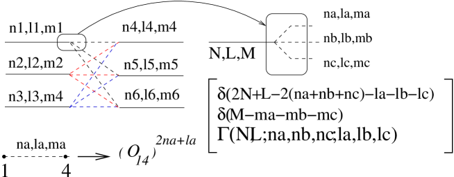
Figure 4.  : Graphical rules diagram for compact operator $\hat{O}$ representation in term of $3\otimes 3$ clusters: The exterior legs correspond to incoming and outgoing clusters in a given spectral decomposition,i.e if we choose an harmonic oscillator Hilbert space then a k particles cluster $C(1,...k)=\sum c_{1}^{n1,l1m1}...c_{k}^{nk,lk,mk}\phi(n1,l1,m1)...\phi(nk,lk,mk)$, with the $\phi$’s being harmonic oscillator wave functions. The cluster representation is therefore linear in the spectral weights $c_{j}(nj,lj,mj)$. Thence it suffices to consider harmonic oscillator exterior legs; a given slashed line $\{ij\}$-connecting exterior legs i and j-correspond to the ij th ”propagator” ${\hat{O}}_{ij}={{\cal O}_{ij}}^{2n_{ij}+l_{ij}}$, with ${\cal O}_{ij}$ the ij th matrix element of jacobean representation of the operator $\hat{O}$ and $\{n_{ij},l_{ij},m_{ij}\}$, the quantum numbers flowing in that leg, appropriated to the Hilbert space ${\cal H}$ we choose to represent the clusters (usually the harmonic oscillator Hilbert space). The vertices $\Gamma$ are universal for all operators $\hat{O}$ we might be interested in, solely depending on the Hilbert space ${\cal H}$ we have chosen to for the cluster decomposition. Conservation of flowing quantum numbers $\{n,l,m\}$ are enforced at the vertices by delta functions.

In order to proceed let us enumerate the rules needed to construct a generic graphical-rules diagram associated with ${\cal O}_{C_{1},...,C^{\prime}_{m}}$. They are:

• 1. Perform cluster decomposition in term of harmonic oscillator wave functions for both incoming and outgoing clusters: i.e
  $C(1,...k)=\sum c_{1}^{n1,l1m1}...c_{k}^{nk,lk,mk}\phi(n1,l1,m1)...\phi(nk,lk,mk)$. As we have already said, a different spectral decomposition could be used but for the purposes of this talk we will only use H.O. Hilbert space.

• 2. Draw as many exterior legs as independent H.O. $\phi(ni,lj,mj)$, and label them with $\{nj,lj,mj\}$.

• 3. Connect all the exterior legs in all possible ways consistent with connecting one incoming leg with an outgoing leg. To these lines we call propagators.

• 4-Any given such propagator, connecting exterior lines i and j contributes with a number ${{\cal O}_{ij}}^{2n_{ij}+l_{ij}}$, being ${\cal O}_{ij}$ the ij th matrix element of the jacobean representation of $\hat{O}$–see Eqs. (57,58)–and $n_{ij},l_{ij},m_{ij}$ the quantum numbers flowing in that ”propagator”.

• 5. Each Vertex contributes with a number as defined in fig. 5

  

  Figure 5.  : Method to evaluate a generic vertex: Group all the ”propagators” in pairs of neighbors by the introduction of fictitious carriers of quantum numbers $n_{x},l_{x},m_{x}$ (thick lines). The function of these lines is just to bookkeep local conservation of the quantum numbers. Otherwise they play no role and are set to unity. Dashed lines correspond to the real ”propagators”. Exterior legs are represented with thin lines. The fundamental building-block vertices are depicted in the right of the figure together with their values.

• 6. Sum over all possible diagrams consistent with the conservation of quantum numbers of rule 5.

to obtain a number,

$$\langle C_{1}^{out}(1,...)...C_{M}^{out}(1,...kM)|\hat{O}|C_{1}^{in}(1,...k1)...C_{L}^{in}(1,...kL)\rangle=$$

$$=\sum c_{1;in}^{n1in,l1in,m1in}...c_{N;in}^{nNin,lNin,mNin}c_{1;out}^{n1out,l1out,m1in}...c_{N;out}^{nNout,lNout,mNout}$$

$$\langle\phi(n1in,l1in,m1in)...\phi(nNin,lNin,mNin)|\hat{O}|$$

$$\hskip 62.59596pt\phi(n1out,l1out,m1out)...\phi(nNout,lNout,mNout)\rangle=$$

$$=\sum{\cal O}(\{n1in,l1in,m1in\},...,\{nNin,lNin,mNin\};$$

$$\hskip 79.6678pt\{n1out,l1out,m1out\},...,\{nNout,lNout,mNout\})$$

$$\hskip 22.76228ptc_{1;in}^{n1in,l1in,m1in}...c_{N;in}^{nNin,lNin,mNin}c_{1;out}^{n1out,l1out,m1in}...c_{N;out}^{nNout,lNout,mNout}$$

The graphical rules evaluate the numbers

$${\cal O}(\{n1in,l1in,m1in\},...,\{nNin,lNin,mNin\}$$

$$\hskip 79.6678pt\{n1out,l1out,m1out\},...,\{nNout,lNout,mNout\}).$$

Failure to integrate in any of the jacobean coordinates, say $Q_{1}\;....\;Q_{J}$, will produce separable overlap kernels ${\cal O}(Q_{1},...Q_{J})$,

$$\sum\{c_{nQL,lQL,mQL}\}\hskip 28.45274pt{\cal O}(Q_{1},...Q_{J})=$$

$$=\sum\{c_{...}\}{\cal O}(\{n1in,l1in,m1in\}...\{nNout,lNout,mNout\})$$

$$\hskip 56.9055pt\phi_{nq1,lq1,mq1}(Q_{1})...\phi_{nQj,lQj,mQj}(Q_{J})$$

So far this looks like being an awfully complicated way to evaluate overlap kernels. Nevertheless it is for practical cases quite powerful and allows, for most cases, a mental evaluation of overlap kernels. Let us go back to examples of figure 3. Consider Pauli exchange $P^{13}$ and consider the overlap kernel ${\cal P}^{13}(R,R^{\prime})$,

$${\cal P}^{13}(R,R^{\prime})=\langle\phi_{0,0,0}(\rho_{12})\phi_{0,0,0}(\rho_{34})|P^{13}|\phi_{0,0,0}(\rho_{12})phi_{0,0,0}(\rho_{34})\rangle$$ (62)

The graphical-rules diagram associated with Eq. (62) is given in fig. (6),

Figure 6.  : A simple application of the graphical rules. No propagators are allowed connecting the $\rho$ lines because of vertex conservation. Because we have no propagators the vertices are all equal to unity. Notice that because $P_{R,\;R^{\prime}}^{13}=0$-See Eq.57- we have the same separable potential no mater what quantum numbers flow in the line RR’

and produces an overlap kernel

$${\cal P}^{13}(R,\;R^{\prime})={\cal P}^{13}_{\{[0]_{I,II,III,IV};{\color[rgb]{0,1,0}[n,l,m],[n^{\prime},l^{\prime},m^{\prime}]}\}}\phi_{0,0,0}({\color[rgb]{0,1,0}R})\;\phi_{0,0,0}({\color[rgb]{0,1,0}R^{\prime}}),$$ (63)

with ${\cal P}^{13}_{\{[0]_{I,II,III}...\}}=1$ regardless of the quantum numbers n,l,m (or n’,l’,m’) flowing in the line RR’.

The rearrangement case is also quite simple. This time consider a p-wave in the relative coordinate between Cluster $C_{III}$ and the fourth particle. Assume ground state H.O for clusters I and II.

Figure 7.  : Rearrangement overlap. Contrary to the $P^{13}$ case we have flow of quantum numbers in the line RR’. Because we do not have more than one propagator coalescing in either external line we still have all the vertices equal to unity

The rearrangement kernel of fig.3, ${\cal R}_{3}^{II,III}(R,R^{\prime\prime})$, is given by,

$${\cal R}_{3}^{II,III}(R,\;R^{\prime\prime})={\cal R}^{\{[0]_{I},[0]_{II},[0]_{III};{\color[rgb]{0,1,0}[0,1,0]_{I,II},[0,1,0]_{III,IV}}\}}\;\phi_{0,1,0}({\color[rgb]{0,1,0}R})\;\phi_{0,1,0}({\color[rgb]{0,1,0}R^{\prime\prime}})$$ (64)

with ${\cal R}^{\{[0]_{I}...\}}=1/\sqrt{3}$-see Fig. 7. Suppose now that we have plane waves between both Cluster I and II and cluster III and particle 4. We have to decompose the spectra of these plane waves with the help of the formula,

$$e^{(k\cdot r)}=e^{(i(\beta k)\cdot(\beta r)/\beta^{2}}={\left[2\pi\beta^{2}\right]}^{3/2}\;\sum i^{2n+l}\phi_{n,l,m}^{\left[\beta\right]}(\beta k)\;{\phi_{n,l,m}^{\left[\beta\right]}}^{*}(\beta r)$$ (65)

to obtain,

$$\int d^{3}R\;d^{3}R^{\prime\prime}\;e^{(ik\cdot R)}{\cal R}_{3}^{II,III}(R,R^{\prime\prime})e^{-(ik^{\prime}\cdot R^{\prime\prime})}=$$

$$\hskip 85.35826pt{\left[2\pi\beta^{2}\right]}^{3}\;\phi_{n,l,m}^{\beta}(\beta k)\{\frac{1}{\sqrt{3}}\}^{2n+l}\phi_{n,l,m}^{\beta}(\beta k^{\prime})$$ (66)

where $\beta$ represents the cluster sizes. For different cluster sizes the above spectral analysis is more complicated but still linear on the spectra and can also be worked out. However this further complication is not important for this talk. It is important to notice that because the rearrangement operator is compact this series converges with powers of $\{\frac{1}{\sqrt{3}}\}^{2n+l}$. This is a general feature of compact operators and in practice few terms are sufficient for a good approximation. It is important to notice that the topology of graphical-rules diagrams do not depend on a particular Hilbert space decomposition of clusters. Different decompositions yield different vertex and different values for the propagators but the rules will stay the same. In this talk I will not pursue this issue any longer.

We have come a long way and are now able to discuss transition potentials. As we will see this method of graphical rules allows one to extract physical consequences, even in the absence of a quantitative model for hadron interactions. For some applications of the graphical rules see [10].

6.1 The OZI ${}^{3}P_{0}$ insertions

Back in the OZI era [11], it was realized that hadronic decay must be realized through the creation (and annihilation) of $q-\bar{q}$ pairs. The reason was that these pairs carried the vacuum quantum numbers. A quantitative description of this creation was not available and still evades us at the present. The ${}^{3}P_{0}$ mechanism for hadronic decay is depicted in the figure 8.

Figure 8.  : The ${}^{3}P_{0}$ for hadronic decay. In some region of space a ${}^{3}P_{0}$ $q-\bar{q}$ is created and the quarks are rearranged to belong to different mesons $M_{2}$, and $M_{3}$.

In the absence of any robust, first-principles, theoretical description of the ${}^{3}P_{0}$ mechanism, we would like to know at least the answer to two basic questions:

• what is the strength of the ${}^{3}P_{0}$ creation and

• where it is created.

The first idea is to fit both parameters and hope for these fitted parameters to stay put when we hop from reaction to reaction. For an example see ref.[12]. The shortcoming of such approach is that we do not have a model for these transition potentials which do (as it is clear by now) change from sector to sector. It is a matter of principle, and a crucially important one, that hadronic models, albeit deemed successful in one or another aspect should be exportable to a variety of hadronic phenomena which were, at first glance and prior to the model application, unrelated with each other. For instance: decay and exotic scattering.

Therefore we would like to contemplate a situation where we have only to deal at most with one scale: the size of hadrons. This scale can be thought to be the scale of the effective force among quarks. The rest should come from geometrical overlaps and group theory. This was the philosophy I held when coming from RGM calculations (NN repulsive core) I landed at Nijmegen and tried to understand how I could extend RGM calculation to transition potentials. My answer to the above two questions was to set up the diagrammatic approach of the graphical-rules to overlap kernels.

Let us consider figure 8 and think backward in time. In the remote past we had two mesons $M_{2}$ and $M_{3}$ which approach each other until another configuration becomes possible for color singlets: A meson M1 and ${}^{3}P_{0}$ quark-antiquark pair. By now we understand this amplitude to be the familiar exchange kernel. We still had to answer the two above questions about both the size of the ${}^{3}P_{0}$ pair and the whereabouts of such creation. It turns out that we can dump both these two parameters in one single parameter. Let us see how this happens.

Consider the creation of the ${}^{3}P_{0}$ pair in one point of space. We have

$${\cal P}(\rho_{12},R^{\prime})=\langle...^{3}P_{0}(\rho_{34})\delta(R-a)|P^{13}|M_{2}(\rho_{12})M_{3}(\rho_{34})...\rangle.$$ (67)

For simplicity in Eq.(67) we only wrote the relevant clusters and assume from now on the intervening clusters to be given by single H.O wave functions of the same size (if this is not the case then we must work with H.O. spectral decomposition of these clusters, an unessential complication-see Eqs.(6,6)). Using $\delta(R-a)=\sum\phi_{n,l,m}(a)\phi_{n,l,m}(R)$ we get for the overlap of fig. 8,

$${\cal P}^{a}_{\{a;n1,l1,m1,n6,l6,m6\}}(\rho_{12},R^{\prime})=$$

$$\hskip 17.07182pt\sum{\color[rgb]{1,0,1}\phi_{n3,l3,m3}(a)}\phi_{n1,l1,m1}(\rho_{12})\phi_{n6,l6,m6}(R^{\prime})$$

$$\hskip 22.76228pt{\cal P}^{13}(\{n1,l1,m1\},\{n2,l2,m2\},\{{\color[rgb]{1,0,1}n3,l3,m3}\},...,\{n6,l6,m6\})$$

$$\hskip 28.45274pt\langle M_{2}(\rho_{12})|\phi_{n4,l4,m4}\rangle\langle M_{3}(\rho_{34})|\phi_{n5,l5,m5}\rangle$$

$$\hskip 34.14322pt\langle M_{1}(\rho_{12})|\phi_{n1,l1,m1}\rangle\;\langle^{3}P_{0}|\phi_{n2,l2,m2}\rangle$$

But it turns out that the numbers ${\cal P}^{13}(\{n1,l1,m1\},...,\{n6,l6,m6\})$ go to zero very fast with increasing n, l, m. Furthermore it happens that in general the intervening mesons $M_{1},\;M_{2},\;M_{3}$ can, to good accuracy, be approximated by H.O. wave functions with a given size, so that in general ${\cal P}^{a}_{\{a;...\}}(\rho_{12},R^{\prime})$ is given by,

$${\cal P}^{a}_{\{a;...\}}(\rho_{12},R^{\prime})\simeq{\color[rgb]{1,0,1}\phi_{000}(a)}$$

$$\hskip 8.5359pt{\cal P}^{13}(\{n1,l1,m1\},\{0,1,m\},\{{\color[rgb]{1,0,1}000}\},...,\{000\},\{n6,l6,m6\})$$

$$\hskip 14.22636pt\phi_{n1,l1,m1}(\rho_{12})\phi_{n6,l6,m6}(R^{\prime})$$ (69)

Notice that the arbitrary distance a gets transformed in a multiplicative constant $\phi_{000}(a)$ which can be absorbed in the overall strength $V_{o}$ of the transition potential. A similar conclusion would have been obtained for space distributions other than $\delta(\rho_{34}-a)$ with new multiplicative constants now different from $\phi_{000}(a)$. In fig. 9 we draw the graphical-rules diagram to evaluate one such overlap kernels. We have (we omit the $l_{z}$ component),

Figure 9.  : Basic diagram for scalar decay. The bare scalar must contain a coordinate-space wave function with L=1. This is because quarks and antiquarks have opposite intrinsic parity. So we must have to internal propagator with L=1 which can only couple to n=1 or L=2. The decay process is dominated by the N=1,L=0 case

$${\cal V}_{T}(\rho_{12},R^{\prime\prime})=V_{o}IS\;{\cal P}^{13}_{\{[0,1],[0,1],[0],[0];{\color[rgb]{0,1,0}[0],[1,0]}\}}\phi_{0,1}(\rho_{12}))\phi_{1,0}({\color[rgb]{0,1,0}R^{\prime\prime}})$$

$${\cal V}_{T}(\rho_{12},R^{\prime\prime})=V_{o}\;IS\;{\cal P}^{13}_{\{[0,0],[0,1],[0],[0];{\color[rgb]{0,1,0}[0],[0,1]}\}}\phi_{0,0}(\rho_{12}))\phi_{0,1}({\color[rgb]{0,1,0}R^{\prime\prime}})$$ (70)

for, respectively, scalar and vectorial decay. IS stands for the product of group 9-J symbols for trivial spin and isospin exchanges. $V_{o}$ stands for the strength of ${}^{3}P_{0}$ creation which is deemed universal. We see that we have different overlap kernels, depending on the particles involved, with all related with one another by a single unknown parameter $V_{o}$.

Equipped with this formalism we have studied the scalar sector. This will be the subject of the next section.

The first thing to notice is that overlap kernels (transition potentials) are non-local and therefore any local approximation to these potentials must be, not only energy dependent, but also process dependent, i.e depending not only on the the sector we are studying (scalar, vectorial, and so on…) but also on the cluster sizes. The simplest way to construct such local approximations is to perform a delta shell fitting of these non-local potentials for phenomenological studies. Although numerically useful those parameters have no special physical significance.

6.2 Scalar decays

We want to solve a set of coupled channel equations

$$H=$$

$$\;\left[\begin{array}[]{cc}\includegraphics[width=51.21504pt]{umcanal.eps}&\includegraphics[width=136.5733pt]{sigmadecay.eps}\\ \includegraphics[width=136.5733pt]{sigmadecay.eps}&\includegraphics[width=51.21504pt]{doiscanais.eps}\end{array}\right]$$ (73)

The quark and the antiquark in the permanently closed scalar channel move in relative P-waves due to the fact that quarks and antiquarks have opposite intrinsic parity. On the other hand the coupled mesonic channels have relative wave functions which can be at most S and D waves. The ${}^{3}P_{0}$ provide another source of $L=1$ angular momentum. In 1986, [13], we have used harmonic oscillator quark forces although by now it should be clear that the spatial form of the transition potential cannot change much with different quark confining forces. Of course, for different quark kernels like, for instance, linear confinement, the overall potential strength may change so as to have reasonable hadronic sizes and a correct hadronic size is the only ingredient necessary to have a correct spatial dependence of the transition potential. Graphical-rules diagrams were used to calculate a set of overlap kernels -see Eq. (6.1)-for simple examples. We still had a universal constant $V_{o}$ which was kept fixed for all decays.

In that paper, equation (6.2) was given by,

$$\left[-\frac{d^{2}}{dr^{2}}+\frac{L(L+1)}{r^{2}}+2\mu(E)V(r)-k^{2}(E)\right]\phi_{E}(r)=0$$ (75)

with $L,\;\mu,\;K^{2},V(E)$ $(n+m)\;(n+m)$ matrices. The matrix E and $\mu$ are given by,

$$E=\sqrt{k^{2}+m_{1}^{2}}+\sqrt{k^{2}+m_{2}^{2}},\;\mu=\frac{dk^{2}}{2dE}$$ (76)

and the effective potential by,

$$V(E)=\left[\begin{array}[]{cc}V_{c}&{\cal V}_{T}\\ {\cal V}_{T}^{trans}&V_{meson-meson}\end{array}\right]$$ (77)

A simple-minded local approximation to the geometrical overlap in $V_{T}$, i. e. a local approximation for ${\cal V}_{T}(\rho_{12},R^{\prime\prime})$ was also used in Ref. [13], by just considering the diagonal terms of ${\cal V}_{T}(\rho_{12},R^{\prime\prime})$, i.e. ${\cal V}_{T}(\rho_{12},R^{\prime\prime})\rightarrow{\cal V}_{T}(\rho_{12},R^{\prime\prime})\delta(\rho_{12}-,R^{\prime\prime})$. This simplification was not strictly necessary once finite sums of separable kernels are amenable to analytic treatment. A further simplification allowing for closed algebraic expressions for the phase shifts is obtained just by considering-because the diagonal transition overlap kernel always peaks around a definite value for $\rho=R=\rho_{0}$ for a given decay, just by considering the value of this overlap at that point. This is depicted in figure 10.

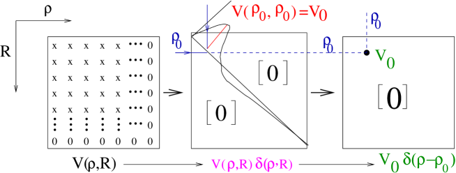
Figure 10.  : Two simple minded approximations for geometrical overlaps-See Z. Phys. C 21 in Ref. 10

But what cannot be hidden is the fact that all these local approximations merely constitute examples of as many different fits to the non-local kernels with at least two parameters:

• The relative strengths of the geometrical overlaps for different decay reactions ( for example, the numbers $IS\;{\cal P}^{13}_{\{[0,1],[0,1],[0],[0];[0],[1,0]\}}$ of Eq.(6.1)) which are given by the graphical rules and…

• …the point where the diagonal part of these overlaps is maximum ($\rho_{0}$ in fig.10).
  

Bearing this in mind, we have obtained the results presented in figure 11.

Figure 11.  : $K\pi\;\pi\pi\;\eta\pi$ invariant masses

7 Conclusions

Despite the fact that we still lack a theory, based in first principles, workable enough to describe the totality of hadronic phenomena, nature has come to our help in the form of chiral symmetry. This symmetry provides us with a sort of a filter allowing us, in what concerns low energy physics, to gloss over some details of the quark dynamics. As we have shown, the pion Goldstone boson and $\pi\;\pi$ scattering are classic examples of this filtering insofar that any quark dynamics will have led us to the same result. The price is that now we have a linkage between quark scattering and quark-antiquark creation and annihilation: They are bound to reproduce the Adler zeros. Whereas quark exchange yields repulsion quark annihilation must yield attraction in order to achieve this. This mechanism of cancellation, a consequence of chiral symmetry, is clear in $\pi\pi$ scattering. In turn, this linkage will put a boundary on how to treat hadronic coupled channels. Among all the decay reactions the scalar sector exhibits a notable property: hadronic coupled channels produce an effective extra potential in the confined sector strong enough as to have an extra pole. This effect is quite difficult to get rid of as the discussion on Graphical-rules diagrammatic evaluation of transition overlap kernels have shown us. Probably the reason why we do not see the same effect for $L\neq 0$ stems from the fact that the hadronic relative wave function inside this extra potential-which for $L\neq 0$ has also changed from the scalar one-is, due to centrifugal barrier, depleted. Finally I would like to thank the organizers for having invited me for this very agreeable conference

8 References

References

- 1. G. Jona-Lasinio and F. M. Marchetti, Phys. Lett. B 459, 208 (1999).
- 2. V. P. Gusynin, V. A. Miransky and I. A. Shovkovy, Phys. Rev. D 52, 4718 (1995); ibid, Nucl. Phys. B 462, 249 (1996); A. Chodos, K. Everding and D. A. Owen, Phys. Rev. D 42, 2881 (1990); D. Kabat, K. M. Lee and E. Weinberg, Phys. Rev. D 66, 014004 (2002).
- 3. J. E. Ribeiro, P. Bicudo Phys. Rev. D 42, 1611 (1990).
- 4. S. L Adler and A.C. Davis, Nuc. Phys. B 244 469 (1984).
- 5. J Wheeler, Phys. Rev 52, 1083 (1937).
- 6. J. E. Ribeiro Z. Phys C30, 615 (1986).
- 7. J. E. Ribeiro, P. Bicudo Phys. Rev. D 42, 1635 (1990).
- 8. P. Bicudo, S. Cotanch, F. Llanes-Estrada, P. Maris, J. E. Ribeiro, A. Szczepaniak, Phys. Rev. D 65, 076008 (2002).
- 9. J.E. Ribeiro Phys. Rev D 25, 2406 (1982)
- 10. E. Beveren Z. Phys. C17, 135 (1983); Z. Phys. C21, 291 (1984); A. Arriaga, A. M. Eiro, F.D. Santos and J.E. Ribeiro, Phis. Rev C 37, 2312 (1988).
- 11. S. Okubo, Phys Lett 5, 105 (1963); G. Zweig CERN-report Th 401,412 (1964); J. Iizuka, K. Okada, O.Shito, Prog. Theor. Phys. 35, 1061 (1966).
- 12. E. Van Beveen, G. Rupp, T. A. Rijken, and C. Dullemond, Phys Rev D. 27, 1527, (1983).
- 13. E. van Beveren T.A. Rijken, K. Metzger, C. Dullemond, G. Rupp, and J. E. Ribeiro, Z. Phys. C 30,615 (1986).