Coulomb Corrections for Coherent Electroproduction of Vector Mesons: Eikonal Approximation

Abstract

Virtual radiative corrections due to the long range Coulomb forces of heavy nuclei with charge $Z$ may lead to sizeable corrections to the Born cross section usually used for lepton-nucleus scattering processes. An introduction and presentation of the most important issues of the eikonal approximation is given. We present calculations for forward electroproduction of rho mesons in a framework suggested by the VDM (vector dominance model), using the eikonal approximation. It turns out that Coulomb corrections may become relatively large. Some minor errors in the literature are corrected. PACS. 25.30.-c Lepton induced reactions - 25.30.Rw Electroproduction reactions - 13.40.-f Electromagnetic processes and properties - 25.30.Bf Elastic electron scattering Eur. Phys. J. A (2004)
DOI 10.1140/epja/i2003-10182-3

1 Introduction

Due to the small size of the elemental electric charge $e=\sqrt{4\pi\alpha}$, it is for most electromagnetic elementary particle reactions fully sufficient to calculate only in Born approximation. But this is no longer true when heavy nuclei are involved, like e.g. lead, where the relevant perturbation expansion parameter $\alpha Z\sim 0.6$ is not small. It is then possible that even at high energies, the ratio of the exact and the Born cross section does not approach unity. One prominent example for this observation is the photoelectric effect, where a single photon knocks out an electron from the $K$ shell, or electron positron pair production by a single photon incident on a nucleus, where the electron is captured into the $K$ shell [1, 2]. For small $\alpha Z$ and high photon energy $\epsilon_{\gamma}$, the cross section for these processes is given by the Sauter formula [3]

$$\sigma_{0}\simeq 4\pi\alpha^{6}Z^{5}\lambda_{C}^{2}\frac{1}{\epsilon_{\gamma}},$$ (1)

where $\lambda_{C}$ is the electron Compton wavelength. Applying the Born approximation in the usual sense, i.e. by the use of plane waves for the positron, was attempted by Hall and Oppenheimer [4] already in 1931 in the case of the photoelectric effect. But a central difficulty in the treatment of the photoeffect arose from the distorted wave function of the ejected electron. The bound state wave function depends on $\alpha Z$ and only terms of relative order $\alpha Z$ survive in the Born matrix element. Terms of this order also come from the continuum wave function. Using exact wave functions for the continuum electron, it turns out that the cross section calculated from plane waves for the ejected electron is already wrong for small $\alpha Z$. It is therefore not astonishing that Coulomb corrections can become very large even at high energies. For the derivation of the Sauter formula, nonrelativistic bound state wave functions and approximate Sommerfeld-Maue wave functions for the ejected electron were used. Boyer [5] improved the calculation by using exact bound state wave functions and Sommerfeld-Maue wave functions for the continuum wave function. The calculational advantage of using Sommerfeld-Maue wave functions relies in the fact that the exact continuum wave functions are only available as an expansion in partial waves, and for higher energies summation over a large number of terms is necessary in order to compute exact matrix elements. But Sommerfeld-Maue wave functions are valid for the Coulomb potential of point-like charges, and hence do not take into account the finite size of the nucleus. We therefore pursue a similar strategy, namely the eikonal distorted wave approximation, where the advantage is that also finite size effects can be taken into account. This is clearly necessary for nuclear processes, whereas the relevant physical length scale of the photoelectric effect is given by $\sim(\alpha Z)^{-1}\lambda_{C}$ and much larger than a typical nuclear radius.

In the following part of this paper, we revisit the eikonal approximation by giving a condensed introduction to the subject, where we also point out the most important facts related to possible improvements concerning the range of validity of the method in its basic form. In sect. 3, we apply our calculation to coherent vector meson electroproduction. It turns out that the Coulomb corrections are indeed large for heavy nuclei, and that it is necessary to use a rather accurate description of the electrostatic nuclear potential. We correct some errors in the literature and rederive the eikonal result given in [6].

2 Eikonal Approximation

For highly relativistic particles in a potential $V$ with asymptotic momentum $\vec{p}$, one may neglect the mass of the particle ($|E-V|,|\vec{p}\,|\gg m$), such that the energy-momentum relation reduces to ($\hbar=c=1$)

$$(E-V)^{2}=\vec{p}^{\,2}+m^{2}\,\rightarrow\,E-V=p,\,p=|\vec{p}\,|.$$ (2)

The classical relation (2) for the (initial) momentum of the particle $\vec{p}_{i}=p_{i}\hat{p}_{i}$ can be taken into account approximately in quantum theory by modifying the plane wave describing the initial state of the particle by the eikonal phase $\chi_{1}(\vec{r})$

$$e^{i\vec{p}_{i}\vec{r}}\,\rightarrow\,e^{i\vec{p}_{i}\vec{r}+i\chi_{1}(\vec{r})}\,,$$ (3)

$$\chi_{1}(\vec{r})=-\int\limits_{-\infty}^{0}V(\vec{r}+\hat{p}_{i}s)ds\,.$$ (4)

If we choose the initial momentum parallel to the $z$-axis $\vec{p}_{i}=p_{z}^{i}\hat{{\bf{e}}}_{z}$, the phase is

$$\chi_{1}(\vec{r})=-\int\limits_{-\infty}^{z}V(x,y,z^{\prime})dz^{\prime}\,.$$ (5)

The $z$-component of the momentum then becomes

$$-i\partial_{z}e^{ip_{z}^{i}z+i\chi_{1}}=(p_{z}^{i}-V)e^{ip_{z}^{i}z+i\chi_{1}},$$ (6)

and further analysis shows that also the transverse momentum modification is well approximated. Analogously, for the final state wave function follows

$$e^{i\vec{p}_{f}\vec{r}-i\chi_{2}(\vec{r})},$$ (7)

where

$$\chi_{2}(\vec{r})=-\int\limits_{0}^{\infty}V(\vec{r}+\hat{p}_{f}s^{\prime})ds^{\prime}\,.$$ (8)

For the sake of simplicity, we consider spinless particles first. The spatial part of the free charged particle current

$$-ie[e^{-i\vec{p}_{f}\vec{r}}\vec{\nabla}e^{i\vec{p}_{i}\vec{r}}-(\vec{\nabla}e^{-i\vec{p}_{f}\vec{r}})e^{i\vec{p}_{i}\vec{r}}]=e(\vec{p}_{i}+\vec{p}_{f})e^{i(\vec{p}_{i}-\vec{p}_{f})\vec{r}}$$ (9)

becomes

$$-ie[e^{-i\vec{p}_{f}\vec{r}+i\chi_{2}(\vec{r})}\vec{\nabla}e^{i\vec{p}_{i}\vec{r}+i\chi_{1}(\vec{r})}-(\vec{\nabla}e^{-i\vec{p}_{f}\vec{r}+i\chi_{2}(\vec{r})})e^{i\vec{p}_{i}\vec{r}+i\chi_{1}(\vec{r})}]=$$

$$e(\vec{p}_{i}+\vec{p}_{f}+\vec{\nabla}\chi_{1}-\vec{\nabla}\chi_{2})e^{i(\vec{p}_{i}-\vec{p}_{f})\vec{r}+i\chi(\vec{r})}\,,$$ (10)

where $e$ is the charge of the particle and $\chi(\vec{r})=\chi_{1}(\vec{r})+\chi_{2}(\vec{r})$. The spatial part of the current now contains the additional eikonal phase, and the prefactor contains gradient terms of the eikonal phase which represent essentially the change of the electron momentum due to the attraction of the electron by the nucleus.

So far we have only considered the modification of the phase of the wave function, and for many problems, like the one treated in this paper, this is a sufficient approximation. It has been applied to elastic high energy scattering of Dirac particles in an early paper by Baker [8]. However, the method leads, e.g. for quasielastic nucleon knockout scattering of electrons on lead with initial energy $\epsilon_{1}=300$ MeV and energy transfer $\omega=100$ MeV, to errors up to 50% in the calculated cross sections. The reason is that also the amplitude of the incoming and outgoing particle wave functions is changed due to the Coulomb attraction. This fact is related to the classical observation that an ensemble of negatively charged test particles approaching a nucleus is focused due to its attractive potential. For the sake of completeness, we give here a short discussion of this effect.

Knoll [9] derived the focusing from a high energy partial wave expansion, following previous results given by Lenz and Rosenfelder [10, 11]. E.g., for the incoming particle wave in the vicinity of the nucleus he obtained an approximation for the electron wave function ($u_{p}$ is the constant free electron spinor)

$$\psi_{i}=e^{i\delta_{+}}(p^{\prime}/p)e^{i\vec{p^{\prime}}\vec{r}}\{1+a_{1}r^{2}-2a_{2}\vec{p^{\prime}}\vec{r}+ia_{1}r^{2}\vec{p^{\prime}}\vec{r}+ia_{2}[(\vec{p^{\prime}}\times\vec{r})^{2}+\vec{\sigma}(\vec{p^{\prime}}\times\vec{r})]\}u_{p},$$ (11)

where $\sigma$ describes spin changing effects. A similar formula holds for the final state wave function. The so-called effective momentum $\vec{p^{\prime}}$ is parallel to $\vec{p}$ and is given by the classical momentum of the electron in the center of the nucleus, i.e. $p^{\prime}=|E-V(0)|$. The parameters $a_{1,2}$ depend on the shape of the nuclear electrostatic potential. For a homogeneously charged sphere with radius $R_{s}$ they are given by $a_{1}=-\alpha Z/6p^{\prime}R_{s}^{3},\,a_{2}=-3\alpha Z/4p^{\prime 2}R_{s}^{2}$. The increase of the amplitude of the wave while passing through the nucleus is given by the $-2a_{2}\vec{p^{\prime}}\vec{r}$-term. The $a_{1}r^{2}$-Term accounts for the decrease of the focusing also in transverse direction. Imaginary terms like $ia_{2}(\vec{p^{\prime}}\times\vec{r})^{2}$ describe the deformation of the wave front near the center of the nucleus. They could be obtained correspondingly by an expansion of the eikonal phase in that region, and $\delta_{+}$ is the eikonal phase in the center of the nucleus $\chi(0)$.

Apart from the spin structure which is absent for scalar particles, the eikonal approximation relies basically on the same strategy for particles with or without spin, namely on the modification of the wave function by the eikonal phase. But there are also gradient terms present in the expression for the spinless current (10), which lead to corrections to the current which are of comparable magnitude as those which result from the wave focusing. Such terms are not explicitly present in the Dirac expression for the current (12) below. It is instructive to have a closer look at the structure of the electron current in a potential. A Gordon decomposition of the electron current

$$j^{\mu}=e\bar{\Psi}\gamma^{\mu}\Psi$$ (12)

can be performed by using the Dirac equation $[i\gamma^{\mu}(\partial_{\mu}+ieA_{\mu})-m]\Psi=0$. The current can be split into a convective current and a spin current

$$j_{G}^{\mu}=\Biggl{\{}\frac{ie}{2m}\bigl{[}\bar{\Psi}\partial^{\mu}\Psi-(\partial^{\mu}\bar{\Psi})\Psi\bigl{]}-\frac{e^{2}}{m}\bar{\Psi}\Psi A^{\mu}\Biggr{\}}$$

$$+\frac{e}{2m}\partial_{\nu}[\bar{\Psi}\sigma^{\mu\nu}\Psi]\,,$$ (13)

which are separately conserved and gauge invariant. For exact solutions of the Dirac equation, the two forms of the current are of course equivalent. Here, the convective current has exactly the same structure as the current of a scalar particle in a potential. Kopeliovich et al. [6] calculate Coulomb corrections by describing the leptons as spinless particles. The discussion above clarifies when such an approximation is justified (see also sect. 3).

In the following, we will consider electrons with energies of the order of several GeV. Then the impact of the focusing effect on the matrix element will not be larger than about one percent even for heavy nuclei like lead, where the electrostatic potential in the center of the nucleus is ($Z=82$, $A=208$)

$$\sim\frac{3}{2}\frac{\alpha Z}{R_{A}}\sim 25\,\mbox{MeV},$$ (14)

and $R_{A}\sim 7.1$ fm is the equivalent radius of a homogeneously charged sphere, which we will call ”nuclear radius” for short in the following. E.g., for a scattering process where the initial and final momentum of the electron is of the order of $10$ GeV/c, the focusing enters the cross section by a factor of the order $(p^{\prime}/p)^{4}=(10.025/10)^{4}\sim 1.01$, according to (11).

3 Coherent Electroproduction of Vector Mesons

3.1 Matrix Element

Coherent electroproduction of vector mesons from virtual photons plays an important role in the understanding of the transition of soft diffractive models to quantum chromodynamics [12, 13]. Models based on the assumption of vector dominance have been applied successfully to describe the data [14]. Our intention is not to give a better model to describe the vector meson production, but to explore the importance of Coulomb correction effects. Therefore we use a schematic model, which captures some essential features of the production process. But it is clear that for a more realistic analysis a better model should be used.

Our model is the one proposed in [6], which is inspired by the vector dominance model and which allows to derive a relatively simple form for the vector meson production amplitude on a nucleus with mass number $A$ and nuclear charge $Z$.

We denote the energy momentum vectors of the initial and final electron by $(\epsilon_{1,2},\vec{p}_{1,2})$ and the momentum of the produced meson by $\vec{p}_{V}$. $\vec{e}_{V}$ denotes the polarization vector of the meson. The production amplitude is then given by

$$M(eA\rightarrow e^{\prime}VA)=\int\limits_{0}^{\infty}dx\,\vec{e}_{V}\cdot\vec{f}(\vec{p}_{1},\vec{p}_{2},\vec{p}_{V},x),$$ (15)

where $\vec{f}=\vec{f}_{1}-\vec{f}_{2}$ and

$$\vec{f}_{1,2}(\vec{p}_{1},\vec{p}_{2},\vec{p}_{V},x)=\frac{1}{2\omega_{1,2}}\frac{\partial}{\partial\omega_{1,2}}$$

$$\times\int\frac{d^{3}r}{r}\Bigl{\{}\Bigl{[}\epsilon_{1}\vec{p}_{2}-\epsilon_{2}\vec{p}_{1}\Bigr{]}+\Bigl{[}\epsilon_{1}\vec{\nabla}\chi_{2}(\vec{r})+\epsilon_{2}\vec{\nabla}\chi_{1}(\vec{r})\Bigr{]}\Bigr{\}}$$

$$\times\exp[i\vec{\kappa}\vec{r}+i\chi_{1}(\vec{r})+i\chi_{2}(\vec{r})-i\omega_{1,2}r].$$ (16)

For details concerning the derivation of eq. (16) we refer to [6] and the appendix of this paper. We use a different sign convention for the eikonal phase than [6]. The gradient terms are artefacts of the spinless treatment of the electrons in [6] and therefore their physical significance in eq. (16) dubious at best. However, from our discussion above follows that they can be neglected for momentum transfer $Q^{2}=(\vec{p}_{1}-\vec{p}_{2})^{2}-(\epsilon_{1}-\epsilon_{2})\gg R_{A}^{-2}$, since they are of the order of $\alpha Z/R_{A}$, and $|\epsilon_{1}\vec{p}_{2}-\epsilon_{2}\vec{p}_{1}|=\sqrt{\epsilon_{1}\epsilon_{2}Q^{2}}$.

In (16), we have

$$\omega_{1}^{2}=(1-x)(\epsilon_{1}-\epsilon_{2})^{2}-x(1-x)\vec{p}_{V}^{\,2}-2x/B,$$

$$\omega_{2}^{2}=(1-x)((\epsilon_{1}-\epsilon_{2})^{2}-m_{V}^{2})^{2}-x(1-x)\vec{p}_{V}^{\,2}-2x/B$$ (17)

and $\vec{\kappa}=\vec{p}_{1}-\vec{p}_{2}-x\vec{p}_{V}$. Note that in eq. (50) in [6], the squares for $\omega_{1,2}$ are missing and the terms containing $B$ are wrong. We give therefore a detailed derivation of eqns. (16, 17) in the appendix, which is missing in [6]. Note also the different sign in front of $\omega_{1,2}$ in the exponent. The misprints will be corrected in the electronic preprint version of the paper [7].

B is the slope parameter of the differential cross section. For coherent electroproduction, it is related to the mean charge nuclear radius squared $\langle r^{2}_{A}\rangle_{rms}$ by (see e.g. [6, 13])

$$B=\frac{1}{3}\langle r^{2}_{A}\rangle_{rms}=\frac{1}{5}R_{A}^{2}.$$ (18)

At high energies and $\epsilon_{1,2}\gg\sqrt{Q^{2}}$, the vectors $\vec{p}_{1}$, $\vec{p}_{2}$ and $\vec{p}_{1}-\vec{p}_{2}$ are nearly parallel. Therefore we choose the $z$-axis along $\vec{p}_{1}$ such that the vector $\vec{r}=(\vec{b},z)$ is given by its $z$-component and the projection $\vec{b}$ to the normal plane. Using the relation

$$\int\limits_{-\infty}^{\infty}\frac{dz}{r}e^{i\vec{\kappa}\vec{r}-i\omega r}=2K_{0}\Bigl{(}b\sqrt{\kappa_{L}^{2}-\omega^{2}}\Bigr{)},\quad$$ (19)

where $K_{0}$ is the modified Bessel function, and $\kappa_{L,T}$ the longitudinal and transverse components of $\vec{\kappa}$ with respect to $\vec{p}_{1}$, we obtain ($\chi=\chi_{1}+\chi_{2}$)

$$\vec{f}_{1,2}=\frac{\epsilon_{1}\vec{p}_{2}-\epsilon_{2}\vec{p}_{1}}{\omega_{1,2}}\frac{\partial}{\partial\omega_{1,2}}\int\limits_{0}^{\infty}db\int\limits_{0}^{2\pi}d\varphi K_{0}\Bigl{(}b\sqrt{\kappa_{L}^{2}-\omega_{1,2}^{2}}\Bigr{)}e^{i\kappa_{T}b\cos(\varphi)+i\chi(b)}$$ (20)

Eq. (19) is valid also for $\kappa_{L}^{2}-\omega^{2}<0$, whereas in [6] the sign in front of $\omega$ is problematic. From

$$\int\limits_{0}^{2\pi}d\varphi e^{i\kappa_{T}b\cos(\varphi)}=2\pi J_{0}(\kappa_{T}b),\quad\frac{\partial}{\partial z}K_{0}(z)=-K_{1}(z)$$ (21)

follows

$$\vec{f}_{1,2}=\frac{2\pi(\epsilon_{1}\vec{p}_{2}-\epsilon_{2}\vec{p}_{1})}{\sqrt{\kappa_{L}^{2}-\omega_{1,2}^{2}}}\int\limits_{0}^{\infty}db\,bK_{1}\Bigl{(}b\sqrt{\kappa_{L}^{2}-\omega_{1,2}^{2}}\Bigr{)}J_{0}(\kappa_{T}b)e^{i\chi(b)}.$$ (22)

Kopeliovich et al. [6] performed calculations for a model potential

$$V_{mono}(r)=-\frac{\alpha Z}{r}e^{-\lambda r}(1-e^{-\mu r}),$$ (23)

with an infrared cutoff $\exp(-\lambda r)$, and the last factor corresponds to the monopole form of the nuclear form factor via

$$\mu^{-2}=\frac{\langle r^{2}_{A}\rangle_{rms}}{6}.$$ (24)

The eikonal phase can be calculated analytically for such a potential. One obtains

$$\chi(\vec{r})=\chi_{1}(\vec{r})+\chi_{2}(\vec{r})=-\int\limits_{-\infty}^{\infty}dz\,V_{mono}(\vec{b},z)=$$

$$2\alpha Z\Bigl{\{}K_{0}(\lambda b)-K_{0}[(\mu+\lambda)b]\Bigr{\}}.$$ (25)

We checked the result given in Fig. 4 in [6] for small $\lambda$. Our results show the same behavior, although we obtain slightly smaller Coulomb corrections. This might be due to the fact that the authors used formula (18) only for their Sommerfeld-Maue calculations [7]. We can reproduce a nearly identical curve (Fig. 1), if we reduce the slope parameter $B$ according to formula (18) by a factor of 2.

For the nuclear radius $R_{A}$ we used the formula

$$R_{A}=(1.128\,\mbox{fm})A^{1/3}+(2.24\,\mbox{fm})A^{-1/3},$$ (26)

which is a good approximation for $A>20$, whereas the mass number and charge are related by

$$Z=\frac{A}{1.98+0.015\,A^{2/3}}.$$ (27)

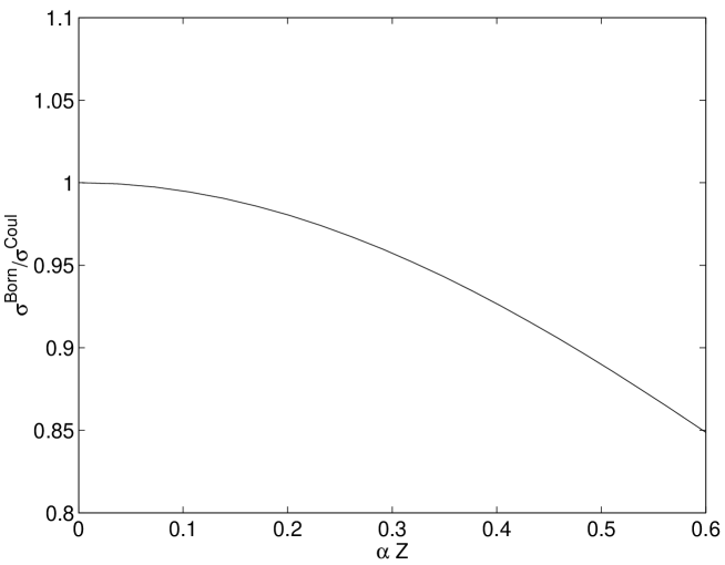
Figure 1: Coulomb correction for forward production for the model potential used in [6], calculated for $\epsilon_{1}=100$ GeV, $y=(\epsilon_{1}-\epsilon_{2})/\epsilon_{1}=0.6$, and electron scattering angle $1^{o}$ $(Q^{2}\sim 1.2\,\mbox{GeV}^{2})$, with the slope parameter replaced by $B\rightarrow B/2$ (see text).

3.2 Improved Electrostatic Nuclear Potential

It is obvious that the potential given by eq. (23) provides only an inaccurate description of the electrostatic nuclear potential near the nucleus. We looked therefore for potentials which allow an analytic calculation of the eikonal phase ($\chi$ and $\chi_{1,2}$ as well). This is not a trivial problem, since the class of meaningful analytic potentials which allow to express the eikonal phase by known special functions is rather restricted.

A good choice is a potential energy for electrons of the form

$$(\alpha Z)^{-1}V_{model}(r)=-\frac{r^{2}+\frac{3}{2}R^{2}}{(r^{2}+R^{2})^{3/2}}-\frac{24}{25\pi}\frac{R^{2}R^{\prime}r^{4}}{(r^{2}+R^{\prime 2})^{4}}\,,$$ (28)

which goes over into a Coulomb potential for $r\rightarrow\infty$, and being close to the potential generated by the relatively homogeneous spherical charge distribution of a nucleus. The charge density

$$\rho(r)=-\frac{1}{er}\partial^{2}_{r}(rV_{model}(r))$$ (29)

corresponding to (28) satisfies

$$\langle\rho\rangle=eZ\,,$$ (30)

$$\langle r^{2}\rho\rangle=\frac{3}{5}R^{2}eZ\,,$$ (31)

i.e. we can identify $R^{2}$ with the equivalent radius of the homogeneously charged sphere which is given approximately by the formula given above. $R^{\prime}$ serves as an additional fit parameter. A good choice is $R^{\prime}=0.5174R$.

Because the eikonal phase turns out to be divergent for a Coulomb-like potential, we regularize the eikonal phase by subtracting a screening potential $V_{scr}\sim(r^{2}+a^{2})^{-1/2}$ from (28), such that the potential falls off like $r^{-2}$ for large $r$. The divergence can then be absorbed in a constant divergent phase $\sim\log(a)$ without physical significance, when the limit $a\rightarrow\infty$ is taken. It is instructive to calculate the eikonal phase for the simple screened potential

$$V(r)=-\frac{\alpha Z}{\sqrt{r^{2}+R^{2}}}\,,\quad V^{a}(r)=-\frac{\alpha Z}{\sqrt{r^{2}+R^{2}}}+\frac{\alpha Z}{\sqrt{r^{2}+a^{2}}}\,.$$ (32)

One obtains for a particle incident parallel to the z-axis with impact parameter $b$ ($r^{2}=b^{2}+z^{2}$)

$$\chi_{1}^{a}=\alpha Z\int_{-\infty}^{z}dz\,\Bigl{(}\frac{1}{\sqrt{r^{2}+R^{2}}}-\frac{1}{\sqrt{r^{2}+a^{2}}}\Bigr{)}=$$

$$\alpha Z\log\frac{(z+\sqrt{z^{2}+b^{2}+R^{2}})(b^{2}+a^{2})}{(z+\sqrt{r^{2}+a^{2}})(b^{2}+R^{2})},$$ (33)

and therefore for the regularized eikonal phase

$$\chi_{1}=\lim_{a\to\infty}(\chi_{1}^{a}-\alpha Z\log(a))=\alpha Z\log\Bigl{(}\frac{z+\sqrt{r^{2}+R^{2}}}{b^{2}+R^{2}}\Bigr{)}.$$ (34)

For a simple potential $\sim(r^{2}+R^{2})^{-1/2}$, the rms radius does not exist, since the corresponding charge distribution does not fall off fast enough.

For the potential $V_{model}$ (28), the regularized eikonal phase is given by

$$(\alpha Z)^{-1}\chi(b)=\log\Bigl{(}\frac{R^{2}+b^{2}}{R^{2}}\Bigr{)}-\frac{R^{2}}{R^{2}+b^{2}}-\frac{3}{50}\frac{R^{2}R_{1}(R_{1}^{4}+4R_{1}^{2}b^{2}+8b^{4})}{(R_{1}^{2}+b^{2})^{7/2}}$$ (35)

The $z$-dependent formulae for $\chi_{1,2}$ are a bit lengthy, but can be derived in a straightforward manner.

In Fig. 2, we compare the potentials generated by eq. (23), the potential $V_{hcs}$ of a homogeneously charged sphere with radius $R_{A}$ and our model potential (28) for ${}^{208}Pb$ with identical mean squared radii in all three cases.

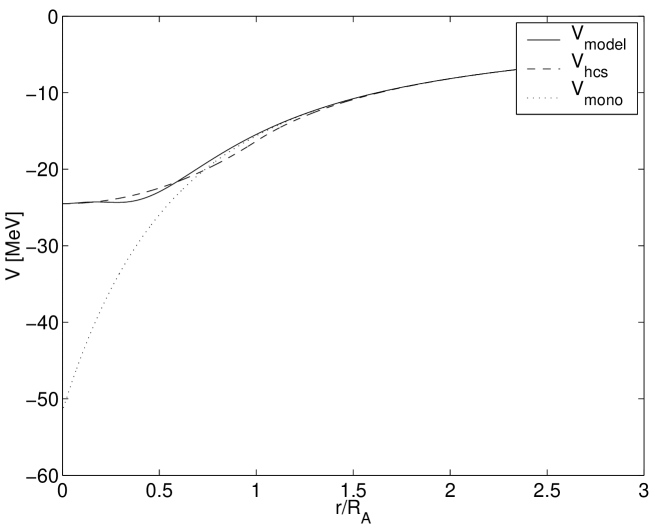
Figure 2: Comparison of different model potentials used in the calculations.

4 Results and Conclusions

For the results presented in Figs. 3-5, we used the same kinematic conditions as for Fig. 1. Fig. 3 compares the eikonal correction, using the simple model potential $V_{mono}$ and the potential $V_{model}$ given by eq. (28). It turns out that the Coulomb corrections are overestimated by the model potential given by eq. (23). This is probably due to the fact that the potential is too deep in the central nuclear region. It is therefore mandatory to use an accurate description for the nuclear Coulomb potential in order to obtain reliable results for the Coulomb corrections.

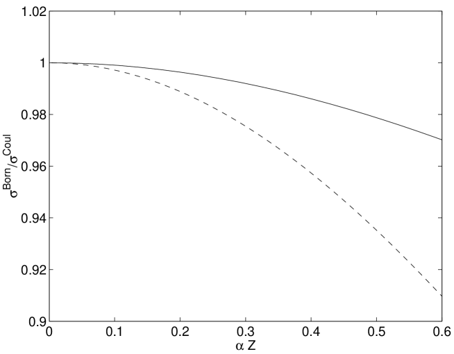
Figure 3: Comparison of Coulomb corrections for different potentials, given by eq. (28), solid line, and eq. (23), dashed line. Equal rms radii were used in both cases.

Fig. 4 shows the Coulomb corrections for each element with slope parameter $B$ according to eq. (18), but with three different rms charge radii for the electrostatic potential: the correct rms radius $\sqrt{\langle}r^{2}_{A}\rangle_{rms}$, a too large rms radius $2\sqrt{\langle}r^{2}_{A}\rangle_{rms}$ and a too small rms radius $\frac{1}{2}\sqrt{\langle}r^{2}_{A}\rangle_{rms}$. The figure clearly indicates that the distortion of the electron waves is stronger for a small nucleus, whereas for a larger nucleus, the eikonal phase varies less over the length scale given by the nuclear radius (or slope parameter). The initial and final state wave function resembles then more a plane wave in the vicinity of the nucleus. The strong dependence of the Coulomb corrections on the size of the nuclear radius clearly indicates that the use of Sommerfeld-Maue wave functions would lead to incorrect results.

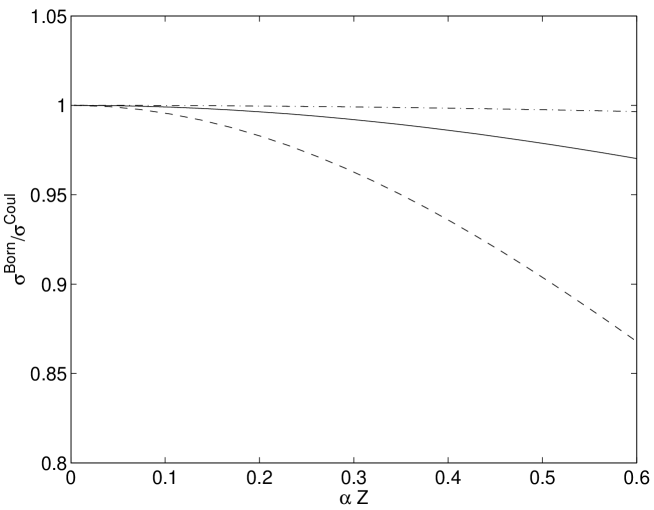
Figure 4: Coulomb corrections for the correct rms radius (solid line), doubled radius (dash-dotted), and radius divided by 2 (dashed).

The dependence of the results on the slope parameter is displayed in Fig. 5 for ${}^{208}Pb$. There we varied the slope parameter $B\rightarrow\lambda B$ for $\lambda=0.4\ldots 1.6$, where $B$ is the theoretical value given by eq. (18). The results show a clear dependence of the Coulomb corrections on the model for the hadronic current.

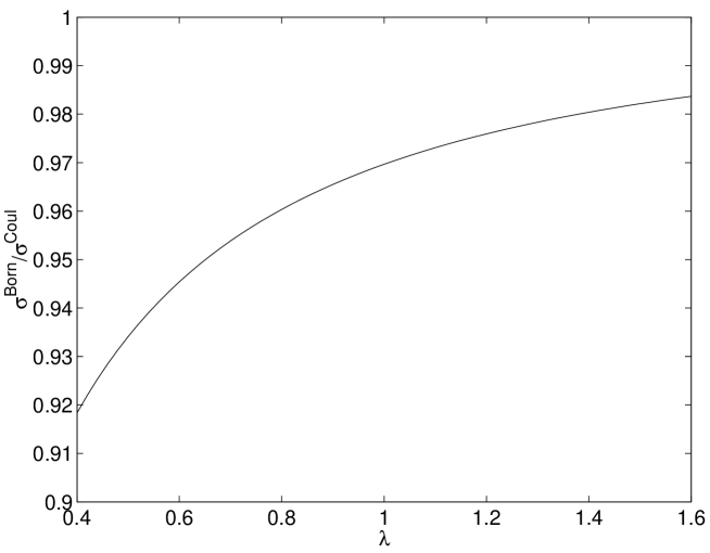
Figure 5: Coulomb corrections for different values $\lambda B$ of the slope parameter for ${}^{208}Pb$.

Finally, Fig. 6 shows the dependence of the Coulomb corrections for ${}^{16}O$ and ${}^{208}Pb$, where we have varied artificially the nuclear charge of the two elements, while the correct charge radius of the two nuclei and the corresponding slope parameter were held fixed.

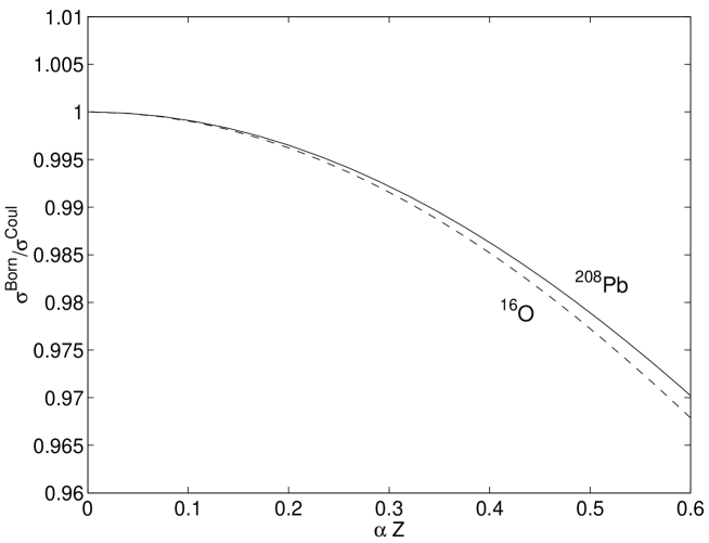
Figure 6: Dependence of Coulomb corrections on the nuclear charge, but with approximately correct nuclear radii according to eq. (26) and correct slope parameter for lead and oxygen.

The calculations presented in this paper treat only the case where the scattering angle of the electron is small, such that the expression for the vector meson production amplitude can be reduced to a simple two-dimensional integral, which can be solved without involving large computational efforts. But it is also possible to perform numerical calculations of the three-dimensional integral representation of the amplitude on a modern workstation, such that arbitrary scattering angles and more general models of the hadronic current could be treated. This is the subject of a forthcoming paper.

The oscillatory behavior of the corrected cross section shown in Fig. 3 in [6] can not be reproduced by our calculations. Fig. 4 shows clearly how important it is to use the correct charge distribution of the nucleus for the calculation of Coulomb corrections. Approximate wave functions for pointlike nuclei are therefore not adequate.

5 Appendix A. Matrix Element for Electroproduction of Vector Mesons

We start from the amplitude for coherent electroproduction of vector mesons by electrons derived in [6], eq. (27), working with the Born approximation first

$$M\propto\int\frac{d^{3}q}{Q^{2}+i0}\Bigl{[}\vec{j}(\vec{q})-j_{0}(\vec{q})\frac{\vec{q}}{\nu}\Bigr{]}\vec{J}(Q,\vec{p}_{V}).$$ (36)

where $\vec{j}$ is the spatial operator of the electron current, $\vec{J}$ the hadronic current operator, $\nu=\epsilon_{1}-\epsilon_{2}$ and $Q^{2}=\vec{q}^{\,2}-\nu^{2}$. From current conservation

$$\nu j_{0}(\vec{q})=\vec{q}\cdot\vec{j}(\vec{q})$$ (37)

we obtain

$$M\propto 2\frac{\epsilon_{1}\vec{p}_{2}-\epsilon_{2}\vec{p}_{1}}{\epsilon_{1}-\epsilon_{2}}\int\frac{d^{3}q}{\vec{q}^{\,2}-\nu^{2}}\vec{J}(Q,\vec{p}_{V}).$$ (38)

Using the hadronic model current ($\vec{\Delta}=\vec{q}-\vec{p}_{V}$ here)

$$\vec{J}(Q,\vec{p}_{V})=\frac{\vec{e}_{V}m_{V}^{2}}{m_{V}^{2}+Q^{2}}\frac{1}{1+B\vec{\Delta}^{2}/2}$$ (39)

the amplitude becomes in Born approximation

$$M\propto 2\frac{(\epsilon_{1}\vec{p}_{2}-\epsilon_{2}\vec{p}_{1})\vec{e}_{V}}{\epsilon_{1}-\epsilon_{2}}\int d^{3}r\int d^{3}q\frac{1}{(\vec{q}^{\,2}-\nu^{2})(\vec{q}^{\,2}-\nu^{2}+m_{V}^{2})}\frac{(2/B)m_{V}^{2}}{(2/B+\vec{\Delta}^{2})}e^{i(\vec{p}_{1}-\vec{p}_{2}-\vec{q})\vec{r}}\,.$$ (40)

Going over to the eikonal approximation, we modify the electron current by the eikonal phases. Therefore, we have to evaluate the integral

$$I=m_{V}^{2}\int d^{3}r\int\frac{d^{3}q}{(\vec{q}^{\,2}-\nu^{2})(\vec{q}^{\,2}-\nu^{2}+m_{V}^{2})(2/B+\vec{\Delta}^{2})}e^{i(\vec{p}_{1}-\vec{p}_{2}-\vec{q})\vec{r}+i\chi_{1}(\vec{r})+i\chi_{2}(\vec{r})}.$$ (41)

Due to the trivial identity

$$\frac{m_{V}^{2}}{Q^{2}(Q^{2}+m_{V}^{2})}=\frac{1}{Q^{2}}-\frac{1}{Q^{2}+m_{V}^{2}},$$ (42)

we can decompose integral $I=I_{1}+I_{2}$ according to

$$I_{1}=\int d^{3}r\int\frac{d^{3}q}{(\vec{q}^{\,2}-\nu^{2})(2/B+\vec{\Delta}^{2})}e^{i(\vec{p}_{1}-\vec{p}_{2}-\vec{q})\vec{r}+i\chi_{1}(\vec{r})+i\chi_{2}(\vec{r})},$$

$$I_{2}=\int d^{3}r\int\frac{d^{3}q}{(\vec{q}^{\,2}-\nu^{2}+m_{V}^{2})(2/B+\vec{\Delta}^{2})}e^{i(\vec{p}_{1}-\vec{p}_{2}-\vec{q})\vec{r}+i\chi_{1}(\vec{r})+i\chi_{2}(\vec{r})}.$$ (43)

With Feynman’s trick

$$\frac{1}{\alpha\beta}=\int\limits_{0}^{1}\frac{dx}{[\alpha x+\beta(1-x)]^{2}}$$ (44)

follows for $I_{1}$ first

$$I_{1}=\int\limits_{0}^{1}dx\int d^{3}r\int d^{3}q\frac{e^{i(\vec{p}_{1}-\vec{p}_{2}-\vec{q})\vec{r}+i\chi_{1}(\vec{r})+i\chi_{2}(\vec{r})}}{[(\vec{q}^{\,2}-\nu^{2})(1-x)+(2/B+(\vec{q}-\vec{p}_{V})^{2})x]^{2}}=$$

$$\int\limits_{0}^{1}dx\int d^{3}r\int d^{3}q\frac{e^{i(\vec{p}_{1}-\vec{p}_{2}-\vec{q})\vec{r}+i\chi_{1}(\vec{r})+i\chi_{2}(\vec{r})}}{[(\vec{q}-x\vec{p}_{V})^{\,2}-x^{2}\vec{p}_{V}^{2}-(1-x)\nu^{2}+2x/B+x\vec{p}_{V}^{\,2}]^{2}}.$$ (45)

Shifting the integration variable $\vec{q}\rightarrow\vec{q}+x\vec{p}_{V}$ leads to

$$I_{1}=\int\limits_{0}^{1}dx\int d^{3}r\int d^{3}q\frac{e^{i(\vec{p}_{1}-\vec{p}_{2}-x\vec{p}_{V}-\vec{q})\vec{r}+i\chi_{1}(\vec{r})+i\chi_{2}(\vec{r})}}{[\vec{q}^{\,2}-(1-x)\nu^{2}+x(1-x)\vec{p}_{V}^{\,2}+2x/B]^{2}}=$$

$$\frac{1}{2}\int\limits_{0}^{1}dx\int d^{3}r\frac{1}{\omega_{1}}\frac{\partial}{\partial\omega_{1}}\int d^{3}q\frac{e^{i(\vec{p}_{1}-\vec{p}_{2}-x\vec{p}_{V}-\vec{q})\vec{r}+i\chi_{1}(\vec{r})+i\chi_{2}(\vec{r})}}{\vec{q}^{\,2}-\omega_{1}^{2}}.$$ (46)

Finally, the identity

$$\int d^{3}q\frac{e^{-i\vec{q}\vec{r}}}{\vec{q}^{\,2}-\omega_{1}^{2}}=\pi\frac{e^{-i\omega_{1}r}}{r}$$ (47)

immediately gives the final result in agreement with eq. (16)

$$I_{1}=\int\limits_{0}^{1}dx\frac{\pi}{2\omega_{1}}\frac{\partial}{\partial\omega_{1}}\int\frac{d^{3}r}{r}e^{i(\vec{p}_{1}-\vec{p}_{2}-x\vec{p}_{V})\vec{r}-i\omega_{1}r+i\chi(\vec{r})}.$$ (48)

For $I_{2}$ we must simply replace $\nu^{2}\rightarrow\nu^{2}-m_{V}^{2}$.

References

• [1] A. Aste, K. Hencken, D. Trautmann, G. Baur, Phys. Rev. A50, 3980 (1994).
• [2] C. K. Agger, A. H. Sorensen, Phys. Rev. A55, 402 (1997).
• [3] F. Sauter, Ann. Phys. (Leipzig) 11, 454 (1931).
• [4] H. Hall, J. R. Oppenheimer, Phys. Rev. 38, 57-70 (1931).
• [5] R. H. Boyer, Phys. Rev. 117, 475 (1960).
• [6] B. Z. Kopeliovich, A. V. Tarasov, O.O. Voskresenskaya, Eur. Phys. J. A11, 345 (2001).
• [7] B. Z. Kopeliovich, private communication; see also hep-ph/0105110.
• [8] A. Baker, Phys. Rev. B134, 240 (1964).
• [9] J. Knoll, Nucl. Phys. A223, 462 (1974).
• [10] F. Lenz, thesis, Freiburg, Germany, 1971.
• [11] F. Lenz, R. Rosenfelder, Nucl. Phys. A176, 513 (1971).
• [12] A. Donnachie, P.V. Landshoff, Phys. Lett. B348, 213 (1995).
• [13] T. Renk, G. Piller, W. Weise, Nucl. Phys. A689, 869 (2001).
• [14] T.H. Bauer, R.D. Spital, D.R. Yennie, F.M. Pipkin, Rev. Mod. Phys. 50, 261 (1978), Erratum-ibid. 51, 407 (1979).