hep-ph/0312030
KIAS–P03087,    VEC/PHYSICS/P/2/2003-2004 Supersymmetric threshold corrections to $\Delta m^{2}_{\odot}$

1 Introduction

Recent developments in neutrino experiments have provided fairly significant information on the neutrino mass and mixing parameters. The new analysis of Super-Kamiokande collaboration indicates that the atmospheric neutrino mass-squared difference and mixing angle satisfy $\Delta m^{2}_{A}=1.3-3.0$ eV² and $\sin^{2}2\theta_{A}>0.9$ [1]. A global analysis of all solar neutrino data yields $\Delta m^{2}_{\odot}=7.1^{+1.2}_{-0.6}\times 10^{-5}$ eV² and $\theta_{\odot}=32.5^{+2.4}_{-2.3}$ degrees including the KamLAND [2] and SNO salt results [3]. One of the important unknowns in the neutrino sector is the structure of absolute mass scales which cannot be determined by oscillation experiments. For this we can turn to neutrino-less double beta decay experiments, cosmological bounds on neutrino masses such as the WMAP bound and so on as explained next.

If neutrinos are almost degenerate (that is the mass splitting is negligible compared to the masses), they could lead to an observational signature in the future nuclear or astrophysical/cosmological experiments. At present, there are several upper limits on the absolute neutrino mass scale. Tritium $\beta$ decay experiments put $m_{\beta}<2.2$ eV [4], and neutrino-less double beta decay experiments constrain the effective Majorana mass; $|m_{ee}|<0.3-1.3$ eV depending on the uncertainty in the nuclear matrix element [5]. The WMAP collaboration has drawn the impressive limit on the sum of three neutrino masses, $\sum_{i}m_{i}<0.71$ eV, or equivalently, $m_{i}<0.23$ for three degenerate neutrinos [6]. However, the cosmological bounds are based on some assumptions and models, depending on which one sets $\sum_{i}m_{i}<1.1$ or $2.12$ eV [7].

The nearly degenerate neutrino mass pattern is vulnerable to quantum corrections. Its stability has been studied extensively in the context of the see-saw mechanism where the renormalization group evolution (RGE) [8, 9] can produce too large corrections to keep the required mass degeneracy [10]. Apart from the RGE effect, there can be another type of quantum corrections, the low energy threshold effect.

For a sizable threshold corrections, one needs a large Yukawa coupling effect or a large splitting between slepton masses in supersymmetric theories. The latter can arise in SO(10) models with the top quark coupling effect on the RGE from the Planck scale to the GUT scale [11] or in a minimal supersymmetric standard model (MSSM) with non-universal soft terms [12]. The general computation of the threshold corrections in the Standard Model and in the MSSM has been made in [13]. Note that the threshold corrections can arise independently of the RGE effect in the seesaw mechanism and thus should be present in any mechanism of generating the neutrino mass matrix [14]. This corrections to neutrino masses are generated by loop corrections.

In this paper, we will consider the low energy threshold corrections in the MSSM with minimal flavour violation, where the flavour dependent structure arise only from the usual Yukawa couplings and thus the supersymmetry breaking is taken to be flavour blind. This is usually assumed in the MSSM to avoid the dangerous supersymmetric flavour problems. Two popular scenarios of such are the minimal supergravity (mSugra) model and the gauge mediated supersymmetry breaking (GMSB) models [15]. The sources of sizable threshold corrections are the tau Yukawa coupling and the slepton mass splitting driven by it. As a consequence, we find that the solar neutrino mass splitting can arise solely through the threshold effect or constrains some parameter space where $\tan\beta$ and the scalar and gaugino soft masses are large.

Our consideration readily applies to low energy models of neutrino masses in which almost degenerate mass eigenvalues are generated by some mechanism around the electroweak scale. Our results are independent of the form of neutrino mass textures, while they depend on the pattern of eigenvalues. Note that degenerate eigenvalues can be obtained from many different mass textures. Therefore, in this article we do not highlight how a specific texture is obtained from a definite flavor symmetry. If we invoke a specific flavor symmetry our result will be less generally valid and therefore weaker. We also find it is easier to motivate degenerate neutrino mass spectrum from an experimental point of view in view of latest experimental results[1, 2, 3].

We give a few examples now to motivate our calculations event hough details of mass texture generation is beyond the scope of the present article.

(a) The simplest possibility is to invoke a suitable Yukawa texture, for instance, of the dimension-five operator ${f_{ij}\over M_{R}}L_{i}L_{j}\langle H\rangle\langle H\rangle$ in the see-saw mechanism with a suitable low mass scale of right handed neutrino $\nu_{R}$ namely $M_{R}$.

(b) Alternatively, one could consider a low energy Higgs triplet as the origin of neutrino mass generation [16], in which the resulting flavour violating signatures can be probed in the future experiments, event hough our RGE analysis needs to be modified in the presence of $SU(2)$ triplet scalars. (c) More natural framework of generating a degenerate mass matrix is to impose certain flavor symmetries at low energy [18], sometimes realizing texture-zeros [19]. Some models existing in literature can be non-supersymmetric. However, it is rather straightforward to implement supersymmetry in such models[17]. Therefore we do not foresee serious problems if flavour scale is around the electroweak scale, as long as the flavor symmetry is either a global symmetry or a discrete symmetry.

If neutrino mass texture is generated at a sufficiently high scale, one has to consider as well the RGE effect which typically gives a larger correction than the threshold effect. For example, in the usual see-saw mechanism, the RGE contribution is given by $I_{\tau}\approx{h^{2}_{\tau}\over 16\pi^{2}}\log{M_{R}\over M_{S}}$ where $M_{S}$ is the supersymmetry breaking scale. For $\tan\beta\sim 50$, $M_{S}=M_{Z}$ and $M_{R}\sim 10^{10}$ GeV, we get $I_{\tau}\sim 0.02$ which is an order of magnitude larger than our threshold corrections as we will see later. The threshold corrections will also be useful if in some case RGE effects cancel tree level mass generated at high scale. A typical example can be found in a class of models for the radiative amplification of the mixing angles, in which case the degeneracy of three masses should be stronger at the electroweak scale than at a high scale [20].

2 Radiative corrections to $\Delta m^{2}_{\odot}$

Let us consider a tree-level neutrino mass matrix $M^{0}$ which has eigenvalues $m^{0}_{i}$ and the mixing matrix $U^{0}$. In the tree-level mass basis, the one-loop corrected mass matrix takes the form,

$$M_{ij}=m^{0}_{i}\delta_{ij}+{1\over 2}I_{ij}(m^{0}_{i}+m^{0}_{j}).$$ (1)

where $I_{ij}$ is the one-loop factor coming from wave-function renormalization. It is often convenient to calculate radiative corrections in the flavour basis where the charged lepton masses are diagonal. Denoting the one-loop factor as $I_{\alpha\beta}$ in the flavour basis, we have the relation,

$$I_{ij}=\sum_{\alpha,\beta}I_{\alpha\beta}U^{0}_{\alpha i}U^{0}_{\beta j}\,.$$ (2)

In the case of the minimal flavour violation in the MSSM, only the diagonal components $I_{\alpha\alpha}$ are non-vanishing and they satisfy $I_{ee}=I_{\mu\mu}\neq I_{\tau\tau}$. The difference between $I_{ee,\mu\mu}$ and $I_{\tau\tau}$ arises from the sizable tau Yukawa coupling and the mass splitting between the 3rd generation sleptons and the others. The equality $I_{ee}=I_{\mu\mu}$ is deviated by the small electron and muon Yukawa couplings which can be safely ignored. Then, one has

$$I_{ij}=I_{ee}\delta_{ij}+I_{\tau}\,U^{0}_{\tau i}U^{0}_{\tau j}$$ (3)

where $I_{\tau}\equiv I_{\tau\tau}-I_{ee}$. The overall factor $I_{ee}$ can be dropped out and only $I_{\tau}$ can modify the tree level result.

When the neutrino masses are nearly degenerate, $m^{0}_{1}\simeq m^{0}_{2}\simeq m^{0}_{3}\simeq m_{\nu}$, the quantum correction $I_{\tau}$ may break up the degeneracy in a significant way. The change in the mass eigenvalues can be approximated by $m_{i}-m^{0}_{i}\simeq m_{i}^{0}I_{ii}$ and thus we get

$$\Delta m^{2}_{ij}\simeq\Delta{m^{0}_{ij}}^{2}+2m_{\nu}^{2}(I_{ii}-I_{jj})\,.$$ (4)

Considering the mass-squared difference $\Delta m^{2}_{12}$ for the solar neutrino oscillation, one finds that the loop correction can produce the desired mass splitting if

$$I_{\tau}\simeq{\Delta m^{2}_{\odot}\over 2\cos 2\theta_{\odot}s_{A}^{2}m_{\nu}^{2}}$$ (5)

where we have taken the standard parameterization of the mixing matrix $U^{0}$; $U_{\tau 1}=s_{12}s_{23}$ and $U_{\tau 2}=c_{12}s_{23}$ identifying $\theta_{12}=\theta_{\odot}$ and $\theta_{23}=\theta_{A}$ to a good approximation of $\theta_{13}\ll 1$. Here, we remark that the above contribution arises since the solar neutrino mixing is not maximal [10]. Recall that $\cos 2\theta_{\odot}=0.35-0.49$. From the observed values of the neutrino mass and mixing parameters mentioned in the Introduction, one finds that the range of

$$I_{\tau}=(1.1-3.7)\times 10^{-3}\left(0.3\mbox{ eV}\over m_{\nu}\right)^{2}$$ (6)

is acceptable to generate solar neutrino mass-squared difference. With the best-fit values, we get $I_{\tau}\simeq 1.9\times 10^{-3}$ for $m_{\nu}=0.3\mbox{ eV}$.

On the other hand, the threshold correction has to be constrained so that $I_{\tau}<3.7\times 10^{-3}(0.3\mbox{ eV}/m_{\nu})^{2}$, barring the cancellation between the tree-level and one-loop contributions. This consideration will put some constraint on the MSSM parameter space if $m_{\nu}>0.3$ eV. Therefore if we start from a high energy theory such as mSugra or GMSB, and evolve the supersymmetry breaking mass parameters from the high energy theory to the low energy, we can identify high energy parameter space for which the solar mass splitting $m^{2}_{\odot}$ becomes too large compared to the currently measured LMA region.

In this paper, we will assume no CP violation, that is, vanishing CP phases in neutrino mass matrix. The RGE studies showed that both the mixing angles and mass eigenvalues can be affected by the presence of phases [21]. Similar phenomenon is expected to occur with threshold corrections, which we will leave for a future study.

3 Supersymmetric threshold corrections with minimal flavour violation

In the MSSM with minimal flavour violation, the low energy threshold correction is solely determine by the quantity $I_{\tau}\equiv I_{\tau\tau}-I_{ee}$ defined in Eq. (3). The explicit formulae for the threshold corrections have been obtained in Ref. [13]. Adopting its result, we calculate $I_{\tau}$ which consists of three contributions from the charged Higgs boson, neutralinos and charginos as follows.

Charged-Higgs contribution

$$16\pi^{2}I_{\tau}(H^{\pm})={g^{2}\over 2}{m_{\tau}^{2}\over m_{W}^{2}}\left[{1\over 4}(1+\tan^{2}\beta)(-{1\over 2}+\ln{m_{H^{\pm}}^{2}\over Q^{2}})+{1\over 2}(1+{3\over 2}\ln{m_{H^{\pm}}^{2}\over m_{W}^{2}})\right]$$ (7)

where $\tan\beta=v_{2}/v_{1}$.

Neutralino/sneutrino contribution

$$16\pi^{2}I_{\tau}(\chi^{0}(1)) = +{g^{2}+g^{\prime 2}\over 8}\sum_{j=1}^{4}(s_{W}N_{1j}-c_{W}N_{2j})^{2}$$ (8)

$$[F(m_{\chi^{0}_{j}}^{2},m^{2}_{\tilde{\nu}_{\tau}})-F(m_{\chi^{0}_{j}}^{2},m^{2}_{\tilde{\nu}_{e}})]$$

$$16\pi^{2}I_{\tau}(\chi^{0}(2)) = -{2\over v_{2}}\sqrt{g^{2}+g^{\prime 2}}\sum_{j=1}^{4}(s_{W}N_{1j}-c_{W}N_{2j})N_{4j}m_{\chi^{0}_{j}}$$ (9)

$$[G(m_{\chi^{0}_{j}}^{2},m^{2}_{\tilde{\nu}_{\tau}})-G(m_{\chi^{0}_{j}}^{2},m^{2}_{\tilde{\nu}_{e}})]$$

where $N_{ij}$ is the neutralino diagonalization matrix with the flavour index $i$ corresponding to $\tilde{B},\tilde{W}_{3},\tilde{H}^{0}_{1}$ and $\tilde{H}^{0}_{2}$ and the mass-eigenstate index $j$ for the state $\chi^{0}_{j}$. The loop functions are defined by

$$F(x,y)=\ln{y\over Q^{2}}-{1\over 2}+{x\over y-x}+{x^{2}\over(y-x)^{2}}\ln{x\over y}$$

$$G(x,y)=\ln{y\over Q^{2}}-1-{x\over y-x}\ln{x\over y}$$

Chargino/charged-lepton loop contribution

$$16\pi^{2}I_{\tau}(\chi^{\pm}(1)) = +{g^{2}\over 4}\sum_{j=1}^{2}U_{1j}^{2}[F_{j+}-F(m_{\chi^{\pm}_{j}}^{2},m_{\tilde{e}}^{2})+{m_{LL}^{2}-m_{RR}^{2}\over m_{\tilde{\tau}_{1}}^{2}-m_{\tilde{\tau}_{2}}^{2}}F_{j-}]$$ (10)

$$+{\sqrt{2}\over 4}g\sum_{j=1}^{2}U_{1j}U_{2j}{m_{\tau}^{2}(A_{\tau}-\mu\tan\beta)\over v_{1}(m_{\tilde{\tau}_{1}}^{2}-m_{\tilde{\tau}_{2}}^{2})}F_{j-}$$

$$+{1\over 2}{m_{\tau}^{2}\over v_{1}^{2}}\sum_{j=1}^{2}U_{2j}^{2}[F_{j+}-{m_{LL}^{2}-m_{RR}^{2}\over m_{\tilde{\tau}_{1}}^{2}-m_{\tilde{\tau}_{2}}^{2}}F_{j-}]$$

$$16\pi^{2}I_{\tau}(\chi^{\pm}(2)) = -{\sqrt{2}\over v_{2}}g\sum_{j=1}^{2}U_{1j}V_{2j}m_{\chi^{\pm}_{j}}[G_{j+}-G(m_{\chi^{\pm}_{j}}^{2},m_{\tilde{e}}^{2})+{m_{LL}^{2}-m_{RR}^{2}\over m_{\tilde{\tau}_{1}}^{2}-m_{\tilde{\tau}_{2}}^{2}}G_{j-}]$$ (11)

$$-{2\over v_{2}}\sum_{j=1}^{2}U_{2j}V_{2j}m_{\chi^{\pm}_{j}}{m_{\tau}^{2}(A_{\tau}-\mu\tan\beta)\over v_{1}(m_{\tilde{\tau}_{1}}^{2}-m_{\tilde{\tau}_{2}}^{2})}G_{j-}$$

where $m_{LL}$ and $m_{RR}$ denote the left-handed and right-handed stau masses whose mass eigenvalues are denoted by $m_{\tilde{\tau}_{1,2}}$, $m_{\tilde{e}}$ denotes the left-handed selectron (or smuon) mass, $U_{ij}$ and $V_{kj}$ are the chargino diagonalization matrices with the index $i=1,2$ for the flavour states $\tilde{W}^{-}$, $\tilde{H}^{-}_{1}$, $k=1,2$ for $\tilde{W}^{+}$, $\tilde{H}^{+}_{2}$, and $j=1,2$ for the mass eigenstate $\chi^{\pm}_{j}$. Two loop functions are defined by

$$F_{j\pm}={1\over 2}[F(m_{\chi^{\pm}_{j}}^{2},m_{\tilde{\tau}_{1}}^{2})\pm F(m_{\chi^{\pm}_{j}}^{2},m_{\tilde{\tau}_{2}}^{2})],$$

$$G_{j\pm}={1\over 2}[G(m_{\chi^{\pm}_{j}}^{2},m_{\tilde{\tau}_{1}}^{2})\pm G(m_{\chi^{\pm}_{j}}^{2},m_{\tilde{\tau}_{2}}^{2})].$$

Summing all the contributions, we get the total low-energy threshold correction to the neutrino mass matrix defined at the scale $Q=M_{Z}$:

$$I_{\tau}=I_{\tau}(H^{\pm})+I_{\tau}(\chi^{0}(1))+I_{\tau}(\chi^{0}(2))+I_{\tau}(\chi^{\pm}(1))+I_{\tau}(\chi^{\pm}(2)).$$

In the next section, we will analyze $I_{\tau}$ in models with minimal gravity-mediated and gauge-mediated supersymmetry breaking.

4 Results in mSugra and GMSB models

Given the tree-level neutrino mass matrix $M^{0}$ with almost degenerate eigenvalues at the weak scale, the threshold correction derived in the above section can produce a significant change in the neutrino mass splitting. As one can see from Eqs. (6-10), the low energy threshold effect arises due to the flavour violation in the Yukawa and slepton sectors. The latter is driven also by the Yukawa coupling effect in the MSSM with minimal flavour violation, we expect to have a sizable correction for large $\tan\beta$ and large soft scalar masses $A_{0}$. In GMSB also large $\tan\beta$ region gives larger contribution than small $\tan\beta$ region. However the overall corrections induced in the GMSB scenario is generally smaller than the overall correction in mSugra scenario. This is mainly because the splitting among soft masses in GMSB is relatively smaller than those of the mSugra case. For low $\tan\beta$ charged Higgs dominates in the mSugra case as can be seen from Tables 1 and 2, whereas for large $\tan\beta$, typically charged Higgs and chargino contributions are important for large $A_{0}$. In mSugra, there is a large parameter space where the desired solar neutrino mass splitting can be generated. However, for large $m_{0}$, $m_{1/2}$ and $\tan\beta$ solar splitting can be overshot and thus bounds on high energy parameter space can also be obtained. This is displayed in Figures 1 and 2. Let us note that the figures are generated by calculating some specific points connected by lines. We also see $A_{0}$ dependence of the result is very mild. Results also do not depend appreciably on the sign of $A_{0}$. For the soft masses less than 1 TeV and $\tan\beta\leq 50$, we find $I_{\tau}<4\times 10^{-3}$, which is marginally compatible with the limit $I_{\tau}<3.7\times 10^{-3}(0.3\mbox{ eV}/m_{\nu})^{2}$. Stronger bounds can be put for $m_{\nu}>0.3$ eV. In GMSB we typically have much small effect. Therefore GMSB parameter space is generally compatible with the solar neutrino data in the sense that chances of generating the solar splitting $\Delta m^{2}_{\odot}$ is much smaller in the GMSB case than the mSugra case. These results are given in Table 3.

In doing these calculations we have used SOFTSUSY program [22] to calculate the low energy supersymmetry breaking soft parameters in mSugra as well as GMSB scenarios of supersymmetry breaking.

5 Conclusion

If neutrino masses are almost degenerate, quantum corrections can give rise to a significant effect on the neutrino mass and mixing parameters. One of important radiative corrections is the low energy threshold effect which has to be added to the tree-level mass matrix defined at the weak scale. In this paper, we have considered such threshold corrections in the context of the minimal supergravity and and gauge-mediated supersymmetry breaking models where the lepton flavour violation arises only through the usual Yukawa coupling effect. At low energy, there are two sources of threshold corrections; the tau Yukawa coupling and the slepton mass splitting driven by it. In mSugra models, these two effects become important to determine the solar neutrino mass splitting when both the scalar and gaugino soft masses and $\tan\beta$ are large. As a consequence, the threshold correction can provide a radiative origin of the solar neutrino mass splitting or some constraints on the mSugra parameter space if the overall neutrino mass scale is observed near the current cosmological limit; $m_{\nu}\sim 0.3$ eV. However we must keep in mind that these numerical bounds can potentially be much stronger if $m_{\nu}>0.3$ eV. The effect turns out to be suppressed in the GMSB models for typical ranges of parameter spaces at the high energy scale.

Acknowledgments: B.B. would like to thank Korea Institute for Advanced Study for very kind hospitality and financial support for one month. B.B. and E.J.C. would like to thank the organizers of WHEPP-7 workshop where this work was initiated. We would also like to thank Prof. Asim K. Ray for some discussions on neutrino textures.

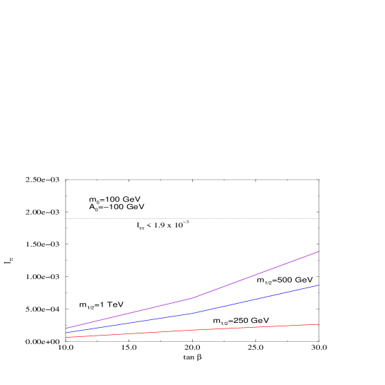
Figure 1: Total amount of $I_{\tau}$ is plotted as a function of $\tan\beta$. We have chosen three representative values of $m_{1/2}=250,500,1000$ GeVs respectively. We have restricted ourselves up to $\tan\beta=30$ because tachionic modes appear for larger $\tan\beta$. For such small values of $m_{0},m_{1/2}$, total $I_{\tau}$ remains within acceptable limits

CASE	mSugra parameters				$I_{\tau}(H^{\pm})$	$I_{\tau}(\chi^{0})$	$I_{\tau}(\chi^{\pm})$	Total=$I_{\tau}$
	$m_{0}$	$m_{1/2}$	$A_{0}$	$\tan\beta$
1	100	250	-100	10	6.0 $\times 10^{-5}$	-2.7 $\times 10^{-7}$	4.1 $\times 10^{-6}$	6.38 $\times 10^{-5}$
2	100	250	-100	20	2.2 $\times 10^{-4}$	-1.8 $\times 10^{-5}$	-2.4 $\times 10^{-5}$	1.78 $\times 10^{-4}$
3	100	250	-100	30	4.5 $\times 10^{-4}$	7.1 $\times 10^{-4}$	-1.2 $\times 10^{-4}$	1.04 $\times 10^{-3}$

Table 1: This table shows the break-up of $I_{\tau}$ for typical values of mSugra parameters and displays individual contributions from individual $H^{\pm},\chi^{0}$ and $\chi^{\pm}$ loops. For $m_{0}\sim 100$ GeV tachionic modes appear for large $\tan\beta\sim 40$.

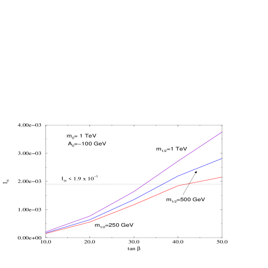
Figure 2: For large $\tan\beta$ threshold corrections can produce $\Delta m^{2}_{\odot}$ to fit LMA solution and put bounds on soft parameter space, in particular for $\tan\beta>50$. The dotted line corresponds to the best fit value of $\Delta m^{2}_{\odot}$ for the approximately degenerate neutrino mass $m_{\nu}=0.3$ eV.

CASE	mSugra parameters				$I_{\tau}(H^{\pm})$	$I_{\tau}(\chi^{0})$	$I_{\tau}(\chi^{\pm})$	Total=$I_{\tau}$
	$m_{0}$	$m_{1/2}$	$A_{0}$	$\tan\beta$
1	1000	1000	-100	30	1.1 $\times 10^{-3}$	3.3 $\times 10^{-5}$	5.4 $\times 10^{-4}$	1.67 $\times 10^{-3}$
2	1000	1000	-100	40	1.8 $\times 10^{-3}$	6.5 $\times 10^{-5}$	8.9 $\times 10^{-4}$	2.75 $\times 10^{-3}$
3	1000	1000	-100	50	2.4 $\times 10^{-3}$	1.1 $\times 10^{-4}$	1.2 $\times 10^{-3}$	3.71 $\times 10^{-3}$

Table 2: This table shows the break-up of $I_{\tau}$ for values of mSugra parameters $m_{0}=1000,m_{1/2}=1000,A_{0}=-100$ and displays individual contributions from individual $H^{\pm},\chi^{0}$ and $\chi^{\pm}$ loops.

CASE	GMSB parameters				$I_{\tau}(H^{\pm})$	$I_{\tau}(\chi^{0})$	$I_{\tau}(\chi^{\pm})$	Total=$I_{\tau}$
	$N_{5}$	$M_{mess}$	$\Lambda$	$\tan\beta$
1	1	1.61 $\times 10^{5}$	7.6 $\times 10^{4}$	10	6.4 $\times 10^{-5}$	-9.5 $\times 10^{-7}$	2.7 $\times 10^{-5}$	9.0 $\times 10^{-5}$
2	1	1.61 $\times 10^{5}$	7.6 $\times 10^{4}$	20	2.4 $\times 10^{-4}$	-3.6 $\times 10^{-6}$	5.7 $\times 10^{-5}$	2.9 $\times 10^{-4}$
3	1	1.61 $\times 10^{5}$	7.6 $\times 10^{4}$	30	5.0 $\times 10^{-4}$	-8.0 $\times 10^{-6}$	9.8 $\times 10^{-5}$	5.9 $\times 10^{-4}$
4	1	1.61 $\times 10^{5}$	7.6 $\times 10^{4}$	40	8.9 $\times 10^{-4}$	-8.0 $\times 10^{-6}$	2.0 $\times 10^{-4}$	1.0 $\times 10^{-3}$
5	1	1.61 $\times 10^{5}$	7.6 $\times 10^{4}$	50	1.0 $\times 10^{-3}$	-2.0 $\times 10^{-5}$	8.0 $\times 10^{-5}$	1.1 $\times 10^{-3}$

Table 3: GMSB models produce $\Delta m^{2}_{\odot}$ which are fully consistent with the LMA region. $I_{\tau}$ and individual contributions are displayed in a typical GMSB model with the messenger sector at around $10^{5}$ GeV or so. We see that even at $\tan\beta=50$ the total $I_{\tau\tau}$ is well below the acceptable limits.

References

- [1] Super-Kamiokande Collaboration, Y. Fukuda et. al., Phys. Rev. Lett. 81 (1998) 1562; Y. Itow, talk presented at International Conference on Flavor Physics, Oct. 6-11, 2003, Seoul.
- [2] KamLAND Collaboration, K. Eguchi et. al., Phys. Rev. Lett. 90 (2003) 021802.
- [3] SNO Collaboration, S.N. Ahmed et. al., hep-ex/0309004. SK/SNO, KamLAND
- [4] Mainz, C. Weinheimer et. al., Phys. Lett. B460 (1999) 219; Troitsk, V.M. Lobashev et. al., Phys. Lett. B460 (1999) 227.
- [5] H.V. Klapdor-Kleingrothaus et. al., Eur. Phys. J. C12 (2001) 147; IGEX, C.E. Aalseth et. al, Phys. Rev. D65 (2002) 092007.
- [6] WMAP Collaboration, C.L. Bennett et. al., astro-ph/0306207.
- [7] S. Hannestad, JCAP 0305 (2003) 004; O. Elgaroy and O. Lahav, JCAP 04 (2003) 004.
- [8] P.H. Chankowski and Z. Płuciennik, Phys. Lett. B316 (1993) 312; K.S. Babu, C.N. Leung and J. Pantaleone, Phys. Lett. B319 (1993) 191; S. Antusch, M. Drees, J. Kersten, M. Lindner and M. Ratz, Phys. Lett. B519 (2001) 238.
- [9] M. Tanimoto, Phys. Lett. B360 (1995) 41; J. Ellis, G.K. Leontaris, S. Lola and D.V. Nanopoulos, Eur. Phys. J. C9 (1999) 389; P.H. Chankowski, W. Królikowski and S. Pokorski, Phys. Lett. B473 (2000) 109; N. Haba, Y, Matsui and N. Okamura, Prog. Theor. Phys. 103 (2000) 807; S.F. King, N.N Singh, Nucl. Phys. B591 (2000) 3; M-C. Chen, K.T. Mahanthappa, Int. J. Mod. Phys. A16 (2001) 3923; S. Chang, T.K. Kuo, Phys. Rev. D66 (2002) 111302; S. Antusch, J. Kersten, M. Lindner, M. Ratz, hep-ph/0305273.
- [10] J. Ellis and S. Lola, Phys. Lett. B458 (1999) 310; J.A. Casas, J.R. Espinosa, A. Ibarra and I. Navarro, Nucl. Phys. B556 (1999) 3; B569 (2000) 82; R. Barbieri, G.G. Ross and A. Strumia, hep-ph/9906470; N. Haba and N. Okamura, Eur. Phys. J. C14 (2000) 347; E. Ma, J. Phys. G25 (1999) L97.
- [11] E.J. Chun and S. Pokorski, Phys. Rev. D62 (2000) 053001.
- [12] P.H. Chankowski, A. Ioannisian, S. Pokorski and J.W.F. Valle, Phys. Rev. Lett. 86 (2001) 3488; E.J. Chun, Phys. Lett. B505 (2001) 155.
- [13] P.H. Chankowski and P. Wasowics, Eur. Phys. J. C23 (2002) 249.
- [14] For a review of the quantum corrections to the neutrino mass matrix, see, P.H. Chankowski and S. Pokorski, Int. J. Mod. Phys. A17 (2002) 575.
- [15] For a review and more references, see S.P. Martin, hep-ph/9709356.
- [16] E.J. Chun, K.Y. Lee and S.C. Park, Phys. Lett. B566 (2003) 142; D. Aristizabal Sierra, M. Hirsch, J.W.F. Valle, A. Villanova del Moral, Phys. Rev. D68 (2003) 033006; M. Senami and K. Yanamoto, hep-ph/0305203.
- [17] For general discussions see, F. Borzumati, K. Harmaguchi, Y. Nomura, T. Yanagida, hep-ph/0012118 ; F. Borzumati, Y. Nomura, Phys. Rev. D64 (2001), 053005.
- [18] R. Barbieri, L.J. Hall, G.L. Kane and G.G. Ross, hep-ph/9901228; E. Ma and G. Rajasekharan, Phys. Rev. D64 (2001) 113012; E. Ma, Phys. Rev. D66 (2001) 117301; K.S. Babu, E. Ma and J.W.F. Valle, Phys. Lett. B552 (2003) 207.
- [19] R. Barbieri, L.J. Hall and A. Strumia, Phys. Lett. B445 (1999) 407; P.H. Frampton, S.L. Glashow, D. Marfatia, Phys.Lett. B536 (2002) 79; P.H. Frampton, M.C. Oh and T. Yoshikawa, Phys. Rev. D66 (2002) 033007.
- [20] K.R.S. Balaji, A. Dighe, R.N. Mohapatra and M.K. Parida, Phys. Rev. Lett. 84 (2000) 5034; Phys. Lett. B481 (2000) 33; R.N. Mohapatra, M.K. Parida, G. Rajasekaran, hep-ph/0301234
- [21] J.A. Casas, J.R. Espinosa, A. Ibarra and I. Navarro, Nucl. Phys. B573 (2000) 652. N. Haba, Y. Matsui and N. Okamura, Eur. Phys. J. C17 (2000) 513. S. Antusch, J. Kersten, M. Lindner and M. Ratz, Nucl. Phys. B674 (2003) 401.
- [22] B.C. Allanach, Comput. Phys. Commun. 143, 305 (2002), hep-ph/0104145.