Abstract

We explore the impact of the data from the KamLAND experiment in constraining neutrino mass and mixing angles involved in solar neutrino oscillations. In particular we discuss the precision with which we can determine the the mass squared difference $\Delta m^{2}_{\odot}$ and the mixing angle $\theta_{\odot}$ from combined solar and KamLAND data. We show that the precision with which $\Delta m^{2}_{\odot}$  can be determined improves drastically with the KamLAND data but the sensitivity of KamLAND to the mixing angle is not as good. We study the effect of enhanced statistics in KamLAND as well as reduced systematics in improving the precision. We also show the effect of the SNO salt data in improving the precision. Finally we discuss how a dedicated reactor experiment with a baseline of 70 km can improve the $\theta_{\odot}$  sensitivity by a large amount.

1 Introduction

Two very important results in the field of neutrino oscillations were declared in year 2002. The first data from the neutral current(NC) events from Sudbury Neutrino Observatory(SNO) experiment were announced in April 2002 [1] Comparison of the the NC event rates with the charged current(CC) event rates established the presence of $\nu_{\mu}/\nu_{\tau}$ component in the solar $\nu_{e}$ flux reinforcing the fact that neutrino oscillation is responsible for the solar neutrino shortfall observed in the Homestake, SAGE, GALLEX/GNO, Kamiokande and SuperKamiokande experiments. The global analysis of solar neutrino data picked up the Large Mixing Angle (LMA) MSW as the preferred solution [2]. The smoking-gun evidence came in December 2002 when the KamLAND experiment reported a distortion in the reactor anti-neutrino spectrum corresponding to the LMA parameters [3]. The induction of the KamLAND data in the global oscillation analysis resulted in splitting the allowed LMA zone in two parts (at 99% C.L.) – low-LMA lying around $\Delta m_{\odot}^{2}=7.2\times 10^{-5}~{}{\rm eV^{2}}$, $\sin^{2}\theta_{\odot}=0.3$, and high-LMA with $\Delta m_{\odot}^{2}=1.5\times 10^{-4}~{}{\rm eV^{2}}$, $\sin^{2}\theta_{\odot}=0.3$ respectively. The low-LMA solution was preferred statistically by the data [4]. The recently announced SNO data from the salt-phase [5] has further disfavoured high-LMA and it now appears at $>$ 99.13% C.L. [6]. Thus the SNO and KamLAND results have heralded the birth of the precision era in the measurement of solar neutrino oscillation parameter. In this article we take a closer look at the precision with which we know the solar neutrino oscillation parameters at present and critically examine how precisely they can be measured with future data.

2 Oscillation Parameters from solar neutrino data

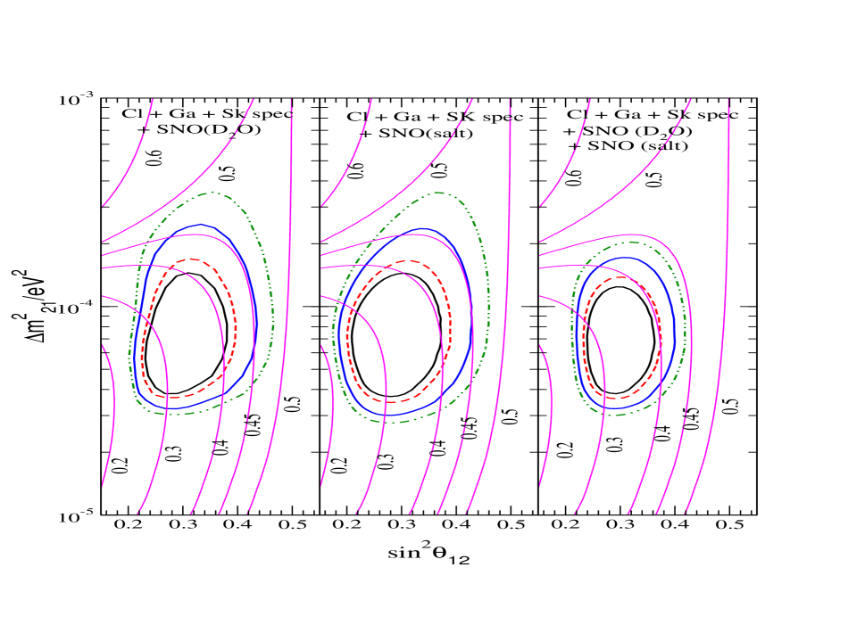
Figure 1: The 90%, 95%, 99% and 99.73% C.L. allowed regions in the $\mbox{$\Delta m_{21}^{2}$~{}}-\sin^{2}\theta_{\odot}$ plane from global $\chi^{2}$-analysis of the data from solar neutrino experiments. We use $\Delta\chi^{2}$ values to plot the C.L. contours corresponding to a two parameter fit. Also shown are the lines of constant CC/NC event rate ratio $R_{CC/NC}$.

In fig. 1 we show the impact of the SNO NC data from the pure $D_{2}O$ phase, the salt phase as well as combining the information from both phases on the oscillation parameters $\mbox{$\Delta m^{2}_{\odot}$~{}}(\equiv\mbox{$\Delta m_{21}^{2}$~{}})$ and $\sin^{2}\theta_{\odot}(\equiv\sin^{2}\theta_{12}$) from a two-flavour analysis . We include the total rates from the radiochemical experiments Cl and Ga (Gallex, SAGE and GNO combined) [7] and the 1496 day 44 bin SK Zenith angle spectrum data [8]. For the pure $D_{2}O$ phase we use the CC+ES+NC spectrum data whereas for the salt phase we use the published CC,ES and NC rates [6]. The details of the analysis procedure can be found in [9]. Also shown superposed on these curves are the isorates of the $CC/NC$ ratio. We find that
$\bullet$ The upper limit on $\Delta m^{2}_{\odot}$ tightens with the increased statistics when the salt data is added to the data from the pure $D_{2}O$ phase.
$\bullet$ The upper limit on $\sin^{2}\theta_{\odot}$ tightens. For the ${}^{8}{B}$ neutrinos undergoing adiabatic MSW transition in the sun $R_{CC}/R_{NC}\sim\sin^{2}\theta$. The SNO salt data corresponds to a lower value of the $CC/NC$ ratio which results in a shift of $\sin^{2}\theta_{\odot}$ towards smaller values.

Data	best-fit parameters		99% C.L. allowed range
set used	$\Delta m_{21}^{2}$ /($10^{-5}$eV2)	$\sin^{2}\theta_{\odot}$	$\Delta m_{21}^{2}$ /($10^{-5}$eV2)	$\sin^{2}\theta_{\odot}$
Cl+Ga+SK+$D_{2}O$	$6.06$	0.29	$3.2-24.5$	$0.21-0.44$
Cl+Ga+SK+salt	$6.08$	0.28	$3.0-23.7$	$0.19-0.43$
Cl+Ga+SK+$D_{2}O$+salt	$6.06$	0.29	$3.2-17.2$	$0.22-0.40$
Cl+Ga+SK+$D_{2}O$+KL	$7.17$	0.3	$5.3-9.9$	$0.22-0.44$
Cl+Ga+SK+$D_{2}O$+salt+KL	$7.17$	0.3	$5.3-9.8$	$0.22-0.40$

Table 1: The best-fit values of the solar neutrino oscillation parameters, obtained using different combinations of data sets. Shown also are the 99% C.L. allowed ranges of the parameters from the different analyses.

3 Impact of KamLAND data on oscillation parameters

The KamLAND detector measures the reactor antineutrino spectrum from Japanese commercial nuclear reactors situated at a distance of 80 -800 km. In this section we present our results of global two-generation $\chi^{2}$ analysis of solar+KamLAND spectrum data. For details we refer to our analysis in [4, 10] .

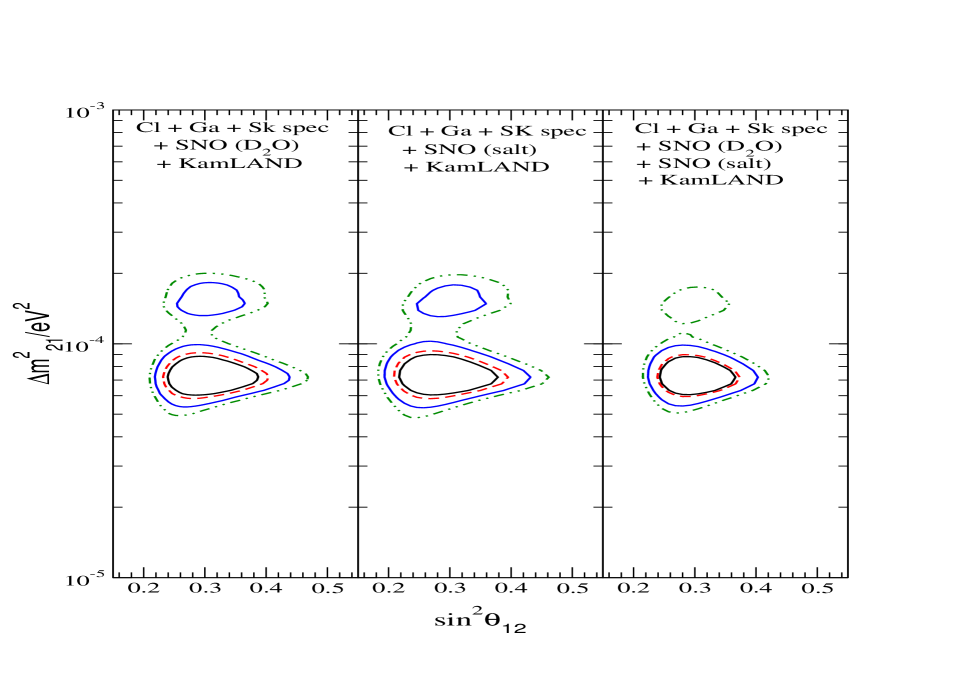
Figure 2: The 90%, 95%, 99% and 99.73% C.L. allowed regions in the $\mbox{$\Delta m_{21}^{2}$~{}}-\sin^{2}\theta_{\odot}$ plane from global $\chi^{2}$-analysis of solar and KamLAND data. We use the $\Delta\chi^{2}$ values corresponding to a 2 parameter fit to plot the C.L. contours.

Figure 2 shows the allowed regions obtained from global solar and 162 Ton-year KamLAND 
spectrum data. As is seen from the leftmost panel of figure 2 the inclusion of the KamLAND data breaks the allowed LMA region into two parts at 99% C.L.. The low-LMA region is centered around a best-fit $\Delta m^{2}_{\odot}$  of $7.2\times 10^{-5}$ eV² and the high-LMA region is centered around $1.5\times 10^{-4}$ eV². At 3$\sigma$ the two regions merge. The low-LMA region is statistically preferred over the high-LMA region. With the addition of the SNO salt data the high-LMA solution gets disfavoured at 99.13% C.L.. In Table 1 we show the allowed ranges of $\Delta m^{2}_{\odot}$  and $\sin^{2}\theta_{\odot}$ from solar and combined solar+KamLAND analysis. We find that $\Delta m^{2}_{21}$ is further constrained with the addition of the KamLAND data but $\sin^{2}\theta_{12}$ is nor constrained any further.

4 Closer look at KamLAND sensitivity

Data	99% CL	99% CL	99% CL	99% CL
set	range of	spread	range	spread
used	$\Delta m^{2}_{21}\times$	of	of	in
	10-5eV2	$\Delta m^{2}_{21}$	$\sin^{2}\theta_{12}$	$\sin^{2}\theta_{12}$
only sol	3.2 - 17.0	68%	$0.22-0.40$	29%
sol+162 Ty KL	5.3 - 9.8	30%	$0.22-0.40$	29%
sol+1 kTy KL	6.5 - 8.0	10%	$0.23-0.39$	26%
sol+3 kTy KL	6.8 - 7.6	6%	$0.24-0.37$	21%

Table 2: The range of parameter values allowed at 99% C.L. and the corresponding spread.

In Table 2 we take a closer look at the sensitivity of the KamLAND experiment to the parameters $\Delta m^{2}_{21}$ and $\theta_{12}$ with the current as well as simulated future data and examine how far the sensitivity can improve with the future data. We define the % spread in oscillation parameters as

$${\rm spread}=\frac{prm_{max}-prm_{min}}{prm_{max}+prm_{min}}\times 100$$ (1)

and determine this quantity for the current solar and KamLAND data as well as increasing the KamLAND statistics. The current systematic error in KamLAND is 6.42% and the largest contribution comes from the uncertainty in fiducial volume. This is expected to improve with the calibration of the fiducial volume and we use a 5% systematic error for 1 kTy simulated KamLAND data and 3% systematic error for 3 kTy simulated KamLAND data. The table reveals the tremendous sensitivity of KamLAND to $\Delta m^{2}_{21}$. The addition of the present KamLAND data improves the spread in $\Delta m^{2}_{21}$ to 30% from 68% obtained with only solar data. With 1 kTy KamLAND data it improves to 10% and if we increase the statistics to 3 kTy then the uncertainty in $\Delta m^{2}_{21}$ reduces to 6%. However the sensitivity of KamLAND to the parameter $\theta_{12}$ does not look as good. The addition of the current KamLAND data to the global solar analysis does not improve the spread in $\sin^{2}\theta_{12}$. With reduction of the systematic error to 5% the spread with 1 kTy statistics improves to 26% and even with a very optimistic value of 3% for the systematic uncertainty and a substantial increase of statistics to 3 kTy, the KamLAND data fails to constrain $\theta_{12}$ much better than the current solar neutrino experiments.

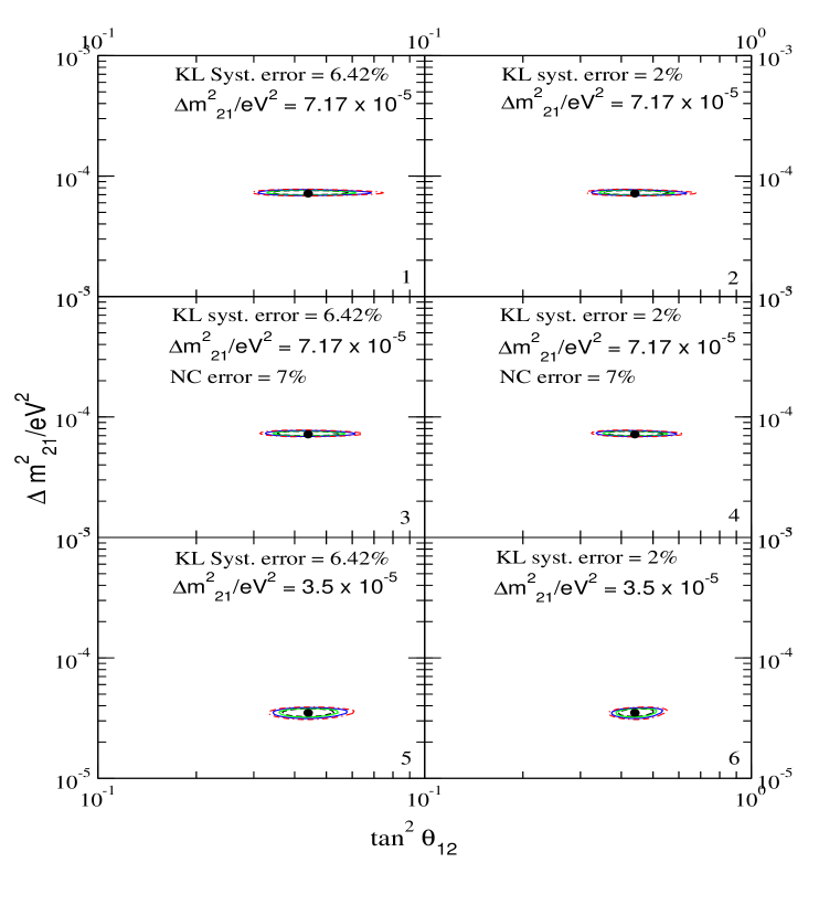
Figure 3: The contours for the combined analysis using the solar and 3 kTy simulated KamLAND spectrum. The first two rows of panels correspond to spectrum simulated at $7.2\times 10^{-5}$ eV² while the lowermost row of panels are for KamLAND data simulated at $\Delta m_{21}^{2}=3.5\times 10^{-5}$ eV².

In figure 3 we compare the allowed areas computed with spectrum simulated at $\Delta m_{21}^{2}$  = $7.2\times 10^{-5}$ eV² and $\mbox{$\Delta m_{21}^{2}$~{}}=3.5\times 10^{-5}$ eV². We show limits for the current KamLAND systematic uncertainty of 6.42% and a very optimistic systematic uncertainty of just 2%. The % spread in uncertainty for the spectrum simulated at $7.2\times 10^{-5}$ eV² with 6.42% systematic uncertainty is 37% while for $3.5\times 10^{-5}$ eV² case the spread is 25%. The effect of reducing the systematics to 2% results in the spread coming down to 32% and 19% respectively [11]. We would like to mention that the figure 3 uses the CC, NC and ES rates from the $D_{2}O$ and not the latest results from the salt phase. However the purpose of this figure is to compare the spread in $\sin^{2}\theta_{\odot}$ obtained for the two different values of $\Delta m_{21}^{2}$  and the use of the sno salt phase data is not going to change the relative spreads significantly. We also present in the middle panel of 3 the allowed areas drawn using a 7% uncertainty in the NC rate. The uncertainty in the NC rate from the $D_{2}O$(salt) phase data is 12%(9%).

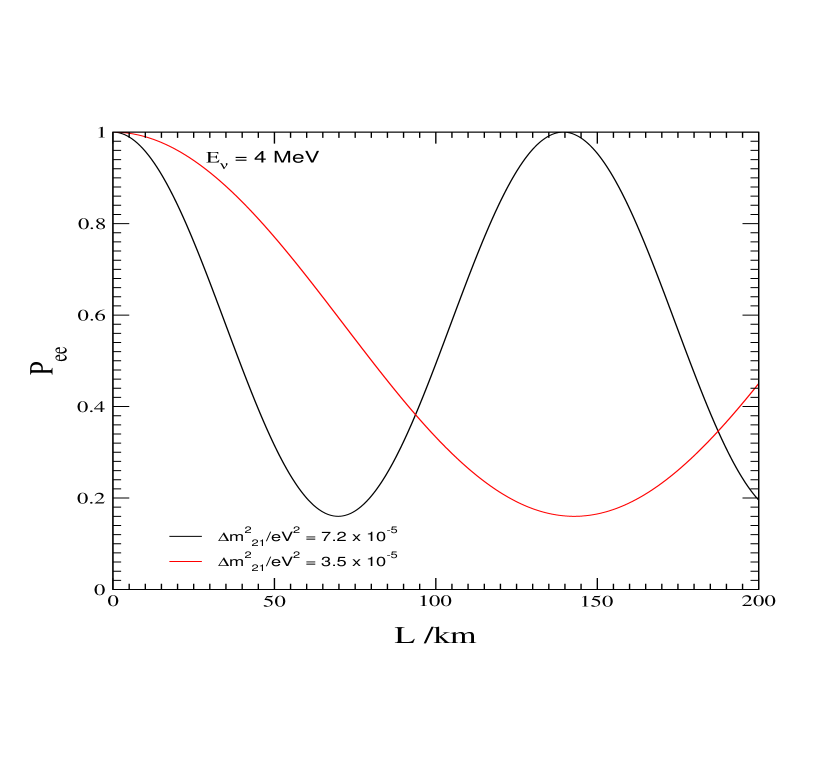
Figure 4: The probability vs distance for an average energy of 4 MeV for $\Delta m_{21}^{2}$  = $7.5\times 10^{-5}$eV² and 3.5 $\times 10^{-5}$ eV².

To trace the reason why the $\theta$ sensitivity is better at $3.5\times 10^{-5}$ eV² in figure 4 we plot the probability vs distance for energy fixed at 4 MeV. The figure shows that the average distance of $\sim$ 150 km of KamLAND corresponds to a maximum in the probability for $7.2\times 10^{-5}$ eV² while at $3.5\times 10^{-5}$ eV² corresponds to a minima.

The relevant survival probability for KamLAND is given by the vacuum oscillation expression

$$P_{ee}=1-\sum_{i}\sin^{2}2\mbox{$\theta_{\odot}$~{}}\sin^{2}\left(\frac{\mbox{$\Delta m_{21}^{2}$~{}}L_{i}}{4E}\right)$$ (2)

where $L_{i}$ stands for the different reactor distances and one needs to do an averaging over these. Three limits can be distinguished
$\bullet$ $\sin^{2}(\mbox{$\Delta m_{21}^{2}$~{}}L/4E)=0$ we get a Survival Probability MAXimum (SPMAX)
$\bullet$ $\sin^{2}(\mbox{$\Delta m_{21}^{2}$~{}}L/4E)=1$ we get a Survival Probability MINimum (SPMIN)
$\bullet$ $\sin^{2}(\mbox{$\Delta m_{21}^{2}$~{}}L/4E)=1/2$ we get averaged oscillation

In the LMA region the solar ${}^{8}{B}$ neutrinos undergo adiabatic MSW transition and the survival probability can be approximated as

$$P_{ee}({\mbox{${}^{8}{B}~{}$}})\approx\sin^{2}\mbox{$\theta_{\odot}$~{}}$$ (3)

Whereas the low energy $pp$ neutrinos do not undergo any MSW resonance and the survival probability is just the averaged oscillation probability in vacuum.

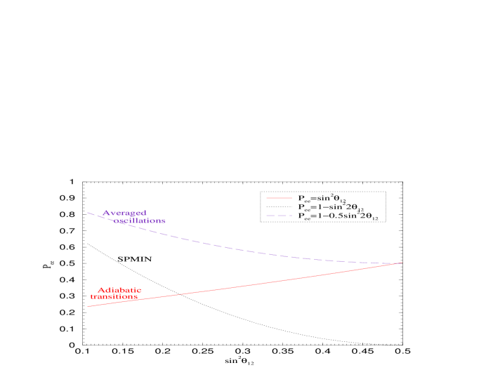
Figure 5: The survival probability $P_{ee}$ as a function $\sin^{2}\theta_{12}$.

In figure 5 we plot the $\theta$ dependence of the adiabatic MSW probability as well as the probability for the SPMIN and averaged oscillation case [11]. The figure shows that for large mixing angles close to maximal, the adiabatic case has the maximum sensitivity. For mixing angles not too close to maximal ($\sin^{2}\theta_{\odot}<0.38$) , the $P_{ee}$ for the SPMIN case has the sharpest dependence on the mixing angle and the $\theta_{\odot}$ sensitivity is maximum. Since the 99% C.L. allowed values of $\theta_{\odot}$ is within the range $0.22<\sin^{2}\mbox{$\theta_{\odot}$~{}}<0.44$, SPMIN seems most promising for constraining $\theta_{12}$. On the other hand at SPMAX the oscillatory term goes to zero and the $\theta_{12}$ sensitivity gets smothered. Since in the statistically significant region the KamLAND probability corresponds to an SPMAX for he best-fit value of $7.2\times 10^{-5}$ eV² the $\theta$ sensitivity of KamLAND is not as good as its $\Delta m_{21}^{2}$  sensitivity. For this value of $\Delta m_{21}^{2}$ the SPMIN comes at 70 km.

5 A dedicated reactor experiment for $\sin^{2}\theta_{\odot}$

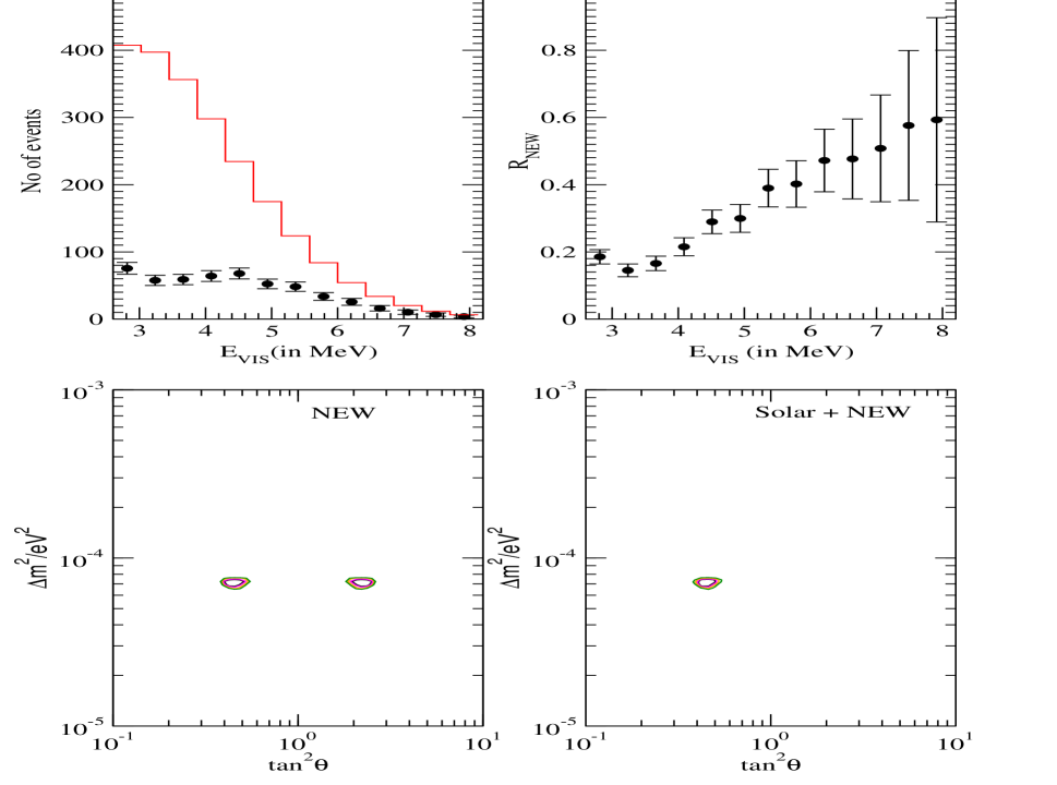
Figure 6: The spectrum and allowed regions for a new reactor experiment with a source detector distance of 70 km

We show in Figure 6 the constraints on the mass and mixing parameters obtained using a ”new” dedicated reactor experiment whose baseline is tuned to an oscillation SPMIN [11]. We use the antineutrino flux from a reactor a la Kashiwazaki nuclear reactor in Japan with a power of about 25 GWatt. We assume a 80% efficiency for the reactor output and simulate the 3 kTy data at the low-LMA best-fit for a KamLAND like detector placed at 70 km from the reactor source and which has systematic errors of only 2%. The top-left panel of the Figure 6 shows the simulated spectrum data. The histogram shows the expected spectrum for no oscillations. $E_{vis}$ is the “visible” energy of the scattered electrons. The top-right panel gives the ratio of the simulated oscillations to the no oscillation numbers. The sharp minima around $3-4$ MeV is clearly visible. The bottom-left panel gives the C.L. allowed areas obtained from this new reactor experiment data alone. With 3 kTy statistics we find a marked improvement in the $\theta_{\odot}$ bound with the 99% range $0.39<\tan^{2}\mbox{$\theta_{\odot}$~{}}<0.52$ giving a spread of 14% . The “dark side” solution appearing in the left lower panel because of the $\mbox{$\theta_{\odot}$~{}}-(\pi/2-\mbox{$\theta_{\odot}$~{}})$ ambiguity in the vacuum oscillations probability is ruled out in the right lower panel by the solar neutrino data. Recently sites of reactor neutrino experiments with a source-reactor distance of 70 km has been discussed in [12]. Also in Japan a new reactor complex SHIKA-2 at $\sim$ 88 km (close to SPMIN) will start in 2006 (See however [13]).

6 Other future experiments

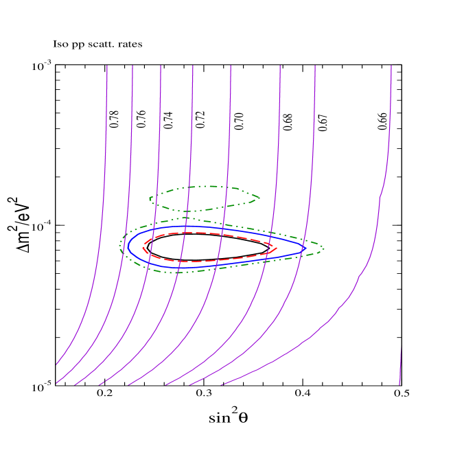
Figure 7: The isorates for a $pp$ scattering experiment.

In Figure 7 we show the lines of constant rate/SSM predicted in a generic LowNu electron scattering experiment sensitive to $pp$ neutrinos [14]. At these low energies neutrinos the survival probability in the LMA zone is $\approx 1-\frac{1}{2}\sin^{2}2\theta$ and has almost no sensitivity to $\Delta m_{21}^{2}$. But the $\sin^{2}\theta_{\odot}$ sensitivity is quite good and thus these experiments may have a fair chance to pin down the value of the mixing angle $\theta_{12}$, if they can keep the errors low.

7 Conclusions

The KamLAND experiment has not only confirmed the LMA solution to the solar neutrino problem it has narrowed down the allowed range of $\Delta m^{2}_{\odot}$  considerably owing to its sensitivity to the spectral distortion driven by this parameter. However the $\theta_{\odot}$  sensitivity of KamLAND is not as good. Baseline is important to identify which parameters would be best determined. We discuss that a SPMIN in the vacuum oscillation probability is important for the determination of the mixing angle. For the current best-fit $\Delta m^{2}_{\odot}$  in the low-LMA region SPMIN comes at a distance of 70 km . We propose a dedicated 70 km baseline reactor experiment to measure $\theta_{\odot}$  down to $\sim 10\%$ accuracy. LowNU experiments could be important for precise determination of $\theta_{\odot}$  if the experimental errors are low.

This talk is based on the work [11]. The updated analysis including the SNO salt results were done in collaboration with S.T.Petcov and D.P. Roy and the authors would like to acknowledge them. This work was supported in part by the Italian MIUR and INFN under ‘Fisica Astroparticellare” (S.C.).

References

- [1] Q. R. Ahmad et al. [SNO Collaboration], Phys. Rev. Lett. 89, 011301 (2002) [arXiv:nucl-ex/0204008]; Phys. Rev. Lett. 89, 011302 (2002) [arXiv:nucl-ex/0204009].
- [2] A. Bandyopadhyay, S. Choubey, S. Goswami and D. P. Roy, Phys. Lett. B 540, 14 (2002) [arXiv:hep-ph/0204286].
- [3] K. Eguchi et al. [KamLAND Collaboration], Phys. Rev. Lett. 90, 021802 (2003) [arXiv:hep-ex/0212021].
- [4] A. Bandyopadhyay, S. Choubey, R. Gandhi, S. Goswami and D. P. Roy, arXiv:hep-ph/0212146.
- [5] S. N. Ahmed et al. [SNO Collaboration], arXiv:nucl-ex/0309004.
- [6] A. Bandyopadhyay, S. Choubey, S. Goswami, S. T. Petcov and D. P. Roy, arXiv:hep-ph/0309174.
- [7] B. T. Cleveland et al., Astrophys. J. 496, 505 (1998); J. N. Abdurashitov et al. [SAGE Collaboration], arXiv:astro-ph/0204245; W. Hampel et al. [GALLEX Collaboration], Phys. Lett. B 447, 127 (1999); M. Altmann et al., (The GNO collaboration),Phys. Lett. B492,16 (2000); C.M. Cattadori, Nucl. Phys. B110, Proc. Suppl, 311 (2002).
- [8] S. Fukuda et al. [Super-Kamiokande Collaboration], Phys. Lett. B 539, 179 (2002) [arXiv:hep-ex/0205075].
- [9] S. Choubey, A. Bandyopadhyay, S. Goswami and D. P. Roy, arXiv:hep-ph/0209222.
- [10] A. Bandyopadhyay, S. Choubey, R. Gandhi, S. Goswami and D. P. Roy, arXiv:hep-ph/0211266.
- [11] A. Bandyopadhyay, S. Choubey and S. Goswami, Phys. Rev. D 67, 113011 (2003) [arXiv:hep-ph/0302243].
- [12] C. Bouchiat, arXiv:hep-ph/0304253.
- [13] A. Bandyopadhyay, S. Choubey, S. Goswami and S. T. Petcov, arXiv:hep-ph/0309236.
- [14] For a discussion on LowNU experiments see e.g. S. Schönert, talk at Neutrino 2002, Munich, Germany, (http://neutrino2002.ph.tum.de).
- [15] S. Choubey, S. T. Petcov and M. Piai, arXiv:hep-ph/0306017.