Diffractive photon dissociation in the saturation regime
from the Good and Walker picture

Abstract

Combining the QCD dipole model with the Good and Walker picture, we formulate diffractive dissociation of a photon of virtuality $Q^{2}$ off a hadronic target, in the kinematical regime in which $Q$ is close to the saturation scale and much smaller than the invariant mass of the diffracted system. We show how the obtained formula compares to the HERA data and discuss what can be learnt from such a phenomenology. In particular, we argue that diffractive observables in these kinematics provide useful pieces of information on the saturation regime of QCD.

I Introduction

Hard diffraction has triggered a wide interest since its discovery in high energy virtual photon-proton scattering at HERA Derrick:1993xh . It has been a major theoretical challenge to understand the observed large rate of diffractive events within QCD, especially for large virtualities $Q^{2}$ of the photon (for a review, see Ref. Hebecker:1999ej ). Among the attempts to describe hard diffraction, the dipole picture of QCD Nikolaev:1991ja ; Mueller:1994rr including unitarization corrections Golec-Biernat:1998js has proved particularly successful and natural in embedding both inclusive and diffractive observables in the same conceptual framework Nikolaev:1991ja ; Nikolaev:1992et ; Mueller:1994jq ; Bialas:1998vt .

There are two distinct processes contributing to diffractive final states. A first one consists in the photon splitting in a $q\bar{q}$ pair, which scatters elastically off the target without any further radiation. The final state has typically a low invariant mass $M_{X}$, of the order of the virtuality of the photon. A second contribution is due to the $q\bar{q}$ pair interacting through higher Fock state fluctuations, for example $q\bar{q}g$, which go instead to a large-mass final state $M_{X}\gg Q$. The latter process is called diffractive dissociation of the photon. As there is a clear kinematical separation between the two processes, it makes sense to analyse these contributions separately. The present paper deals with the second one, i.e. diffractive dissociation.

To select this particular process one needs a large hierarchy between the mass of the diffractive final state and the virtuality of the photon. This means in practice that one is forced to relatively low virtuality scales $Q^{2}\!\leq\!1\ \mbox{GeV}^{2}$, because of limited total center-of-mass energy available in the experiments. However, the process can still be computable in perturbative QCD provided that the energy is high enough to push the intrinsic $k_{\bot}$ of the partons inside the proton to large values $k_{\bot}\!\sim\!Q_{s}\!\gg\!\Lambda_{\mbox{\footnotesize QCD}}$. This feature is a consequence of the saturation of parton densities Gribov:1981ac and is now well-understood within QCD Gribov:1981ac ; McLerran:1994ni ; Balitsky:1996ub . $Q_{s}$ is called the saturation scale, and is an increasing function of the rapidity of the proton.

The dipole picture is well-suited because color dipoles, which are two-body color neutral objets characterized by their longitudinal momentum, transverse size and impact parameter, are eigenstates of the QCD interaction at high energy. Both elastic scattering (and thus, from the optical theorem, the total cross section) and diffractive dissociation have a straightforward formulation in terms of dipoles. The latter is most simply obtained from the Good and Walker mechanism Good:1960ba ; Peschanski:1998cs .

Our interest in diffractive dissociation is triggered by the wealth of new data that are being taken in the relevant kinematical range at HERA. On the other hand, while some theoretical calculations are already available in the literature Kovchegov:2001ni ; Kovner:2001vi , to our knowledge there has been no phenomenological analysis of this particular kinematical domain within QCD saturation models. Ref. Golec-Biernat:1998js provides a model also for diffractive dissociation, but the approximations made there allowed only for high virtualities of the photon $Q\!\gg\!Q_{s}$, therefore the obtained formulae are unapplicable to the recent data at low $Q^{2}$.

In the following, we wish to clearly distinguish what is theoretically well under control and which are the model assumptions that have to be made to come to the description of the HERA data. In this spirit, we will start by providing a complete derivation for the idealized process of diffractive dissociation of a photon on a large nucleus, for which the saturation corrections can be implemented in an easier way. This will be done in Sec. II. Some analytical results are given in Sec. III. In Sec. IV, we turn to phenomenology and explain how we can adapt the obtained results to photon-proton reactions at HERA. We compare our predictions to recently analyzed data. Our conclusions are drawn in Sec. V.

II Diffractive dissociation of a virtual photon on a large nucleus

In this section, we compute the cross section for diffractive production of a hadronic system of large mass $M_{X}$ in a highly energetic photon-nucleus collision. We limit ourselves to diffracted systems which have the following partonic content: $q\bar{q}$ or $q\bar{q}g$. Higher Fock states are indeed not needed for large but still moderate values of $M_{X}$. The target is a large nucleus because, as will be discussed, complete and numerically manageable results can be obtained strictly speaking only in this idealized framework. We will also stick to the large-$N_{c}$ limit, and to the semi-classical approximation implied by the high energy kinematics.

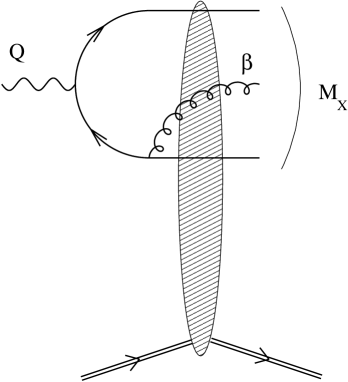
Figure 1: One of the relevant graphs contributing to diffractive dissociation of the photon. The blob denotes the elastic double dipole-proton cross section.

II.1 High energy kinematics and dipoles

We go to a frame (the so-called dipole frame Mueller:2001fv ) in which the photon and the nucleus have respective 4-momenta $q^{\mu}=(q^{+},-Q^{2}/(2q^{+}),0^{\bot})$ and $p^{\mu}=(0,p^{-},0^{\bot})$. The total squared center-of-mass energy is given by $s=2q^{+}p^{-}\!-\!Q^{2}$. Through an appropriate boost along the collision axis, the value of $q^{+}$ is chosen such that the whole diffracted partonic state $|q\bar{q}\rangle$ or $|q\bar{q}g\rangle$ is viewed as a quantum fluctuation of the photon which subsequently scatters off the nucleus. The nucleus contains all partonic fluctuations due to the remaining energy evolution as part of its wave function at the time of the interaction. This is possible in a frame in which the rapidity of the slowest final-state particle is close to zero. Of course, the observables will not depend on the frame, but our choice provides a physical picture which is particularly adapted to the study of unitarization effects. The event is diffractive if the nucleus does not break up, which requires the scattering to proceed through the exchange of a color-neutral object.

It was proven McLerran:1994ni ; Balitsky:1996ub (for a review, see Iancu:2003xm ) that in the dipole frame, the mean transverse momentum of the partons in the nucleus is shifted from $\Lambda_{\mbox{\footnotesize QCD}}$ to a scale $Q_{s}$ (the so-called saturation scale) which increases with the rapidity of the nucleus, due to multiple scatterings and saturation of the parton densities Gribov:1981ac ; Mueller:1990st that occur to preserve the unitarity of the scattering matrix. If the energy is large, then the saturation scale can become high enough $Q_{s}\gg\Lambda_{\mbox{\footnotesize QCD}}$ to justify perturbative calculations for the diffracted partonic system, even if the transverse momenta at the level of the photon, initially of order $Q$, are not large.

In the dipole frame, the time sequence of the interaction is the following: the photon couples to a $q\bar{q}$ pair, which then radiates (or not) a gluon before the whole system scatters off the nucleus through the exchange of a color-neutral object. The leading terms at high center-of-mass energy $s$ come about when the ordering in time is strict, i.e. when the intermediate $q\bar{q}$ can be considered an almost on-shell onium state. The following factorization then holds:

$$\frac{d\sigma_{\mbox{\footnotesize diff}}^{\gamma}}{d^{2}b}=\int d^{2}r\int_{0}^{1}dz\left(|\psi_{T}^{\gamma}(r,z;Q)|^{2}+|\psi_{L}^{\gamma}(r,z;Q)|^{2}\right)\frac{d\sigma_{\mbox{\footnotesize diff}}}{d^{2}b}\ ,$$ (1)

where $r$ is the transverse size of the $q\bar{q}$ pair, $b$ its impact parameter, and $z$ is the longitudinal momentum fraction of the antiquark. $d\sigma_{\mbox{\footnotesize diff}}/d^{2}b$ is the onium-nucleus diffractive cross section. The photon wave functions $\psi^{\gamma}_{T}$, $\psi^{\gamma}_{L}$ on a $q\bar{q}$ pair are given by Bjorken:1971ah

$$\begin{split}|\psi^{\gamma}_{T}(r,z;Q)|^{2}&=\frac{3\alpha_{em}}{2\pi^{2}}\sum_{f}e_{f}^{2}\left((z^{2}+(1-z)^{2})\varepsilon_{f}^{2}K_{1}^{2}(\varepsilon_{f}|r|)+m_{f}^{2}K_{0}^{2}(\varepsilon_{f}|r|)\right)\\ |\psi^{\gamma}_{L}(r,z;Q)|^{2}&=\frac{3\alpha_{em}}{2\pi^{2}}\sum_{f}e_{f}^{2}4Q^{2}z^{2}(1-z)^{2}K_{0}^{2}(\varepsilon_{f}|r|)\end{split}$$ (2)

for a transversely and longitudinally polarized photon respectively. Here we sum over both polarizations, but in practice in the kinematical domain of interest ($Q^{2}$ not too large), only the transverse component will be relevant. In the previous formula, $m_{f}$ is the mass of quark $f$ and

$$\varepsilon_{f}=\sqrt{z(1-z)Q^{2}+m_{f}^{2}}\ .$$ (3)

Thanks to the factorization (1), it will be enough to compute the cross section $d\sigma_{\mbox{\footnotesize diff}}/d^{2}b$ for diffractive dissociation of an onium. Using that formula, we will be able to relate it in fine in a straightforward way to the deep-inelastic scattering observables.

Recalling that $q^{+}$ is the lightcone momentum of the incident photon, the 4-momenta of the partons in its wave function read

$$\mbox{quark:}\ (z_{q}q^{+},\frac{k_{q}^{2}}{2z_{q}q^{+}},k_{q})\ ,\ \mbox{antiquark:}\ (z_{\bar{q}}q^{+},\frac{k_{\bar{q}}^{2}}{2z_{\bar{q}}q^{+}},k_{\bar{q}})\ ,\ \mbox{gluon:}\ (z_{g}q^{+},\frac{k_{g}^{2}}{2z_{g}q^{+}},k_{g})$$ (4)

where $z_{q}+z_{\bar{q}}+z_{g}=1$ and $k_{q}+k_{\bar{q}}+k_{g}=0$ from conservation of the 3-momentum. The transverse momenta $k_{q}$, $k_{\bar{q}}$ and $k_{g}$ are of the order of the external mass and/or virtuality scales which we assume all of the same magnitude $Q\gg\Lambda_{\mbox{\footnotesize QCD}}$. We require furthermore the diffracted system to have a large mass in the sense $M_{X}\gg Q$. Then the squared invariant mass of this partonic system reads

$$M_{X}^{2}=Q^{2}\left(\frac{1}{z_{q}}+\frac{1}{z_{\bar{q}}}+\frac{1}{z_{g}}\right)$$ (5)

and gets large if either $z_{q}$, $z_{\bar{q}}$ or $z_{g}$ are small. Due to the infrared singularity of QCD, $z_{g}$ is very small in a typical configuration, in which case $M_{X}^{2}=Q^{2}/z_{g}$. This configuration with strong ordering of longitudinal momenta $z_{g}\ll z_{q},z_{\bar{q}}$ is the dominant contribution in the kinematical regime of interest. Thus the mass of the diffractive final state is directly related to the longitudinal momentum fraction of the photon carried by the gluon.

Let us now introduce some more kinematics. The difference between the rapidity of the onium and the rapidity of the slowest particle in the final state is denoted by $y_{X}$. If $\beta$ is the fraction of momentum of this particle with respect to the initial-state onium, then it is easy to see that $y_{X}=\log(1/\beta)$. One also sees that $\beta=z_{g}$ for a $|q\bar{q}g\rangle$ final state. The total rapidity difference between the photon and the nucleus is denoted by $y=\log(1/x_{Bj})$, where $x_{Bj}$ is the Bjorken variable. Then one introduces the rapidity gap variable $y_{\mathbb{P}}=y-y_{X}$ and similarly to $\beta$, the variable $x_{\mathbb{P}}$ such that $y_{\mathbb{P}}=\log(1/x_{\mathbb{P}})$. The relationship between these variables and the kinematics of the event reads

$$\beta=\frac{Q^{2}}{Q^{2}+M_{X}^{2}}\ ,\ \ \ x_{Bj}=\frac{Q^{2}}{Q^{2}+s}\ ,\ \ \ x_{\mathbb{P}}=\frac{x_{Bj}}{\beta}=\frac{Q^{2}+M_{X}^{2}}{Q^{2}+s}\ .$$ (6)

The quantity which is measured and which will be computed is the differential cross section $d\sigma_{\mbox{\footnotesize diff}}^{\gamma}/dM_{X}$ or equivalently $d\sigma_{\mbox{\footnotesize diff}}^{\gamma}/d\log(1/\beta)$. They are related by a simple kinematical factor:

$$\frac{d\sigma_{\mbox{\footnotesize diff}}^{\gamma}}{dM_{X}}=\frac{2M_{X}}{Q^{2}+M_{X}^{2}}\frac{d\sigma_{\mbox{\footnotesize diff}}^{\gamma}}{d\log(1/\beta)}\underset{M_{X}^{2}\gg Q^{2}}{=}\frac{2}{M_{X}}\frac{d\sigma_{\mbox{\footnotesize diff}}^{\gamma}}{d\log(1/\beta)}\ .$$ (7)

The calculation of the cross section for diffractive production of a gluon in onium-nucleus scattering will proceed in two steps. In the next subsection we compute the elastic scattering amplitude for the onium on the nucleus up to order ${\cal O}(\alpha_{s})$. Then we will deduce the diffractive cross section from the Good and Walker formula and with the help of the elastic amplitude.

II.2 Elastic amplitude at next-to-leading order

We only keep the leading terms in a $1/N_{c}$ expansion. Then, as well-known, the partonic content of a color neutral object can be represented as a set of dipoles (see Fig. 2).

$$\begin{array}[]{ccc}\mbox{\psfig{width=113.81102pt}}&\phantom{ungrandespace}&\mbox{\psfig{width=113.81102pt}}\\ \\ \phantom{espace}\mbox{(a)}&&\phantom{espace}\mbox{ (b)}\end{array}$$

Figure 2: (a) The $q\bar{q}g$ Fock state decomposition of the photon. (b) The same in the large-$N_{c}$ limit.

We denote by $x_{i}$ (a 2-dimensional vector) the transverse position of the dipole constituent $i$ with respect to the center of the target, $x_{ij}=x_{i}-x_{j}$, and $z_{i}$ is the fraction of longitudinal momentum carried by constituent $i$. The normalization of a generic dipole state is given by the orthogonality condition

$$\langle x,b,z|x^{\prime},b^{\prime},z^{\prime}\rangle=\delta^{2}(x-x^{\prime})\delta^{2}(b-b^{\prime})\delta(z-z^{\prime})$$ (8)

for two dipoles of respective sizes $x$, $x^{\prime}$ and center-of-mass coordinate vectors $b$, $b^{\prime}$. In the following, unless it might hamper understanding, one does not keep track of the $z$-variables in order to simplify the notations.

The physical dipole state $|x_{01},b\rangle_{\mbox{\footnotesize phys}}$ in the initial state of the experiment is dressed with all possible fluctuations. Its expansion in terms of bare Fock states reads

$$|x_{01},b\rangle_{\mbox{\footnotesize phys}}=\sqrt{Z(x_{01})}|x_{01},b\rangle+\int d^{2}x_{2}dz_{2}\,\psi(x_{02},x_{12},z_{2})|x_{02},x_{12},b\rangle+\cdots$$ (9)

where $\psi(x_{02},x_{12},z_{2})$ is the probability amplitude that the dipole $x_{01}$ split in two dipoles of respective sizes $x_{02}$ and $x_{12}$, which corresponds to a 1-gluon fluctuation of the initial onium. The gluon has longitudinal momentum fraction $z_{2}$. Note that $|\psi|^{2}$ is of order $\alpha_{s}$, and the higher Fock states not written are at least of order $\alpha_{s}^{2}$: this remark provides the systematics for this Fock-state expansion, seen as a perturbative expansion in the parameter $\alpha_{s}$. This expansion is relevant since $\alpha_{s}$ is small because it runs with a scale between $Q_{s}$ and $Q$, which we have both assumed much larger than $\Lambda_{\mbox{\footnotesize QCD}}$. Also, note that the 2-dipole state is not renormalized to this order, but would get renormalized from higher orders.

The quantity that will appear in the calculation of observables is the squared wave function, summed over the polarizations and colors of the final-state gluon, whose expression can be found in Mueller:1994rr :

$$\phi(x_{02},x_{12},z_{2})\equiv\sum_{\mbox{\footnotesize polarization \& color}}|\psi(x_{02},x_{12},z_{2})|^{2}=\frac{\alpha_{s}N_{c}}{2\pi^{2}}\frac{1}{z_{2}}\frac{x_{01}^{2}}{x_{02}^{2}x_{12}^{2}}\ .$$ (10)

From the unitarity condition (8) applied to the physical state $|x_{01},b\rangle_{\mbox{\footnotesize phys}}$ in (9), one can compute the renormalization constant $Z$

$$Z(x_{01})=1-\int_{\rho^{2}}d^{2}x_{2}\int_{\beta}^{1}dz_{2}\,\phi(x_{02},x_{12},z_{2})\ ,$$ (11)

where $\rho$ cuts off the ultraviolet divergences and $\beta$ the infrared ones. In practice, as it should be $\rho$ disappears from physical quantities, and $\beta$ is fixed by the kinematical limit. Note that $Z$ represents physically the probability that the initial onium does not radiate any gluon.

Let us denote by $\mathbb{S}$ the scattering matrix of the onium on the nucleus. Color dipoles form an orthogonal basis of the interaction eigenstates at high energy, thus the ${\mathbb{S}}$-matrix element between two dipole states reads

$$\langle x,b|{\mathbb{S}}|x^{\prime},b^{\prime}\rangle=\delta^{2}(x-x^{\prime})\delta^{2}(b-b^{\prime})S(x,b,x_{\mathbb{P}})\ .$$ (12)

The quantity $|S(x,b,x_{\mathbb{P}})|^{2}$ is the probability that a dipole of size $x$ at impact parameter $b$ does not interact with the target. The $x_{\mathbb{P}}$-dependence of this quantity reflects the high energy evolution of the target.

The ${\mathbb{S}}$-matrix element between two double dipole states reads

$$\langle x_{02},x_{12},b|{\mathbb{S}}|x^{\prime}_{02},x^{\prime}_{12},b^{\prime}\rangle=\delta^{2}(x_{02}-x^{\prime}_{02})\delta^{2}(x_{12}-x^{\prime}_{12})\delta^{2}(b-b^{\prime})S(x_{02},x_{12},b,x_{\mathbb{P}})\ .$$ (13)

The notation is the following: $S(x_{02},x_{12},b,x_{\mathbb{P}})$ is the elastic diffusion matrix element for states formed of two adjacent dipoles of respective sizes $x_{02}$ and $x_{12}$, and $b=(x_{0}+x_{1})/2$. The quantity $|S(x_{02},x_{12},b,x_{\mathbb{P}})|^{2}$ is the probability that neither $x_{02}$ nor $x_{12}$ interact, which under the assumption that the dipoles interact independently is the product of the probabilities that $x_{02}$ and $x_{12}$ do not interact, $|S(x_{02},b-x_{12}/2,x_{\mathbb{P}})|^{2}|S(x_{12},b-x_{02}/2,x_{\mathbb{P}})|^{2}$. The latter assumption is justified when the target is a large nucleus, since nucleons are color-neutral and independent. As furthermore ${\mathbb{S}}$ is known to be real at high energy, one can get rid of the squared modulus and one gets

$$S(x_{02},x_{12},b,x_{\mathbb{P}})=S(x_{02},b-x_{12}/2,x_{\mathbb{P}})S(x_{12},b-x_{02}/2,x_{\mathbb{P}})\ .$$ (14)

Next one expresses the scattering matrix for the physical dipole $|x_{01},b\rangle_{\mbox{\footnotesize phys}}$ as

$${}_{\mbox{\footnotesize phys}}\langle x_{01},b|{\mathbb{S}}|x^{\prime}_{01},b^{\prime}\rangle_{\mbox{\footnotesize phys}}=Z\langle x_{01},b|{\mathbb{S}}|x^{\prime}_{01},b^{\prime}\rangle\\ +\int_{\rho^{2}}d^{2}x_{2}d^{2}x^{\prime}_{2}\int_{\beta}^{1}dz_{2}dz_{2}^{\prime}\,\psi^{*}(x_{02},x_{12},z_{2})\psi(x^{\prime}_{02},x^{\prime}_{12},z^{\prime}_{2})\,\langle x_{02},x_{12},b|{\mathbb{S}}|x^{\prime}_{02},x^{\prime}_{12},b^{\prime}\rangle\ .$$ (15)

Using Eqs. (11,12,14), and performing the integration over $x^{\prime}_{01}$ and $b^{\prime}$, one gets for the diffusion amplitude

$${\cal T}(x_{01},b,\beta,x_{\mathbb{P}})=T(x_{01},b,x_{\mathbb{P}})\\ +\frac{\alpha_{s}N_{c}}{2\pi^{2}}\int_{\beta}^{1}\frac{dz_{2}}{z_{2}}\int d^{2}x_{2}\,\frac{x_{01}^{2}}{x_{02}^{2}x_{12}^{2}}\left(S(x_{01},b,x_{\mathbb{P}})-S(x_{02},b\!-\!x_{12}/2,x_{\mathbb{P}})S(x_{12},b\!-\!x_{02}/2,x_{\mathbb{P}})\right)\ ,$$ (16)

where $T$ stands for the matrix elements of ${\mathbb{T}}=1-{\mathbb{S}}$ between bare states, and ${\cal T}$ are its matrix elements betweeen dressed states. The UV cutoff has been removed because when either $x_{02}$ or $x_{12}$ tends to 0, then because of color transparency, the factor built from the ${\mathbb{S}}$-matrix elements vanishes like $x^{2}_{02}$ (resp. $x^{2}_{12}$), and thus the integral over $x_{2}$ is finite. The first term in Eq. (16) is the Born term, the second one is the ${\cal O}(\alpha_{s})$ correction to it. Physically, $\cal T$ is the amplitude for inclusive production of a forward gluon having longitudinal momentum larger than $\beta q^{+}$, when the total available rapidity is $y=\log(1/\beta x_{\mathbb{P}})$.

At this point, it is interesting to note that the procedure described above can be iterated to get the Balitsky-Kovchegov (BK) equation Balitsky:1996ub . The latter gives the evolution of the dipole-nucleus ${\mathbb{S}}$-matrix element for a dressed dipole $\hat{S}(x_{01},b,\beta,x_{\mathbb{P}})$ when the total rapidity $y\!=\!\log(1/x_{Bj})\!=\!\log(1/\beta x_{\mathbb{P}})$ increases. Starting from the scattering of a bare onium at $\beta\!=\!1$, Eq. (16) gives the evolution of the amplitude ${\cal T}=1-\hat{S}(x_{01},b,\beta,x_{\mathbb{P}})$ as one decreases $\beta$, i.e. as one gives a small boost to the onium while the rapidity of the target is kept fixed. The change of the amplitude comes from the fact that the onium can now be found with an extra gluon in its wave function: in the large $N_{c}$ limit, this means that the onium has a probability to be formed of two adjacent dipoles. Then under the assumption that the dipoles interact independently, for example with different nucleons of a large nucleus, this procedure can be iterated by simply replacing the ${\mathbb{S}}$-matrix element for bare dipoles in the r.h.s. of Eq. (16) (for which $\beta\!=\!1$) by the ${\mathbb{S}}$-matrix element for the scattering of dressed dipoles at total rapidity $\log(1/z_{2}x_{\mathbb{P}})<\log(1/\beta x_{\mathbb{P}})$, which reads $\hat{S}(x_{01},b,z_{2},x_{\mathbb{P}})$. One gets the following integral equation:

$$\hat{S}(x_{01},b,\beta,x_{\mathbb{P}})=S(x_{01},b,x_{\mathbb{P}})\\ +\frac{\alpha_{s}N_{c}}{2\pi^{2}}\int_{\beta}^{1}\frac{dz_{2}}{z_{2}}\int d^{2}x_{2}\,\frac{x_{01}^{2}}{x_{02}^{2}x_{12}^{2}}\left(\hat{S}(x_{02},b-x_{12}/2,z_{2},x_{\mathbb{P}})\hat{S}(x_{12},b-x_{02}/2,z_{2},x_{\mathbb{P}})-\hat{S}(x_{01},b,z_{2},x_{\mathbb{P}})\right)\ .$$ (17)

One now takes the derivative of both sides with respect to $\log(1/\beta)$. As we keep $x_{\mathbb{P}}$ fixed, this is equivalent to taking the derivative with respect to the total rapidity $\log(1/x_{Bj})$ and one gets

$$\frac{\partial{\hat{S}}(x_{01},b,x_{Bj})}{\partial\log(1/x_{Bj})}=\frac{\alpha_{s}N_{c}}{2\pi^{2}}\int d^{2}x_{2}\,\frac{x_{01}^{2}}{x_{02}^{2}x_{12}^{2}}\left(\hat{S}(x_{02},b-x_{12}/2,x_{Bj})\hat{S}(x_{12},b-x_{02}/2,x_{Bj})-\hat{S}(x_{01},b,x_{Bj})\right)\ ,$$ (18)

which is indeed the BK equation Balitsky:1996ub (see Ref. Mueller:2001fv for a derivation closely related to ours). This equation resums the so-called “fan diagrams”.

Coming back to Eq. (16) for ${\cal T}$, the total cross section stems from the optical theorem, and the elastic cross section is the squared amplitude ${\cal T}$:

$$\frac{d\sigma_{\mbox{\footnotesize tot}}}{d^{2}b}=2{\cal T}(x_{01},b)\ \ \ \mbox{and}\ \ \ \frac{d\sigma_{\mbox{\footnotesize el}}}{d^{2}b}=|{\cal T}(x_{01},b)|^{2}\ .$$ (19)

II.3 Diffraction from the Good and Walker picture

An elegant and most straightforward formulation of diffractive dissociation is obtained by using the Good and Walker Good:1960ba picture (see also Miettinen:1978jb and Peschanski:1998cs ), according to which inelastic diffraction is proportional to the dispersion in cross sections for the diagonal channels of the scattering. The reason why we are relying on such a picture, developed in the context of early hadronic physics Good:1960ba and subsequently extended to the parton model Miettinen:1978jb , is that the dipoles form precisely a complete set of eigenstates of the QCD interaction at high energy. The cross section for diffractive dissociation reads in this picture

$$\frac{d\sigma_{\mbox{\footnotesize diff}}}{d^{2}b}=\int d^{2}x^{\prime}_{01}d^{2}b^{\prime}\sum_{X}{}_{\mbox{\footnotesize phys}}\langle x_{01},b|{\mathbb{T}}^{\dagger}|X\rangle\langle X|{\mathbb{T}}|x^{\prime}_{01},b^{\prime}\rangle_{\mbox{\footnotesize phys}}-\left|\int d^{2}x^{\prime}_{01}d^{2}b^{\prime}{}_{\mbox{\footnotesize phys}}\langle x_{01},b|{\mathbb{T}}|x^{\prime}_{01},b^{\prime}\rangle_{\mbox{\footnotesize phys}}\right|^{2}\ ,$$ (20)

where $X$ is any dipole final state, and the sum over $X$ also contains an integration over phase space of the type $\int\prod d^{2}x_{a}dz_{a}$. One denotes by (I) and (II) the (positive) terms appearing in this equation.

The second term is the easiest to compute since it is simply ${d\sigma_{\mbox{\footnotesize el}}}/{d^{2}b}$ (see formula (19)). Keeping only the terms relevant at order ${\cal O}(\alpha_{s})$, one gets

$$\mbox{(II)}=\frac{d\sigma_{\mbox{\footnotesize el}}}{d^{2}b}=T^{2}(x_{01},b,x_{\mathbb{P}})+\frac{\alpha_{s}N_{c}}{\pi^{2}}\int_{\beta}^{1}\frac{dz_{2}}{z_{2}}\int d^{2}x_{2}\frac{x_{01}^{2}}{x_{02}^{2}x_{12}^{2}}(1-S(x_{01}))(S(x_{01})-S(x_{02})S(x_{12}))\ .$$ (21)

Coming back to the first term in Eq. (20), the sum over $X$ is restricted to single $|x_{ab};b\rangle$ and double $|x_{ac},x_{bc};b\rangle$ dipole states, since we limit ourselves to the order ${\cal O}(\alpha_{s})$ of perturbation theory. At high energy the interaction with the target cannot change the number of dipoles in the wave function, the first term thus gives

$$\mbox{(I)}=\int d^{2}x^{\prime}_{01}d^{2}b^{\prime}\bigg{\{}Z(x_{01})\int d^{2}x_{ab}d^{2}b^{\prime\prime}\langle x_{01},b|{\mathbb{T}}^{\dagger}|x_{ab},b^{\prime\prime}\rangle\langle x_{ab},b^{\prime\prime}|{\mathbb{T}}|x^{\prime}_{01},b^{\prime}\rangle\\ +\int d^{2}x_{2}d^{2}x^{\prime}_{2}d^{2}x_{ac}d^{2}x_{bc}d^{2}b^{\prime\prime}\psi^{\dagger}(x_{02},x_{12})\psi(x^{\prime}_{02},x^{\prime}_{12})\\ \times\langle x_{02},x_{12},b|{\mathbb{T}}^{\dagger}|x_{ac},x_{bc},b^{\prime\prime}\rangle\langle x_{ac},x_{bc},b^{\prime\prime}|{\mathbb{T}}|x^{\prime}_{02},x^{\prime}_{12},b^{\prime}\rangle\bigg{\}}\ .$$ (22)

Eq. (11) enables one to express $Z(x_{01})$ and Eqs. (13,14) to replace the matrix elements. Then one uses the $\delta$-functions coming in Eqs. (13,14) which are due to the fact that the dipoles are eigenstates of the interaction, to perform the integrations over $x^{\prime}_{01}$, $x^{\prime}_{2}$, $x_{ab}$, $x_{ac}$, $x_{bc}$, $b^{\prime}$, $b^{\prime\prime}$. One finds

$$\mbox{(I)}=T^{2}(x_{01})+\frac{\alpha_{s}N_{c}}{2\pi^{2}}\int_{\beta}^{1}\frac{dz_{2}}{z_{2}}\int d^{2}x_{2}\frac{x_{01}^{2}}{x_{02}^{2}x_{12}^{2}}\left\{(1-S(x_{02})S(x_{12}))^{2}-(1-S(x_{01}))^{2}\right\}\ .$$ (23)

Putting the two parts (I) and (II) together and taking the derivative with respect to $\log(1/\beta)$, one gets after some straightforward algebra

$$\frac{d\sigma_{\mbox{\footnotesize diff}}}{d^{2}b\,d\log(1/\beta)}=\frac{\alpha_{s}N_{c}}{2\pi^{2}}\int d^{2}x_{2}\frac{x_{01}^{2}}{x_{02}^{2}x_{12}^{2}}(S(x_{02},b-x_{12}/2,x_{\mathbb{P}})S(x_{12},b-x_{02}/2,x_{\mathbb{P}})-S(x_{01},b,x_{\mathbb{P}}))^{2}\ .$$ (24)

A few technical remarks are in order. Our result is identical to the one obtained in earlier derivations within different frameworks (semi-classical Kovchegov:2001ni , eikonal Kovner:2001vi ). It is also consistent, in the weak interaction limit in which $T=1-S\ll 1$, with previous calculations Nikolaev:1994th , and in particular with the computation of all Feynman diagrams contributing to the $q\bar{q}g$ final state Bartels:1999tn .

Diagrams with gluons emitted in the final state are not included in our calculation since the radiative corrections we have concern exclusively the wave-function: no final state interaction can be accounted for in our calculation. This class of diagrams contributes to the diffractive final state, but they cancel out if one does not measure the transverse momentum of the gluon (see Chen:1995pa ; Mueller:2001fv ). Note that we could not obtain more detailed properties of the final state within our derivation, but as demonstrated earlier, thanks to the selected kinematics we do not need them for our purpose.

Using the factorization (1) and the kinematical relation (7), one gets the cross section for diffractive dissociation of a virtual photon in the form

$$\frac{d\sigma_{\mbox{\footnotesize diff}}^{\gamma}}{dM_{X}}=\frac{\alpha_{s}N_{c}}{\pi^{2}}\frac{1}{M_{X}}\int d^{2}x_{01}\int_{0}^{1}dz\left(|\psi_{T}^{\gamma}(z,x_{01};Q)|^{2}+|\psi_{L}^{\gamma}(z,x_{01};Q)|^{2}\right)\\ \times\int d^{2}x_{2}\frac{x_{01}^{2}}{x_{02}^{2}x_{12}^{2}}\int d^{2}b\,(S(x_{02},b-x_{12}/2,x_{\mathbb{P}})S(x_{12},b-x_{02}/2,x_{\mathbb{P}})-S(x_{01},b,x_{\mathbb{P}}))^{2}\ .$$ (25)

Equation (25) has to be evaluated numerically for a general dipole-nucleus ${\mathbb{S}}$-matrix, but there are two interesting limits that can be studied analytically, namely $Q^{2}\gg Q_{s}^{2}$ and $Q^{2}\ll Q_{s}^{2}$. This is done in the next section.

III Analytical insight

We will need a few general properties of the ${\mathbb{S}}$-matrix element:

$$S(r) \underset{|r|\gg 1/Q_{s}}{\ll}1$$ (black disk limit) (26)

$$1-S(r) \underset{|r|\ll 1/Q_{s}}{\sim}Q_{s}^{2}r^{2} \text{(color transparency)}\ .$$ (27)

Let us also recall that this theoretical study assumes enough center-of-mass energy so that $Q_{s}^{2}\gg\Lambda_{\mbox{\footnotesize QCD}}^{2}$ in the dipole frame. This also means that the dipole sizes entering formula (24), of order $1/Q_{s}$, are always smaller than the typical scale $1/\Lambda_{\mbox{\footnotesize QCD}}$ of the variations of the ${\mathbb{S}}$-matrix as a function of the impact parameter. Thus $S(x_{02},b-x_{12}/2)\simeq S(x_{02},b)$ and $S(x_{12},b-x_{02}/2)\simeq S(x_{12},b)$. We will not have to take care anymore of the $b$-dependence in the ${\mathbb{S}}$-matrix elements, because it factorizes completely.

III.1 Onium-nucleus cross section

III.1.1 Small onium: collinear region

We now analyse formula (24) in the limit $x_{01}^{2}Q_{s}^{2}\ll 1$, $S(x_{01})\simeq 1$. The dipole splitting probability is singular for either $|x_{02}|\ll|x_{01}|$ or $|x_{12}|\ll|x_{01}|$. Let us consider the first case, the second one being exactly symmetric. The ordering relation implies $|x_{12}|\sim|x_{01}|$. The contribution of these dipole configurations to the cross section in Eq. (24) can then be rewritten as

$$\frac{\alpha_{s}N_{c}}{2\pi^{2}}\int^{x_{01}^{2}}d^{2}x_{2}\frac{1}{x_{02}^{2}}(S(x_{02})-1)^{2}\ .$$ (28)

In this domain one has $1-S(x_{02})\sim Q_{s}^{2}x_{02}^{2}$, so the integral vanishes as $Q_{s}^{4}x_{01}^{4}$.

A second kinematical region which could bring large contributions to the integral over $x_{2}$ is $|x_{02}|\gg|x_{01}|$, which implies $|x_{02}|\sim|x_{12}|$. Then the contribution of these configurations to formula (24) is

$$\frac{\alpha_{s}N_{c}}{2\pi^{2}}\int_{x_{01}^{2}}d^{2}x_{2}\frac{x_{01}^{2}}{x_{02}^{4}}(S^{2}(x_{02})-1)^{2}\ .$$ (29)

Using Eq. (27), one sees that this integral is of order $Q_{s}^{2}x_{01}^{2}$ and thus this kinematical region dominates over the previous one. It corresponds to configurations for which the $q\bar{q}$ pair is small and well separated from the gluon, or, in momentum space, the gluon has a small transverse momentum with respect to the one of the quark (see Fig. 3). This is the collinear limit. The lower boundary of the integral (29) can be put to zero since the region $|x_{02}|\!<\!|x_{01}|$ gives a subleading contribution. The result reads most generally

$$\frac{d\sigma_{\mbox{\footnotesize diff}}}{d^{2}b\,d\log(1/\beta)}=\frac{\alpha_{s}N_{c}}{2\pi^{2}}x_{01}^{2}\int\frac{d^{2}x}{x^{4}}(1-S^{2}(x))^{2}\ .$$ (30)

The integral appearing here is proportional to $Q_{s}^{2}$. The value of the associated proportionality constant has to be computed in specific models for $S$.

$$\begin{array}[]{ccc}\mbox{\psfig{width=113.81102pt}}&\phantom{ungrandespace}&\mbox{\psfig{width=113.81102pt}}\\ \\ \phantom{espace}\mbox{(a)}&&\phantom{espace}\mbox{ (b)}\end{array}$$

Figure 3: (a) The diffractive final state for $Q\gg Q_{s}$. (b) The same in the large-$N_{c}$ limit.

The interpretation of the factor $(1-S^{2}(x,b))^{2}$ is the following. $S^{2}(x,b)$ is the probability that a $q\bar{q}$ dipole of size $x$ at impact parameter $b$ does not interact with the nucleus. The elastic cross section reads in this case $d\sigma_{\mbox{\footnotesize el}}/d^{2}b=(1-S(x,b))^{2}$. In the same way, $S^{4}(x,b)$ would be the probability that two independent but superimposed dipoles do not interact, and $d\sigma_{\mbox{\footnotesize el}}/d^{2}b=(1-S^{2}(x,b))^{2}$ would be the corresponding cross section. So the quantity $(1-S^{2}(x,b))^{2}$ can be understood as the elastic cross section for an octet dipole, because in the large $N_{c}$ limit the latter is represented by two independent lines of indices.

III.1.2 Large onium: saturation region

We now turn to the limit $x_{01}^{2}Q_{s}^{2}\gg 1$. The discussion is more subtle in this case because unlike the previous case one cannot identify a typical dipole configuration which gives the dominant contribution to the cross section. Let us split the integration domain into several relevant subdomains as shown in Fig. 4. First consider the disks ${\cal D}_{0}$ and ${\cal D}_{1}$ of radius $1/Q_{s}$ around $x_{0}$ and $x_{1}$ respectively, inside of which $S(x_{12})\sim S(x_{01})$ and $S(x_{02})\sim 1$ (resp. $S(x_{02})\sim S(x_{01})$ and $S(x_{12})\sim 1$). Next define the domain $\cal I$ for which either $|x_{02}|$ or $|x_{12}|$ is smaller than $|x_{01}|$ (the intersection with ${\cal D}_{0}$ and ${\cal D}_{1}$ is excluded). The remaining part of the 2-dimensional plane is denoted by $\cal E$.

Figure 4: The transverse plane and the different integration domains ${\cal D}_{0}$, ${\cal D}_{1}$, ${\cal I}$ and ${\cal E}$. The crosses denote the positions of the quark and the antiquark, $x_{0}$ and $x_{1}$ resp.

In the latter integration region $\cal E$, necessarily $S(x_{02})S(x_{12})\ll S(x_{01})$ but in $\cal I$, the ordering relation depends on the model for $S$. Taking the relevant approximations in these different domains, the integral in Eq. (24) then reads

$$S^{2}(x_{01})\int_{{\cal D}_{0}+{\cal D}_{1}}d^{2}x_{2}\left(\frac{\partial S}{\partial x_{02}}(x_{02})\right)^{2}+S^{2}(x_{01})\int_{{\cal E}}{d^{2}x_{2}}\frac{x_{01}^{2}}{x_{02}^{2}x_{12}^{2}}+\int_{{\cal I}}d^{2}x_{2}\frac{x_{01}^{2}}{x_{02}^{2}x_{12}^{2}}(S(x_{02})S(x_{12})-S(x_{01}))^{2}\ .$$ (31)

The first term goes like $S^{2}(x_{01})$, and the second term is enhanced by a factor of $\log(Q_{s}^{2}x_{01}^{2})$. As for the third term, no completely general statement can be made. If $S(x_{02})S(x_{12})\ll S(x_{01})$ everywhere in domain $\cal I$, the third term contributes as much as the second term. Then the cross section goes like $S^{2}(x_{01})\log(x_{01}^{2}Q_{s}^{2})$. This is the case for color glass condensate for which $S(x_{01})\sim\exp(-\lambda\log^{2}(x_{01}^{2}Q_{s}^{2}))$, with $\lambda\sim 0.2$ Levin:1999mw ; Iancu:2002aq . If $S(x_{02})S(x_{12})\geq S(x_{01})$ instead in some region inside $\cal I$ (and in particular at the point $|x_{02}|\!=\!|x_{12}|\!=\!|x_{01}|/2$), the third term contributes as $S^{4}(x_{01}/2)/x_{01}^{2}$, and can even dominate over the two other ones. This is what happens when $S$ is given by the Golec-Biernat and Wüsthoff model. Thus we see that the diffractive cross section behaves qualitatively differently for the various models for the dipole-nucleus ${\mathbb{S}}$-matrix. To summarize, in these two kinds of model one finds the following estimates for the asymptotic behaviors:

$$\frac{d\sigma_{\mbox{\footnotesize diff}}}{d^{2}b\,d\log(1/\beta)}\simeq\begin{cases}{\displaystyle\frac{\alpha_{s}N_{c}}{\pi}}S^{2}(x_{01})\log(x_{01}^{2}Q_{s}^{2})&\text{for CGC,}\\ {\displaystyle\frac{4\alpha_{s}N_{c}}{\pi}}{S^{4}(x_{01}/2)}/{x_{01}^{2}}&\text{for GBW, up to a ${\cal O}(1)$ factor.}\end{cases}$$ (32)

For GBW-like models, ${\cal O}(1)$ factors are cumbersome to get.

The onium cross section is anyway strongly damped in this region of large $x_{01}^{2}Q_{s}^{2}$ because $S(x_{01})$ goes to 0 in this limit, much faster than $1/(\log(x_{01}^{2}Q_{s}^{2}))$ in all available models. This is the black disc limit, in which the elastic cross section is half the total one, and thus the diffractive cross section is zero from the inequality

$$\frac{d\sigma_{\mbox{\footnotesize diff}}}{d^{2}b}\leq\frac{1}{2}\frac{d\sigma_{\mbox{\footnotesize tot}}}{d^{2}b}-\frac{d\sigma_{\mbox{\footnotesize el}}}{d^{2}b}\ ,$$ (33)

which directly follows from unitarity Miettinen:1978jb .

To summarize, we see that the diffractive cross section increases with $|x_{01}|$ like $x_{01}^{2}$ at small $x_{01}^{2}Q_{s}^{2}$ and decreases strongly at large $x_{01}^{2}Q_{s}^{2}$, so there must be a maximum for $x_{01}^{2}\sim 1/Q_{s}^{2}$. For a realistic target, the saturation scale is a decreasing function of the impact parameter. For a well-chosen value of $x_{01}$, it can happen that $Q_{s}^{2}(b)x_{01}^{2}\gg 1$ for small $b$, and $Q_{s}^{2}(b)x_{01}^{2}\ll 1$ for large $b$ (this is always the case). In such a situation, the main contribution to the diffractive cross section for an incident dipole of size $|x_{01}|$ comes from a zone in impact parameter which has the shape of a ring of radius $b_{0}$ such that $Q_{s}^{2}(b_{0})\sim 1/x_{01}^{2}$. We have recovered the well-known fact Miettinen:1978jb that diffractive dissociation is peripheral at variance with elastic or total scattering. However, the “periphery” of the nucleus is defined with the help of the saturation scale and not with $\Lambda_{\mbox{\footnotesize QCD}}$ at variance with soft processes.

The features just found are illustrated on Fig. 5 for the Golec-Biernat and Wüsthoff model, and for the color glass condensate in the large $x_{01}^{2}Q_{s}^{2}$ limit.

Figure 5: The diffractive cross section compared to the approximations in extreme kinematical regimes.

III.2 Limiting behaviors of the photon-nucleus cross section

Before we turn to the comparison to the data, we wish to study some analytical properties of the cross section (25) in the two different limits $Q^{2}\gg Q_{s}^{2}$ and $Q^{2}\ll Q_{s}^{2}$. We focus here on transversely polarized photons. To study asymptotic behaviors, it is enough to replace the photon wave function (2) that appears in Eq. (25) by the following approximation:

$$|\psi^{\gamma}_{T}(x_{01},z;Q)|^{2}\simeq\frac{3\alpha_{em}}{2\pi^{2}}\sum_{f}e_{f}^{2}(z^{2}+(1-z)^{2})\frac{1}{x_{01}^{2}}\Theta(1-z(1-z)Q^{2}x_{01}^{2})\ .$$ (34)

Let us first treat the integration over $z$ in Eq. (25). There are two cases to distinguish. If $Q^{2}x_{01}^{2}\!<\!4$ then the $\Theta$-function in (34) can be ignored and

$$\int_{0}^{1}dz\,|\psi^{\gamma}_{T}(x_{01},z;Q)|^{2}=\frac{\alpha_{em}}{\pi^{2}}\sum_{f}e_{f}^{2}\frac{1}{x_{01}^{2}}\ .$$ (35)

If $Q^{2}x_{01}^{2}\!>\!4$ instead, then the leading contribution, obtained for $Q^{2}x_{01}^{2}\!\gg\!4$, comes from the endpoints

$$\begin{split}\int_{0}^{1}dz\,|\psi^{\gamma}_{T}(x_{01},z;Q)|^{2}&=\int_{0}^{1/(Q^{2}x_{01}^{2})}dz\,|\psi^{\gamma}_{T}(x_{01},z;Q)|^{2}+\int_{1-1/(Q^{2}x_{01}^{2})}^{1}dz\,|\psi^{\gamma}_{T}(x_{01},z;Q)|^{2}\\ &=\frac{3\alpha_{em}}{\pi^{2}}\sum_{f}e_{f}^{2}\frac{1}{Q^{2}x_{01}^{4}}\ .\end{split}$$ (36)

This is the well-known aligned-jet configuration Bjorken:1972ru .

As for the case $Q^{2}\gg Q_{s}^{2}$, the integral over $x_{01}$ can be split in 3 integration regions $[0,4/Q^{2}]$, $[4/Q^{2},1/Q_{s}^{2}]$ and $[1/Q_{s}^{2},\infty]$. Taking the relevant approximations for the wave function (35), (36) and for the dipole ${\mathbb{S}}$-matrix element (30), (32) in each of these domains, one sees easily that region $[4/Q^{2},1/Q_{s}^{2}]$ dominates. Eq. (25) reduces to

$$\frac{d\sigma_{\mbox{\footnotesize diff}}^{\gamma}}{dM_{X}}=\frac{6\alpha_{em}N_{c}}{\pi^{2}M_{X}}\frac{1}{Q^{2}}\sum e_{f}^{2}\frac{\alpha_{s}}{2\pi}\int d^{2}b\,\log\frac{Q^{2}}{Q_{s}^{2}}\int\frac{d^{2}x}{x^{4}}(1-S^{2}(x,b,x_{\mathbb{P}}))^{2}\ .$$ (37)

This limit is consistent with previously derived results, as shown in the appendix.

As for the case $Q^{2}\ll Q_{s}^{2}$, one now splits the integral over $x_{01}$ in $[0,1/Q_{s}^{2}]$, $[1/Q_{s}^{2},4/Q^{2}]$ and $[4/Q^{2},\infty]$. This time, the first domain gives the main contribution which reads

$$\frac{d\sigma_{\mbox{\footnotesize diff}}^{\gamma}}{dM_{X}}=\frac{\alpha_{em}\alpha_{s}N_{c}}{\pi^{2}M_{X}}\sum e_{f}^{2}\frac{1}{Q_{s}^{2}}\int d^{2}b\,\int\frac{d^{2}x}{x^{4}}(1-S^{2}(x,b,x_{\mathbb{P}}))^{2}\ ,$$ (38)

and which is independent of $Q^{2}$ and $Q_{s}^{2}$ (recall that the integral over the vector $x$ is proportional to $Q_{s}^{2}$). This can be illustrated graphically. As one goes to smaller $Q^{2}$, $x_{01}^{2}\int dz_{1}|\psi^{\gamma}(x_{01},z_{1}~{};Q)|^{2}$ stays constant for lower values of $x_{01}^{2}$, and develops a plateau Nikolaev:1994bg , as seen on Eq. (35) and on Fig. 6. This plateau contains configurations for which the longitudinal momentum of the photon is equally shared between the quark and the antiquark. On the other hand, $d\sigma_{\mbox{\footnotesize diff}}/d\log(1/\beta)/x_{01}^{2}$ is roughly a constant for $x_{01}^{2}Q_{s}^{2}\ll 1$ and drops rapidly to zero for $x_{01}^{2}Q_{s}^{2}\gg 1$. Hence once $Q^{2}$ is small enough to allow the plateau of the photon wave function to extend up to dipole sizes of the order of $|x_{01}|\sim 1/Q_{s}$, the cross section does not increase anymore when $Q^{2}$ decreases, and tends to a constant. The precise value of the constant is model-dependent.

These features are specific to the transverse photon and to the purely diffractive cross section.

Figure 6: The dipole cross section and the photon wave function for three different values of $Q^{2}$. The former is divided by the squared size of the dipole, and the latter is multiplied by the same, so that the convolution of these two quantities is equal to the convolution of the dipole cross section and photon wave function. The saturation scale $Q_{s}^{2}$ is set to $10\ \text{GeV}^{2}$. For $Q^{2}=10\ \text{GeV}^{2}$, the derivative of the wave function with respect to $\log Q^{2}$ is also shown.

IV Phenomenology

We are going to apply the formalism developed above to deep-inelastic scattering at HERA. Our starting point is Eq. (25).

IV.1 From a nucleus to a proton target

To go from scattering on a nucleus to scattering on a proton, one has to take some model assumptions for the non-perturbative physics inherent to the target and that are not under theoretical control.

First, we assume that the incident dipole is always much smaller than the target proton, which is reasonable for $Q^{2}$ not too small compared to $\Lambda_{\mbox{\footnotesize QCD}}^{2}$. We also consider a cylindrical target, i.e. we neglect all dependence upon impact parameter. As far as we do not consider observables which would depend on the momentum transfer to the proton, this assumption only hampers predictivity for the global normalization, and brings a significant technical simplification.

Although we are now dealing with a proton, we still keep the hypothesis of independence of dipole interactions in the derivation of Eq. (25), which was a priori justified for a large nucleus only. This could be a problem for $Q^{2}<Q_{s}^{2}$. But it has recently been shown (see Munier:2002gf ; Iancu:2002aq and Iancu:2001md for the theoretical justification) that the proton can be seen effectively as formed of color neutral domains of typical size $1/Q_{s}$. Thus deep in the saturation regime $Q^{2}\ll Q_{s}^{2}$, the proton is not different from the nucleus, in the sense that the dipoles in the projectile interact at most once with each of these color independent domains in the proton.

IV.2 The saturation model

In practice, we choose to stick to the Golec-Biernat and Wüsthoff (GBW) model Golec-Biernat:1998js for the dipole-proton ${\mathbb{S}}$-matrix, which reads

$$S(r,b,x_{\mathbb{P}})=\Theta(R_{p}-b)e^{-Q_{s}^{2}(x_{\mathbb{P}})r^{2}/4}+\Theta(b-R_{p})\ ,$$ (39)

where $Q_{s}^{2}(x_{\mathbb{P}})=(x/x_{0})^{-\lambda}$ in units of $1\ \mbox{GeV}^{2}$ and $R_{p}$ is the radius of the proton, related to a normalization parameter in GBW model by $R_{p}^{2}=\sigma_{0}/(2\pi)$. $x_{0}$, $\lambda$ and $\sigma_{0}$ were fitted to the data for the total structure function $F_{2}$ in Ref. Golec-Biernat:1998js , we just take over the found parameters $\sigma_{0}=23\ \mbox{mb}$, $\lambda=0.288$ and $x_{0}=3.04\times 10^{-4}$. The integration over the impact parameter that appears in Eq. (25) can be performed, and yields a factor $\sigma_{0}/2$. In addition, in the GBW model, three light quarks were considered, and a mass of $140\ \mbox{MeV}$ was assigned to them, to ensure a sensible extrapolation to photoproduction. We take over this feature to our model.

IV.3 A comparison to the data

We find useful for numerical evaluation to rewrite the onium diffractive dissociation cross section as

$$\frac{d\sigma_{\mbox{\footnotesize diff}}}{d^{2}bd\log(1/\beta)}=\frac{2\alpha_{s}C_{F}}{\pi^{2}}\int_{0}^{1}d\lambda_{1}\int_{0}^{1}d\lambda_{2}\frac{1}{1\!-\!\lambda_{1}\!+\!2\lambda_{1}\lambda_{2}}\frac{1}{\sqrt{\lambda_{2}(1\!-\!\lambda_{2})(1\!+\!\lambda_{1}\lambda_{2})(1\!-\!\lambda_{1}\!+\!\lambda_{1}\lambda_{2})}}\\ \times\left\{\frac{1}{\lambda_{1}}\Sigma^{2}\left(x_{01};\lambda_{1};1\!-\!\lambda_{1}\!+\!2\lambda_{1}\lambda_{2}\right)+\lambda_{1}\Sigma^{2}\left(x_{01};1/\lambda_{1};1/\lambda_{1}\!-\!1\!+\!2\lambda_{2}\right)\right\}\ ,$$ (40)

where $\Sigma(x_{01};a;b)=S(ax_{01})S(bx_{01})-S(x_{01})$. Through an appropriate change of variable, we have mapped the complex plane into the finite domain $[0,1]\times[0,1]$. Furthermore, all the factors of the integrant are not more singular than $1/\sqrt{\lambda}$ for $\lambda\rightarrow 0$, which is integrable. So this formula does not require numerical cancellations between large terms, which would result in large errors. Note also that the obtained formula is quite simple, and this feature might be related to the conformal invariance of the dipole splitting kernel.

Putting everything together, the formula that we have to evaluate numerically is

$$\frac{d\sigma_{\mbox{\footnotesize diff}}^{\gamma}}{dM_{X}}=\frac{4\alpha_{s}N_{c}}{\pi}\frac{\sigma_{0}}{M_{X}}\int_{0}^{\infty}dx_{01}\,x_{01}\int_{0}^{1}dz(|\psi_{T}^{\gamma}(x_{01},z;Q)|^{2}+|\psi_{L}^{\gamma}(x_{01},z;Q)|^{2})\\ \times\int_{[0,1]\times[0,1]}d\lambda_{1}d\lambda_{2}\frac{1}{1\!-\!\lambda_{1}\!+\!2\lambda_{1}\lambda_{2}}\frac{1}{\sqrt{\lambda_{2}(1\!-\!\lambda_{2})(1\!+\!\lambda_{1}\lambda_{2})(1\!-\!\lambda_{1}\!+\!\lambda_{1}\lambda_{2})}}\\ \times\left\{\frac{1}{\lambda_{1}}\Sigma^{2}\left(x_{01};\lambda_{1};1\!-\!\lambda_{1}\!+\!2\lambda_{1}\lambda_{2}\right)+\lambda_{1}\Sigma^{2}\left(x_{01};1/\lambda_{1};1/\lambda_{1}\!-\!1\!+\!2\lambda_{2}\right)\right\}\ .$$ (41)

where $\Sigma$ is constructed from the ${\mathbb{S}}$-matrix element (39), and the photon wave functions are given by Eq. (2), with flavors and quark masses chosen as explained in Sec. IV.2.

The data do not distinguish between elastic and diffractive contributions, so we have to add a component in which the final state is a $q\bar{q}$ pair. This component is not of direct relevance for us as it gives a non-negligible contribution for large $\beta\!\sim\!1$ only. As it has been extensively studied in the literature within different models Bialas:1996tn ; Bialas:1998sb ; Bartels:1998ea ; Golec-Biernat:1998js , we just reproduce the parametrization obtained in Ref. Golec-Biernat:1998js to estimate the importance of this contribution.

A priori, there is no free parameter. However, by taking $\alpha_{s}$ at its value at a phenomenologically realistic scale $Q^{2}\sim Q_{s}^{2}\sim 1\ \mbox{GeV}^{2}$, we overshoot the data by a factor $1.5-2$. We must set $\alpha_{s}$ to a lower value $\alpha_{s}=0.15$.

However, the fact that we do not predict correctly the global normalization does not come as a surprise. Indeed, first, the (non-perturbative) assumption of a cylindrical target is certainly not realistic. Second, we took the size of the cylinder over from the normalization of the cross section fitted to total cross sections. Because diffractive dissociation is resonant with the saturation scale, the impact parameter region which contributes to the cross section should be effectively smaller, which would go in the right way as far as the normalization is concerned.

Our predictions are presented on Fig. 7. As our model is established in the limit of small values of $\beta$, we choose to restrict our calculation to $\beta<0.2$. This explains why our curves do not extend to very large $Q^{2}$, especially at $M_{X}\!=\!5\ \mbox{GeV}$. We see that we get a good agreement with the data.

Figure 7: Comparison of the model with the data. The dashed line is our computation of the inelastic component (41). The dotted line is the elastic component, which is taken from Ref. Golec-Biernat:1998js . The full line is the sum of these two components, which for high diffracted masses, reduces to the inelastic component. The data points are taken from Chekanov:2002bz .

IV.4 Future prospects on phenomenology

On Fig. 7 we see that the cross section tends to a constant at low $Q^{2}$, as anticipated in Sec.III.2. This was shown to be due to the fact that $x_{01}^{2}\int_{0}^{1}dz\,|\psi_{T}^{\gamma}|^{2}$ also tends to a constant at low $Q^{2}$, see Fig. 6, which is unavoidable when the initial state is a transversely polarized photon. The consequence is that the high sensitivity of these diffractive observables to the exact form of the ${\mathbb{S}}$-matrix in the saturation region is somewhat spoiled by this smearing.

However, this property is not true for a longitudinally polarized photon. Alternatively the plateau at small $x_{01}^{2}Q_{s}^{2}$ can also be eliminated by considering the derivative of the cross section with respect to $\log Q^{2}$, namely $d\sigma_{\mbox{\footnotesize diff}}^{\gamma}/dM_{X}d\log Q^{2}$ Nikolaev:1994bg , see Fig. 6. A measurement of this quantity would help the understanding of the ${\mathbb{S}}$-matrix in the saturation regime, by enabling a direct scan of this interesting region. A more detailed study will be provided elsewhere.

V Conclusion

Diffraction is a good place to study saturation effects in deep-inelastic scattering. It had already been shown that quasi-elastic diffractive scattering, like vector meson production, enables to measure how far one is from the unitarity limit and gives a handle on the impact-parameter dependence of the saturation scale Munier:2001nr ; Rogers:2003vi . In this paper, we have provided a theoretical tool to study “true” (inelastic) diffraction in the saturation regime. We have formulated the diffractive cross section for a general model for the dipole-proton ${\mathbb{S}}$-matrix, and we have rederived an already known formula in an elegant way using the Good and Walker picture. When we take for $S$ the Golec-Biernat and Wüsthoff model, we obtain parameter-free predictions (up to the global normalization) for the observable $d\sigma/dM_{X}$ currently measured with good precision at HERA. An important highlight of our analysis is that diffractive observables can help to discriminate in a unique way between the predictions of different models in the saturation region. This point deserves more studies, that we leave for the future.

On the theoretical side, the formalism used here based on the dipole model could be easily generalized to an arbitrary number of gluons in the final state. This program has already been explored in Refs. Mueller:1994jq ; Bialas:1996bs ; Munier:1998nj but no unitarity corrections were taken into account. Our method allows to take into account these corrections. Whether a simple evolution equation in $\beta$ would be found is not clear. Anyway, the available energies at present colliders do not require yet such higher Fock states, nor the complete resummation of all leading logs, i.e. of the powers of $\alpha_{s}\log(1/\beta)$.

On the phenomenological side, it would be worth to take into account more accurately the dependence upon impact parameter, which is of great importance in the whole discussion of saturation Munier:2001nr ; Shoshi:2002in . Therefore, one could replace the GBW ansatz for the dipole ${\mathbb{S}}$-matrix by Kowalski-Teaney Kowalski:2003hm recent model, which takes into account the transverse profile of the proton. This replacement might be necessary in order to describe accurately enough the high precision preliminary data, and we would have a prediction also for the normalization of the cross section instead of tuning it as we have done here. Furthermore, more exclusive observables like $d\sigma/dM_{X}dt$, which will be measured in the future could be predicted.

Appendix A High mass diffraction from the collinear limit

In this appendix, we compare our approach (see Eq. (37)) to the impact factor used by Golec-Biernat and Wüsthoff for $q\bar{q}g$ final states. The latter is formally valid only for $Q^{2}\gg Q_{s}^{2}$, i.e. in the collinear limit. The two calculations should however lead to the same result when both $Q^{2}\gg Q_{s}^{2}$ and $\beta\ll 1$, which is the so-called double logarithmic limit.

According to Ref. Bartels:1998ea ; Golec-Biernat:1998js , the diffractive structure function reads

$$\frac{d\sigma_{\mbox{\footnotesize diff}}^{\gamma}}{dM_{X}}=\frac{81\alpha_{em}\beta M_{X}}{64\pi^{3}BQ^{2}(Q^{2}+M_{X}^{2})}\sum_{f}e_{f}^{2}\frac{\alpha_{s}}{2\pi}\int_{\beta}^{1}\frac{dz}{z}\left(\left(1-\frac{\beta}{z}\right)^{2}+\left(\frac{\beta}{z}\right)^{2}\right)\frac{z}{(1-z)^{3}}\\ \times\int\frac{d^{2}k}{(2\pi)^{2}}k^{4}\log\left(\frac{(1-z)Q^{2}}{k^{2}}\right)\Theta((1-z)Q^{2}-k^{2})\int d^{2}rd^{2}r^{\prime}e^{ik(r-r^{\prime})}\sigma_{gg}(r,x_{\mathbb{P}})\sigma_{gg}(r^{\prime},x_{\mathbb{P}})\\ \times\sum_{m,n}(\delta^{mn}-2\frac{r^{m}r^{n}}{r^{2}})(\delta^{mn}-2\frac{r^{\prime m}r^{\prime n}}{r^{\prime 2}})K_{2}\left(\sqrt{\frac{z}{1-z}}kr\right)K_{2}\left(\sqrt{\frac{z}{1-z}}kr^{\prime}\right)$$ (42)

where $\sigma_{gg}$ is the adjoint dipole-proton cross section, and $B$ is the exponential $t$-slope of the differential cross section:

$$\frac{d\sigma_{\mbox{\footnotesize diff}}^{\gamma}}{dt}=\left.\frac{d\sigma_{\mbox{\footnotesize diff}}^{\gamma}}{dt}\right|_{t=0}e^{-Bt}\ .$$ (43)

One can extract the leading contribution to this cross section in the $\beta\rightarrow 0$ limit. It comes from the integration region $z\sim\beta$. Using $K_{2}(x)\underset{x\rightarrow 0}{\sim}2/x^{2}$ and performing the sum over helicities $m,n$, one gets

$$\frac{d\sigma_{\mbox{\footnotesize diff}}^{\gamma}}{dM_{X}}=\frac{81\alpha_{em}\beta}{8\pi^{3}BQ^{2}M_{X}}\sum_{f}e_{f}^{2}\frac{\alpha_{s}}{2\pi}\int_{\beta}^{1}\frac{dz}{z^{2}}\left(\left(1-\frac{\beta}{z}\right)^{2}+\left(\frac{\beta}{z}\right)^{2}\right)\int\frac{d^{2}k}{(2\pi)^{2}}\log\left(\frac{Q^{2}}{k^{2}}\right)\Theta(Q^{2}-k^{2})\\ \times\int\frac{d^{2}r}{r^{2}}\frac{d^{2}r^{\prime}}{r^{\prime 2}}e^{ik(r-r^{\prime})}\sigma_{gg}(r,x_{\mathbb{P}})\sigma_{gg}(r^{\prime},x_{\mathbb{P}})\left(2\frac{(r\cdot r^{\prime})^{2}}{r^{2}r^{\prime 2}}-1\right)$$ (44)

The integral over $z$ is now factorized and gives just a factor $2/3\beta$ in the limit $\beta\rightarrow 0$. The integral over $k$ can be done analytically

$$\int\frac{d^{2}k}{(2\pi)^{2}}\log\left(\frac{Q^{2}}{k^{2}}\right)e^{ik(r-r^{\prime})}\Theta(Q^{2}-k^{2})=\frac{1}{\pi}\frac{1-J_{0}(Q|r-r^{\prime}|)}{|r-r^{\prime}|^{2}}\ .$$ (45)

One performs the change of variable $R=Q_{s}r$, $X=Q_{s}(r-r^{\prime})$. The following expression results:

$$\frac{d\sigma_{\mbox{\footnotesize diff}}^{\gamma}}{dM_{X}}=\frac{27\alpha_{em}}{4\pi^{4}BQ^{2}M_{X}}\sum_{f}e_{f}^{2}\frac{\alpha_{s}}{2\pi}\int d|X|\frac{1-J_{0}((Q/Q_{s})|X|)}{|X|}f(|X|)\ ,$$ (46)

where we have defined

$$f(|X|)=Q_{s}^{2}\int_{0}^{2\pi}d\phi\int\frac{d^{2}R}{R^{2}(R\!-\!X)^{2}}\hat{\sigma}_{gg}(R,x_{\mathbb{P}})\hat{\sigma}_{gg}(R\!-\!X,x_{\mathbb{P}})\left(2\frac{(R\cdot(R\!-\!X))^{2}}{R^{2}(R\!-\!X)^{2}}\!-\!1\right)\ ,$$ (47)

and $\phi$ is the angle of vector $X$, $\hat{\sigma}$ is the dipole cross section after change of variable. $f(|X|)$ is a smooth regular function of $|X|$ having finite value at $X=0$ and decreasing like $1/|X|^{2}$. Let us choose a number $\lambda>1$ such that $|J_{0}(\lambda)|\ll 1$. The integral over $|X|$ can be decomposed as follows:

$$f(0)\left[\int_{0}^{\lambda Q_{s}/Q}d|X|\frac{1-J_{0}((Q/Q_{s})|X|)}{|X|}\frac{f(|X|)}{f(0)}+\int_{\lambda Q_{s}/Q}^{1}\frac{d|X|}{|X|}\frac{f(|X|)}{f(0)}+\int_{1}^{\infty}\frac{d|X|}{|X|}\frac{f(|X|)}{f(0)}\right]\ .$$ (48)

As the integrand is bounded by a number proportional to $Q/Q_{s}$, the first term in the square brackets tends to a constant for $Q\gg Q_{s}$. The third term is also a number since $f(|X|)$ decreases sufficiently quickly to ensure convergence of the integral. The leading contribution to the second term is $\log(Q/Q_{s})$. The coefficient of this logarithm is the value of $f$ at zero, namely

$$f(0)=2\pi\int{d^{2}r}\frac{\sigma^{2}_{gg}(r,x_{\mathbb{P}})}{r^{4}}\ .$$ (49)

Putting everything together back into Eq. (46), one finally gets

$$\frac{d\sigma_{\mbox{\footnotesize diff}}^{\gamma}}{dM_{X}}=\frac{27\alpha_{em}}{4\pi^{3}B}\frac{1}{Q^{2}M_{X}}\sum_{f}e_{f}^{2}\frac{\alpha_{s}}{2\pi}\log\frac{Q^{2}}{Q_{s}^{2}}\int{d^{2}r}\frac{\sigma^{2}_{gg}(r,x_{\mathbb{P}})}{r^{4}}\ .$$ (50)

In order to compare with our approach, one has to recall (see Sec.IV.1) that in the large-$N_{c}$ limit, $\sigma_{gg}$ is given by

$$\sigma_{gg}(r,x_{\mathbb{P}})=2\int d^{2}b\,(1-S^{2}(r,b,x_{\mathbb{P}}))=\sigma_{0}(1-S^{2}(r,x_{\mathbb{P}}))\ ,$$ (51)

where $S$ is the $3-\bar{3}$ dipole ${\mathbb{S}}$-matrix element. Replacing Eq. (51) into Eq. (50), the ratio between (50) and (37) reduces to a constant:

$$\frac{3}{4\pi}\frac{\sigma_{0}}{B}\ .$$ (52)

The fact that the results match only up to a factor is to be traced to the different treatments of the integration over impact parameter in the two cases.

References

• (1) ZEUS, M. Derrick et al., Phys. Lett. B315, 481 (1993); H1, T. Ahmed et al., Nucl. Phys. B429, 477 (1994).
• (2) A. Hebecker, Phys. Rept. 331, 1 (2000), hep-ph/9905226.
• (3) N. N. Nikolaev and B. G. Zakharov, Z. Phys. C49, 607 (1991).
• (4) A. H. Mueller, Nucl. Phys. B415, 373 (1994).
• (5) K. Golec-Biernat and M. Wusthoff, Phys. Rev. D59, 014017 (1999), hep-ph/9807513; ibid. D60, 114023 (1999), hep-ph/9903358.
• (6) N. Nikolaev and B. G. Zakharov, Z. Phys. C53, 331 (1992).
• (7) A. H. Mueller and B. Patel, Nucl. Phys. B425, 471 (1994), hep-ph/9403256.
• (8) A. Bialas, R. Peschanski, and C. Royon, Phys. Rev. D57, 6899 (1998), hep-ph/9712216.
• (9) L. V. Gribov, E. M. Levin, and M. G. Ryskin, Nucl. Phys. B188, 555 (1981); A. H. Mueller and J.-w. Qiu, Nucl. Phys. B268, 427 (1986).
• (10) L. D. McLerran and R. Venugopalan, Phys. Rev. D49, 2233 (1994), hep-ph/9309289; ibid. 3352 (1994), hep-ph/9311205; ibid. D50, 2225 (1994), hep-ph/9402335; A. Kovner, L. McLerran and H. Weigert, Phys. Rev. D52, 6231 (1995) ; ibid., 3809 (1995); E. Iancu, A. Leonidov, and L. D. McLerran, Nucl. Phys. A692, 583 (2001), hep-ph/0011241; E. Ferreiro, E. Iancu, A. Leonidov, and L. McLerran, Nucl. Phys. A703, 489 (2002), hep-ph/0109115.
• (11) I. Balitsky, Nucl. Phys. B463, 99 (1996), hep-ph/9509348; Y. V. Kovchegov, Phys. Rev. D60, 034008 (1999), hep-ph/9901281.
• (12) M. L. Good and W. D. Walker, Phys. Rev. 120, 1857 (1960).
• (13) R. Peschanski, ‘Good-Walker’ + QCD dipoles = hard diffraction, hep-ph/9805325.
• (14) Y. V. Kovchegov, Phys. Rev. D64, 114016 (2001), hep-ph/0107256.
• (15) A. Kovner and U. A. Wiedemann, Phys. Rev. D64, 114002 (2001), hep-ph/0106240.
• (16) A. H. Mueller, Parton saturation: an overview, hep-ph/0111244.
• (17) E. Iancu and R. Venugopalan, The color glass condensate and high-energy scattering in QCD, hep-ph/0303204.
• (18) A. H. Mueller, Nucl. Phys. B335, 115 (1990).
• (19) J. D. Bjorken, J. B. Kogut, and D. E. Soper, Phys. Rev. D3, 1382 (1971).
• (20) H. I. Miettinen and J. Pumplin, Phys. Rev. D18, 1696 (1978).
• (21) N. N. Nikolaev and B. G. Zakharov, Z. Phys. C64, 631 (1994), hep-ph/9306230.
• (22) J. Bartels, H. Jung, and M. Wusthoff, Eur. Phys. J. C11, 111 (1999), hep-ph/9903265.
• (23) Z. Chen and A. H. Mueller, Nucl. Phys. B451, 579 (1995).
• (24) E. Levin and K. Tuchin, Nucl. Phys. B573, 833 (2000), hep-ph/9908317.
• (25) E. Iancu, K. Itakura, and L. McLerran, Nucl. Phys. A724, 181 (2003), hep-ph/0212123.
• (26) J. D. Bjorken, Presented at Conf. on Particle Physics, Irvine, Calif., Dec 3-4,1971.
• (27) N. N. Nikolaev and B. G. Zakharov, Phys. Lett. B333, 250 (1994), hep-ph/9403242.
• (28) S. Munier, Phys. Rev. D66, 114012 (2002), hep-ph/0205319.
• (29) E. Iancu and L. D. McLerran, Phys. Lett. B510, 145 (2001), hep-ph/0103032.
• (30) A. Bialas and R. Peschanski, Phys. Lett. B387, 405 (1996), hep-ph/9605298.
• (31) A. Bialas, H. Navelet, and R. Peschanski, Eur. Phys. J. C8, 643 (1999), hep-ph/9811345.
• (32) J. Bartels, J. R. Ellis, H. Kowalski, and M. Wusthoff, Eur. Phys. J. C7, 443 (1999), hep-ph/9803497.
• (33) ZEUS, S. Chekanov et al., Eur. Phys. J. C25, 169 (2002), hep-ex/0203039.
• (34) S. Munier, A. M. Staśto, and A. H. Mueller, Nucl. Phys. B603, 427 (2001), hep-ph/0102291.
• (35) T. Rogers, V. Guzey, M. Strikman, and X. Zu, (2003), hep-ph/0309099.
• (36) A. Bialas and R. Peschanski, Phys. Lett. B378, 302 (1996), hep-ph/9512427.
• (37) S. Munier, R. Peschanski, and C. Royon, Nucl. Phys. B534, 297 (1998), hep-ph/9807488.
• (38) A. I. Shoshi, F. D. Steffen, and H. J. Pirner, Nucl. Phys. A709, 131 (2002), hep-ph/0202012.
• (39) H. Kowalski and D. Teaney, An impact parameter dipole saturation model, hep-ph/0304189.