Instanton Contribution to the Electro-Magnetic Form Factors of the Nucleon

Abstract

We study the electro-magnetic form factors of the nucleon, from small to large momentum transfer, in the context of the Instanton Liquid Model (ILM). As a first step, we analyze the role of single-instanton effects, and show that they dominate the form factors at large momentum transfer. Then, we go beyond the single-instanton approximation and perform a calculation to all order in the ’t Hooft interaction. We find that the ILM is in good agreement with the available experimental data. Based on these results, we argue that instantons provide a microscopic mechanism that explains the delay of the onset of the asymptotic perturbative regime, in the electro-magnetic form factors.

I Introduction

The recent measurements of pion and nucleon form factors performed at Jefferson Laboratory (JLAB) have triggered an important discussion about the transition from the non-perturbative to the perturbative regime, in QCD. The pion form factor has been measured very accurately from $0.6~{}\textrm{GeV}^{2}<Q^{2}<1.6~{}\textrm{GeV}^{2}$ by the $F_{\pi}$ Collaboration Fpi . It was found that the form factor deviates significantly from the asymptotic perturbative prediction, even at the largest value of the momentum transfer. Important information about the proton form factors has been obtained by means of the recoil polarization method, which allows to access the ratio of the electric over magnetic form factors JLAB1 ; JLAB2 . These experiments have shown that the ratio $\mu\,G_{E}(Q^{2})/G_{M}(Q^{2})$ decreases very rapidly, while in the asymptotic regime it should approach constant BF .

These two results have indicated that, in elastic form factors, the asymptotic perturbative regime is not reached until very large values of the momentum transfer. Interestingly, this conclusion contrasts with the results of the CLEO experiment on $\gamma\,\gamma^{*}\to\pi_{0}$ transition form factor, where the asymptotic regime is reached already at $Q^{2}\gtrsim~{}2~{}\textrm{GeV}^{2}$. For completeness, it should be mentioned that there exists also a combination of proton form factors which seems to exhibit a precocious scaling toward the perturbative behavior, namely the ratio of Pauli over Dirac form factors $F_{2}(Q^{2})/F_{1}(Q^{2})$, where:

$$F_{1}(Q^{2}) := \frac{1}{1+\tau}\,\left(G_{E}(Q^{2})+\tau\,G_{M}(Q^{2})\right)$$ (1)

$$F_{2}(Q^{2}) := \frac{1}{1+\tau}\,\left(G_{M}(Q^{2})-G_{E}(Q^{2})\right),\qquad\tau:=\frac{Q^{2}}{4\,M^{2}}.$$ (2)

It was recently shown by Belitsky, Ji and Yuang that, when logarithmic corrections and sub-leading twist light-cone wave-functions are introduced, perturbative QCD predicts Ji :

$$\frac{F_{2}(Q^{2})}{F_{1}(Q^{2})}\sim\,\log^{2}(Q^{2}\Lambda^{2}_{QCD})/Q^{2},$$ (3)

in good agreement with experimental data. On the other hand, the perturbative predictions for the individual Pauli and the Dirac form factor are nevertheless very far from the experimental data. This fact lead the authors to argue that the precocious scaling of the ratio (3) could be the result of a delicate cancellation in the numerator and denominator.

The delay of the onset of the perturbative regime in the elastic form factors implies that there are strong non-perturbative forces inside hadrons, which dominate over the perturbative gluon-exchange even at short distances (of the order of $1/Q$). Two important theoretical questions arise from this fact. What is the microscopic origin of the short-scale interaction, driving the pion and nucleon elastic form factors away from their perturbative limit? Why such non-perturbative forces do not show up in the $\gamma\,\gamma^{*}\to\pi_{0}$ transition form factor?

Clearly, the answers to these questions reside in the non-perturbative sector of QCD. In particular, it is commonly accepted that the soft physics light quarks is very much influenced by the interactions responsible for chiral symmetry breaking (CSB). On the other hand, confinement seems to play only a marginal role. The most convincing evidence in this direction comes from lattice studies of QCD in the semi-classical limit: by means of the so-called “cooling” procedure, it was observed that, in this limit, the current-current correlators of light hadrons change very little, although all perturbative fluctuations are removed, and the string tension drops outchu94 .

The characteristic scale associated to CSB is $4\,\pi f_{\pi}\sim 1.2~{}\textrm{GeV}$, significantly larger than the typical confinement scale, $\Lambda_{QCD}$. Such a separation justifies attempting understand the short-distance non-perturbative structure of light-hadrons, without having simultaneously to account for the microscopic origin of confinement. On the other hand, from the observation that $4\,\pi\,f_{\pi}\sim m_{\eta^{\prime}}$ it follows that any effective description of the short-distance non-perturbative dynamics of light quarks should also account for topological effects.

Instantons are topological gauge configurations which dominate the QCD Path Integral in the semi-classical limit. They generate the so-called ’t Hooft interaction, that solves the U(1) problem'thooft and spontaneously breaks chiral symmetry dyakonov , but does not confine. Evidence for such an instanton-induced interaction in QCD comes from a number of phenomenological studies shuryakrev , as well as from lattice simulations chu94 ; Degrand ; scalar . The ILM assumes that the QCD vacuum is saturated by an ensemble of instantons and anti-instantons. The only phenomenological parameters in the model are the average instanton size $\bar{\rho}\simeq~{}1/3$ fm and density $\bar{n}\simeq~{}1~{}\textrm{fm}^{-4}$. These values were extracted more than two decades ago, from the global vacuum properties shuryak82 . The non-perturbative contribution to the electro-magnetic form factors of the nucleon has been analyzed in a number of works by means of phenomenological models (for an incomplete list see incomplete ).

It the present study, we use the ILM to address the question whether the ’t Hooft interaction can provide the non-perturbative dynamics needed to explain the experimental results on pion and nucleons’s form factors. The instanton contribution to these form factors has been investigated in the context of the ILM in a number of works. In forkel Forkel and Nielsen computed the pion form factor in a sum-rule approach, which takes into account the direct-instanton contribution, in addition to the lowest dimensional condensate terms in the operator product expansion. As in other sum-rule approaches, this calculation required a detailed knowledge of the contribution coming from the continuum of excitations. In order to avoid this problem, in blotz and 3ptILM the electro-magnetic pion and proton three-point functions were calculated in coordinate space, by means of numerical simulations in the ILM. The contribution from the continuum of excitations could be excluded by considering sufficiently large-sized correlation functions. The results were then compared to phenomenological estimates of the same correlation functions, obtained from the Fourier transform of the fits of the experimental data. Unfortunately, this method has the shortcoming that it does not allow a direct comparison of the theoretical predictions against the experimental data.

Direct comparison between theory and form factors at intermediate and large momentum transfer became possible, after the Single Instanton Approximation (SIA) was developed sia ; mymasses . In pionFF it was shown that instantons can quantitatively explain the pion charged form factor and its deviation from the perturbative regime at large momentum transfer. Conversely, it was observed that such effects are parametrically suppressed in the $\gamma\,\gamma^{*}\to\pi_{0}$ transition form factor. This explains the early onset of the perturbative regime in such a form factor. Moreover, a calculation of the pion distribution amplitude in the ILM was performed in Dorokhov . It was found that instantons can explain the behavior of the low-energy experimental data ($Q^{2}<~{}2$ GeV²) for the $\gamma\,\gamma^{\star}~{}\to~{}\pi^{0}$ transition form factor.

The single-instanton contribution to the nucleon electric from factors were first investigated in nucleonGE . In this work we extend the analysis to the magnetic as well as to the Pauli and Dirac form factors of the nucleon. Moreover, we also go beyond the single-instanton approximation and include many-instanton effects, by performing a calculation to all orders in the ’t Hooft interaction. We shall find that experimental data at large momentum transfer can be reproduced surprising well in the SIA. On the other hand, form factors at low momenta are very sensitive to many-instanton effects. In general, we have found very good agreement between theory and experiment, which indicates that instantons provide the correct non-perturbative dynamics, responsible for the electro-magnetic structure of the nucleon and for the delay of the onset of the perturbative asymptotic regime in elastic form factors.

The paper is organized as follows. In section II we review the connection between the form factors of the nucleon and some Euclidean correlation functions, which have to be evaluated non-perturbatively. In section III we introduce the SIA and present the predictions for the Sachs as well as for the Dirac and Pauli form factors of the nucleon. In section IV we include many-instanton effects by means of numerical simulations in the full-instanton liquid. All results are summarized in section V, while the appendix contains a compilation of the analytic SIA results.

II Form Factors and Euclidean Correlation Functions

In order to compute the form factors of the nucleon we consider the following Euclidean correlation functions:

$${\bf G3}^{p(n)}_{E}(t,{\bf q})=\int d^{3}{\bf x}\,d^{3}{\bf y}\,e^{i\,{\bf q}\cdot({\bf x}+{\bf y})/2}\,\langle 0|\,\text{Tr}\,[\,\eta_{\text{sc}}^{p(n)}(t,{\bf y})\,J_{4}^{em}(0,{\bf 0})\,\bar{\eta}_{\text{sc}}^{p(n)}(-t,{\bf x})\,\gamma_{4}\,]|0\rangle,$$ (4)

$${\bf G3}^{p(n)}_{M}(t,{\bf q})=\int d^{3}{\bf x}\,d^{3}{\bf y}\,e^{i\,{\bf q}\cdot({\bf x}+{\bf y})/2}\langle 0|\,\textrm{Tr}[\,\eta_{\textrm{sc}}^{p(n)}(t,{\bf y})\,J_{2}^{em}(0,{\bf 0})\,\bar{\eta}_{\textrm{sc}}^{p(n)}(-t,{\bf x})\,\gamma_{2}\,]\,|0\rangle,$$ (5)

where $J_{\mu}^{em}(x)$ is the electro-magnetic current and $\eta^{p(n)}_{\textrm{sc}}(x)$ is an operator which excites states with the quantum numbers of the nucleon. In the case of the proton we choose:

$$\eta^{p}_{\textrm{sc}}(x)=\epsilon^{abc}\,[u^{T}_{a}(x)C\gamma_{5}d_{b}(x)]\,u_{c}(x).$$ (6)

In QCD, in the limit of large Euclidean time separation $t$, the correlation functions (4) and (5) relate directly to the form factors of the nucleon. In particular ${\bf G3}^{p(n)}_{E}$ depends linearly on the proton (neutron) electric form factor:

$${\bf G3}^{p(n)}_{E}(t,{\bf q}) \rightarrow 8\,M^{2}\,R(t,{\bf q})\,G^{p(n)}_{\text{E}}(Q^{2}),$$ (7)

$$R(t,{\bf q}) := \Lambda^{2}_{\text{sc}}\,\left(\frac{1}{2\,\omega_{{\bf q}/2}}\right)^{2}\,e^{-2\,\omega_{{\bf q}/2}\,t},$$ (8)

where $G^{p(n)}_{\text{E}}(Q^{2})$ denotes the proton (neutron) electric form factor and $\Lambda_{\textrm{sc}}$ the coupling of the interpolating operator (6) to the nucleon. Similarly, if ${\bf q}$ is chosen along the $\hat{x}$ direction, ${\bf G3}^{p(n)}_{M}$ relates to the proton (neutron) magnetic form factor:

$${\bf G3}^{p(n)}_{M}(t,{\bf q})\rightarrow-2\,{\bf q}^{2}\,R(t,{\bf q})\,G^{p(n)}_{\text{M}}(Q^{2}).$$ (9)

These expressions are derived in the Breit-Frame, where ${\bf p^{\prime}}=-{\bf p}={\bf q}/2$ and $Q^{2}={\bf q}^{2}$. We recall that, in the kinematic regime explored by current experiments, both Sachs form factors are positive definite. This implies that ${\bf G3}^{p(n)}_{M}(t,{\bf q})$ and ${\bf G3}^{p(n)}_{E}(t,{\bf q})$ have opposite sign.

From the correlation functions (4) and (5) it is immediate to construct linear combinations which relate to the Dirac and Pauli form factors:

$${\bf G3}^{p(n)}_{F_{1}}: = \qquad{\bf G3}^{p(n)}_{E}\,-{\bf G3}^{p(n)}_{M}\rightarrow 8\,M^{2}\,(1+\tau)\,R(t,{\bf q})\,F_{1}^{p(n)}(Q^{2})$$ (10)

$${\bf G3}^{p(n)}_{F_{2}}: = -\frac{1}{\tau}\;{\bf G3}^{p(n)}_{M}\,-{\bf G3}^{p(n)}_{E}\,\rightarrow 8\,M^{2}\,(1+\tau)\,R(t,{\bf q})\,F_{2}^{p(n)}(Q^{2}).$$ (11)

Notice that, due to the sign difference, the absolute contributions of the correlation functions ${\bf G3}_{M}$ and ${\bf G3}_{E}$ to the Dirac form factor $F_{1}(Q^{2})$ are added-up, while the contributions to the Pauli form factor $F_{2}(Q^{2})$ are subtracted.

The exponential factor $R(t,{\bf q})$ in (7)-(9) and (10)-(11) can be obtained from the two-point function:

$${\bf G2}(t,{\bf q})=\int d^{3}{\bf x}\,e^{i\,{\bf q}\cdot{\bf x}}\,\langle 0|\,\text{Tr}\,\eta_{\text{sc}}(t,{\bf x})\,\bar{\eta}_{\text{sc}}(0)\,\gamma_{4}\,|0\rangle.$$ (12)

In the large Euclidean time limit, one has:

$${\bf G2}(t,{\bf q})\longrightarrow 2\,\Lambda^{2}_{\text{sc}}\,e^{-\omega_{\bf q}\,t},$$ (13)

from which it is possible to extract the coupling constant $\Lambda_{\textrm{sc}}$ and the nucleon mass $M$.

Even at asymptotically large momentum transfer, the correlation functions defined in this section cannot be calculated in perturbation theory. This is because all the three-point and two-point functions are large-sized (due to the $t\to\infty$ limit), while pQCD is supposed to work only for small-sized correlation functions. On the other hand, factorization theorems state that, at asymptotically large values of the momentum transfer, all non-perturbative effects are included in the light-cone wave functions and decouple from the hard perturbative contributions. The problem with such an approach is that it is not possible to know a priori at which momenta factorization theorems become quantitatively reliable. Therefore, in this work we shall refrain from using them and attempt a direct non-perturbative evaluation of the Green functions, from moderate to large $Q^{2}$.

After performing Wick contractions, the fermionically connected components of the correlators (4) and (5) read:

$${\bf G3}_{E(M)}(t,{\bf q})=\int d^{3}{\bf x}\int d^{3}{\bf y}\,e^{i\,{\bf q}/2\cdot({\bf x}+{\bf y})}\,\epsilon_{abc}\,\epsilon_{a^{\prime}b^{\prime}c^{\prime}}$$

$$\langle U^{abca^{\prime}b^{\prime}c^{\prime}}_{A\,4(2)}+U^{abca^{\prime}b^{\prime}c^{\prime}}_{B\,4(2)}+U^{abca^{\prime}b^{\prime}c^{\prime}}_{C\,4(2)}+U^{abca^{\prime}b^{\prime}c^{\prime}}_{D\,4(2)}+D^{abca^{\prime}b^{\prime}c^{\prime}}_{A\,4(2)}+D^{abca^{\prime}b^{\prime}c^{\prime}}_{B\,4(2)}\rangle,$$ (14)

where

$$U^{abc\,a^{\prime}b^{\prime}c^{\prime}}_{A\,4(2)}=\textrm{Tr}[S_{cb^{\prime}}(t,{\bf y};-t,{\bf x})(C\,\gamma_{5})^{T}\,S^{T}_{aa^{\prime}}(t,{\bf y};-t,{\bf x})(C\,\gamma_{5})\,$$

$$S_{be}(t,{\bf y};0,{\bf 0})\gamma_{4(2)}S_{ec^{\prime}}(0,{\bf 0};-t,{\bf x})\gamma_{4(2)}]$$

$$U^{abc\,a^{\prime}b^{\prime}c^{\prime}}_{B\,4(2)}=-\textrm{Tr}[\gamma_{4(2)}S_{cc^{\prime}}(t,{\bf y};-t,{\bf x})]\,\textrm{Tr}[(C\,\gamma_{5})\,S_{be}(t,{\bf y};0,{\bf 0})\gamma_{4(2)}$$

$$S_{eb^{\prime}}(0,{\bf 0};-t,{\bf x})(C\,\gamma_{5})^{T}\,S^{T}_{aa^{\prime}}(t,{\bf y};-t,{\bf x})]$$

$$U^{abc\,a^{\prime}b^{\prime}c^{\prime}}_{C\,4(2)}=\textrm{Tr}[S_{ce}(t,{\bf y};0,{\bf 0})\gamma_{4(2)}S_{eb^{\prime}}(0,{\bf 0};-t,{\bf x})(C\,\gamma_{5})^{T}S_{cb^{\prime}}(t,{\bf y};-t,{\bf x})(C\,\gamma_{5})^{T}\,\,$$

$$S^{T}_{aa^{\prime}}(t,{\bf y};-t,{\bf x})(C\,\gamma_{5})\,S_{bc^{\prime}}(t,{\bf y};-t,{\bf x})\gamma_{4(2)}]$$

$$U^{abc\,a^{\prime}b^{\prime}c^{\prime}}_{D\,4(2)}=-\textrm{Tr}[(C\,\gamma_{5})\,S_{bb^{\prime}}(t,{\bf y};-t,{\bf x})(C\,\gamma_{5})^{T}\,S_{aa^{\prime}}^{T}(t,{\bf y};-t,{\bf x})]\,$$

$$\textrm{Tr}[S_{ce}(t,{\bf y};0,{\bf 0})\gamma_{4(2)}S_{ec^{\prime}}(0,{\bf 0};-t,{\bf x})\gamma_{4(2)}],$$

and

$$D^{abc\,a^{\prime}b^{\prime}c^{\prime}}_{A\,4(2)}=-\textrm{Tr}[\gamma_{4(2)}S_{cb^{\prime}}(t,{\bf y};-t,{\bf x})]\,(C\,\gamma_{5})^{T}\,S^{T}_{aa^{\prime}}(t,{\bf y};-t,{\bf x})(C\,\gamma_{5})\,$$

$$S_{be}(t,{\bf y};0,{\bf 0})\gamma_{4(2)}S_{eb^{\prime}}(0,{\bf 0};-t,{\bf x})]$$

$$D^{abc\,a^{\prime}b^{\prime}c^{\prime}}_{B\,4(2)}=\textrm{Tr}[S_{ae}(t,{\bf y};0,{\bf 0})\gamma_{4(2)}S_{ea^{\prime}}(0,{\bf 0};-t,{\bf x})\,(C\,\gamma_{5})\,\,$$

$$S_{cb^{\prime}}^{T}(t,{\bf y};-t,{\bf x})\gamma_{4(2)^{T}}S_{bc^{\prime}}(t,{\bf y};-t,{\bf x})(C\,\gamma_{5})^{T}].$$

Similarly, the two-point function reads:

$${\bf G2}(t,{\bf p})=\int d^{3}{\bf x}\,e^{i\,{\bf p}\cdot{\bf x}}\epsilon_{abc}\,\epsilon_{a^{\prime}b^{\prime}c^{\prime}}\langle~{}N_{A}^{abc\ a^{\prime}b^{\prime}c^{\prime}}+N_{B}^{abc\ a^{\prime}b^{\prime}c^{\prime}}~{}\rangle,$$ (15)

where,

$$N_{A}^{abc\ a^{\prime}b^{\prime}c^{\prime}}=(-1)~{}\ \textrm{Tr}[~{}S_{aa^{\prime}}(t,{\bf x};0,{\bf 0})\,(C\,\gamma_{5})\,S^{T}_{bb^{\prime}}(t,{\bf x};0,{\bf 0})(C\,\gamma_{5})^{T}]\,\textrm{Tr}[S_{cc^{\prime}}(t,{\bf x};0,{\bf 0})\,\gamma_{4}~{}]$$

$$N_{B}^{abc\ a^{\prime}b^{\prime}c^{\prime}}=~{}\textrm{Tr}[~{}S_{aa^{\prime}}(t,{\bf x};0,{\bf 0})\,(C\,\gamma_{5})\,S^{T}_{cb^{\prime}}(t,{\bf x};0,{\bf 0})\,\gamma_{4}\,S^{T}_{bc^{\prime}}(t,{\bf x};0,{\bf 0})\,\,(C\,\gamma_{5})^{T}~{}].$$

In these expressions, $S(y_{4},{\bf y};x_{4},{\bf x})$ denotes the quark propagator, the trace is over spinor and color indices, and the brackets $\langle\>\cdot\>\rangle$ denote the average over all gauge field configurations.

Fermionically disconnected components of these three-point functions bring in additional contribution to the form factors, coming from the quark-antiquark sea. At zero-momentum transfer, such contributions measure the charge of the vacuum and therefore vanish. They also cancel-out at finite momentum-transfer, if one assumes flavor SU(3) symmetry.

So far, all expressions are completely general, as all the QCD dynamics resides in the quantum average over the gauge configurations. In the semi-classical limit, the non-perturbative contribution to the correlation functions (4) and (5) arises from single-instanton and from many-instanton effects. Typical single-instanton contributions are represented in Fig. 1, where the instanton field mediates the exchange of momentum between two partons. Many-instanton effects are not only those in which which a parton exchanges its momentum with the other partons in the nucleon by scattering on two or more pseudo-particles. In addition, there are also collective effects, which are associated with the breaking of chiral symmetry and the dynamical generation of a momentum-dependent quark effective mass dyakonov . These many-body interactions are supposed to play an important role at low momenta.

In the next section, we shall calculate the contributions arising from the interaction of two massless partons with a single-instanton, while many-instanton effects will be discussed in section IV.

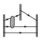
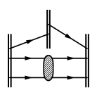
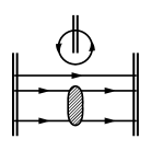
(A)                                          (B)                                          (C)

Figure 1: Graphical representation of the typical contributions to the W2W nucleon electro-magnetic three point function. The double lined “walls” correspond to the spatial Fourier integration. The dashed ellipse denotes the four quark (zero-mode) instanton interaction. The nucleon is excited at the left, struck by the virtual photon in the middle and absorbed at the right. Two contributions to the connected three-point function are shown. Diagram (A) probes the diquark content of the nucleon, whereas in diagram (B), the photon interacts with the remaining quark. Diagram (C) is disconnected, where the photon probes the sea quark content of the nucleon.

III Single-Instanton contributions

In this section, we use the SIA to evaluate the single-instanton contribution to the correlators (4), (5) and (12). The SIA is an effective theory of the instanton vacuum, in which the degrees of freedom of the closest pseudo-particle are kept explicitly into account, while the contribution from all other pseudo-particles in the vacuum is included into one effective parameter, $m^{*}\simeq$ 85 MeV. Such a parameter, which was rigorously defined and calculated in sia for different ensembles, depends only on the two phenomenological parameters of the ILM, i.e. the instanton size $\bar{\rho}$ and density $\bar{n}$.

The main advantage of the SIA is that quark propagator in the single-instanton back-ground has a simple analytical form brown78 . It consists of a zero-mode part and a non-zero mode part, $S^{I}(x,y)=S^{I}_{zm}(x,y)+S^{I}_{nzm}(x,y)$. The accuracy of the SIA was analyzed in detail in sia ; 3ptILM . It was shown that the approach is reliable only if the relevant Green functions receive maximal contribution from the zero-mode part of the propagator. In fact, the additional $\gamma_{4}$ matrix in (4), (5) and (12) has been inserted in order to meet such a requirement.

In this work, we choose to further simplify the calculation by adopting the so-called ”zero-mode approximation”, in which the non-zero mode part of the propagator is replaced by the free one, $S^{I}(x,y)\simeq S^{I}_{zm}(x,y)+S_{0}(x,y)$. Such an approximation corresponds to accounting for the ’t Hooft interaction, and neglecting other residual instanton-induced interactions, which are generally sub-leading. Indeed, in  3ptILM it was shown that the zero-mode approximation is very accurate in the case of the nucleon three- and two-point functions which we are considering.

Finally, it is convenient to use the regular gauge and work directly in a time-momentum representation of the Green functions. To this end, one expresses Eqs. (14) and (15) in terms of “wall-to-wall” (W2W) propagators, defined as the spatial Fourier transforms of the point-to-point (P2P) quark propagators:

$$S(t^{\prime},{\bf p^{\prime}};t,{\bf p})\equiv\int d^{3}{\bf x}\,d^{3}{\bf y}\,e^{i\,{\bf p^{\prime}}\cdot{\bf y}-i\,{\bf p}\cdot{\bf x}}\,S(y,x).$$ (16)

This is achieved by insertions of appropriate delta-functions at each vertex. The convenience of the time-momentum representation resides in the fact that the W2W quark propagators in the single-instanton back-ground have been calculated analytically pionFF and are smooth, non-oscillatory exponential or Bessel functions. The massless free W2W quark propagator is given by

$$S_{0}(t^{\prime},{\bf p^{\prime}};t,{\bf p})=(2\pi)^{3}\,\delta^{(3)}({\bf p^{\prime}}-{\bf p})\,\frac{e^{-|{\bf p}|\,|t^{\prime}-t|}}{2}\,u_{\mu}\gamma_{\mu},\quad$$ (17)

where $u_{4}=-1$ and $u_{l}=-i\,p_{l}/|{\bf p}|$, for $l=1,2,3$. The zero-mode W2W quark propagator in the regular gauge is given by:

$$S^{I(A)}_{zm}(t^{\prime},{\bf p^{\prime}};t,{\bf p}) = \frac{2\rho^{2}}{m^{\star}}\,f(t^{\prime},{\bf p^{\prime}};t,{\bf p})\,{\bf W}^{I(A)},$$ (18)

$$f(t^{\prime},{\bf p^{\prime}};t,{\bf p}) \equiv e^{i\,({\bf p^{\prime}}-{\bf p})\cdot{\bf z}}\,K_{0}\bigl{(}|{\bf p^{\prime}}|\,\sqrt{(t^{\prime}-z_{4})^{2}+\rho^{2}}\bigr{)}\,K_{0}\bigl{(}|{\bf p}|\,\sqrt{(t-z_{4})^{2}+\rho^{2}}\bigr{)},$$ (19)

$${\bf W}^{I(A)} \equiv \gamma_{\mu}\,\gamma_{\nu}\,\frac{1\pm\gamma_{5}}{2}\,\tau_{\mu}^{\mp}\,\tau_{\nu}^{\pm},$$ (20)

where $z_{\mu}=({\bf z},z_{4})$ denotes the instanton position, $m^{\star}$ is the effective parameter discussed above, and $\tau_{\mu}^{\pm}=({\bf\tau},\mp i)$ are color matrices.

The calculation of the correlation functions (4), (5) and (12) is performed by substituting (17) and (18) in the traces arising from Wick contractions. The quantum average is carried-out by integrating over the instanton color orientation, position, and size. The integral over the color orientation is trivial, while that over instanton position generates a delta-function which accounts for total momentum conservation. As expected, the introduction of an instanton-induced interaction generates an extra loop-integral, over the momentum exchanged through the field of the instanton. Despite the presence of loops, all diagrams are finite, as the instanton finite size provides a natural ultra-violet cut-off. The integral over the instanton size is weighted by a distribution function. In this work we assume a simple delta-function distribution $d(\rho)=\bar{n}\,\delta(\rho-\bar{\rho})$. Alternatively, one could use a fit of the instanton size distributions obtained from lattice simulations (for a compilation of results see Negele ). In a previous work we have verified that these two choices essentially give the same result pionFF .

The SIA is reliable only if the correlation functions are dominated by the contribution of the closest instanton. This condition is clearly not satisfied when the distance covered by the quarks becomes much larger than the typical distance between two neighbor instantons. Previous studies sia ; 3ptILM have shown that P2P Green functions obtained analytically in the SIA quantitatively agree with those obtained numerically in the full instanton back-ground, if the distance between the quark source and the quark sink is smaller than $\sim~{}1$ fm for two-point functions and than $\sim~{}1.8$ fm, for three-point functions.

On the other hand, we do not expect the SIA calculation of the W2W correlators to be reliable for all values of the momentum $\bf{p}$, even for small Euclidean times $t$. In fact, if the momentum is small the spatial Fourier transform (16) receives non-negligible contributions from P2P propagators connecting very distant points on the walls. However, for $|\bf{p}|$ larger than a GeV or so, only points at the distance smaller than roughly one inverse GeV from the time axis will contribute to the Fourier transform, and the SIA is applicable.

The physical reason why at large $Q^{2}$ single-instanton effects dominate over many-instanton contributions is the following. In Minkowsky space, instantons correspond to quantum fluctuations related to tunneling between degenerate classical vacua of QCD. At large momentum transfer, one can imagine computing the the form factor in an infinite-momentum frame, where the nucleon approaches the speed of light. Following the same argument of Feynmann’s parton model, one concludes that in this frame the dynamics of the nucleon is frozen. As a result of such a time dilation, during the scattering process quarks experience the consequences of - at most - a single tunneling event, i.e. of a single instanton.

In summary, the feasibility of SIA calculations relies on the existence of a range of time and momentum, where the closest instanton contribution is dominant and the ground-state is isolated. Previous studies sia ; 3ptILM ; mymasses have shown that, for the electro-magnetic three-point functions (4) and (5), this is achieved if one chooses $t$ to be $0.8~{}\textrm{fm}\lesssim t\lesssim~{}1~{}\textrm{fm}$ and restricts to the kinematic regime $|\bf{p}|\gtrsim~{}1-2~{}\textrm{GeV}$.

In order to compare SIA predictions against experiment we shall first compute the nucleon coupling constant and mass from the two-point function. Then, we shall use these values to extract the form factors from the three-point functions. All analytic results are collected in the appendix.

III.1 Nucleon mass and coupling constant in the SIA

In order to extract the nucleon mass and coupling constant in the SIA, we have evaluated the two-point function (12) for $t=0.9~{}\textrm{fm}$ and $|{\bf p}|\gtrsim 1~{}\textrm{GeV}$.

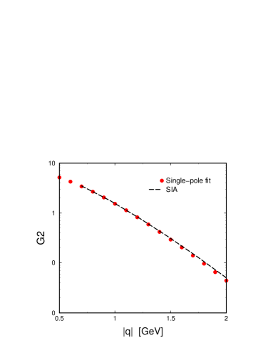
Figure 2: (Color online) The nucleon two-point function, with $t$=0.9 fm (in units of $10^{6}~{}GeV^{9}$). The dashed line denotes the SIA prediction, the points represent the single-pole fit (13), with $\Lambda_{\textrm{sc}}=0.030~{}\textrm{GeV}^{3}$ and $M=1.10$ GeV

In Fig. 2 we show the SIA prediction for ${\bf G2}(t,{\bf q})$, and compare it with the single-pole fit from Eq. (13), with $M=1.10$ GeV and $\Lambda_{\textrm{sc}}=0.030~{}\textrm{GeV}^{3}$. The agreement between SIA and the single-pole fit is very good, indicating that, for these values of time and momenta, the nucleon state has been isolated.

III.2 Proton form factors in the SIA

After having extracted the nucleon mass and coupling, we are now in condition to discuss the single-instanton contribution to the proton form factors, which are obtained from the correlation functions (7),(9), (10) and (11), at $t=0.9~{}\textrm{fm}$. These theoretical predictions are affected by the errors generated by the numerical multi-dimentional loop integration and by the uncertainty on the best-fit values for $M$ and $\Lambda_{\textrm{sc}}$. The overall error is estimated to be smaller than $5\%$.

The SIA results for the Sachs form factors of the proton are presented in Fig. 3A and compared to experimental data JLAB1 ; JLAB2 ; PGEGMexp . At relatively large momenta ( $Q^{2}\gtrsim~{}3~{}\textrm{GeV}^{2}$ ), where the approach is supposed to work, we observe a good agreement between SIA theoretical calculations and experiment.

In Fig. 3B we show the single-instanton contribution to the the ratio of magnetic and electric form factors. Also in this case, we observe that theoretical calculations converge toward the experimental data, in the large-momentum transfer regime. However, we observe that at low-momentum transfer not only is the SIA curve very far from experiment, but also its trend is opposite.

These results have several implications. On the one hand, we find that single-instanton effects provide the right amount of non-perturbative short-distance dynamics needed to explain the observed Sachs form factors at large momentum transfer. On the other hand, we see that the behavior of both the electric and the magnetic form factors at low- and intermediate-momentum transfer cannot be understood in terms of the interaction of the partons with a single instanton. In such a kinematic regime, form factors are expected to be very sensitive to many-instanton effects and possibly to other non-perturbative interactions.

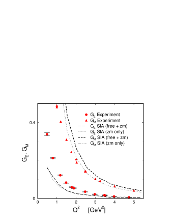
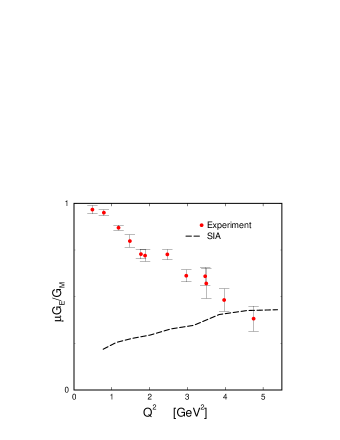
(A)                                                      (B)

Figure 3: (Color online)
(A) SIA predictions for the proton Sachs form factors compared to experimental data JLAB1 ; JLAB2 ; PGEGMexp . The experimental points for electric form factor above $Q^{2}=0.5~{}\textrm{GeV}^{2}$ are obtained from the JLAB data for $\mu~{}G_{E}(Q^{2})/G_{M}(Q^{2})$, using a dipole fit for the magnetic form factor.
(B) SIA prediction for the electric over magnetic form factors, compared to recent JLAB data obtained by recoil polarization method JLAB1 ; JLAB2 .

Let us now discuss the SIA results for the Dirac and Pauli form factors, which are reported in Fig.s (4) and (5) and compared with the fit of the experimental results. We observe that single-instanton effects are sufficient to explain with impressive accuracy the Dirac form factor, from low- to high- $Q^{2}$. Notice that, at the largest momentum available $Q^{2}\simeq~{}5.6~{}\textrm{GeV}^{2}$, the slope of the function $Q^{4}~{}F_{1}(Q^{2})$ is still larger than zero. On the other hand, we recall that in pQCD this combination should be a constant, modulo logarithmic corrections. Hence, we conclude that single-instanton effects provide the right amount of dynamics required to explain the deviation from the perturbative behavior of the Dirac form factor.

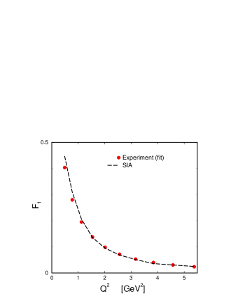
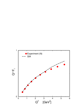
(A)                                                      (B)

Figure 4: (Color online)
(A) Dirac form factor of the proton evaluated in the SIA and compared to a phenomenological fit of the experimental data obtained as follows. In (2) the magnetic form factor is fitted with the traditional dipole formula $\mu^{-1}~{}G_{M}^{fit}=G_{dip}(Q^{2})=1/(1+Q^{2}/0.71)^{2}$. The electric form factor is obtained from $G_{E}^{fit}(Q^{2})=G_{dip}(Q^{2})\times(1.-0.13\,(Q^{2}-0.04))$, where the second factor parametrizes the JLAB data for $\mu\,G_{M}/G_{E}$.
(B) $Q^{4}$ times the Dirac form factor in the SIA and compared to a phenomenological fit of the experimental data. Perturbative QCD counting rules predict $Q^{4}\,F_{1}(Q^{2})\sim$ const.

The SIA prediction for the proton Pauli form factor is reported in Fig. 5 and compared to a fit of the experimental data. In this case, the performance of the SIA at low-momentum transfer is worse than in the case of the Dirac form factor.

It is natural to ask why the same approach performs differently in the two cases. We recall that the SIA is an effective theory of the ILM which can be used to account for instanton effects only in the limit of large momentum transfer. Therefore, the fact that the SIA prediction deviates from the data at small momentum tranfer does not necessarily imply that the instanton model is in disagreement with experiment. In order to check the ILM against low-energy experimental data one necessarily needs to perform a many-instanton calculation.

With this in mind, let us compare the definitions of the Dirac and Pauli form factors, in terms of three-point correlation functions, Eq.s (10) and (11). We observe that the $F_{2}(Q^{2})$ is obtained from a difference of correlation functions of comparable magnitude (recall that ${\bf G3}^{p(n)}_{F_{2}}$ is negative definite), while $F_{1}(Q^{2})$ is related to the sum of the same quantities. Notice also that in the combination leading to $F_{2}(Q^{2})$ the contribution of the magnetic correlator is weighted by the inverse of $Q^{2}$, (through the factor $1/\tau$) which enhances the low-momentum modes, for which the SIA becomes inaccurate. From this observations it follows that the systematic error caused by the use of the SIA in the intermediate- and low- momentum regime is larger in the case of the Pauli form factor than in the case of the Dirac form factor.

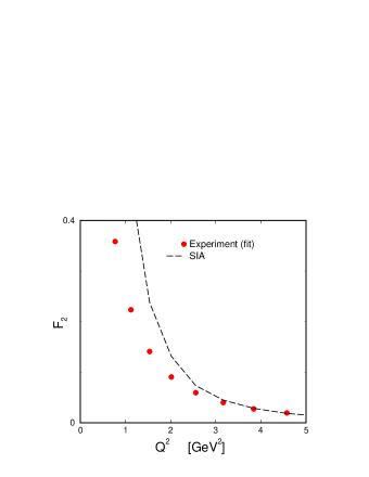
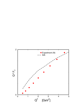
(A)                                                      (B)

Figure 5: (Color online)
(A) Pauli form factor of the proton evaluated in the SIA and compared to a phenomenological fit of the experimental data obtained as follows. In (2) the magnetic form factor is fitted with the traditional dipole formula $\mu^{-1}\,G_{M}^{fit}=G_{dip}(Q^{2})=1/(1+Q^{2}/0.71)^{2}$. The electric form factor is obtained from $G_{E}^{fit}(Q^{2})=G_{dip}(Q^{2})\times(1.-0.13\,(Q^{2}-0.04))$, where the second factor parametrizes the JLAB data for $\mu\,G_{M}/G_{E}$.
(B) $Q^{6}$ times the Pauli form factor of the proton in the SIA and compared to a phenomenological fit of the experimental data. Perturbative QCD at lowest-twist predicts $Q^{6}\,F_{2}(Q^{2})\sim$ const, modulo logarithmic corrections.

In the present calculations, all perturbative fluctuations have been neglected. It is therefore important to have at least an estimate of the magnitude of these contributions. To this end, in Fig. 3A we compare the complete SIA results with the predictions obtained by retaining only the zero-mode part of the propagator. The difference between these two curves comes from free diagrams. By definition of perturbation theory, the contribution from free diagrams has to be larger than the perturbative corrections to them. So by comparing free versus zero-mode contributions, we can estimate the importance of perturbative fluctuations, relative to the non-perturbative effects we have accounted for. In all cases considered, we found that the instanton-induced contributions represent the dominant dynamical effect.

In summary, we have observed that SIA is able to reproduce the Sachs form factor in the regime where it is applicable, i.e. at large momentum transfer. On the other hand, the approach misses important dynamics in the low- and intermediate-momentum transfer, where many-instanton effects have to be included. Interestingly, we have observed that such many-body contributions are not important in the Dirac form factor, which is extremely well reproduced in the SIA, from rather small to large $Q^{2}$.

III.3 Neutron Form Factors in the SIA

The result of the SIA calculations of the neutron electro-magnetic form factors are presented in Fig. 6 and compared with the experimental data.

As in the case of the proton, we observe that single-instanton effects can explain the data on magnetic form factor in the large momentum transfer regime. On the other hand, the electric form factor is known only at small momentum transfer, where the SIA is not reliable. In this case, the SIA undershoots the experimental data by a factor two or so. Clearly, in order to test the validity of the ILM with such a form factor, we need to include many-instanton effects.

The SIA predictions for the neutron Pauli and Dirac form factors, which are also known only at small momentum transfer, are presented for completeness in Fig. 7 and compared against experimental data. In these cases, we observe that the agreement between SIA and these low-energy data is indeed quite poor.

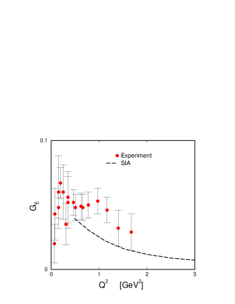
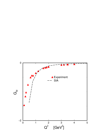
(A)                                                      (B)

Figure 6: (Color online)
(A) Electric form factor of the neutron evaluated in the SIA and compared to experimental data NGEexp .
(B) Magnetic form factor of the neutron evaluated in the SIA and compared to experimental data NGEexp .

In general, we have found that single-instanton effects alone are not sufficient to explain the available low-energy information on the form factors of the neutron.

IV Many-Instanton Contributions

In the previous section we have analyzed the single-instanton contribution to the form factors of the nucleon. In general, we observed a good agreement with experimental data, in the large momentum transfer regime. On the other hand, we have verified that at low-momentum transfer the single-instanton effects are sub-leading, as expected. Thus, in order to address the question whether also the low-energy data can be explained by the ’t Hooft interaction, we need to account for many-instanton degrees of freedom explicitly. To do so, we face the problem of computing the relevant correlation functions in the full instanton liquid vacuum, i.e. to all orders in the ’t Hooft interaction.

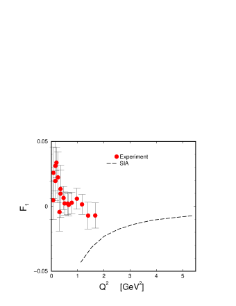
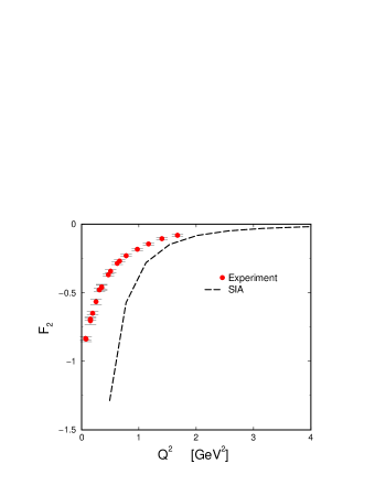
(A)                                                      (B)

Figure 7: (Color online)
(A) Dirac form factor of the neutron evaluated in the SIA and compared to experimental data. The experimental curve has been obtained by assuming that the magnetic form factors follows a dipole formula and taking the electric form factor form experiment
(B) Pauli form factor of the neutron evaluated in the SIA and compared to experimental data. The experimental curve has been obtained by assuming that the magnetic form factors follows a dipole formula and taking the electric form factor form experiment.

Such ILM calculations can be performed by exploiting the analogy between the Euclidean generating functional and the partition function of a statistical ensemble shuryakrev , in close analogy with what is usually done in lattice simulations. After the integral over the fermionic degrees of freedom is carried out explicitly, one computes expectation values of the resulting Wick contractions (14) by performing a Montecarlo average over the configurations of an ensemble of instantons and anti-instantons. In the Random Instanton Liquid (RILM), the density and size of the pseudo-particles is kept fixed, while their position in a periodic box and their color orientation is generated according to a random distribution.

In this framework, P2P correlators can be evaluated accurately in a few hours on a regular work-station. Unfortunately, the W2W correlators which are needed in order to extract the form factors are much harder to compute numerically. Indeed, many simplifications which make the SIA approach particularly convenient do not occur in a multi-instanton back-ground. For example, since at the one-instanton level the W2W quark propagator in the instanton back-ground is known in a closed form, one can carry out calculations analytically, working directly in a time-momentum representation. On the other hand, in a multi-instanton back-ground the quark propagator is obtained by inverting numerically the Dirac operator, and this operation is done in coordinate representation. Hence, one is left to computing numerically the six-dimensional integration in Eq.s (4) and (5). Furthermore, such an integration is complicated by the nasty oscillatory behavior of the integrand, introduced by the phases of the Fourier transform.

As a result of these facts, while P2P correlators can be evaluated on an ordinary single-processor computer, W2W correlators typically call for a multi-processor computation. But even on a very powerful parallel machine, an accurate evaluation of the form factors at large momentum transfer is still very hard to achieve, because in such a kinematic regime the integrand is oscillating very fast. In this section, we propose a strategy to overcome these problems.

We begin by analyzing the many-instanton contribution to the electric form factors, for which an important simplification occurs, as we shall see below. As a first step, we rewrite (4) as:

$${\bf G3}^{p(n)}_{E}(t,{\bf q},{\bf P})=\int d^{3}{\bf x}\,d^{3}{\bf y}\,e^{-i\,{\bf q}\cdot{\bf y}+i\,{\bf P}\cdot{\bf x}}\,\langle 0|\,\text{Tr}\,[\,\eta_{\text{sc}}^{p(n)}(2\,t,{\bf 0})\,J_{4}^{em}(t,{\bf y})\,\bar{\eta}_{\text{sc}}^{p(n)}(0,{\bf x})\,\gamma_{4}\,]|0\rangle.$$

(21)

Note that charge conservation implies the identity:

$${\bf G3}^{p(n)}_{E}(t,{\bf 0},{\bf P})={\bf G2}(2t,{\bf P})$$ (22)

which can be useful to test the accuracy of the numerical integration. We can now eliminate one of the complex phases by setting ${\bf P}=0$, which corresponds to going to the nucleon’s rest frame. At large Euclidean times, the resulting Green’s function has the following spectral representation:

$${\bf G3}^{p(n)}_{E}(t,{\bf q};{\bf 0}) \rightarrow \Lambda^{2}_{\text{sc}}\,\frac{\omega_{\bf{q}}+M}{\omega_{{\bf q}}}\,e^{-\,\omega_{{\bf q}}\,t}\,e^{-M\,t}G^{p(n)}_{\text{E}}(Q^{2}).$$ (23)

Now we observe that two of the three integrals in $d^{3}{\bf y}$ can be performed analytically, exploiting the fact that the above Green’s function is invariant under spatial rotations. We obtain:

$${\bf G3}^{p(n)}_{E}(t,{\bf q},{\bf 0})=\frac{4\,\pi}{|{\bf q}|}\,\int\,d|{\bf y}|\,|{\bf y}|\sin(|{\bf q}|\,|{\bf y}|)\,{\bf\Gamma 3}_{E}^{p(n)}(t,|{\bf y}|,{\bf 0}),$$ (24)

where we have introduced the “charge distribution Green’s function”:

$${\bf\Gamma 3}_{E}^{p(n)}(t,{\bf y},{\bf P})=\int\frac{d^{3}{\bf k}}{(2\,\pi)^{3}}\,{\bf G3}_{E}^{p(n)}(t,{\bf k},{\bf P})\,e^{i\,{\bf k}\cdot{\bf y}}.$$ (25)

${\bf\Gamma 3}^{p(n)}(t,{\bf y},{\bf 0})$ represents the probability amplitude for one of the three quarks which were created at an initial time in a state with with quantum numbers of the proton (neutron) and vanishing total momentum, to absorb a photon at a distance ${\bf y}$ from the origin of the center of mass frame, at a later time $t$. When the Euclidean time becomes large such a Green function encodes the information about the charge distribution of the nucleon.

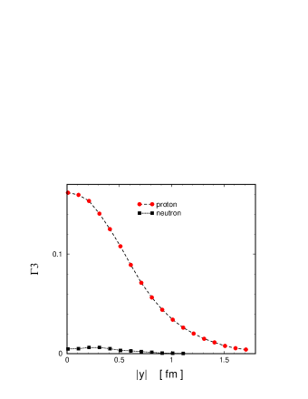
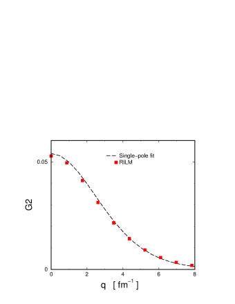
(A)                                                      (B)

Figure 8: (Color online)
(A): The charge distribution Green’s function ${\bf\Gamma 3}(t,|{\bf y}|,{\bf 0})$ for proton (circles) and nucleon (squares), evaluated in the RILM for $t=0.9~{}\textrm{fm}$.
(B): Two-point function of the nucleon in the RILM (points), compared to a single-pole fit (dashed line), ${\bf G2}_{fit}(t,|{\bf q}|)=2\,\Lambda^{2}\,e^{-t\,\sqrt{{\bf q}^{2}+M^{2}}}$ with $t=0.9~{}\textrm{fm}$.

Calculating numerically ${\bf\Gamma 3}^{p(n)}(t,|{\bf y}|,{\bf 0})$ for several values of $|{\bf y}|$ is not computationally very challenging, because it requires only a three-dimensional integration over the spatial position of the source and involves no oscillating phase. This problem can be handled with traditional adaptive Montecarlo methods, and takes a few days of computation on a regular single-processor machine. Then, for the final integration in $d\,|{\bf y}|$, we can make use of the one-dimensional integration routines which are optimized for fast-oscillating functions.

We have evaluated the function ${\bf\Gamma 3}(t,{\bf y},{\bf 0})$ in the RILM by averaging over configurations of 252 pseudo-particles of size $\rho=0.33~{}\textrm{fm}$, in a periodic box of volume $(3.6^{3}\times 5.4)~{}\textrm{fm}^{4}$. Like in lattice simulations, we have used a rather large current quark mass (70 MeV), in order to avoid finite-volume artifacts. The results for ${\bf\Gamma 3}(t,|{\bf y}|,{\bf 0})$ for different values of $|{\bf y}|$ are plotted in Fig (8) A. The final one-dimensional integration in (24) has be handled with a Gauss quadrature routine, combined with a polynomial interpolation of the integrand.

In order to extract the form factor, we have adopted the ratio of three- and two-point functions similar to the one suggested in draper :

$$G_{E}(Q^{2})\lim_{t\to\infty}\frac{2~{}\omega_{q}}{M+\omega_{q}}\frac{{\bf G3}_{E}(t,{\bf q},{\bf 0})}{{\bf G2}(2t,{\bf q})}\,\frac{{\bf G2}(t,{\bf q})}{{\bf G2}(t,{\bf 0})}.$$ (26)

IV.1 Nucleon Mass in the ILM

As in the previous SIA calculation, before extracting the form factor we need to verify that, at the Euclidean time we work at ( $t=0.9~{}\textrm{fm}$ ), the contribution of the nucleon pole to the two-point function has been isolated. To this end, in Fig. 8 B we compare our numerical results in the RILM with a single-particle fit from (13). The mass extracted from the fit is $M=1.15~{}\textrm{GeV}$, in good agreement with previous estimates in the RILM corrbaryons ; mymasses .

IV.2 Proton Form Factors in the ILM

The result of our calculation of the proton electric form factor in the RILM is presented in Fig. 9, where it is compared with experimental data and with the SIA curve. We observe a very good agreement between theory and experiment. In particular, the inclusion of many-instanton effects allows to explain the experimental data in the low-momentum regime, while at large momentum transfer the RILM gives results completely consistent with the simple single-instanton calculation. Quite remarkably, we find that the RILM prediction follows a dipole-fit at low-momenta, but falls-off faster at large momentum transfer, in agreement with what is observed in the recoil polarization measurements. Notice that this property of the form factor could not be understood at the level of the interaction of partons with a single-instanton (Fig. 3 B).

From the low-momentum points we can extract the proton charge radius, which falls slightly short of the experimental value: $\langle~{}R_{E\,(RILM)}^{2}\rangle=(0.76~{}\textrm{fm})^{2}$ (to be compared with $\langle R_{E\,(\exp.)}^{2}\rangle=(0.81~{}\textrm{fm})^{2}~{}$).

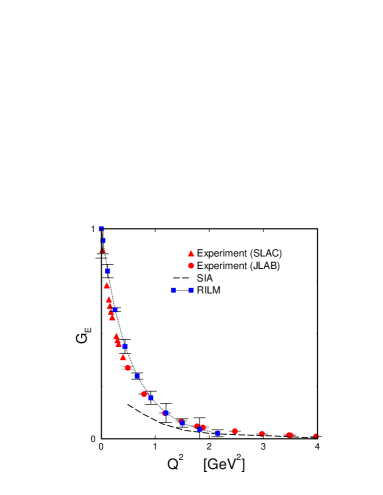
Figure 9: (Color online)
(A): Electric form factor of the proton in the ILM and from experiment. Triangles are low-energy SLAC data, which follow a dipole fit. Circles are experimental data obtained from the recent JLAB result for $G_{E}/G_{M}$, assuming a dipole fit for the magnetic form factor. Squares are result of many-instanton simulations in the RILM, and the dashed line is the SIA curve.

The fact that we obtain a slightly small charge radius is not surprising. Indeed, on the one hand we recall that in the present calculation we have used quarks of mass of about 70 MeV, corresponding to a rather heavy nucleon ($M=1.15~{}\textrm{GeV}$). On the other hand, we have neglected fermionically disconnected graphs, which encode some of the sea contribution (notice however that some “pion cloud” contribution is present through the Z-graphs).

In the previous section, we have shown that the proton Dirac form factor is completely saturated by the one-instanton contribution, already at relatively low momenta ($Q\gtrsim 0.5~{}\textrm{GeV}^{2}$). We can use this result, to combine the RILM result for $G_{E}(Q^{2})$ and the SIA result for $F_{1}(Q^{2})$ and obtain the Magnetic and the Pauli form factor of the proton in the ILM, for $Q\gtrsim 0.5~{}\textrm{GeV}^{2}$. The results for such form factors are reported in Fig. 10. Also in these two cases we see that the inclusion of many-instanton effects is sufficient to explain the low-energy data.

IV.3 Electric Form Factor of the Neutron in the ILM

The results from the electric form factor of the neutron are shown in Fig. 11. In this case, the agreement with experiment is somewhat worse than the corresponding results for the proton electric form factor. Our theoretical prediction undershoots experimental data by a factor 2 or so. We believe that this discrepancy is mainly due to the absence of disconnected graphs. Clearly, the relative contribution of such SU(3) breaking effects are much more important in the case of the neutron, which has a very small electric form factor compared to the proton. This hypothesis is supported by the fact that in Lattice1 , the disconnected diagrams were calculated in lattice QCD and found to give a contribution of the order of $50\%$ to the form factor. A systematic study of the sea contribution coming from disconnected graphs to several low-energy observables is currently in progress PJD .

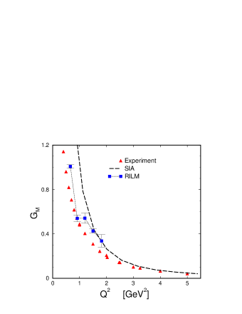
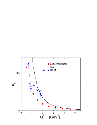
(A)                                                      (B)

Figure 10: (Color online)
(A): Magnetic form factor of the proton in the ILM (squares) and from experiment (triangles). The ILM curve has been obtained by combining the analytical SIA prediction for the Dirac form factor $F_{1}$ with the numerical RILM results for $G_{E}$.
(B): Pauli Form Factor of the proton in the ILM. The circles are obtained from a fit of the experimental data. Squares is the ILM prediction, obtained by combining RILM results for $G_{E}$ with the SIA results for $F_{1}$.

V Conclusions

The present study was motivated by the observation that recent JLAB data show that electro-magnetic form factors are very sensitive to some short-distance non-perturbative dynamics. Instantons are known to play the leading role in the spontaneous breaking of chiral symmetry and in the saturation of the chiral anomaly, i.e. in two very important non-perturbative phenomena which occur at the GeV scale. In a previous analysis we had showed that instantons saturate the the pion charged form factor and, at the same time, explain why the perturbative regime is reached much earlier in the $\gamma\,\gamma^{*}\to~{}\pi_{0}$ transition from factor. In this work, we have asked whether they can also explain some existing puzzles concerning the nucleon form factors.

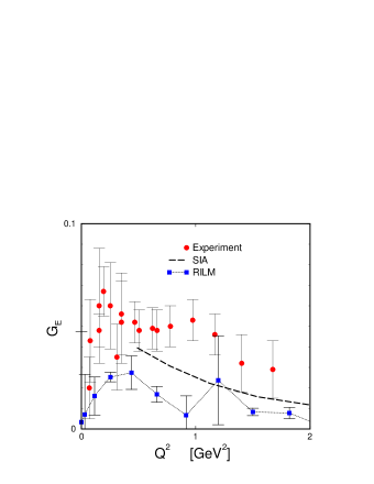
Figure 11: (Color online)
Electric form factor of the neutron in the RILM and from experiment NGEexp . Circles are experimental data, squares are RILM point, while the dashed line is the SIA curve.

We have found that large momentum transfer data of Sachs as well as Pauli and Dirac form factors can be already reproduced by accounting for the scattering of the partons on a single-instanton. These calculations have been carried-out in the SIA. On the other hand, form factors at low-momenta cannot be calculated in the SIA because, in such a kinematic regime, many-instanton effects are very important. The only exception is the proton Dirac form factor, which is saturated by one instanton, already at relatively low momentum transfer ($Q^{2}\sim 0.5~{}\textrm{GeV}^{2}$).

We have evaluated numerically the electric form factors in the full instanton vacuum, i.e. to all orders in the ’t Hooft interaction, using the RILM. In the case of the proton, we have found that RILM predictions are consistent with SIA calculations at large momentum transfer and quantitatively reproduce the available body of experimental data. In particular, we have shown that in the ILM the electric form factor follows a dipole fit at low momenta, but falls-off faster at large momenta, in quantitative agreement with the recent JLAB results. On the other hand, the electric form factor of the neutron seems to be rather sensitive to fermionically disconnected graphs and SU(3) breaking effects, which have been neglected in the present approach.

We have combined our SIA result for the proton Dirac form factor, with our numerical RILM results for the electric form factors and obtained predictions for the magnetic and Pauli form factors. As in the previous cases, we have found very good agreement with experiment for all proton form factors. In the future we are planning to use the framework developed in this work to investigate the role of the pion cloud in low-energy observables.

APPENDIX: ANALYTIC RESULTS IN THE SIA

Every where, we choose ${\bf q}$ pointing along the $\hat{1}$ direction: ${\bf q}=(q,0,0)$. Let us define the following functions:

$$\xi^{-}(t):=\sqrt{(t-z_{4})^{2}+\bar{\rho}^{2}}$$

$$\xi^{+}(t):=\sqrt{(t+z_{4})^{2}+\bar{\rho}^{2}}$$

$$\xi^{0}(t):=\sqrt{t^{2}+\bar{\rho}^{2}}$$ (27)

V.1 Two-point function

The SIA result for the two-point function defined in (12) is:

$${\bf G2}(t,{\bf q})=\frac{32\,\bar{n}\,\rho^{4}}{m^{*\,2}\,\pi^{6}}\int_{0}^{\infty}d|{\bf k}|~{}d|{\bf l}|~{}d|{\bf m}|~{}|{\bf m}|^{2}\,|{\bf k}|^{2}\,|{\bf l}|^{2}\int_{-1}^{1}dc_{k}~{}dc_{l}~{}dc_{m}\int_{-\infty}^{\infty}dz_{4}~{}\left(A+B\right),$$

where

$$A:=2\,K_{0}(|{\bf k}|\,\xi^{-}(t/2))\,K_{0}(|{\bf m}|\,\xi^{+}(t/2))\,K_{0}(\chi_{m}^{-}\,\xi^{+}(t/2))\,K_{0}(\chi_{k}^{-}\,\xi^{-}(t/2))\,e^{-t\,\chi_{q}^{+}},$$

$$B:=\,K_{0}(|{\bf k}|\,\xi^{-}(t/2))\,K_{0}(|{\bf m}|\,\xi^{+}(t/2))\,K_{0}(\chi_{m}^{+}\,\xi^{+}(t/2))\,K_{0}(\chi_{k}^{+}\,\xi^{-}(t/2))\,e^{-t\,\chi_{q}^{-}},$$

and

$$\chi_{Q}^{+}:=\sqrt{|{\bf l}|^{2}+|{\bf q}|^{2}+2\,|{\bf q}|\,|{\bf l}|\,c_{l}}$$

$$\chi_{Q}^{-}:=\sqrt{|{\bf l}|^{2}+|{\bf q}|^{2}-2\,|{\bf q}|\,|{\bf l}|\,c_{l}}$$

$$\chi_{m}^{+}:=\sqrt{|{\bf l}|^{2}+|{\bf m}^{2}+2\,|{\bf m}\,|{\bf l}|\,c_{m}}$$

$$\chi_{m}^{-}:=\sqrt{|{\bf l}|^{2}+|{\bf m}^{2}-2\,|{\bf m}\,|{\bf l}|\,c_{m}}$$

$$\chi_{k}^{+}:=\sqrt{|{\bf l}|^{2}+|{\bf k}|^{2}+2\,|{\bf k}|\,|{\bf l}|\,c_{k}}$$

$$\chi_{k}^{-}:=\sqrt{|{\bf l}|^{2}+|{\bf k}|^{2}-2\,|{\bf k}|\,|{\bf l}|\,c_{k}}.$$

V.2 Magnetic Three-point Function

The SIA result for the proton (neutron) magnetic three-point function defined in (5) is:

$${\bf G3}^{p(n)}_{M}(t,{\bf q})=\frac{\bar{n}\,\bar{\rho}^{4}}{m^{*\,2}}\,\int\frac{d^{3}{\bf k}}{(2\,\pi)^{3}}\int\frac{d^{3}{\bf l}}{(2\,\pi)^{3}}\int\frac{d^{3}{\bf m}}{(2\,\pi)^{3}}\,\left[\frac{2}{3}\,U^{M}(D)({\bf k},{\bf l},{\bf m})-\frac{1}{3}\,D^{M}(U)({\bf k},{\bf l},{\bf m})\right],$$

where

$$U^{M}({\bf k},{\bf l},{\bf m}):=U^{M}_{1}+U^{M}_{2}+U^{M}_{3}+U^{M}_{4},$$

and

$$D^{M}({\bf k},{\bf l},{\bf m}):=D^{M}_{1}+D^{M}_{2}.$$

The functions $U^{M}_{1-4}$ correspond to sets of diagrams in which the virtual photon is absorbed by a $u$-quark. They are defined as follows:

• $U^{M}_{1}:=u^{M}_{1a}+u^{M}_{1b}+u^{M}_{1c},$

  $$u^{M}_{1a}:=-256\,\frac{m_{3}^{2}+m_{1}^{2}+qm_{1}-m_{2}^{2}-|{\bf m}||{\bf m}+{\bf q}|}{|{\bf m}||{\bf m}+{\bf q}|}\,e^{-t\ (|{\bf m}+{\bf q}|+|{\bf m}|)}\,K_{0}(|{\bf k}|\,\xi^{-}(t))\,$$

  $$\times\,K_{0}(|{\bf l}|\,\xi^{+}(t))\,K_{0}(|{\bf q}/2+{\bf m}+{\bf k}|\,\xi^{-}(t))\,K_{0}(|{\bf q}/2+{\bf m}+{\bf l}|\,\xi^{+}(t)).$$

  $$u^{M}_{1b}:=+256\,\frac{l_{2}\,k_{2}}{|{\bf l}||{\bf k}+{\bf q}|}\,e^{-t(|{\bf k}+{\bf q}|+2|{\bf l}|)}\,K_{0}(|{\bf k}|\,\xi^{0}(t))\,K_{0}(|{\bf q}/2+{\bf l}+{\bf k}|\,\xi^{-}(t))$$

  $$\times\,K_{0}(|{\bf m}|\,\xi^{+}(t))\,K_{0}(|{\bf q}/2+{\bf m}+{\bf l}|\,\xi^{+}(t)).$$

  $$u^{M}_{1c}:=+256\,\frac{-m_{1}\,l_{1}+m_{2}\,l_{2}-m_{3}\,l_{3}+|{\bf m}||{\bf l}|}{|{\bf m}||{\bf l}|}\,e^{-t(|{\bf m}|+2|{\bf l}|)}\,K_{0}(|{\bf m}+{\bf q}|\,\xi^{0}(t))$$

  $$\times K_{0}(|{\bf k}|\,\xi^{-}(t))\,K_{0}(|{\bf q}/2-{\bf l}-{\bf k}|\,\xi^{-}(t))\,K_{0}(|{\bf q}/2+{\bf m}+{\bf l}|\,\xi^{+}(t))$$

• $U^{M}_{2}:=u^{M}_{2a}+u^{M}_{2b},$

  $$u^{M}_{2a}:=-1024\frac{m_{2}(l_{2}+m_{2})}{|{\bf q}/2+{\bf m}+{\bf l}||{\bf m}|}\,e^{-t(2|{\bf q}/2+{\bf m}+{\bf l}|+|{\bf m}|)}\,K_{0}(|{\bf q}-{\bf k}+{\bf l}+{\bf m}|\,\xi^{-}(t))$$

  $$\times\,K_{0}(|{\bf m+q}|\,\xi^{0}(t))\,K_{0}(|{\bf k}|\,\xi^{-}(t))\,K_{0}(|{\bf l}|\,\xi^{+}(t))$$

  $$u^{M}_{2b}:=-1024\,\frac{(l_{2}-k_{2}+m_{2})\,(m_{2}+l_{2})}{|{\bf q}/2+{\bf m}+{\bf l}||{\bf q}-{\bf k}+{\bf m}+{\bf l}|}e^{-t(2|{\bf q}/2+{\bf m}+{\bf l}|+|{\bf m}+{\bf q}-{\bf k}+{\bf l}|)}\,K_{0}(|{\bf k}|\,\xi^{-}(t))$$

  $$\times\,K_{0}(|{\bf l}+{\bf m}-{\bf k}|\,\xi^{0}(t))\,K_{0}(|{\bf l}|\,\xi^{+}(t))\,K_{0}(|{\bf m}|\,\xi^{+}(t))$$

• $U^{M}_{3}:=u^{M}_{3a}+u^{M}_{3b}+u^{M}_{3\,c}$,

  $$u^{M}_{3a}:=+\frac{128}{|{\bf m}+{\bf l}-{\bf k}+{\bf q}||{\bf m}+{\bf q}/2+{\bf l}|}(-2l_{1}k_{1}+2l_{1}^{2}+3qm_{1}-2m_{1}k_{1}+4m_{1}l_{1}+2m_{1}^{2}$$

  $$-qk_{1}+2ql_{1}+3ql_{1}-2l_{3}k_{3}+2l_{3}^{2}-2m_{3}k_{3}+4m_{3}l_{3}+q^{2}-2l_{2}^{2}-2m_{2}^{2}$$

  $$-4m_{2}l_{2}+2m_{2}k_{2}+2l_{2}k_{2}+2m_{3}^{2}+2\,|{\bf q}/2+{\bf m}+{\bf l}||{\bf q}+{\bf m}+{\bf l}-{\bf k}|)\,$$

  $$\times\,e^{-t(2|{\bf q}/2+{\bf m}+{\bf l}|+|{\bf q}-{\bf k}+{\bf l}+{\bf m}|)}K_{0}(|{\bf m}|\,\xi^{+}(t))K_{0}(|{\bf l}|\,\xi^{+}(t))\,K_{0}(|{\bf k}|\,\xi^{-}(t))\,K_{0}(|{\bf m}+{\bf l}-{\bf k}|\,\xi^{0}(t))$$

  $$u^{M}_{3b}:=-256\,\frac{(l_{2}+m_{2})\,m_{2}}{|{\bf m}||{\bf q}/2+{\bf m}+{\bf l}|}\,e^{-t\,(2|{\bf m}+{\bf l}+{\bf q}/2|+|{\bf m}|)}\,K_{0}(|{\bf k}|\,\xi^{-}(t))\,K_{0}(|{\bf l}|\,\xi^{+}(t))\,$$

  $$K_{0}(|{\bf q}+{\bf m}|\,\xi^{0}(t))K_{0}(|{\bf q}-{\bf k}+{\bf m}+{\bf l}|\,\xi^{-}(t))$$

  $$u^{M}_{3c}:=-256\,\frac{m_{1}^{2}-m_{2}^{2}+m_{3}^{2}+q\,m_{1}-|{\bf m}||{\bf m}+{\bf q}|}{|{\bf m}||{\bf m}+{\bf q}|}e^{-t(2|{\bf m}+{\bf q}|+|{\bf m}|)}K_{0}(|{\bf l}|\,\xi^{+}(t))\,$$

  $$K_{0}(|{\bf q}/2+{\bf m}+{\bf l}|\,\xi^{+}(t))\,K_{0}(|{\bf k}|\,\xi^{-}(t))\,K_{0}(|{\bf q}/2+{\bf m}+{\bf k}|\,\xi^{-}(t))$$

• $U^{M}_{4}:=u^{M}_{4a},$

  $$u^{M}_{4a}:=-1024\,\frac{(m_{1}^{2}-m_{2}^{2}+m_{3}^{2}+q\,m_{1}-|{\bf m}||{\bf m}+{\bf q}|)\,m_{2}}{|{\bf m}||{\bf q}+{\bf m}|}\,e^{-t\,(|{\bf m}+{\bf q}|+|{\bf m}|)}K_{0}(|{\bf k}|\,\xi^{-}(t))\,$$

  $$K_{0}(|{\bf q}/2+{\bf m}+{\bf k}|\,\xi^{-}(t))\,K_{0}(|{\bf q}/2+{\bf m}+{\bf l}|\,\xi^{+}(t))K_{0}(|{\bf l}|\,\xi^{+}(t))$$

The functions $D^{M}_{1-2}$ correspond to sets of diagrams in which the photon is absorbed by a $d$-quark. They are defined as follows:

• $D^{M}_{1}:=d^{M}_{1a}+d^{M}_{1b}$

  $$d^{M}_{1a}:=-1024\,\frac{m_{2}\,(m_{2}+l_{2})}{|{\bf m}||{\bf m}+{\bf q}/2+{\bf l}|}\,e^{-t(|{\bf m}|+2\,|{\bf q}/2+{\bf l}+{\bf m}|)}K_{0}(|{\bf m}+{\bf q}|\,\xi^{0}(t))$$

  $$K_{0}(|{\bf l}|\,\xi^{+}(t))\,K_{0}(|{\bf k}|\,\xi^{-}(t))\,K_{0}(|{\bf q}-{\bf k}+{\bf m}+{\bf l}|\,\xi^{-}(t))$$

  $$d^{M}_{1b}:=+1024\,\frac{(m_{2}+l_{2})\,(k_{2}-l_{2}-m_{2})}{|{\bf m}+{\bf q}/2+{\bf l}|+|{\bf q}+{\bf l}+{\bf m}-{\bf k}|}\,e^{-t(2|{\bf m}+{\bf q}/2+{\bf l}|+|{\bf q}+{\bf l}+{\bf m}-{\bf k}|)}$$

  $$K_{0}(|{\bf m}+{\bf l}-{\bf k}|\,\xi^{0}(t))\,K_{0}(|{\bf m}|\,\xi^{+}(t))\,K_{0}(|{\bf k}|\,\xi^{-}(t))\,K_{0}(|{\bf l}|,\xi^{+}(t))$$

• $D^{M}_{2}:=d^{M}_{2a}+d^{M}_{2b}+d^{M}_{2c}+d^{M}_{2d}$,

  $$d^{M}_{2a}:=+256\,\frac{{\bf m}\,{\bf l}-|{\bf l}||{\bf m}|}{|{\bf m}|\,|{\bf l}|}\,e^{-t(|{\bf m}|+2|{\bf l}|)}K_{0}(|{\bf m}+{\bf q}|\,\xi^{0}(t))\,K_{0}(|{\bf k}|\,\xi^{+}(t))\,$$

  $$K_{0}(|{\bf q}/2+{\bf m}+{\bf l}|\,\xi^{+}(t))\,K_{0}(|{\bf q}/2-{\bf k}-{\bf l}|\,\xi^{-}(t))$$

  $$d^{M}_{2b}:=-256\,\frac{m_{2}\,(m_{2}+l_{2})}{|{\bf m}+{\bf q}/2+{\bf l}||{\bf m}|}\,e^{-t(2|{\bf m}+{\bf q}/2+{\bf l}|+|{\bf m}|)}K_{0}(|{\bf m}+{\bf l}-{\bf k}+{\bf q}|\,\xi^{-}(t))$$

  $$K_{0}(|{\bf m}+{\bf q}|\,\xi^{0}(t))\,K_{0}(|{\bf k}|\,\xi^{-}(t))\,K_{0}(|{\bf l}|,\xi^{+}(t))$$

  $$d^{M}_{2c}:=+256\,\frac{l_{2}\,k_{2}}{|{\bf k}+{\bf q}||{\bf l}|}\,e^{-t(|{\bf q}+{\bf k}|+2|{\bf l}|)}K_{0}(|{\bf l}+{\bf k}+{\bf q}/2|\,\xi^{-}(t))\,K_{0}(|{\bf m}|\,\xi^{+}(t))\,$$

  $$K_{0}(|{\bf k}|\,\xi^{0}(t))\,K_{0}(|{\bf q}/2+{\bf m}+{\bf l}|,\xi^{+}(t))$$

  $$d^{M}_{2d}:=-\frac{256}{2|{\bf m}+{\bf l}-{\bf k}+{\bf q}||{\bf q}/2+m+{\bf l}|}\,e^{-t(|{\bf m}+{\bf l}-{\bf k}+{\bf q}|+2|{\bf l}+{\bf q}/2+{\bf m}|)}\,K_{0}(|{\bf l}|\,\xi^{+}(t))\,$$

  $$\times\,(2m_{1}^{2}+3m_{1}q-qk_{1}-2m_{1}k_{1}-2l_{1}k_{1}-2m_{3}k_{3}-2l_{3}k_{3}+q^{2}+$$

  $$3l_{1}q+4l_{1}m_{1}+2l_{1}^{2}+2m_{3}^{2}+4l_{3}m_{3}+2l_{3}^{2}+4l_{2}m_{2}$$

  $$-2m_{2}k_{2}-2l_{2}k_{2}+2l_{2}^{2}+2m_{2}^{2}+2|{\bf q}/2+{\bf m}+{\bf l}|\,|{\bf q}+{\bf m}+{\bf l}-{\bf k}|)$$

  $$\times\,K_{0}(|{\bf m}-{\bf k}+{\bf l}|\,\xi^{0}(t))\,K_{0}(|{\bf k}|\,\xi^{-}(t))\,K_{0}(|{\bf m}|,\xi^{+}(t))$$

V.3 Electric Three-point Function

The proton (neutron) electric three-point function reads:

$${\bf G3}^{p(n)}_{E}(t,{\bf q})=\frac{\bar{n}\,\bar{\rho}^{4}}{m^{*\,2}}\,\int\frac{d^{3}{\bf k}}{(2\,\pi)^{3}}\int\frac{d^{3}{\bf l}}{(2\,\pi)^{3}}\int\frac{d^{3}{\bf m}}{(2\,\pi)^{3}}\,\left[\frac{2}{3}\,U^{E}(D)({\bf k},{\bf l},{\bf m})-\frac{1}{3}\,D^{E}(U)({\bf k},{\bf l},{\bf m})\right]$$

where,

$$U^{E}({\bf k},{\bf l},{\bf m}):=U^{E}_{1}+U^{E}_{2}+U^{E}_{3}+U^{E}_{4},$$ (28)

and

$$D^{E}({\bf k},{\bf l},{\bf m}):=D^{E}_{1}+D^{E}_{2}.$$

As in the case of the magnetic three-point function, $U^{E}_{1-4}$ correspond to sets of diagrams in which the photon is absorbed by a $u$-quark. They are defined as follows:

• $U^{E}_{1}:=u^{E}_{1a}+u^{E}_{1b}+u^{E}_{1c},$

  $$u^{E}_{1a}:=-256\,\frac{{\bf m}^{2}+qm_{1}+|{\bf m}||{\bf m}+{\bf q}|}{|{\bf m}||{\bf m}+{\bf q}|}\,e^{-t\ (|{\bf m}+{\bf q}|+|{\bf m}|)}\,K_{0}(|{\bf k}|\,\xi^{-}(t))\,$$

  $$\times\,K_{0}(|{\bf l}|\,\xi^{+}(t))\,K_{0}(|{\bf q}/2+{\bf m}+{\bf k}|\,\xi^{-}(t))\,K_{0}(|{\bf q}/2+{\bf m}+{\bf l}|\,\xi^{+}(t))$$

  $$u^{E}_{1b}:=-256\,e^{-t(|{\bf k}+{\bf q}|+2|{\bf l}|)}\,K_{0}(|{\bf k}|\,\xi^{0}(t))\,K_{0}(|{\bf q}/2+{\bf l}+{\bf k}|\,\xi^{-}(t))$$

  $$\times\,K_{0}(|{\bf m}|\,\xi^{+}(t))\,K_{0}(|{\bf q}/2+{\bf m}+{\bf l}|\,\xi^{+}(t))$$

  $$u^{E}_{1c}:=-256\,\frac{{\bf l}{\bf m}+|{\bf m}||{\bf l}|}{|{\bf m}||{\bf l}|}\,e^{-t(|{\bf m}|+2|{\bf l}|)}\,K_{0}(|{\bf m}+{\bf q}|\,\xi^{0}(t))$$

  $$\times K_{0}(|{\bf k}|\,\xi^{-}(t))\,K_{0}(|{\bf q}/2-{\bf l}-{\bf k}|\,\xi^{-}(t))\,K_{0}(|{\bf q}/2+{\bf m}+{\bf l}|\,\xi^{+}(t))$$

• $U^{E}_{2}:=u^{E}_{2a}+u^{E}_{2b},$

  $$u^{E}_{2a}:=-1024\,e^{-t(2|{\bf q}/2+{\bf m}+{\bf l}|+|{\bf m}|)}\,K_{0}(|{\bf q}-{\bf k}+{\bf l}+{\bf m}|\,\xi^{-}(t))$$

  $$\times\,K_{0}(|{\bf m+q}|\,\xi^{0}(t))\,K_{0}(|{\bf k}|\,\xi^{-}(t))\,K_{0}(|{\bf l}|\,\xi^{+}(t))$$

  $$u^{E}_{2b}:=-1024\,e^{-t(2|{\bf q}/2+{\bf m}+{\bf l}|+|{\bf m}+{\bf q}-{\bf k}+{\bf l}|)}\,K_{0}(|{\bf k}|\,\xi^{-}(t))$$

  $$\times\,K_{0}(|{\bf l}+{\bf m}-{\bf k}|\,\xi^{0}(t))\,K_{0}(|{\bf l}|\,\xi^{+}(t))\,K_{0}(|{\bf m}|\,\xi^{+}(t))$$

• $U^{E}_{3}:=u^{E}_{3a}+u^{E}_{3b}+u^{E}_{3\,c}$,

  $$u^{E}_{3a}:=+\frac{128}{|{\bf m}+{\bf l}-{\bf k}+{\bf q}||{\bf m}+{\bf q}/2+{\bf l}|}\,e^{-t(2|{\bf q}/2+{\bf m}+{\bf l}|+|{\bf q}-{\bf k}+{\bf l}+{\bf m}|)}$$

  $$\times\,(2{\bf m}^{2}+2{\bf l}^{2}+4{\bf m}{\bf l}-2{\bf l}{\bf k}-2{\bf m}{\bf k}+3qm_{1}+3ql_{1}+q^{2}-qk_{1}$$

  $$+2\,|{\bf q}/2+{\bf m}+{\bf l}||{\bf q}+{\bf m}+{\bf l}-{\bf k}|)\,\,K_{0}(|{\bf m}|\,\xi^{+}(t))$$

  $$\times K_{0}(|{\bf l}|\,\xi^{+}(t))\,K_{0}(|{\bf k}|\,\xi^{-}(t))\,K_{0}(|{\bf m}+{\bf l}-{\bf k}|\,\xi^{0}(t))$$

  $$u^{E}_{3b}:=-256\,e^{-t\,(2|{\bf m}+{\bf l}+{\bf q}/2|+|{\bf m}|)}\,K_{0}(|{\bf k}|\,\xi^{-}(t))\,K_{0}(|{\bf l}|\,\xi^{+}(t))\,$$

  $$K_{0}(|{\bf q}+{\bf m}|\,\xi^{0}(t))K_{0}(|{\bf q}-{\bf k}+{\bf m}+{\bf l}|\,\xi^{-}(t))$$

  $$u^{E}_{3c}:=-256\,\frac{{\bf m}^{2}+q\,m_{1}+|{\bf m}||{\bf m}+{\bf q}|}{|{\bf m}||{\bf m}+{\bf q}|}e^{-t(2|{\bf m}+{\bf q}|+|{\bf m}|)}K_{0}(|{\bf l}|\,\xi^{+}(t))\,$$

  $$K_{0}(|{\bf q}/2+{\bf m}+{\bf l}|\,\xi^{+}(t))\,K_{0}(|{\bf k}|\,\xi^{-}(t))\,K_{0}(|{\bf q}/2+{\bf m}+{\bf k}|\,\xi^{-}(t))$$

• $U^{E}_{4}:=u^{E}_{4a},$

  $$u^{E}_{4a}:=-1024\,\frac{{\bf m}^{2}+q\,m_{1}+|{\bf m}||{\bf m}+{\bf q}|}{|{\bf m}||{\bf q}+{\bf m}|}\,e^{-t\,(|{\bf m}+{\bf q}|+|{\bf m}|)}K_{0}(|{\bf k}|\,\xi^{-}(t))\,$$

  $$K_{0}(|{\bf q}/2+{\bf m}+{\bf k}|\,\xi^{-}(t))\,K_{0}(|{\bf q}/2+{\bf m}+{\bf l}|\,\xi^{+}(t))K_{0}(|{\bf l}|\,\xi^{+}(t))$$

The functions $D^{E}_{1-2}$ correspond to sets of diagrams in which the photon is absorbed by a $d$-quark. They are defined as follows:

• $D^{E}_{1}:=d^{E}_{1a}+d^{E}_{1b}$

  $$d^{E}_{1a}:=-1024\,e^{-t(|{\bf m}|+2\,|{\bf q}/2+{\bf l}+{\bf m}|)}K_{0}(|{\bf m}+{\bf q}|\,\xi^{0}(t))\,K_{0}(|{\bf l}|\,\xi^{+}(t))$$

  $$K_{0}(|{\bf k}|\,\xi^{-}(t))\,K_{0}(|{\bf q}-{\bf k}+{\bf m}+{\bf l}|\,\xi^{-}(t))$$

  $$d^{E}_{1b}:=-1024\,\,e^{-t(2|{\bf m}+{\bf q}/2+{\bf l}|+|{\bf q}+{\bf l}+{\bf m}-{\bf k}|)}\,K_{0}(|{\bf m}+{\bf l}-{\bf k}|\,\xi^{0}(t))$$

  $$K_{0}(|{\bf m}|\,\xi^{+}(t))\,K_{0}(|{\bf k}|\,\xi^{-}(t))\,K_{0}(|{\bf l}|\,\xi^{+}(t))$$

• $D^{E}_{2}:=d^{E}_{2a}+d^{E}_{2b}+d^{E}_{2c}+d^{E}_{2d}$,

  $$d^{E}_{2a}:=+256\,\frac{{\bf m}\,{\bf l}-|{\bf l}||{\bf m}|}{|{\bf m}|\,|{\bf l}|}\,e^{-t(|{\bf m}|+2|{\bf l}|)}K_{0}(|{\bf m}+{\bf q}|\,\xi^{0}(t))\,K_{0}(|{\bf k}|\,\xi^{+}(t))\,$$

  $$K_{0}(|{\bf q}/2+{\bf m}+{\bf l}|\,\xi^{+}(t))\,K_{0}(|{\bf q}/2-{\bf k}-{\bf l}|\,\xi^{-}(t))$$

  $$d^{E}_{2b}:=-256\,\,e^{-t(2|{\bf m}+{\bf q}/2+{\bf l}|+|{\bf m}|)}K_{0}(|{\bf m}+{\bf l}-{\bf k}+{\bf q}|\,\xi^{-}(t))$$

  $$K_{0}(|{\bf m}+{\bf q}|\,\xi^{0}(t))\,K_{0}(|{\bf k}|\,\xi^{-}(t))\,K_{0}(|{\bf l}|\,\xi^{+}(t))$$

  $$d^{E}_{2c}:=-256\,e^{-t(|{\bf q}+{\bf k}|+2|{\bf l}|)}K_{0}(|{\bf l}+{\bf k}+{\bf q}/2|\,\xi^{-}(t))\,K_{0}(|{\bf m}|\,\xi^{+}(t))\,$$

  $$K_{0}(|{\bf k}|\,\xi^{0}(t))\,K_{0}(|{\bf q}/2+{\bf m}+{\bf l}|\,\xi^{+}(t))$$

  $$d^{E}_{2d}:=\frac{-256}{2|{\bf m}+{\bf l}-{\bf k}+{\bf q}||{\bf q}/2+m+{\bf l}|}\,e^{-t(|{\bf m}+{\bf l}-{\bf k}+{\bf q}|+2|{\bf l}+{\bf q}/2+{\bf m}|)}\,K_{0}(|{\bf l}|\,\xi^{+}(t))\,$$

  $$\times\,(2m_{1}^{2}+3m_{1}q-qk_{1}-2m_{1}k_{1}-2l_{1}k_{1}-2m_{3}k_{3}-2l_{3}k_{3}+q^{2}+$$

  $$3l_{1}q+4l_{1}m_{1}+2l_{1}^{2}+2m_{3}^{2}+4l_{3}m_{3}+2l_{3}^{2}+4l_{2}m_{2}$$

  $$-2m_{2}k_{2}-2l_{2}k_{2}+2l_{2}^{2}+2m_{2}^{2}+2|{\bf q}/2+{\bf m}+{\bf l}|\,|{\bf q}+{\bf m}+{\bf l}-{\bf k}|)$$

  $$\times\,K_{0}(|{\bf m}-{\bf k}+{\bf l}|\,\xi^{0}(t))\,K_{0}(|{\bf k}|\,\xi^{-}(t))\,K_{0}(|{\bf m}|\,\xi^{+}(t))$$

References

• (1) J. Volmer et al. [The Jefferson Laboratory $F_{\pi}$ Collaboration], Phys. Rev. Lett. 86 (2001) 1713.
• (2) M.K. Jones, et al., Phys. Rev. Lett. 84 (2000) 1398.
• (3) O. Gayou, et al., Phys. Rev. Lett. 88 (2002) 092301.
• (4) S.J. Brodsky and G.R. Farrar, Phys. Rev. Lett. 31 (1973) 1153.
• (5) A. Belitsky, X. Ji and F. Yuan, Phys. Rev. Lett. 91 (2003) 092003.
• (6) M.C. Chu, J.M. Grandy, S. Huang, and J.W. Negele, Phys. Rev. D49 (1994) 6039.
• (7) G. ’t Hooft, Phys. Rev. Lett. 37 (1976) 8.
G. ’t Hooft, Phys. Rev. D14 (1976) 3432.
• (8) D. Diakonov, Chiral symmetry breaking by instantons, Lectures given at the ”Enrico Fermi” school in Physics, Varenna, June 25-27 1995, hep-ph/9602375.
• (9) T. Schäfer and E.V. Shuryak, Rev. Mod. Phys. 70 (1998) 323.
• (10) T.A. DeGrand and A. Hasenfratz, Phys. Rev. D64 (2001) 034512.
• (11) P. Faccioli and T.A. DeGrand, Phys. Rev. Lett. 91 (2003) 182001.
• (12) E.V. Shuryak, Nucl. Phys. B214 (1982) 237.
• (13) F. Iachello, A.D. Jackson and A. Lande, Phys. Lett. B43 (1973) 191.
B.Q. Ma, D. Qing and I. Smidt, Phys. Rev. C65 (2002) 035205.
G.A. Miller, Phys. Rev. C66 (2002) 032201.
C.V. Christov, A.Z. Gorzki, K. Goeke and P.V. Pobilitza, Nucl. Phys. A592 (1995) 513.
• (14) H. Forkel and M. Nielsen, Phys. Lett. B345 (1995) 55.
• (15) V.V. Braguta and A.I. Onishchenko, hep-ph/0311146.
• (16) A. Blotz and E.V. Shuryak, Phys. Rev. D55 (1997) 4055.
• (17) P. Faccioli and E.V. Shuryak, Phys. Rev. D65 (2002) 076002.
• (18) P. Faccioli and E.V. Shuryak, Phys. Rev. D64 (2001) 114020.
• (19) P. Faccioli, Phys. Rev. D65 (2002) 094014.
• (20) P. Faccioli, A. Schwenk and E.V. Shuryak, Phys. Rev. D67 (2003) 113009.
• (21) A. E. Dorokhov, JETP Lett.  77, 63 (2003) [Pisma Zh. Eksp. Teor. Fiz.  77, 68 (2003)]
• (22) P. Faccioli, A. Schwenk and E.V. Shuryak, Phys. Lett. B549 (2002) 93.
• (23) L.S. Brown, R.D. Carlitz, D.B. Craemer and C. Lee, Phys. Rev. D17 (1978) 1583.
• (24) L.E. Price, et al. Phys. Rev. D4 (1971) 45.
P. Bosted et al., Phys. Rev. Lett 68 (1992) 3841.
R.C. Walker et al., Phys. Rev. D49 (1994), 5671.
• (25) M. Meyerhoff et al., Phys. Lett. B327 (1994) 201.
J. Becker et al., Eur. Phys. J. A6 (1999) 329.
C. Herberg et al., Eur. Phys. J. A5 (1999) 131.
M. Orstick et al., Phys. Rev. Lett. 83 (1999) 276.
I. Passchier et al., Phys. Rev. Lett. 82 (1999) 4988.
D. Rohe et al., Phys. Rev. Lett. 83 (1999) 4257.
H. Zhu et al., Phys. Rev. Lett. 87 (2001) 081801.
• (26) J.W. Negele, Nucl. Phys. Proc. Suppl. 73 (1999) 92.
• (27) P. Faccioli, J. Negele and D. Renner, in preparation.
• (28) G. Martinelli and C.T. Sachrajda, Nucl. Phys. B316 (1989) 355.
• (29) W. Wilcox, T. Draper and K.F. Liu, Phys. Rev. D46 (1992) 1109.
• (30) T. Schäfer, E.V. Shuryak and J.J.M. Verbaarschot, Nucl. Phys. B412 (1994) 143.
• (31) S.J. Dong, K.F. Liu and A.G. Williams, Phys. Rev. D58 (1998) 074504.