The $\tt BABAYAGA$ event generator

Abstract

The program $\tt BABAYAGA$ is an event generator for QED processes at flavour factories, mainly intended for luminosity measurement of $e^{+}e^{-}$ colliders in the center of mass range 1-10 GeV. Recently, the $\pi^{+}\pi^{-}$ channel has been added as well. The relevant (photonic) radiative corrections are simulated by means of a Parton Shower in QED. The theoretical precision of the approach is estimated and some phenomenological results are discussed.

1 Introduction

The precise determination of the machine luminosity is an important ingredient for the successful achievement of the physics programme at the $e^{+}e^{-}$ colliders running with center of mass energy in the range of the low lying hadronic resonances (1 - 10 GeV).

One of the most important challenges is the precise measure of the $R$ ratio, by means of the energy scan or the radiative return method. The aim is to reduce the theoretical error on the hadronic contribution to the vacuum polarization, which will reflect on the error of the anomalous magnetic moment of the muon $a_{\mu}$ and the QED coupling constant at the $Z$ peak $\alpha_{QED}(M_{Z}^{2})$ [1]. Actually, the $R$ measurement is going to become a precision measurement [2, 3] and it will give a stringent test of the Standard Model predictions.

In this perspective, a precise knowledge of the cross section for QED processes for luminometry, expecially for Bhabha scattering, and their Monte Carlo (MC) simulation are crucial. The theoretical accuracy should be better than $0.5\%$.

2 The theoretical approach in $\tt BABAYAGA$

$\tt BABAYAGA$ [4, 5] is a Monte Carlo event generator for the simulation of QED and $\pi^{+}\pi^{-}$ processes at flavour factories.

In order to achieve an accurate prediction of the cross sections of the QED processes, the relevant radiative correction (RC) have to be accounted for, and, in particular, photon radiation effects must be included in the calculation.

2.1 The QED Structure Functions

The corrected cross section and the event generation can be obtained according to the following master formula (see [4] and references therein):

$$\sigma(s)=\int dx_{1}dx_{2}dy_{1}dy_{2}\int d\Omega\times$$

$$D(x_{1},Q^{2})D(x_{2},Q^{2})D(y_{1},Q^{2})D(y_{2},Q^{2})\times$$

$$\frac{d\sigma_{0}(x_{1}x_{2}s)}{d\Omega}\Theta(cuts)$$ (1)

The previous equation is used in $\tt BABAYAGA$ for the generation of the processes $e^{+}e^{-}\to e^{+}e^{-}(n\gamma)$, $\to\mu^{+}\mu^{-}(n\gamma)$, $\to\gamma\gamma(n\gamma)$ and $\to\pi^{+}\pi^{-}(n\gamma)$. The last channel has been recently implemented and, in this case, only photons coming from initial state are accounted for.

In eq. 1, the Born-like cross section for the process $d\sigma_{0}/d\Omega$ is convoluted with the QED non-singlet Structure Functions (SF’s) $D(x,Q^{2})$, which are the solution of the Dokshitzer-Gribov-Lipatov-Altarelli-Parisi (DGLAP) [6] equation in QED

$$Q^{2}\frac{\partial}{\partial Q^{2}}D(x,Q^{2})=\frac{\alpha}{2\pi}\int_{x}^{1}\frac{dy}{y}P_{+}(y)D(\frac{x}{y},Q^{2})$$

$$P_{+}(x)=\frac{1+x^{2}}{1-x}-\delta(1-x)\int_{0}^{1}dtP(t)$$ (2)

where $P_{+}(x)$ is the regularized Altarelli-Parisi vertex. The SF’s in eq. 1 account for photon radiation emitted by both initial-state (ISR) and final-state (FSR) fermions. The SF’s allow to include the universal virtual and real photonic corrections, up to all orders of perturbation theory. Strictly speaking, radiation in eq. 1 is collinear to the emitting fermions.

It is possible to go beyond the collinear approximation by solving the DGLAP equation by means of a MC algorithm, the so-called Parton Shower algorithm (PS), which is discussed in the next section.

2.2 The Parton Shower algorithm

The Parton Shower is a MC algorithm which solves exactly the DGLAP equation (see references in [4]) and it originates from an iterative solution of eq. 2

$$D(x,Q^{2})=\Pi(Q^{2},m^{2})\delta(1-x)$$

$$+\frac{\alpha}{2\pi}\int_{m^{2}}^{s}\Pi(Q^{2},s^{\prime})\frac{ds^{\prime}}{s^{\prime}}\Pi(s^{\prime},m^{2})\times$$

$$\times\int_{0}^{x_{+}}dyP(y)\delta(x-y)+$$

$$+\ 2\ photons+\cdots$$ (3)

In eq. 3, $\Pi(Q^{2},m^{2})=e^{-\frac{\alpha}{2\pi}\log(\frac{Q^{2}}{m^{2}})\int_{\epsilon}^{1}P(x)}$ is the Sudakov Form Factor, where the soft and virtual RC are exponentiated. The $Q^{2}$ scale is not a priori fixed, but it has to be chosen in order to reproduce as close as possible the leading RC contributions coming from the exact order $\alpha$ calculation. For example, for the Bhabha scattering, a reasonable choice is $Q^{2}=st/ue$, where $s$,$t$ and $u$ are the usual Mandelstam variables and $e$ is the Euler’s number.

The main advantage of this solution is that it keeps track of the number of the emitted photons and that their kinematics can be approximately recovered. Therefore, the whole branching event can be generated and the multi-photon emission can be exclusively simulated.

The generation of the photon’s momenta has to be carefully considered. As suggested by eq. 3, when the PS generates photons, their energy is extracted from the Altarelli-Parisi vertex $P(x)$, where $x$ is the energy fraction remaining to the fermion after the photon emission.

In order to generate also the angular variables, different solutions can be exploited [5], being those degrees of freedom integrated out in eqs. 2 and 3. The first possible choice is to weight the photon angles according to the leading poles which are present in the radiation matrix element. Namely, the photons’ angles can be distributed according to the following formula

$$\cos\vartheta_{\gamma}\propto\sum_{i=1,4}\frac{1}{p_{i}\cdot k}$$ (4)

where $p_{i}$ are the momenta of the charged particles and $k$ is the momentum of the generic photon. If eq. 4 can be a first approximation, it is not so accurate when photonic variables are looked at closer. In order to improve the exclusive photon generation, we can observe that in eq. 4 the interference effects between ISR and FSR are completely neglected, thus the fermions radiate independently.

The radiation coherence effects can be included if we consider the cross section for the production of $n$ photons from a generic process involving fermions as external particles. Taking the soft limit and keeping all the interference terms, the resulting formula is

$$d\sigma_{n}\approx d\sigma_{0}\frac{1}{n!}\prod_{l=1}^{n}\frac{e^{2}d^{\it 3}\mathbf{k}_{l}}{(2\pi)^{3}2k^{0}_{l}}\sum_{i,j}\frac{\eta_{i}\eta_{j}p_{i}\cdot p_{j}}{(p_{i}\cdot k_{l})(p_{j}\cdot k_{l})}$$ (5)

where $k_{l}$ and $p_{j}$ are photons and fermions momenta and $\eta_{i}=\pm 1$ is a charge factor. The angular spectrum of the photons can be directly extracted from the eq. 5. This highly enhances the reliability of the PS also in the simulation of radiative events, as will be shown in section 4.

An important point is the estimate of the physical precision of the PS approach. In order to give a consistent estimate, an $\cal{O}(\alpha)$ PS has been developed as well, which calculates the corrected cross section of eq. 1 at first order in $\alpha$ in the PS approximation. By a systematic comparison of the the $\cal{O}(\alpha)$ PS results to the exact $\cal{O}(\alpha)$ matrix element ones, the PS precision can be estimated and, in particular, the size of the $\cal{O}(\alpha)$ non-leading-log contributions missing in a pure PS approach can be quantified.

2.3 The hard scattering cross sections

The other ingredient entering eq. 1 is the “kernel” cross section, which is the Born-like cross section for the process evaluated at the reduced center of mass energy $x_{1}x_{2}s$. In $\tt BABAYAGA$, the standard formulae for Bhabha, $\gamma\gamma$ and $\mu^{+}\mu^{-}$ processes are implemented. For the $\pi^{+}\pi^{-}$ channel, the pion Form Factor as parameterized in [7] is present. The hard scattering cross section includes also vacumm polarization contributions. It is worth discussing in some details how they are treated in the last official release of $\tt BABAYAGA$ ($\tt 3.5$).

The running of $\alpha(q^{2})$ is given by

$$\alpha(q^{2})=\frac{\alpha(0)}{1-\Delta\alpha(q^{2})}$$

$$\Delta\alpha(q^{2})=\Delta\alpha_{had}^{(5)}(q^{2})+\Delta\alpha_{t}(q^{2})+$$

$$+\sum_{l}\Delta\alpha_{l}(q^{2})$$ (6)

The lepton and top quark contributions ($\Delta\alpha_{l}(q^{2})$ and $\Delta\alpha_{t}(q^{2})$) do not show any problem, being analytically calculable for any $q^{2}$ value.

The hadronic contribution $\Delta\alpha_{had}^{(5)}(q^{2})$ is calculated by means of the subroutine $\tt HADR5$ [8] (which is now superseded by a new version). This subroutine is not suited to work in the $q^{2}$ time-like region below ($40$ GeV)². As suggested by one of the authors [9], the following solution was therefore adopted: in this $q^{2}$ region, the $q^{2}$ is flipped to $-q^{2}$, in order to include at least the leading terms of the hadronic contribution to $\Delta\alpha(q^{2})$.

Recently, a new version of the routine has been written [10] with an improved treatment of the resonances region (including new experimental data) and which is suited for any $q^{2}$ value. It has been preliminarly included in the program, showing a difference on the integrated Bhabha cross section at DA$\Phi$NE energies at a few per mille level. However, a deeper look is needed and will be carried out in the next future.

3 The benchmark calculation $\tt LABSPV$

One of the crucial points to be considered is the estimate of the theoretical accuracy of the PS approach. In order to quantify the theoretical error, the independent program $\tt LABSPV$ has been derived from the code $\tt SABSPV$ [11], which was extensively used for LEP luminometry. It is not a true event generator, but it is a cross section integrator.

In $\tt LABSPV$, the exact order $\alpha$ matrix element is used, and the $\cal{O}(\alpha)$-corrected cross section is calculated according to the standard formula

$$\sigma_{exact}^{\alpha}=\sigma_{S+V}^{\alpha}(E_{\gamma}<k_{0})+\sigma_{H}^{\alpha}(E_{\gamma}>k_{0})$$ (7)

where $\sigma^{\alpha}_{S+V}$ is the soft-photon plus virtual cross section, $\sigma^{\alpha}_{H}$ is the hard-photon emission cross section and $k_{0}$ is a soft-hard radiation separator, which the total cross section does not depend on. The code $\tt LABSPV$ calculates the cross sections for the Bhabha, $\gamma\gamma$ and $\mu^{+}\mu^{-}$ (only for high energies, $E_{c.m.}\gg m_{\mu}$) processes, using matrix elements and formulae which can be found in [12, 13, 14]. In the Bhabha and $\mu^{+}\mu^{-}$ case, vacuum polarization is treated as done in $\tt BABAYAGA$.

On top of the exact $\cal{O}(\alpha)$ cross section of eq. 7, in $\tt LABSPV$, higher order leading-log QED corrections in a SF approach can be also included, according to the relation

$$\sigma^{h.o.}=\sigma_{exact}^{\alpha}-\sigma_{SF}^{\alpha}+\sigma_{SF}^{\infty}$$ (8)

where $\sigma_{SF}^{\alpha}$ is the order $\alpha$ expansion of eq. 1 and $\sigma_{SF}^{\infty}$ is eq. 1. In $\tt LABSPV$, the SF’s are an analytical solution of the QED DGLAP equation [15] and are strictly collinear. Equation 8 can be further improved if cast in the factorized form

$$\sigma^{h.o.}=\sigma_{SF}^{\infty}(1+\frac{\sigma_{exact}^{\alpha}-\sigma_{SF}^{\alpha}}{\sigma_{0}})$$ (9)

It can be shown [16] that in expression 9 the bulk of the $\alpha^{2}L$ corrections ($L$ is the collinear logarithm) are also taken into account, in addition to the exact order $\alpha$ and leading-log higher order contributions. As a consequence, the expected theoretical accuracy of this approach for cross section calculation can be estimated at the level of 0.1%.

Table 1: Comparison at different center of mass energies of the total $\gamma\gamma$ cross section between $\tt LABSPV$ and the results of ref. [13] (B. & K.)

$$\begin{array}[]{l|l|l}\hline\cr\lx@intercol\hfil\mbox{$e^{+}e^{-}\to\gamma\gamma(\gamma)$ total cross sections}\hfil\lx@intercol\\ \hline\cr\mbox{energy (GeV)}&\mbox{B. \& K.}&\mbox{{$\tt LABSPV$}}\\[2.84526pt] \hline\cr 1&2013.7&2013.6(3)\\ 3&264.90&264.92(5)\\ 5&102.58&102.59(2)\\ 7&54.82&54.82(1)\\ 10&28.184&28.182(6)\\ \hline\cr\end{array}$$

Being used as a “benchmark”, $\tt LABSPV$ has been compared to different independent calculations finding very good agreement. For example, in table 1, the total cross section for $\gamma\gamma$ is compared to the analytical results of [13].

4 Phenomenological results

4.1 Coherent Parton Shower

As discussed in paragraph 2.2, the photon angular generation can be performed in order to simulate also the ISR-FSR interference, which is neglected in a pure “leading-pole” generation. The coherence effect can be important when exclusive photon distributions are considered.

Figure 1: The photon angular distribution as obtained by the leading-pole $\cal{O}(\alpha)$ PS (red dots), the coherent $\cal{O}(\alpha)$ PS (blue dots) and the exact $\cal{O}(\alpha)$ matrix element (histogram). Cuts are given in the text.

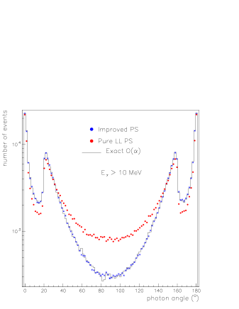
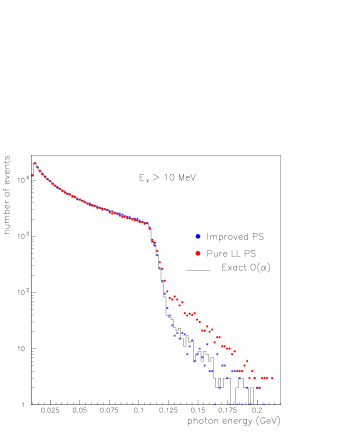
In fig. 1, the photon angular distribution is shown for $e^{+}e^{-}\to e^{+}e^{-}\gamma$ events at $\sqrt{s}=1.02$ GeV, with $20^{\circ}<\vartheta_{\pm}<160^{\circ}$, $E_{\pm}>0.4$ GeV and $E_{\gamma}>10$ MeV. The leading-pole and coherent $\cal{O}(\alpha)$ PS results obtained with $\tt BABAYAGA$ are compared to the exact $\cal{O}(\alpha)$ distribution of $\tt LABSPV$. The improvement of the coherence PS is evident. In fig. 2, the distribution of the photon energy is plotted for the same sample of events. Even if the leading-pole PS already produces a good distribution, being the photon energy driven by the Altarelli-Parisi vertex, the coherent PS is better also in the tail of the energy spectrum.

Figure 2: The photon energy distribution as obtained by the leading-pole $\cal{O}(\alpha)$ PS (red dots), the coherent $\cal{O}(\alpha)$ PS (blue dots) and the exact $\cal{O}(\alpha)$ matrix element (histogram). Cuts are given in the text.

A similar behaviour is found for the PS at all orders: in fig. 3, the angular distribution of the most energetic photon as obtained by the coherent and the leading-pole PS at all orders are compared to the exact $\cal{O}(\alpha)$ distribution (even if this is not fully consistent).

Figure 3: The most energetic photon distribution as obtained by the leading-pole PS (open circles) and the coherent PS at all orders (stars) compared exact to the $\cal{O}(\alpha)$ matrix element photon distribution (histogram).

4.2 Theoretical error

The theoretical error of $\tt BABAYAGA$ for cross section calculation can be evaluated by comparing the $\cal{O}(\alpha)$ PS to the exact matrix element of eq. 7. Actually, the main contribution to the error comes from the non-leading-log $\cal{O}(\alpha)$ terms, missing in the PS approach.

In fig. 4, the relative deviation between the inclusive Bhabha cross section obtained with $\tt BABAYAGA$ at $\cal{O}(\alpha)$ and the exact matrix element is plotted as a function of the acollinearity cut, both for the leading-pole PS and the coherent PS. The imposed experimental cuts are $\sqrt{s}=1.019$ GeV, $20^{\circ}<\vartheta_{\pm}<160^{\circ}$ (top in the figure) or $50^{\circ}<\vartheta_{\pm}<130^{\circ}$ (bottom in the figure), $E^{min}_{\pm}=0.4$ GeV.

Figure 4: Relative effects of missing $\cal{O}(\alpha)$ contributions in $\tt BABAYAGA$. Blue triangles represent the coherent PS and the red ones the leading-pole PS. See text for details.

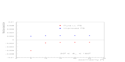
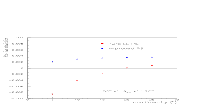
From fig. 4, it emerges that the error in $\tt BABAYAGA$ is at level of $0.5\%$ or lower. It is worth noticing that for the coherent PS the size of the missing $\cal{O}(\alpha)$ is almost constant as the cuts vary, while for the leading-pole PS it is not constant and it can become larger than $0.5\%$.

For the Bhabha case, we can fix the theoretical error of $\tt BABAYAGA$ in the calculation of the QED corrected cross section at the level of $0.5\%$.

4.3 Higher order corrections

Aiming at a high precision calculation of the QED processes cross section, higher order contributions can not be neglected, expecially if a “bare” event selection criterium is adopted and almost-elastic events are selected.

The PS allows to include higher-order corrections in a natural way. In fig. 5, the relative difference between the cross sections obtained with $\tt BABAYAGA$ at $\cal{O}(\alpha)$ and at all orders is shown. The simulation has been performed applying the same cuts as in fig. 4. As it can be seen, the higher-order contributions are quite large: they can change the cross section for an amount of $1-2\%$, depending on the cuts, and are therefore important to achieve the desired theoretical accuracy. The higher-order impact can be also estimated with $\tt LABSPV$, finding a good agreement. In the plots of figure 5, the effect of the $\alpha^{2}L$ contributions is also shown, estimated with $\tt LABSPV$. They are negligible, being below the $5\cdot 10^{-4}$.

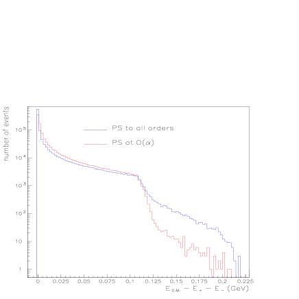
It interesting to notice that multi-photon emission has a sizeable effect also on distributions. For example, in figure 6 the distribution of radiation energy, defined as $E_{c.m.}-E_{+}-E_{-}$, is plotted and the $\cal{O}(\alpha)$ PS is compared to the all order PS.

Figure 5: Relative effects of higher-order contributions obtained with $\tt BABAYAGA$ and $\alpha^{2}L$ contribution obtained with $\tt LABSPV$. See text for details.

Figure 6: Effect of multi-photon emission on the radiation energy distribution

5 Other channels

$\tt BABAYAGA$ can generate also $\mu^{+}\mu^{-}(n\gamma)$, $\gamma\gamma(n\gamma)$ and $\pi^{+}\pi^{-}(n\gamma)$ final states, generating events according to eq. 1 and the PS algorithm.

For $\mu^{+}\mu^{-}$ and $\gamma\gamma$ processes, a study as detailed as for Bhabha process to establish the theoretical accuracy has not been performed yet, but it is planned.

As a general consideration, it should be noticed that in the benchmark program $\tt LABSPV$ the fully massive $\mu^{+}\mu^{-}(\gamma)$ exact $\cal{O}(\alpha)$ matrix element is not present and therefore it is not reliable at low energies, where the muon mass effects become important.

Concerning the $\gamma\gamma$ final state, it has to be pointed out that the PS approach suffers for double counting. In fact, the photons generated by the PS are independent from the photons of the hard scattering process: if the PS photons are allowed to go inside the phase space region of the hard scattering ones, this leads to a double counting error. However, the error can be kept small if large angle photons are selected, because PS emits photons preferably collinear to initial-state $e^{+}$ and $e^{-}$.

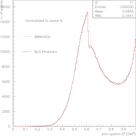
In the version $\tt 3.5$ of the program, also the $\pi^{+}\pi^{-}(n\gamma)$ channel has been added. In this case, only ISR is simulated with the PS. With the PS approach, also the radiative $\pi^{+}\pi^{-}\gamma$ event can be studied, which is extremely important for the $R$ measurement via the radiative return method. The process was added only for cross-checking purposes, being the $\tt PHOKHARA$ MC event generator [17] much more accurate for $\pi^{+}\pi^{-}\gamma$.

Nevertheless, the results of $\tt BABAYAGA$ are quite good. In figure 7, the $\pi^{+}\pi^{-}$ invariant mass distribution obtained by $\tt BABAYAGA$ is compared to the $\tt PHOKARA\ 1.0$ distribution. The imposed cuts are $\sqrt{s}=1.02$ GeV, $55^{\circ}<\vartheta_{\pm}<125^{\circ}$, $5^{\circ}<\vartheta_{\gamma}<21^{\circ}$ and $E_{\gamma}>10$ MeV.

Figure 7: $\pi^{+}\pi^{-}$ invariant mass distribution by $\tt BABAYAGA$ and $\tt PHOKHARA\ 1.0$. Cuts are given in the text.

6 Towards a new release of $\tt BABAYAGA$

Table 2: Preliminary comparisons for Bhabha cross sections (in $nb$) obtained with $\tt LABSPV$, $\tt BABAYAGA\ 3.5$ and an improved version of $\tt BABAYAGA$. Cuts are given in the text.

$$\begin{array}[]{l|l|c|c|c|c}\mbox{acceptance}&\mbox{RC}&\mbox{$\tt LABSPV$ (eq. \ref{sigmaadd})}&\mbox{$\tt LABSPV$ (eq. \ref{sigmafact})}&\mbox{{$\tt BABAYAGA\ 3.5$}}&\mbox{improved $\tt BABAYAGA$}\\ \hline\cr 55^{\circ}-125^{\circ}&\mbox{$\cal{O}(\alpha)$}&451.70(1)&&454.76(1)&451.75(1)\\ &\mbox{$\cal{O}(\alpha)$+h.o.}&456.20(2)&456.36(4)&458.86(1)&455.96(2)\\ \hline\cr 20^{\circ}-160^{\circ}&\mbox{$\cal{O}(\alpha)$}&6061.9(2)&&6088.8(1)&6062.5(2)\\ &\mbox{$\cal{O}(\alpha)$+h.o.}&6087.1(3)&6090.0(7)&6114.4(1)&6088.2(3)\\ \hline\cr\end{array}$$

As discussed in the section 4, the main source of error in a PS approach comes from the missing $\cal{O}(\alpha)$ non-log terms. It would be extremely useful to include them in the generator, in order to further reduce its theoretical error. In the measurements of the KLOE collaboration for the $R$ ratio, the theoretical error in the luminosity is going to be the dominant one [3].

When trying to include the exact $\cal{O}(\alpha)$ matrix element in the PS for exclusive event generation , different merely technical problems arise (negative weigths, higher-order not well under control, etc.). Work in this direction is in progress.

Here, we would like to show some preliminary results obtained with a new version of $\tt BABAYAGA$, where part of the exact $\cal{O}(\alpha)$ matrix element for Bhabha scattering is used.

Roughly, the idea is the following: the events are reweigthed for a (infrared-independent) factor which accounts for the difference between the exact and the PS soft-plus-virtual cross section. Radiative events should then be reweigthed with the exact $\cal{O}(\alpha)$ radiative matrix element. At present, we did not succeed to perform exactly the latter step. Nevertheless, it is possible to find out from eq. 5 a weight factor which is much closer to the exact matrix element than what is implemented in $\tt BABAYAGA\ 3.5$. The technical details will be discussed elsewhere.

It is worth stressing that this procedure is done at differential level and the order $\alpha$ expansion of the resulting cross section reproduces exactly the soft-plus-virtual cross section ($\sigma^{\alpha}_{S+V}$) of eq. 7 and “almost” exactly the hard photon term ($\sigma^{\alpha}_{H}$) of eq. 7.

In table 2, the cross section of $\tt LABSPV$, $\tt BABAYAGA\ 3.5$ and new version are compared. The applied cuts for the cross sections shown in the table are $\sqrt{s}=1.02$ GeV, $20^{\circ}<\vartheta_{\pm}<160^{\circ}$ or $55^{\circ}<\vartheta_{\pm}<125^{\circ}$, $E_{\pm}^{min}>0.408$ GeV, maximum acollinearity $\zeta_{max}=10^{\circ}$. In table 2, the vacuum polarization contributions have been switched off. The differences between the improved version of $\tt BABAYAGA$ and $\tt LABSPV$ are below the 0.1%.

7 Conclusions

The program $\tt BABAYAGA$ is a MC event generator for QED processes and $\pi^{+}\pi^{-}$ final state at flavour factories. The QED radiative corrections are included by means of a Parton Shower. The theoretical accuracy of the approach is estimated to be at $0.5\%$ for cross section calculation.

Some preliminary results have been presented of a new version of the generator, which is under development. In the next future, it will include also the exact $\cal{O}(\alpha)$ matrix element and will improve the theoretical accuracy of the approach.

8 Acknowledgments

The authors would like to thank the organizers of the SIGHAD03 Workshop for the pleasant athmosphere and the useful discussions during the workshop.

References

- [1] F. Jegerlehener, hep-ph/0310234; F. Jegerlehner, J. Phys.G 29,101 (2003).
- [2] R.R. Akhmetshin et al. [the CMD-2 collaboration], hep-ex/0308008.
- [3] A. Aloisio et al. [the KLOE collaboration], hep-ex/0307051.
- [4] C.M. Carloni Calame et al., Nucl. Phys. B 584 (2000) 459.
- [5] C.M. Carloni Calame, Phys. Lett. B 520 (2001) 16.
- [6] V.N. Gribov and L.N. Lipatov, Sov. J. Nucl. Phys. 15 (1972) 298; G. Altarelli and G. Parisi, Nucl. Phys. B 126 (1977) 298; Y.L. Dokshitzer, Sov. Phys. JETP 46 (1977) 641.
- [7] J.H. Kühn and A. Santamaria Z. Physik C 48 (445) 1990.
- [8] S. Eidelman and F. Jegerlehner Z. Physik C 67 (585) 1995.
- [9] F. Jegerlehner, private communication.
- [10] The new version is available at the web site http://www-zeuthen.desy.de/fjeger/.
- [11] M. Cacciari et al., in Report of the Working Group on Precision Calculations for the Resonance, D. Bardin, W. Hollik, G. Passarino eds., CERN Report 95-03, 389; Comput. Phys. Commun. 90 (1995) 301.
- [12] M. Caffo et al., in Physics at LEP1, G. Altarelli, R. Kleiss and C. Verzegnassi eds., CERN Report 89-08, Vol. 1, 171; M. Greco, Riv. Nuovo Cim., Vol. 11 (1988) 1.
- [13] F.A. Berends and R. Kleiss, Nucl. Phys. B 186 (1981) 22.
- [14] F.A. Berends et al., Nucl. Phys. B 202 (1981) 63.
- [15] O. Nicrosini and L. Trentadue, Phys. Lett. B 196 (1987) 551; M. Cacciari et al., Europhys. Lett.17 (1992) 123.
- [16] G. Montagna et al., Phys. Lett. B 385 (1996) 348.
- [17] G. Rodrigo et al., Eur. Phys. J.C 22, 81 (2001); G. Rodrigo et al., Eur. Phys. J. C 24 (2002) 71; H. Czyz et al., Eur. Phys. J. C 27, 563 (2003).
- [18] S. Frixione and B.R. Webber, JHEP 0206 (2002) 029.