Anomalous Flavor $\boldsymbol{U\!(1)_{\!X}}$ for Everything

Abstract

We present an ambitious model of flavor, based on an anomalous $U(1)_{X}$ gauge symmetry with one flavon, only two right-handed neutrinos and only two mass scales: $M_{grav}$ and $m_{3/2}$. In particular, there are no new scales introduced for right-handed neutrino masses. The $X$-charges of the matter fields are such that $R$-parity is conserved exactly, higher-dimensional operators are sufficiently suppressed to guarantee a proton lifetime in agreement with experiment, and the phenomenology is viable for quarks, charged leptons, as well as neutrinos. In our model one of the three light neutrinos automatically is massless. The price we have to pay for this very successful model are highly fractional $X$-charges which can likely be improved with less restrictive phenomenological ansätze for mass matrices.

1 Introduction

The fermionic mass spectrum of the standard model ($S\!M$) suggests that the entries of the quark and charged lepton Yukawa matrices exhibit hierarchical patterns. Froggatt and Nielsen (FN) in Ref. [1] presented an idea to explain these texture structures, tracing them back to a flavor $U(1)_{X}$ symmetry beyond the $S\!M$, which is broken by an $S\!M$-singlet, called the flavon. For early models see e.g. Refs. [2, 3]. Then string theory gave a theoretical motivation for the existence and the breaking scale of the $U(1)_{X}$ (in particular, it turned out that the anomalousness of the $U(1)_{X}$ is a blessing), so the FN scenario was easily embedded, see e.g. Ref. [4].

One may naturally assume that the origin of the aforementioned hierarchy also leaves its fingerprints on the other (Yukawa) coupling constants, which opens up many more applications of the FN scenario:  1.) It is tempting to use the idea of FN for investigating why $R$-parity violating Yukawa coupling constants have not led yet to the observation of exotic processes, see e.g. Refs. [6, 7]; in these models $R$-parity violating coupling constants are mostly suppressed down to phenomenologically acceptable levels (rather than them being forbidden exactly), however this will render the Lightest Supersymmetric Particle not an attractive candidate for Cold Dark Matter.  2.) Or to provide an explanation (see e.g. Ref. [8]) why (with or without grand unification) higher-dimensional genuinely supersymmetric operators like $QQQL$ do not cause a short-lived proton; after all, these operators are suppressed by just a single power of the reduced Planck scale, so the dimensionless coefficient must be adequately tiny.  3.) Furthermore, the idea of FN can easily be combined (see Ref. [9]) with the Giudice-Masiero (GM) mechanism (see Refs. [10, 11]) to naturally explain the $\mu$-term of the minimal supersymmetric extension of the $S\!M$ ($M\!S\!S\!M$).  4.) Last, but not least, neutrino data can also be interpreted in the light of the FN idea, see e.g. Ref. [12]. However, when dealing with right-handed neutrinos, the obvious question is: What distinguishes the neutrino superfield from the flavon superfield?

The aim of this note is to dovetail all of these different aspects of the FN scenario and at the same time be curmudgeonly about letting string theory introduce other beyond-$M\!S\!S\!M$ symmetries and/or particles. So our intention is to construct a minimalistic supersymmetric FN model with the following features:

• There is only one additional symmetry group beyond $SU(3)_{C}\times SU(2)_{W}\times U(1)_{Y}$ in the visible sector, namely a generation-dependent local $U(1)_{X}$. For the cancellation of $U(1)_{X}$ gauge anomalies we invoke the Green-Schwarz mechanism, see Ref. [13]. We employ the notation that a left-chiral superfield $\Phi$ carries the $U(1)_{X}$ charge $X_{\Phi}$.

• There is only one (left-chiral) flavon superfield $A$, which acquires a vacuum expectation value (VEV) $\langle A\rangle$ via the Dine-Seiberg-Wen-Witten mechanism, see Refs. [14, 15, 16, 17], thus breaking $U(1)_{X}$.

• In analogy to the three species (i.e. generations) of $X$- and $S\!M$-charged matter superfields $\{Q^{i},L^{i},\overline{U^{i}},\overline{D^{i}},\overline{E^{i}}\}$ ($i=1,2,3$), there are three species of superfields whose only gauge group is $U(1)_{X}$: the flavon superfield and two right-handed neutrino superfields $\overline{N^{I}}$ ($I=1,2$). Thus the flavon superfield is so to speak a right-handed neutrino superfield without lepton number.

• The model produces a viable phenomenology: Quark masses and mixings and charged lepton masses agree with the data, see Refs. [18, 9]; the neutrino masses and mixings are in accord with the recent measurements, see Ref. [19] and references therein; the lower bounds on proton longevity, see e.g. Ref. [20, 21], and other rare processes are satisfied; broken $R$-parity (for a review see e.g. Ref. [22]) is forbidden by virtue of the $X$-charges.

• There are only two mass scales: the mass of the gravitino $m_{3/2}\sim 1~{}$TeV (we assume gravity mediation of supersymmetry breaking, see Refs. [27, 28, 29, 30]) and the reduced Planck scale $M_{grav}\sim 2.4\times 10^{18}~{}$GeV where gravity becomes strong.^,

• $\{Q^{i},L^{i},\overline{U^{i}},\overline{D^{i}},\overline{E^{i}},H^{\mathcal{D}},H^{\mathcal{U}}\}$ are the only $S\!M$-charged superfields, and we made the (unsuccessful, due to the gravitational anomaly) attempt here that those fields together with $\{A,\overline{N^{I}}\}$ possibly are the only $U(1)_{X}$-charged superfields.

Our paper is structured as follows: In Section 2 we review the idea of FN. In Section 3 we derive constraints on the $X$-charges such that conserved $R$-parity is guaranteed. In Section 4 we review the conditions on the $X$-charges in order to have an anomaly-free theory. We are then able to finish the argument started in the Section 3. In Section 5 we first review the fermionic mass spectrum and its implications for the $X$-charges. We then combine this with the previous results and arrive at Table 2. Section 6 discusses how the flavon acquires a VEV (a key ingredient of the FN scenario). We also show that tadpoles do not endanger our model. In Section 7 we confront the $X$-charges in Table 2 with further constraints: there are only two mass scales in the game and attention must be paid to higher-dimensional operators which destabilize the proton. Section 8 is the heart of this paper, fixing the $X$-charge assignments by comparison with neutrino data. A preliminary result is Table 4, the main results are given in Tables 6-9. Section 9 concludes the paper. The Appendices A,B,C complement Section 8: reviewing the seesaw mechanism, explaining how to extract masses from FN textures and including supersymmetric zeros. Appendix D extends Section 3.

The result of each section is summarized at the beginning. Hasty readers can skim through the paper by reading the beginning of each section together with the tables.

2 The Framework of Froggatt and Nielsen

In this section, we review the framework to build models of flavor, based on a $U(1)_{X}$ flavor symmetry, which is originally due to Froggatt and Nielsen (see Ref. [1]). For a review of the FN framework, possibly combined with the GM mechanism, see e.g. Ref. [6]. Here we shall give only a short sketch. Models of the same category as the one constructed in this text are found in Ref. [31, 32, 33, 34, 35, 36, 37, 38, 39, 40, 41, 42, 43, 44, 45, 46]. Note that we do not introduce heavy vector-like fields unlike the original proposal (see Ref. [1]) but rather use a simple operator analysis. We also pay careful attention to supersymmetric zeros (see below) and how they are filled up by canonicalizing the Kähler potential.

The idea of FN in its simplest form is as follows: One introduces the above mentioned $U(1)_{X}$ symmetry and the superfield $A$. Above the $U(1)_{X}$ breaking scale, e.g. the coupling constants ${G^{(U)}}_{\!ij}$ of the $M\!S\!S\!M$ superpotential Yukawa interaction term

$${G^{(U)}}_{\!ij}~{}~{}Q^{i}~{}H^{\mathcal{U}}~{}\overline{U^{j}}$$ (2.1)

are promoted to

$$\Theta\big{[}X_{Q^{i}}+X_{H^{\mathcal{U}}}+X_{\overline{U^{j}}}\big{]}~{}\cdot~{}\Omega\big{[}X_{Q^{i}}+X_{H^{\mathcal{U}}}+X_{\overline{U^{j}}}\big{]}~{}{g^{(U)}}_{\!ij}~{}~{}\bigg{(}\frac{A}{M}\bigg{)}^{{X_{Q^{i}}+X_{H^{\mathcal{U}}}+X_{\overline{U^{j}}}}},$$ (2.2)

with $X_{A}=-1$. The powers of $A$ in Eq. (2.2) compensate the $U(1)_{X}$ charges of fields in Eq. (2.1) to form $U(1)_{X}$ gauge invariants. $M$ is a high mass scale above which new physics occurs, ${g^{(...)}}_{\!ij}$ and (see below) ${h^{(...)}}_{ij}$, $\widetilde{g^{(...)}}_{ij}$, $\gamma_{IJ}$, $\psi_{ij}$, $\widetilde{\gamma}_{IJ}$, $\widetilde{\psi}_{ij}$ are dimensionless coupling constants of $\mathcal{O}(1)$, i.e.

$$\frac{1}{\sqrt{10~{}}}\lesssim|...|\lesssim\sqrt{10~{}}\,;$$ (2.3)

furthermore

$${\Theta}[x] \equiv \left\{\begin{array}[]{cl}1&\;\mbox{for }x\geq 0\\ 0&\;\mbox{else (``supersymmetric zero'')}\end{array}\right.,$$ (2.6)

$${\Omega}[x] \equiv \left\{\begin{array}[]{cl}1&\;\mbox{for }x\in\mathsf{Z}\!\!\mathsf{Z}\\ 0&\;\mbox{else}\end{array}\right..$$ (2.9)

${\Theta}[x]$ arises because the superpotential is a holomorphic function (thus it contains no right-chiral superfields), ${\Omega}[...]$ expresses the fact that the interaction Hamiltonian density must be a power series of field operators in order to satisfy the cluster decomposition principle, (i.e. distant experiments give uncorrelated results; Ref. [49]), see Ref. [50] and Chapters 4 and 5 of Ref. [51].

After $A$ acquires a VEV one has, with

$$\epsilon\equiv\frac{\langle A\rangle}{M},$$ (2.10)

that effectively

$${{G^{(U)}}_{\!ij}}~{}~{}=~{}~{}\Theta[X_{Q^{i}}+X_{H^{\mathcal{U}}}+X_{\overline{U^{j}}}]~{}\cdot~{}\Omega[X_{Q^{i}}+X_{H^{\mathcal{U}}}+X_{\overline{U^{j}}}]~{}\cdot~{}{g^{(U)}}_{\!ij}~{}~{}\epsilon^{X_{Q^{i}}+X_{H^{\mathcal{U}}}+X_{\overline{U^{j}}}}.$$ (2.11)

Several features of this construction are worth emphasizing:

1. The other trilinear superpotential terms are obtained the same way.

2. Higher-dimensional (non-renormalizable) operators like $Q^{i}Q^{j}Q^{k}L^{l}$ are obtained analogously, suppressed by powers of $M$.

3. Kinetic terms, i.e. the bilinear terms of the Kähler potential, are given by (the complex couplings ${h^{(...)}}_{\!ij}$ form a positive-definite Hermitian matrix)

   $${H^{(Q)}}_{\!ij}~{}~{}\overline{Q^{i}}~{}Q^{j}~{}\equiv~{}\Omega\big{[}X_{Q^{i}}-X_{Q^{j}}\big{]}~{}\cdot~{}{h^{(Q)}}_{\!ij}~{}~{}\epsilon^{|X_{Q^{i}}-X_{Q^{j}}|}~{}~{}\overline{Q^{i}}~{}Q^{j}.$$ (2.12)

4. The bilinear $\mu$-term is determined as [$M^{(\mu)}$ is another mass scale, see however the next item and the following discussion],

   $$\Theta[X_{H^{\mathcal{D}}}+X_{H^{\mathcal{U}}}]~{}\cdot~{}\Omega[X_{H^{\mathcal{D}}}+X_{H^{\mathcal{U}}}]~{}\cdot~{}M^{(\mu)}~{}~{}{g^{(\mu)}}~{}~{}\epsilon^{X_{H^{\mathcal{D}}}+X_{H^{\mathcal{U}}}}~{}~{}H^{\mathcal{D}}~{}H^{\mathcal{U}}.$$ (2.13)

5. There are other contributions to Eqs. (2.11,2.13) produced by the breaking of supersymmetry from $D$-terms (GM mechanism) which are particularly important if the operators vanish due to supersymmetric zeros (e.g., $X_{H^{\mathcal{D}}}+X_{H^{\mathcal{U}}}<0$ in the above example).

Let us elaborate more on this last item because it is particularly important for the following. One supposes a left-chiral, $X$-uncharged hidden-sector superfield $Z$. This allows us to write $D$-term operators of the form (with ${\cal F}$ being a holomorphic function)

$$\int d^{2}\theta\ \ d^{2}\overline{\theta}\ \ \frac{\overline{Z}}{M}\left[\Theta[-X_{\cal F}]\ \Omega[-X_{\cal F}]\left(\frac{\overline{A}}{M}\right)^{-X_{\cal F}}+\Theta[X_{\cal F}]\ \Omega[X_{\cal F}]\left(\frac{A}{M}\right)^{X_{\cal F}}\right]{\cal F}.$$ (2.14)

Decreasing the energy scale, first $U(1)_{X}$ is hidden, then supersymmetry is broken by the $F$-component of $Z$ acquiring a VEV, which projects out additional superpotential terms. Assuming gravity mediation of supersymmetry breaking, such that $\langle F_{Z}\rangle\sim m_{3/2}M_{grav}$, we get

$$\int d^{2}\theta\ \frac{m_{3/2}\ M_{grav}}{M}\ \ \Omega[X_{\cal F}]\ \Big{[}\Theta[-X_{\cal F}]\ \overline{\epsilon}^{\ -X_{\cal F}}+\Theta[X_{\cal F}]\ \epsilon^{X_{\cal F}}\Big{]}\ {\cal F}.$$ (2.15)

Even if the $U(1)_{X}$ charge of the superfield operator ${\cal F}=\Phi_{1}\Phi_{2}...\Phi_{n}/M^{n-2}$ is negative, the complex conjugate of $\epsilon$ would allow $U(1)_{X}$ invariants. Trilinear and higher-dimensional terms are highly suppressed due to a factor of $m_{3/2}\ M_{grav}/M^{2}$, while they are relevant to the $\mu$-parameter, see Refs. [10, 11]: For example, one has

$${\Omega}\big{[}X_{H^{\mathcal{D}}}+X_{H^{\mathcal{U}}}\big{]}~{}\cdot~{}\frac{m_{3/2}~{}M_{grav}}{M}~{}~{}\widetilde{g^{(\mu)}}~{}~{}~{}\epsilon^{{|X_{H^{\mathcal{D}}}+X_{H^{\mathcal{U}}}}|}~{}~{}H^{\mathcal{D}}~{}H^{\mathcal{U}},~{}~{}~{}~{}~{}~{}~{}~{}~{}~{}~{}~{}~{}~{}~{}~{}~{}$$

$${\Omega}\big{[}X_{L^{i}}+X_{H^{\mathcal{U}}}+X_{\overline{N^{j}}}\big{]}~{}\cdot~{}\frac{m_{3/2}~{}M_{grav}}{M^{2}}~{}~{}\widetilde{g^{(N)}}_{ij}~{}~{}\epsilon^{{|X_{L^{i}}+X_{H^{\mathcal{U}}}+X_{\overline{N^{j}}}|}}~{}~{}L^{i}~{}H^{\mathcal{U}}~{}\overline{N^{j}}.$$ (2.16)

The total contribution from $U(1)_{X}$ breaking to the $\mu$-term is then

$$\mu = \Big{(}M^{(\mu)}~{}g^{(\mu)}~{}\epsilon^{X_{H^{\mathcal{D}}}+{X_{H^{\mathcal{U}}}}}~{}~{}{\Theta}\big{[}X_{H^{\mathcal{D}}}+{X_{H^{\mathcal{U}}}}\big{]}$$ (2.17)

$$~{}~{}+~{}~{}m_{3/2}~{}M_{grav}/M~{}~{}\widetilde{g^{(\mu)}}~{}~{}\epsilon^{|X_{H^{\mathcal{D}}}+X_{H^{\mathcal{U}}}|}\Big{)}\cdot{\Omega}\big{[}X_{H^{\mathcal{D}}}+X_{H^{\mathcal{U}}}\big{]}.$$

It is most natural to have $M^{(\mu)}=M=M_{grav}$, thus forcing one to have $X_{H^{\mathcal{D}}}+X_{H^{\mathcal{U}}}$ to be $\approx 24\pm 1$ (with $\epsilon\sim 0.22$, see below) or $X_{H^{\mathcal{D}}}+X_{H^{\mathcal{U}}}=-1,-2<0$. In the latter case, $\mu$ is naturally of the same energy scale as the supersymmetry breaking effects, as desired phenomenologically. The supersymmetry breaking contributions to the trilinear terms can usually be safely neglected, see Eq. (2.16), while they can be important in the case of neutrino mass operators, see Ref. [53].

Since the Kähler potential from the outset does not have the canonical form, one must perform a transformation of the relevant superfields to the canonical basis, see Refs. [2, 54, 32, 6, 55] for more details. For example, for the quark doublets one obtains for the relevant Kähler potential term

$$\overline{Q^{i}}~{}{H^{(Q)}}_{\!ij}~{}Q^{j} = \overline{\Big{[}\boldsymbol{\sqrt{\boldsymbol{D_{\!H^{(Q)}}}~{}}~{}\boldsymbol{U_{\!H^{(Q)}}}~{}Q}\Big{]}^{i}}~{}\delta_{ij}~{}\Big{[}\boldsymbol{\sqrt{\boldsymbol{D_{\!H^{(Q)}}}~{}}~{}\boldsymbol{U_{\!H^{(Q)}}}~{}Q}\Big{]}^{j}.$$ (2.18)

$\boldsymbol{D_{\!H^{(Q)}}}$ is a diagonal matrix, its entries are the eigenvalues of the Hermitian matrix $\boldsymbol{H^{(Q)}}$; the unitary matrix $\boldsymbol{U_{\!H^{(Q)}}}$ performs the diagonalization. We define the matrix

$$\boldsymbol{C^{(Q)}}\!\equiv\!\sqrt{\boldsymbol{D_{\!H^{(Q)}}}~{}}~{}\boldsymbol{U_{\!H^{(Q)}}}\,.$$ (2.19)

$\boldsymbol{C^{(Q)}}$ is then absorbed into $\boldsymbol{Q}$. This redefinition affects the superpotential, e.g.

$$\boldsymbol{G^{(U)}}~{}\longrightarrow~{}\frac{1}{\sqrt{H^{\left(H^{\mathcal{U}}\right)}~{}}}~{}{{\boldsymbol{C^{(Q)}}}^{-1}}^{T}~{}\boldsymbol{G^{(U)}}~{}{\boldsymbol{C^{(\overline{U})}}}^{-1}.$$ (2.20)

One has

$$\Big{[}\boldsymbol{{{C^{(Q)}}}}^{-1}\Big{]}_{\!ij}~{}\sim~{}\epsilon^{|X_{Q^{i}}-X_{Q^{j}}|},~{}~{}\mbox{etc.}$$ (2.21)

There is one unresolved drawback to mention which is generic to Froggatt-Nielsen models employing the Giudice-Masiero mechanism. Similar to the expression in Eq. (2.18), there might be present $D$-term operators of the type $~{}\overline{Z}Z/{M}^{2}~{}\overline{Q^{i}}Q^{j}$. After gravity mediated supersymmetry breaking and assuming $M=M_{grav}$ one gets a $D$-term of the form $~{}{m_{3/2}}^{2}~{}\overline{Q^{i}}Q^{j}~{}\theta\theta\overline{\theta}\overline{\theta}$, inducing non-universal and $U(1)_{X}$-charge dependent contributions to the sparticle soft squared masses. This potentially causes problems with low-energy FCNCs, and is common to all Frogatt-Nielsen models. We expect (or hope?) this problem to be solved together with an as yet non-existent proper model for supersymmetry breaking.

3 Conserved $\boldsymbol{R}$-Parity

In this section, we show that it is possible to obtain conserved $R$-parity as an automatic consequence of the $X$-charge assignment. Thus $R$-parity is a result of a gauge symmetry, not a discrete symmetry.

In general, it is desirable (if possible) to choose the $X$-charges such that superfield operators which give rise to exotic processes are either forbidden or strongly suppressed. For broken $R$-parity we shall follow the first path. In this and the next Section we shall for the purpose of generality treat an arbitrary number of generations of $\{Q^{i},L^{i},\overline{U^{i}},\overline{D^{i}},\overline{E^{i}}\}$ and $\{\overline{N^{I}}\}$, i.e. not restricting ourselves to $i=1,2,3$ and $I=1,2$.

Consider a general gauge invariant term of the $R$-parity violating $M\!S\!S\!M$ with right-handed neutrinos ($\not\!\!R_{p}$-$M\!S\!S\!M\!+\!\overline{N}$), containing $n_{Q^{1}}$ times the superfield $Q^{1}$, etc. The $n_{...}$ are non-negative integers if one deals with the superpotential, however they may be negative in case of the Kähler potential due to charge conjugation, e.g. the term $\overline{Q^{2}}Q^{1}$ has $n_{Q^{2}}=-1$, $n_{Q^{1}}=1$. The $X$-charge of this superfield operator is

$$X_{total} = \sum_{I}~{}(n_{\overline{N^{I}}}~{}X_{\overline{N^{I}}})~{}+~{}\sum_{i}~{}(n_{L^{i}}~{}X_{L^{i}}~{}+~{}n_{\overline{E^{i}}}~{}X_{\overline{E^{i}}})$$ (3.1)

$$+ n_{H^{\mathcal{D}}}~{}X_{H^{\mathcal{D}}}+n_{H^{\mathcal{U}}}~{}X_{H^{\mathcal{U}}}~{}+~{}\sum_{i}~{}(n_{Q^{i}}~{}X_{Q^{i}}~{}+~{}n_{\overline{D^{i}}}~{}X_{\overline{D^{i}}}~{}+~{}n_{\overline{U^{i}}}~{}X_{\overline{U^{i}}}).~{}~{}~{}~{}~{}~{}~{}~{}$$

The $n_{...}$ are not independent of each other due to $SU(3)_{C}\times SU(2)_{W}\times U(1)_{Y}$ gauge invariance. They are subject to the conditions (with $n_{Q}\equiv\sum_{i}n_{Q^{i}}$, etc.)

$$n_{Q}-n_{\overline{D}}-n_{\overline{U}} = 3\mathcal{C},$$

$$n_{H^{\mathcal{D}}}+n_{H^{\mathcal{U}}}+n_{Q}+n_{L} = 2\mathcal{W},$$

$$Y_{H^{\mathcal{D}}}~{}n_{H^{\mathcal{D}}}+~{}Y_{H^{\mathcal{U}}}~{}n_{H^{\mathcal{U}}}~{}+~{}Y_{Q}~{}n_{Q}~{}+~{}Y_{\overline{D}}~{}n_{\overline{D}}~{}+~{}~{}~{}$$

$$Y_{\overline{U}}~{}n_{\overline{U}}~{}+~{}Y_{L}~{}n_{L}~{}+~{}Y_{\overline{E}}~{}n_{\overline{E}}~{}+~{}Y_{\overline{N}}~{}n_{\overline{N}} = 0.$$ (3.2)

$\mathcal{C}$ is an integer, $\mathcal{W}$ is a non-negative (if one deals with the superpotential) integer, the $Y_{...}$ denote hypercharges. Solving these three equations in terms of the numbers of quark superfields gives

$$n_{Q} = 2\mathcal{W}~{}-~{}n_{H^{\mathcal{D}}}-n_{H^{\mathcal{U}}}-n_{L},$$

$$n_{\overline{U}} = \mathcal{W}~{}-~{}\mathcal{C}~{}+~{}n_{\overline{E}}~{}-~{}n_{H^{\mathcal{D}}}~{}-~{}n_{L},$$

$$n_{\overline{D}} = \mathcal{W}~{}-~{}2\mathcal{C}~{}-~{}n_{\overline{E}}~{}-~{}n_{H^{\mathcal{U}}}.$$ (3.3)

We now state our central assumptions (using $X_{A}=-1$), which form the basis for the following analysis and which lead to particularly attractive conclusions:

1. All superfield operators which conserve the $\mathsf{Z}\!\!\mathsf{Z}_{2}$-symmetry $R_{p}$ each have an overall integer $X$-charge. For scalar left-chiral superfields one may use

   $$B_{p}\equiv(-1)^{n_{Q}-n_{\overline{U}}-n_{\overline{D}}},~{}~{}L_{p}\equiv(-1)^{n_{L}-n_{\overline{N}}-n_{\overline{E}}},~{}~{}R_{p}\equiv B_{p}\times L_{p}.$$ (3.4)

   To be more precise, all superfield operators for which $n_{Q}-n_{\overline{U}}-n_{\overline{D}}+n_{L}-n_{\overline{N}}-n_{\overline{E}}$ is even each have an overall integer $X$-charge.

2. All superfield operators which do not conserve $R_{p}$ each have an overall fractional $X$-charge. To be more precise, all superfield operators for which $n_{Q}-n_{\overline{U}}-n_{\overline{D}}+n_{L}-n_{\overline{N}}-n_{\overline{E}}$ is odd each have an overall fractional $X$-charge. It follows that all $\not\!\!R_{p}$ superfield operators are forbidden, $R_{p}$ is thus conserved exactly.

One can draw several conclusions:

• The only texture zeros in the sense of Ref. [18] that one may have in e.g. ${\boldsymbol{G^{(U)}}}$ are due to $X_{Q^{i}}+X_{H^{\mathcal{U}}}+X_{\overline{U^{j}}}$ being negative.

• Since $Q^{1}$ has the same $S\!M$ quantum numbers as $Q^{2}$ etc., an $R_{p}$-conserving superfield operator $~{}Q^{1}\Phi_{1}\Phi_{2}...\Phi_{n}~{}$ guarantees that $~{}Q^{2}\Phi_{1}\Phi_{2}...\Phi_{n}~{}$ is $R_{p}$-conserving, as well, etc. From Point 1. we thus find that it is necessary that $X_{Q^{2}}-X_{Q^{1}}$ is integer, etc. Thus

  $$X_{Q^{2}} {=} X_{Q^{1}}+\underbrace{\Delta^{Q}_{21}}_{\mbox{integer}},\mbox{~{}etc.}$$ (3.5)

• For any $SU(3)_{C}\times SU(2)_{W}\times U(1)_{Y}$ invariant superfield operator $~{}\Phi_{1}\Phi_{2}...\Phi_{n}~{}$ which violates $R_{p}$, one has that $~{}\Phi_{1}\Phi_{2}...\Phi_{n}\Phi_{1}\Phi_{2}...\Phi_{n}~{}$ conserves $R_{p}$. From Point 1. we find that the $X$-charge of the latter operator, namely $2\times\big{(}X_{\Phi^{1}}+X_{\Phi^{2}}+...+X_{\Phi^{n}}\big{)}$, is integer. Point 2. demands that $~{}X_{\Phi^{1}}+X_{\Phi^{2}}+...+X_{\Phi^{n}}~{}$ is fractional. It follows that all $\not\!\!R_{p}$ superfield operators have an overall half-odd-integer $X$-charge.

• It follows immediately from the previous point that $X_{\overline{N^{I}}}$ is half-odd-integer; furthermore let $~{}L^{i}\Phi_{1}\Phi_{2}...\Phi_{n}~{}$ be $SU(3)_{C}\times SU(2)_{W}\times U(1)_{Y}$ invariant and conserve $R_{p}$, it follows that $~{}H^{\mathcal{D}}\Phi_{1}\Phi_{2}...\Phi_{n}~{}$ does not conserve $R_{p}$, hence $X_{L^{i}}-X_{H^{\mathcal{D}}}$ is half-odd-integer. So in summary

  $$X_{\overline{N^{1}}},~{}~{}X_{L^{1}}-X_{H^{\mathcal{D}}}~{}~{}=~{}\mbox{half-odd-integer}.$$ (3.6)

• The $M\!S\!S\!M\!+\!\overline{N}$ is (by definition) $R_{p}$-conserving, we thus have

  $$\left.\begin{array}[]{l}X_{Q^{1}}+X_{H^{\mathcal{D}}}+X_{\overline{D^{1}}}\\ X_{Q^{1}}+X_{H^{\mathcal{U}}}+X_{\overline{U^{1}}}\\ X_{L^{1}}+X_{H^{\mathcal{D}}}+X_{\overline{E^{1}}}\\ X_{L^{1}}+X_{H^{\mathcal{U}}}+X_{\overline{N^{1}}}\end{array}\right\}~{}=~{}\mbox{integer},$$ (3.7)

  and analogously for the other matter superfields, due to Eq. (3.5).

• From Eq. (3.4) one sees that

  $$n_{L}~{}-~{}n_{\overline{N}}~{}-~{}n_{\overline{E}}~{}+~{}n_{Q}~{}-~{}n_{\overline{U}}~{}-~{}n_{\overline{D}} = 2\mathcal{R}~{}+~{}\varrho.$$ (3.8)

  $\mathcal{R}$ is an integer, $\varrho$ is $0$ or $1$ if $R_{p}$ is conserved or broken.

We now plug Eqs. (3.3,3.5,3.6, 3.7,3.8) into Eq. (3.1) and obtain

$$X_{total}-\mbox{integer}=(3X_{Q^{1}}+X_{L^{1}})\mathcal{C}-\mbox{$\frac{\varrho}{2}$}.$$ (3.9)

The l.h.s. of the above equation has to be half-odd-integer or integer (depending on whether $R$-parity is broken or conserved) regardless of the integer $\mathcal{C}$, so that one finds

$$3X_{Q^{1}}+X_{L^{1}}~{}{=}~{}\mbox{integer}$$ (3.10)

is the necessary and sufficient condition [apart from Eqs. (3.5,3.6,3.7)] on the $X$-charges for conserved $R_{p}$. We shall see in the next Section that it does not contradict conditions of anomaly cancellation via the Green-Schwarz mechanism. In Appendix D we shall comment on the analogous calculations for $B_{p},L_{p}$. Note also that one obtains the condition above if one has no right-handed neutrinos at all: Instead of the last condition in Eq. (3.7) one has to work with $X_{H^{\mathcal{U}}}+X_{H^{\mathcal{D}}}=~{}$integer.

Apart from $R_{p}$, the only discrete anomaly-free gauge symmetry is $B_{3}$, see Ref. [57]. ($R_{p}$ has a mixed gravitational anomaly if there are no right-handed neutrinos; we require them, but only for two generations, not three. This can be fixed with $X$-charged hidden sector matter, which we have to assume to exist anyway, see the end of Subsection 8.1.) To have $B_{3}$ instead of $R_{p}$ is not very attractive in our case, as it allows (just like $B_{p}$) a tree level tadpole term, namely the superpotential term which is linear in $\overline{N^{I}}$. In this case the $\overline{N^{I}}$ acquire VEVs, thus spoiling the idea that the flavon field alone breaks $U(1)_{X}$. But is it possible to have $B_{3}$ together with $R_{p}$ by virtue of the $X$-charges? $B_{3}$ transformations act on superfields as

$$\{Q^{i},\overline{N^{I}}\} \longrightarrow \phantom{e^{4\pi i/3}}~{}\{Q^{i},\overline{N^{I}}\},$$

$$\{\overline{D^{i}},H^{\mathcal{U}}\} \longrightarrow e^{2\pi i/3}~{}\{\overline{D^{i}},H^{\mathcal{U}}\},$$

$$\{\overline{U^{i}},L^{i},\overline{E^{i}},H^{\mathcal{D}}\} \longrightarrow e^{4\pi i/3}~{}\{\overline{U^{i}},L^{i},\overline{E^{i}},H^{\mathcal{D}}\},$$ (3.11)

to be compared with the result of $R_{p}$ transformations:

$$\{H^{\mathcal{D}},H^{\mathcal{U}}\} \longrightarrow \phantom{e^{i\pi}~{}}\{H^{\mathcal{D}},H^{\mathcal{U}}\},$$

$$\{Q^{i},\overline{U^{i}},\overline{D^{i}},L^{i},\overline{N^{I}},\overline{E^{i}}\} \longrightarrow e^{i\pi}~{}\{Q^{i},\overline{U^{i}},\overline{D^{i}},L^{i}\overline{N^{I}},\overline{E^{i}}\}.$$ (3.12)

With assumptions analogous to Point 1. and Point 2. one finds that all $B_{3}$ conserving operators have integer $X$-charges, while all $\not\!\!B_{3}$ operators have $X$-charges that are integer$\pm\frac{1}{3}$: If an $S\!M$-invariant superfield operator $~{}\Phi_{1}\Phi_{2}...\Phi_{n}~{}$ violates $B_{3}$, then $~{}(\Phi_{1}\Phi_{2}...\Phi_{n})^{3}~{}$ does not. This is incompatible with $\not\!\!R_{p}$ operators, which have half-odd-integer $X$-charges.

4 Anomalies

In this section, we work out requirements from the anomaly cancellation via the Green-Schwarz mechanism on $U(1)_{X}$ charge assignments and complement the calculation of the previous section. For more details see Ref. [6].

The cancellation/absence of the mixed chiral anomalies of $U(1)_{X}$ with the gauge group of the $S\!M$, itself and gravity demands, see e.g. Ref. [58],

$$\frac{\mathcal{A}_{CCX}}{k_{C}}=\frac{\mathcal{A}_{WWX}}{k_{W}}=\frac{\mathcal{A}_{YYX}}{k_{Y}}=\frac{\mathcal{A}_{XXX}}{3~{}k_{X}}=\frac{\mathcal{A}_{GGX}}{24}$$ (4.1)

(relying on the Green-Schwarz mechanism) and

$$\mathcal{A}_{YXX}=0.$$ (4.2)

The $\mathcal{A}_{...}$ are the coefficients of the $SU(3)_{C}\mbox{-}SU(3)_{C}\mbox{-}U(1)_{X}$, $SU(2)_{W}\mbox{-}SU(2)_{W}\mbox{-}U(1)_{X}$, $U(1)_{Y}\mbox{-}U(1)_{Y}\mbox{-}U(1)_{X}$, $U(1)_{X}\mbox{-}U(1)_{X}\mbox{-}U(1)_{X}$, grav.-grav.-$U(1)_{X}$, $U(1)_{Y}\mbox{-}U(1)_{X}\mbox{-}U(1)_{X}$ anomalies, respectively. The factor of $3$ in the third denominator in Eq. (4.1) is of a combinatorial nature: One deals with a pure rather than mixed anomaly. The affine/Kač-Moody levels $k_{...}$ of non-Abelian gauge groups have to be positive integers. In terms of the $X$-charges one has, see Ref. [6],

$$\mathcal{A}_{CCX} = \mbox{$\frac{1}{2}$}\Big{[}\sum_{i}\Big{(}2~{}X_{Q^{i}}+X_{\overline{U^{i}}}+X_{\overline{D^{i}}}\Big{)}\Big{]},$$ (4.3)

$$\mathcal{A}_{WWX} = \mbox{$\frac{1}{2}$}\Big{[}X_{H^{\mathcal{U}}}+X_{H^{\mathcal{D}}}+\sum_{i}\Big{(}3~{}X_{Q^{i}}+X_{L^{i}}\Big{)}\Big{]},$$ (4.4)

$$\mathcal{A}_{YYX} = \mbox{$\frac{1}{2}$}\Big{[}X_{H^{\mathcal{U}}}+X_{H^{\mathcal{D}}}+\mbox{$\frac{1}{3}$}\sum_{i}\Big{(}X_{Q^{i}}+8X_{\overline{U^{i}}}+2X_{\overline{D^{i}}}+3X_{L^{i}}+6X_{\overline{E^{i}}}\Big{)}\Big{]}\cdot 4~{}{Y_{L}}^{2};~{}~{}~{}~{}$$

$$\mathcal{A}_{XXX} = 2{X_{H^{\mathcal{U}}}}^{3}+2{X_{H^{\mathcal{D}}}}^{3}+\sum_{i}\Big{(}6{{X_{Q^{i}}}}^{3}+3{X_{\overline{U^{i}}}}^{3}+3{X_{\overline{D^{i}}}}^{3}+2{X_{L^{i}}}^{3}+{X_{\overline{E^{i}}}}^{3}\Big{)}$$ (4.6)

$$\qquad+{X_{A}}^{3}+\sum_{I}{X_{\overline{N^{I}}}}^{3}+\mathcal{A}_{XXX}^{hidden~{}sector},~{}~{}~{}$$

$$\mathcal{A}_{GGX} = 2X_{H^{\mathcal{U}}}+2X_{H^{\mathcal{D}}}+\sum_{i}\Big{(}6{X_{Q^{i}}}+3{X_{\overline{U^{i}}}}+3{X_{\overline{D^{i}}}}+2{X_{L^{i}}}+{X_{\overline{E^{i}}}}\Big{)}$$ (4.7)

$$\qquad+X_{A}+\sum_{I}{X_{\overline{N^{I}}}}+\mathcal{A}_{GGX}^{hidden~{}sector};~{}~{}~{}~{}$$

$$\mathcal{A}_{YXX} = -2\Big{[}{X_{H^{\mathcal{U}}}}^{2}-{X_{H^{\mathcal{D}}}}^{2}$$ (4.8)

$$\qquad+\sum_{i}\Big{(}{X_{Q^{i}}}^{2}-2~{}{X_{\overline{U^{i}}}}^{2}+{X_{\overline{D^{i}}}}^{2}-{X_{L^{i}}}^{2}+{X_{\overline{E^{i}}}}^{2}\Big{)}\Big{]}\cdot Y_{L}.~{}~{}~{}~{}$$

We have not fixed the normalization of the hypercharges, and we used the standard GUT normalization for the generators of the non-Abelian gauge groups:

$$\mbox{tr}[t_{a}~{}t_{b}]~{}=~{}\scr{N}~{}\delta_{ab},~{}~{}~{}~{}\mbox{with}~{}\scr{N}=\mbox{ $\frac{1}{2}$}.$$ (4.9)

In this convention one has

$${g_{C}}^{2}~{}k_{C}~{}=~{}{g_{W}}^{2}~{}k_{W}~{}=~{}{g_{Y}}^{2}~{}k_{Y}~{}=~{}{g_{X}}^{2}~{}k_{X}~{}=~{}2~{}{g_{s}}^{2},$$ (4.10)

$g_{s}$ being the string coupling constant; for the factor of 2 in Eq. (4.10) and a discussion of the mismatch between the conventions of GUT and string amplitudes see Ref. [59] and Ref. [60]. We assume gauge coupling unification within the context of string theory, see Ref. [61], so phenomenology requires ${g_{C}}^{2}=\frac{10}{3\scr{N}}{Y_{L}}^{2}{g_{Y}}^{2}$, hence

$$k_{C}=k_{W}=\frac{3}{5}\cdot\frac{k_{Y}}{4\cdot{Y_{L}}^{2}}~{}.$$ (4.11)

Even without knowing the exact values for the $X$-charges, one can check whether the Green-Schwarz conditions forbid Section 3’s way of achieving $R_{p}$. E.g. $\mathcal{A}_{CCX}$ must be of the same fractionality as $\mathcal{A}_{WWX}$: From Eqs. (3.5,4.4) one finds (with $\Delta^{Q,L}_{11}=0$, $\mathcal{N}_{g}$ is the number of generations)

$$\mathcal{A}_{WWX}=\frac{1}{2}\Big{[}X_{H^{\mathcal{U}}}+X_{H^{\mathcal{D}}}+\mathcal{N}_{g}~{}(3X_{Q^{1}}+X_{L^{1}})+\sum_{i=1}^{\mathcal{N}_{g}}\big{(}3\Delta^{Q}_{i1}+\Delta^{L}_{i1}\big{)}\Big{]}.$$ (4.12)

Rearranging and using Eqs. (4.1,4.3) gives

$$3X_{Q^{1}}+X_{L^{1}}$$ (4.13)

$$=\frac{1}{\mathcal{N}_{g}}\Big{[}2{\mathcal{A}_{CCX}}-\big{(}3(\Delta^{Q}_{21}+\Delta^{Q}_{31}+...)+(\Delta^{L}_{21}+\Delta^{L}_{31}+...)+X_{H^{\mathcal{U}}}+X_{H^{\mathcal{D}}}\big{)}\Big{]}$$

$$=\frac{1}{\mathcal{N}_{g}}\Big{[}\sum_{i=1}^{\mathcal{N}_{g}}\big{(}X_{Q^{i}}+X_{H^{\mathcal{U}}}+X_{\overline{U^{i}}}\big{)}+\sum_{i=1}^{\mathcal{N}_{g}}\big{(}X_{Q^{i}}+X_{H^{\mathcal{D}}}+X_{\overline{D^{i}}}\big{)}$$

$$\qquad-\big{(}3(\Delta^{Q}_{21}+\Delta^{Q}_{31}+...)+(\Delta^{L}_{21}+\Delta^{L}_{31}+...)+(1+\mathcal{N}_{g})(X_{H^{\mathcal{U}}}+X_{H^{\mathcal{D}}})\big{)}\Big{]}$$

$$=\frac{\mbox{integer}}{\mathcal{N}_{g}}.$$

In the following, we work with $\mathcal{N}_{g}=3$. One can see that the condition above is compatible with Eq. (3.10). This match is not given for $B_{p}$ and $L_{p}$, see Appendix D.

5 Phenomenological Constraints from Quarks and Charged Leptons

In this section, we use phenomenologically acceptable forms of mass matrices for up-quarks, down-quarks, charged leptons, and the CKM matrix, and determine the $U(1)_{X}$ charge assignments consistent with them. We make full use of the anomaly cancellation conditions which were derived in the previous section. There are five viable patterns for quark mass matrices Eqs. (5.23–5.51), and we will be left with three real parameters ($X_{L^{1}}$, $\Delta_{21}^{L}$, $\Delta_{31}^{L}$) for each pattern, as shown in Table 1. At this point, the $U(1)_{X}$ charges for two right-handed neutrinos are left free. Combining this with the requirement of automatic $R$-parity conservation, we arrive at Table 2 where the parameters $\Delta^{L}_{31},~{}\zeta,~{}\Delta^{\!H},~{}\nu,~{}\Delta^{\overline{N}}_{21}$ are constrained to be integers. Eventhough each of the five patterns is phenomenologically viable, we pick the patterns Eqs. (5.30) and (5.44) because the CKM matrix comes out most successfully [the middle one in Eq. (5.16)].

To identify phenomenologically acceptable mass matrices, we follow Ref. [6]. The mass eigenvalues are given at the GUT scale, see Ref. [18, 9],

$$m_{e}:m_{\mu}:m_{\tau} \sim {\lambda_{c}}^{4~{}\mbox{\scriptsize or}~{}5}:{\lambda_{c}}^{2}:1,$$ (5.1)

$$m_{\tau}:m_{b} \sim 1,$$ (5.2)

$$m_{d}:m_{s}:m_{b} \sim {\lambda_{c}}^{4}:{\lambda_{c}}^{2}:1,$$ (5.3)

$$m_{b}:m_{t} \sim {\lambda_{c}}^{0,1,2~{}\mbox{\scriptsize or}~{}3}\;\langle H^{\mathcal{D}}\rangle\big{/}\langle H^{\mathcal{U}}\rangle,$$ (5.4)

$$m_{u}:m_{c}:m_{t} \sim {\lambda_{c}}^{8}:{\lambda_{c}}^{4}:1,$$ (5.5)

$$m_{t} \sim \langle H^{\mathcal{U}}\rangle,$$ (5.6)

and in addition one has the three ansätze

$${\boldsymbol{V^{\!C\!K\!M}}}\sim\left(\begin{array}[]{lll}1&1&{\lambda_{c}}^{2}\\ 1&1&{\lambda_{c}}^{2}\\ {\lambda_{c}}^{2}&{\lambda_{c}}^{2}&1\end{array}\right)~{}\mbox{or}~{}\left(\begin{array}[]{lll}1&{\lambda_{c}}&{\lambda_{c}}^{3}\\ {\lambda_{c}}&1&{\lambda_{c}}^{2}\\ {\lambda_{c}}^{3}&{\lambda_{c}}^{2}&1\end{array}\right)~{}\mbox{or}~{}\left(\begin{array}[]{lll}1&{\lambda_{c}}^{2}&{\lambda_{c}}^{4}\\ {\lambda_{c}}^{2}&1&{\lambda_{c}}^{2}\\ {\lambda_{c}}^{4}&{\lambda_{c}}^{2}&1\end{array}\right)\!\!,$$ (5.16)

where the coefficients of $\mathcal{O}(1)$ in each component of these matrices are implicit. ${\lambda_{c}}\sim 0.22$ is the Wolfenstein parameter, i.e. the (sine of the) Cabibbo angle, $\langle H^{\mathcal{U}}\rangle$ and $\langle H^{\mathcal{D}}\rangle$ denote the VEVs of the two neutral Higgs scalars, ${\boldsymbol{V^{\!C\!K\!M}}}$ is the Cabibbo-Kobayashi-Maskawa matrix. The first and the last choice for the CKM matrix require accidental cancellations of ${\cal O}(\epsilon)$ among the unknown $\mathcal{O}(1)$-coefficients. The second choice is slightly preferred, which is why we will eventually discard the first and the third choice.

If one is dealing with $U(1)_{X}$ and one flavon superfield, the only pairs of $u$- and $d$-type quark mass matrices (after the Kähler potential has been diagonalized and thus textures have been filled up) which can be generated á la FN and which simultaneously reproduce the quark masses and mixings as displayed above are (see Refs. [32, 33, 66, 6]; the textures in Eq. (5.37) are presented for the first time)

$${\boldsymbol{G^{(U)}}}~{}\sim~{}\left(\begin{array}[]{lll}{\lambda_{c}}^{8}&{\lambda_{c}}^{6\phantom{3}}&{\lambda_{c}}^{4}\\ {\lambda_{c}}^{14}&{\lambda_{c}}^{4}&{\lambda_{c}}^{2}\\ {\lambda_{c}}^{12}&{\lambda_{c}}^{2}&1\end{array}\right),~{}~{}~{} {\boldsymbol{G^{(D)}}}~{}\sim~{}{\lambda_{c}}^{x}~{}\left(\begin{array}[]{lll}{\lambda_{c}}^{4\phantom{3}}&{\lambda_{c}}^{4\phantom{3}}&{\lambda_{c}}^{4}\\ {{\lambda_{c}}}^{10}&{{\lambda_{c}}}^{2}&{{\lambda_{c}}}^{2}\\ {{\lambda_{c}}}^{8}&1&1\end{array}\right),$$ (5.23)

$${\boldsymbol{G^{(U)}}}~{}\sim~{}\left(\begin{array}[]{lll}{{\lambda_{c}}}^{8}&{{\lambda_{c}}}^{5\phantom{3}}&{{\lambda_{c}}}^{3}\\ {{\lambda_{c}}}^{13}&{{\lambda_{c}}}^{4}&{{\lambda_{c}}}^{2}\\ {{\lambda_{c}}}^{11}&{{\lambda_{c}}}^{2}&1\end{array}\right),~{}~{}~{} {\boldsymbol{G^{(D)}}}~{}\sim~{}{{\lambda_{c}}}^{{x}}~{}\left(\begin{array}[]{lll}{{\lambda_{c}}}^{4\phantom{3}}&{{\lambda_{c}}}^{3\phantom{3}}&{{\lambda_{c}}}^{3}\\ {{\lambda_{c}}}^{9}&{{\lambda_{c}}}^{2}&{{\lambda_{c}}}^{2}\\ {{\lambda_{c}}}^{7}&1&1\end{array}\right),$$ (5.30)

$$\boldsymbol{G^{(U)}}~{}\sim~{}\left(\begin{array}[]{lll}{{\lambda_{c}}}^{8}&{{\lambda_{c}}}^{4\phantom{3}}&{{\lambda_{c}}}^{2}\\ {{\lambda_{c}}}^{8\phantom{3}}&{{\lambda_{c}}}^{4}&{{\lambda_{c}}}^{2}\\ {{\lambda_{c}}}^{6}&{{\lambda_{c}}}^{2}&1\end{array}\right),~{}~{}~{} {\boldsymbol{G^{(D)}}}~{}\sim~{}{{\lambda_{c}}}^{{x}}~{}\left(\begin{array}[]{lll}{{\lambda_{c}}}^{4\phantom{3}}&{{\lambda_{c}}}^{2\phantom{3}}&{{\lambda_{c}}}^{2}\\ {{\lambda_{c}}}^{4}&{{\lambda_{c}}}^{2}&{{\lambda_{c}}}^{2}\\ {{\lambda_{c}}}^{2}&1&1\end{array}\right),$$ (5.37)

$$\boldsymbol{G^{(U)}}~{}\sim~{}\left(\begin{array}[]{lll}{{\lambda_{c}}}^{8}&{{\lambda_{c}}}^{5\phantom{3}}&{{\lambda_{c}}}^{3}\\ {{\lambda_{c}}}^{7\phantom{3}}&{{\lambda_{c}}}^{4}&{{\lambda_{c}}}^{2}\\ {{\lambda_{c}}}^{5}&{{\lambda_{c}}}^{2}&1\end{array}\right),~{}~{}~{} {\boldsymbol{G^{(D)}}}~{}\sim~{}{{\lambda_{c}}}^{{x}}~{}\left(\begin{array}[]{lll}{{\lambda_{c}}}^{4\phantom{3}}&{{\lambda_{c}}}^{3\phantom{3}}&{{\lambda_{c}}}^{3}\\ {{\lambda_{c}}}^{3}&{{\lambda_{c}}}^{2}&{{\lambda_{c}}}^{2}\\ {{\lambda_{c}}}&1&1\end{array}\right),$$ (5.44)

$${\boldsymbol{G^{(U)}}}~{}\sim~{}\left(\begin{array}[]{lll}{{\lambda_{c}}}^{8}&{{\lambda_{c}}}^{6\phantom{3}}&{{\lambda_{c}}}^{4}\\ {{\lambda_{c}}}^{6\phantom{3}}&{{\lambda_{c}}}^{4}&{{\lambda_{c}}}^{2}\\ {{\lambda_{c}}}^{4}&{{\lambda_{c}}}^{2}&1\end{array}\right),~{}~{}~{} {\boldsymbol{G^{(D)}}}~{}\sim~{}{{\lambda_{c}}}^{{x}}~{}\left(\begin{array}[]{lll}{{\lambda_{c}}}^{4\phantom{3}}&{{\lambda_{c}}}^{4\phantom{3}}&{{\lambda_{c}}}^{4}\\ {{\lambda_{c}}}^{2}&{{\lambda_{c}}}^{2}&{{\lambda_{c}}}^{2}\\ 1&1&1\end{array}\right).~{}~{}~{}~{}~{}~{}~{}$$ (5.51)

Here $x=0,1,2,3$, except for Eq. (5.30), where the choice is limited to $x=0,1,2$. The first and the last of these pairs of matrices lead to the third choice for the CKM matrix in Eq. (5.16), the third pair corresponds to the first choice in Eq. (5.16). The second pair does not give $m_{b}:m_{t}\sim{\lambda_{c}}^{3}\langle H^{\mathcal{D}}\rangle\big{/}\langle H^{\mathcal{U}}\rangle$, see below Eq. (5). As a spot check, we investigated the validity of ${\boldsymbol{G^{(U)}}}$ in Eq. (5.44) with an ensemble of 3000 Mathematica^©-randomly generated sets of $\mathcal{O}(1)$ and complex ${g^{(U)}}_{ij}$. In Figure 1 the logarithm to base $\lambda_{c}$ of the positive square roots of the eigenvalues of ${\boldsymbol{G^{(U)}}}{\boldsymbol{G^{(U)}}}^{\dagger}$ is plotted against the 3000 trials. The result agrees well with Eq. (5.5), apart from largish scatters.

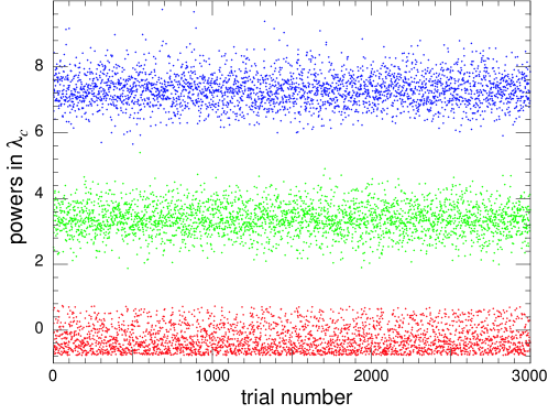
Figure 1: The powers in $\lambda_{c}$ of the positive square roots of the three eigenvalues of ${\boldsymbol{G^{(U)}}}{\boldsymbol{G^{(U)}}}^{\dagger}$ for an ensemble of 3000 Mathematica^©-randomly generated sets of ${g^{(U)}}_{ij}$ which are complex and of $\mathcal{O}(1)$.

In order to reproduce the patterns Eqs. (5.23-5.51), the $X$-charges have to fulfill, see Ref. [6],

$$X_{Q^{i}}+X_{H^{\mathcal{U}}}+X_{\overline{U^{j}}} = \left(\begin{array}[]{rrr}8&5+y&3+y\\ 7-y&4&2\\ 5-y&2&0\end{array}\right)_{\!\!ij}~{}~{},$$ (5.55)

$$X_{Q^{i}}+X_{H^{\mathcal{D}}}+X_{\overline{D^{j}}} = \left(\begin{array}[]{rrr}4+x&3+y+x&3+y+x\\ 3-y+x&2+x&2+x\\ 1-y+x&x&x\end{array}\right)_{\!\!ij},$$ (5.59)

$$X_{L^{i}}+X_{H^{\mathcal{D}}}+X_{\overline{E^{i}}} = \left(\begin{array}[]{r}4+z+x\\ 2+x\\ x\end{array}\right)_{\!\!i}\;,$$ (5.63)

with

$$x=0,1,2,3\quad{\rm if}\quad y=-7,-1,0,1\quad~{}~{}{\rm or}~{}~{}\quad x=0,1,2\quad{\rm if}\quad y=-6$$

$$\mbox{and}~{}~{}~{}~{}~{}~{}~{}z=0,1.~{}~{}~{}~{}~{}~{}~{}~{}~{}~{}~{}~{}~{}~{}~{}~{}~{}~{}~{}~{}~{}~{}~{}~{}~{}~{}~{}~{}~{}~{}$$ (5.64)

Eqs. (5.23-5.51) are in order of increasing $y$. The cases $y=-6,-7$ necessarily need supersymmetric zeros in the (1,2)- and (1,3)-entries of $\boldsymbol{G^{(U)}},\boldsymbol{G^{(D)}}$, which is why $y=-6$, $x=3$ has to be excluded. $x=3$ is our preferred value, since it requires a small value of $\tan\beta$, i.e. $\langle H^{\mathcal{U}}\rangle$ is of the same order of magnitude as $\langle H^{\mathcal{D}}\rangle$, which we find more natural than $\langle H^{\mathcal{U}}\rangle\gg\langle H^{\mathcal{D}}\rangle$. In the rest of this text we shall not deal with $y=-7,-1,1$ anymore, because $y=-6,0$ produces the best fit to the CKM matrix, not requiring any (mild) fine-tuning [as has already been stated below Eq. (5.16)]. The set of $X$-charges which is constrained by the conditions of anomaly cancellation [$S\!M$ with $U(1)_{X}$] in Section 4 and which gives rise to the phenomenology explained above is displayed in Table 1, see Ref. [6].

There is however an important no-go caveat. Ref. [63] shows that if matrices with supersymmetric zeros predict a CKM matrix which is in gross disagreement with the experimentally measured CKM matrix, then this persists even when the supersymmetric zeros are filled in, although “on first sight” the matrices in Eqs. (5.23,5.30) produce nice results. The Kähler potential for the left-handed quarks affects both the $u$- and the $d$-type mass matrices, hence the entries in the physical mass matrices are very correlated after the canonicalization. This is why during diagonalizing different terms can cancel. See also Refs. [64, 65]. Therefore the choices $y=-6$ and $-7$ actually do not reproduce the matrices in Eqs. (5.23,5.30) and hence phenomenologically uninteresting. Nonetheless, we will discuss these cases in the paper, because it is interesting to see that they are excluded by other reasons.

Should one wish to impose $SU(5)$ invariance on the $U(1)_{X}$ charge assignments, one has to work with $y=1$ and $z=\Delta^{L}_{21}=\Delta^{L}_{31}=0$. We will not be able to do so, however, as we see below, but this is consistent with our philosophy of not having an additional mass scale for grand unification. The $X$-charges in Table 1 are not compatible with invariance under flipped $SU(5)\times U(1)^{\prime}$.

$~{}\phantom{\Big{|}}X_{H^{\mathcal{D}}}$	$=$	$\frac{1}{54+9x+6z}~{}\big{[}-18+36x+18y$
		$\qquad+6x^{2}+2z^{2}+5xz-X_{L^{1}}\left(36+6x+9z\right)$
		$\qquad-\left(12+2x+2z\right)\Delta^{L}_{21}-\left(6+2x+2z\right)\Delta_{31}^{L}~{}\big{]}$
$~{}\phantom{\Big{|}}X_{H^{\mathcal{U}}}$	$=$	$-X_{H^{\mathcal{D}}}-z$
$\phantom{\Big{|}}X_{Q^{1}}$	$=$	$\frac{1}{9}\big{[}30-3X_{L^{1}}-\Delta^{L}_{21}-\Delta^{L}_{31}+3x+6y+4z\big{]}$
$~{}\phantom{\Big{|}}X_{Q^{2}}$	$=$	$X_{Q^{1}}-1-y$
$~{}\phantom{\Big{|}}X_{Q^{3}}$	$=$	$X_{Q^{1}}-3-y$
$~{}\phantom{\Big{|}}X_{\overline{D^{1}}}$	$=$	$-X_{H^{\mathcal{D}}}-X_{Q^{1}}+4+x$
$~{}\phantom{\Big{|}}X_{\overline{D^{2}}}$	$=$	$X_{\overline{D^{1}}}-1+y$
$~{}\phantom{\Big{|}}X_{\overline{D^{3}}}$	$=$	$X_{\overline{D^{1}}}-1+y$
$~{}\phantom{\Big{|}}X_{\overline{U^{1}}}$	$=$	$X_{H^{\mathcal{D}}}-X_{Q^{1}}+8+z$
$~{}\phantom{\Big{|}}X_{\overline{U^{2}}}$	$=$	$X_{\overline{U^{1}}}-3+y$
$~{}\phantom{\Big{|}}X_{\overline{U^{3}}}$	$=$	$X_{\overline{U^{1}}}-5+y$
$~{}\phantom{\Big{|}}X_{L^{2}}$	$=$	$X_{L^{1}}+\Delta^{L}_{21}$
$~{}\phantom{\Big{|}}X_{L^{3}}$	$=$	$X_{L^{1}}+\Delta^{L}_{31}$
$~{}\phantom{\Big{|}}X_{\overline{E^{1}}}$	$=$	$-X_{H^{\mathcal{D}}}{+~{}4}-X_{L^{1}}+x+z$
$~{}\phantom{\Big{|}}X_{\overline{E^{2}}}$	$=$	$-X_{H^{\mathcal{D}}}{+~{}2}-X_{L^{1}}+x-\Delta^{L}_{21}$
$~{}\phantom{\Big{|}}X_{\overline{E^{3}}}$	$=$	$-X_{H^{\mathcal{D}}}\phantom{+~{}4}-X_{L^{1}}+x-\Delta^{L}_{31}$

Table 1: The constrained $X$-charges to reproduce phenomenologically acceptable mass matrices Eqs. (5.23-5.51), with the normalization $X_{A}=-1$. $X_{L^{1}},~{}\Delta^{L}_{21},~{}\Delta^{L}_{31}$ are real numbers, for $x,y,z$ see Eq. (5.64). $SU(5)$ invariance would require $y=1$, $z=\Delta^{L}_{21}=\Delta^{L}_{31}=0$.

We now check whether Table 1 can be combined with $R_{p}$ being conserved by virtue of the $X$-charges. Eq. (3.5) is fulfilled if the $\Delta^{L}_{...}$ are integer. Eq. (3.7) is automatically fulfilled, as seen from Eqs. (5.55,5.59). With Table 1 we see

$$3X_{Q^{1}}+X_{L^{1}}=10-\mbox{$\frac{1}{3}$}(\Delta^{L}_{21}+\Delta^{L}_{31})+x+2y+\mbox{$\frac{4}{3}$}z.$$ (5.65)

Thus $3X_{Q^{1}}+X_{L^{1}}$ is integer if and only if, now working with the $\Delta^{L}_{...}$ being integers,

$$\Delta^{L}_{21}+\Delta^{L}_{31}=3\zeta+z,$$ (5.66)

and $\zeta$ is integer. With this constraint, Eq. (3.6) is fulfilled for a special choice of $X_{H^{\mathcal{D}}}$, for which we introduce the integer parameter $\Delta^{\!H}=X_{L^{1}}-X_{H^{\mathcal{D}}}-\frac{1}{2}$. So the union of Table 1 and conserved $R_{p}$ is indeed possible as given in Table 2. Note that all conclusions so far are applicable to the case of any number of right-handed neutrinos, in Table 2 however we have restricted ourselves to two right-handed neutrinos.

$~{}~{}~{}\phantom{\Big{|}}X_{H^{\mathcal{D}}}$	$=$	$\frac{1}{10~{}(6+x+z)}~{}\Big{(}12y+2x~{}(2x+11+z-2\Delta^{\!H})$
		$-z~{}(11+6\Delta^{\!H})-4~{}(6+6\Delta^{\!H}-\Delta^{L}_{31})-4~{}(6+x+z)\zeta\Big{)}~{}~{}~{}$
$~{}\phantom{\Big{|}}X_{H^{\mathcal{U}}}$	$=$	$-z-\phantom{\Big{|}}X_{H^{\mathcal{D}}}$
$~{}\phantom{\Big{|}}X_{Q^{1}}$	$=$	$\frac{1}{3}\Big{(}\frac{19}{2}-X_{H^{\mathcal{D}}}+x+2y+z-\Delta^{\!H}-\zeta\Big{)}$
$~{}\phantom{\Big{|}}X_{Q^{2}}$	$=$	$X_{Q^{1}}-1-y$
$~{}\phantom{\Big{|}}X_{Q^{3}}$	$=$	$X_{Q^{1}}-3-y$
$~{}\phantom{\Big{|}}X_{\overline{D^{1}}}$	$=$	$-X_{H^{\mathcal{D}}}-X_{Q^{1}}+4+x$
$~{}\phantom{\Big{|}}X_{\overline{D^{2}}}$	$=$	$X_{\overline{D^{1}}}-1+y$
$~{}\phantom{\Big{|}}X_{\overline{D^{3}}}$	$=$	$X_{\overline{D^{1}}}-1+y$
$~{}\phantom{\Big{|}}X_{\overline{U^{1}}}$	$=$	$X_{H^{\mathcal{D}}}-X_{Q^{1}}+8+z$
$~{}\phantom{\Big{|}}X_{\overline{U^{2}}}$	$=$	$X_{\overline{U^{1}}}-3+y$
$~{}\phantom{\Big{|}}X_{\overline{U^{3}}}$	$=$	$X_{\overline{U^{1}}}-5+y$
$~{}\phantom{\Big{|}}X_{L^{1}}$	$=$	$\frac{1}{2}+X_{H^{\mathcal{D}}}+\Delta^{\!H}$
$~{}\phantom{\Big{|}}X_{L^{2}}$	$=$	$X_{L^{1}}+z-\Delta^{L}_{31}+3\zeta$
$~{}\phantom{\Big{|}}X_{L^{3}}$	$=$	$X_{L^{1}}\phantom{+z}~{}~{}+\Delta^{L}_{31}$
$~{}\phantom{\Big{|}}X_{\overline{E^{1}}}$	$=$	$-X_{H^{\mathcal{D}}}{+~{}4}-X_{L^{1}}+x+z$
$~{}\phantom{\Big{|}}X_{\overline{E^{2}}}$	$=$	$-X_{H^{\mathcal{D}}}{+~{}2}-X_{L^{1}}+x-z+\Delta^{L}_{31}-3\zeta$
$~{}\phantom{\Big{|}}X_{\overline{E^{3}}}$	$=$	$-X_{H^{\mathcal{D}}}\phantom{+~{}4}-X_{L^{1}}+x\phantom{-z}~{}~{}-\Delta^{L}_{31}$
$~{}\phantom{\Big{|}}X_{\overline{N^{1}}}$	$=$	$\frac{1}{2}+\nu$
$~{}\phantom{\Big{|}}X_{\overline{N^{2}}}$	$=$	$\frac{1}{2}+\nu+\Delta^{\overline{N}}_{21}$

Table 2: In addition to Table 1, the automatic $R_{p}$ conservation was imposed. $\Delta^{L}_{31},~{}\zeta,~{}\Delta^{\!H},~{}\nu,~{}\Delta^{\overline{N}}_{21}$ are integers, for $x,y,z$ see Eq. (5.64). $SU(5)$ invariance would require $y=1$, $z=\Delta^{L}_{31}=\zeta=0$. We have restricted ourselves to two $\overline{N^{I}}$.

For the upcoming calculations it is useful to know that

$$X_{L^{i}}+X_{H^{\mathcal{U}}}+X_{\overline{E^{j}}}$$ (5.73)

$$= x+\left(\begin{array}[]{ccc}4+z&2&0\\ 4+z&2&0\\ 4+z&2&0\\ \end{array}\right)_{ij}+\left(\begin{array}[]{ccc}0&-\Delta^{L}_{21}&-\Delta^{L}_{31}\\ \Delta^{L}_{21}&0&\Delta^{L}_{21}-\Delta^{L}_{31}\\ \Delta^{L}_{31}&\Delta^{L}_{31}-\Delta^{L}_{21}&0\\ \end{array}\right)_{ij}$$

$$= x+\left(\begin{array}[]{ccc}4+z&2&0\\ 4+z&2&0\\ 4+z&2&0\\ \end{array}\right)_{ij}$$ (5.81)

$$\qquad+\left(\begin{array}[]{ccc}0&-z+\Delta^{L}_{31}-3\zeta&-\Delta^{L}_{31}\\ z-\Delta^{L}_{31}+3\zeta&0&z-2\Delta^{L}_{31}+3\zeta\\ \Delta^{L}_{31}&-z+2\Delta^{L}_{31}-3\zeta&0\\ \end{array}\right)_{ij}.$$

It is worth pointing out that there already exists a model in the literature which fulfills all the necessary constraints for $R_{p}$ being conserved due to the $X$-charges, namely Ref. [43] (with however three generations of right-handed neutrinos). This model is in the tradition of the papers Ref. [67] and Ref. [68]. In the former, a general analysis of $D$-flat directions and the seesaw mechanism leads to conserved $R_{p}$, in the latter, the authors worked out a concrete model. They considered three beyond-$S\!M$ $U(1)$s, two of them being generation-dependent and non-anomalous, one being generation-independent and anomalous. In Ref. [43] the before mentioned symmetries were not gauged separately but together, so that this model falls into the category considered here; in our notation, the authors work with $x=3$, $y=0$, $z=0$, $\Delta^{L}_{31}=-3$, $\zeta=-2$, $\Delta^{\!H}=1$.

6 The VEV of the Flavon; Tadpoles

Because we would like to construct a complete theory of flavor out of only two mass scales, $M_{grav}$ and $m_{3/2}$, the mass scale of the $U(1)_{X}$ breaking must be a derived scale. Indeed, the vacuum expectation value of the flavon is determined dynamically thanks to the anomalous nature of $U(1)_{X}$. We show explicitly that our $X$-charge assignments can successfully lead to an expansion parameter $\epsilon=\langle A\rangle/M_{grav}=0.171$–0.221$\simeq\lambda_{c}$ as desired phenomenologically. We, however, point out an important caveat in a class of string-derived models. We also show that tadpoles are of no concern.

In the string-embedded FN framework the expansion parameter $\epsilon$ (which will be identified with $\lambda_{c}$) has its origin solely in the Dine-Seiberg-Wen-Witten mechanism, due to which the coefficient of the Fayet-Iliopoulos term is radiatively generated. One has, see Ref. [59],

$$\xi_{X}~{}=~{}{g_{s}}^{2}~{}\frac{\mathcal{A}_{GGX}}{192\pi^{2}}~{}{M_{grav}}^{2}$$ (6.1)

(${\xi_{X}}^{tree~{}level}$ is zero in local supersymmetry, see Ref. [69]). This gives

$$\langle A\rangle~{}=~{}\sqrt{-\frac{\xi_{X}}{X_{A}}~{}},$$ (6.2)

supposing that no other fields break $U(1)_{X}$. With $X_{A}=-1$, using Eq. (4.1) to eliminate $\mathcal{A}_{GGX}$ in favor of $\mathcal{A}_{CCX}$, Eq. (4.3), Eq. (4.10) and Table 1 one finds

$$\langle A\rangle~{}=~{}\frac{g_{C}}{4\pi\sqrt{2}}\sqrt{3(6+x+z)~{}}\cdot M_{grav}.$$ (6.3)

Similar calculations with similar results have been presented in Refs. [68, 70]. Using Eq. (2.10), replacing (see Section 2)

$$M=M_{grav}$$ (6.4)

and evaluating $g_{C}[M_{GUT}=2.2\times 10^{16}\mbox{~{}GeV}]\approx 0.72$ we obtain

$$0.171\leq\epsilon\leq 0.221.$$ (6.5)

So $\epsilon=\lambda_{c}$; the best match is obtained for $x=3$, $z=1$.

However, there is a very important caveat which one should keep in mind: Eq. (6.4) together with the assumption that the dimensionless prefactors like ${g^{(...)}}_{ij}$ are of $\mathcal{O}(1)$ might well not be justified by superstring theory. In Ref. [59] it is nicely and clearly demonstrated how a prototype string theory (Ref. [71]) produces an effective supersymmetric theory with a superpotential, including the coupling constants. Translating their result to our notation we get e.g. instead of Eq. (2.2)

$$\Theta\big{[}X_{Q^{i}}+X_{H^{\mathcal{U}}}+X_{\overline{U^{j}}}\big{]}~{}\cdot~{}\Omega\big{[}X_{Q^{i}}+X_{H^{\mathcal{U}}}+X_{\overline{U^{j}}}\big{]}~{}~{}\times~{}{g}_{C}~{}~{}\sqrt{\frac{k_{C}~{}}{2}~{}}~{}~{}\mathtt{C}_{{X_{Q^{i}}+X_{H^{\mathcal{U}}}+X_{\overline{U^{j}}}}}$$

$$~{}~{}~{}~{}~{}\times~{}\mathtt{I}_{{X_{Q^{i}}+X_{H^{\mathcal{U}}}+X_{\overline{U^{j}}}}}~{}~{}\bigg{(}\frac{A}{\pi~{}M_{grav}}\bigg{)}^{{X_{Q^{i}}+X_{H^{\mathcal{U}}}+X_{\overline{U^{j}}}}}.$$ (6.6)

$\mathtt{C}_{...}$ is a $\mathcal{O}(1)$ Clebsch-Gordan coefficient and $\mathtt{I}_{...}$ a world sheet integral. For large ${X_{Q^{i}}+X_{H^{\mathcal{U}}}+X_{\overline{U^{j}}}}$ naively one would expect $\mathtt{I}_{{X_{Q^{i}}+X_{H^{\mathcal{U}}}+X_{\overline{U^{j}}}}}\sim{\mathtt{I}_{1}}^{{X_{Q^{i}}+X_{H^{\mathcal{U}}}+X_{\overline{U^{j}}}}}$ (with ${\mathtt{I}_{1}}\sim 70$), but due to destructive interference effects of the integrands actually

$$\mathtt{I}_{{X_{Q^{i}}+X_{H^{\mathcal{U}}}+X_{\overline{U^{j}}}}}\ll{70}^{{X_{Q^{i}}+X_{H^{\mathcal{U}}}+X_{\overline{U^{j}}}}},$$ (6.7)

and therefore

$${G^{(U)}}_{\!ij}~{}\ll~{}\Theta[X_{Q^{i}}+...]\cdot\Omega[X_{Q^{i}}+...]\cdot\mathtt{C}_{X_{Q^{i}}+...}~{}~{}g_{C}~{}\sqrt{\frac{k_{C}~{}}{2}}~{}~{}\bigg{(}\frac{70~{}\lambda_{c}}{\pi}\bigg{)}^{{X_{Q^{i}}+X_{H^{\mathcal{U}}}+X_{\overline{U^{j}}}}}.$$ (6.8)

This does not necessarily guarantee $\epsilon$ and the dimensionless prefactors to have the desired values. In this paper we simply assume that this is nevertheless the case. For another discussion on the calculation of fermionic mass terms in string derived models see e.g. Ref. [72].

Below the $U(1)_{X}$ breaking scale $\epsilon\cdot M_{grav}$ there are three singlets $\{A^{\prime},\overline{N^{I}}\}$, with $A^{\prime}=A-\langle A\rangle$. One must thus wonder whether these lead to tadpoles causing quadratic divergences and thus possibly destabilizing the hierarchy between the weak scale and $M_{grav}$, see Refs. [73, 74, 75, 76]. First of all, in our model $R_{p}$ is conserved before and after the breaking of $U(1)_{X}$. This prevents any $\overline{N^{I}}$-tadpole term. Second, $A^{\prime}$-tadpoles are harmless, due to the high mass of $A^{\prime}$, given by $\epsilon\cdot M_{grav}$.

7 $\boldsymbol{\mu}$-Parameter and Proton Decay

So far, we are left with the two patterns Eqs. (5.30,5.44) with $y=-6,0$, respectively, with possible choices $x=0,1,2,3~{}\big{/}~{}x=0,1,2$, respectively, and $~{}z=0,1$. In this section, we narrow down the choices further. First, the $\mu$-term is phenomenologically required to be comparable to $m_{3/2}$. This selects $z=1$. Another requirement is the adequate stability of the proton against Planck scale $D=5$ operators, which eliminates $y=-6$ and prefers larger $x$. The resulting $U(1)_{X}$ charge assignments are shown in Table 3.

In order to get a satisfactory $\mu$-term we have to rely on the GM mechanism for $\mu\propto m_{3/2}$, since $X_{H^{\mathcal{U}}}+X_{H^{\mathcal{D}}}=24$ is not possible, see Table 1. This requires $X_{H^{\mathcal{U}}}+X_{H^{\mathcal{D}}}<0$, see Eq. (2.17), hence we need $z=1.$ Thus, see Eq. (6.3),

$$\epsilon~{}=~{}0.186,~{}0.198,~{}0.210,~{}0.221~{}~{}~{}\mbox{for}~{}~{}~{}x=0,~{}1,~{}2,~{}3,~{}~{}\mbox{respectively}.$$ (7.1)

Next, we consider the proton decay constraints. We might be forced not to work with small $x$ and/or $y=-6$. This is because of the $R_{p}$-conserving but nevertheless proton destabilizing operators $\frac{\chi_{ijkl}}{M_{grav}}~{}Q^{i}Q^{j}Q^{k}L^{l}$ ($i,j,k$ must not all be the same), where

$$\chi_{ijkl}=\mathcal{O}(1)\times\epsilon^{X_{Q^{i}}+X_{Q^{j}}+X_{Q^{k}}+X_{L^{l}}}$$ (7.2)

are dimensionless coupling constants; $\overline{U}\overline{U}\overline{D}\overline{E}$ will be dealt with later in this section as well as in the second half of Subsection 8.1. With Table 2 one finds that $Q^{1}Q^{1}Q^{2}L^{i}$ has the $X$-charges

$$9+x+y+z+\left(\begin{array}[]{c}-\zeta\\ z-\Delta^{L}_{31}+2\zeta\\ \Delta^{L}_{31}-\zeta\end{array}\right)_{\!\!i}$$ (7.6)

and $Q^{2}Q^{1}Q^{2}L^{i}$ has the $X$-charges

$$~{}~{}~{}~{}~{}~{}~{}~{}~{}~{}~{}~{}~{}~{}~{}~{}~{}~{}8+x+z+\left(\begin{array}[]{c}-\zeta\\ z-\Delta^{L}_{31}+2\zeta\\ \Delta^{L}_{31}-\zeta\end{array}\right)_{\!\!i}.$$ (7.10)

In comparison, operators involving third-generation quarks are enhanced due to lower $X$-charges. But their contributions to proton decay are suppressed by the entries of the matrices that transform from the weak base into the mass base, see Ref. [8].

For both equations above one sees that suppressing one of the three operators by choosing an appropriate $\zeta$ and/or $\Delta^{L}_{31}$ makes one or both of the others less suppressed. The “average $X$-charges” of $Q^{1}Q^{1}Q^{2}L^{i}$ ($\sum_{i}X_{Q^{1}Q^{1}Q^{2}L^{i}}/3$) and $Q^{2}Q^{1}Q^{2}L^{i}$ are $9+x+y+\frac{4z}{3}$ and $8+x+\frac{4z}{3}$, which are not very high [note that already in Ref. [46] it was anticipated that e.g. $z=1$ (our notation) gives a more stable proton than $z=0$]. Thus already now we can see that the model could get into trouble due to proton decay if we work with the wrong choices for $x,y,\zeta,\Delta^{L}_{31}$. For a first crude estimate we use

$$\chi~{}\leq~{}\frac{\frac{M_{grav}}{\phantom{\big{|}}\mbox{{\small{1 GeV}}}}}{\sqrt{~{}2\times 10^{17\pm 0.7}\times\frac{\tau}{\mbox{\small years}}~{}}}~{}\times~{}\frac{m_{squark}}{\mbox{1 TeV}}.$$ (7.11)

$\tau$ is the upper bound on the proton lifetime, about $5\times 10^{33}~{}$years for the $p\rightarrow\pi^{0}+\overline{e}$ mode, see e.g. Refs. [20, 21]. The coefficient $2\times 10^{17\pm 0.7}$ is extracted from Ref. [81]. Being as strict as possible one finds

$$\chi~{}\leq~{}3\times 10^{-8}~{}\times~{}\frac{m_{squark}}{\mbox{{1 TeV}}}.$$ (7.12)

Now $3\times 10^{-8}\sim 0.22^{11}$. Thus comparing the exponent with the “average $X$-charges” it becomes apparent that $y=-6$ is not an option, we are thus left with $y=0$. Furthermore, one sees that $x=3$ (our preferred value; not possible with $y=-6$) is the safest choice to make, but we have not fixed the parameters of our model enough yet to say that $x=0,1,2$ are not viable.

For a more quantitative investigation we will in the next Section rely on Ref. [46]’s treatment of the so called “best-fit” scenario, taking into account both $QQQL$ and $\overline{U}\overline{U}\overline{D}\overline{E}$ (note that $QQQH^{\mathcal{D}}$ violates $R_{p}$ and thus is forbidden by the $X$-charges). Translated to the notation of Table 2, they state that the $X$-charges have to fulfill (with $m_{squark}=$1 TeV, $y=0$, $z=1$ )

$$\mathcal{O}(1)\times\epsilon^{x+10+\Delta^{L}_{31}-\zeta} < 4\times 10^{-8},$$

$$\mathcal{O}(1)\times\epsilon^{x+10-\Delta^{L}_{31}+\zeta}~{}\frac{\langle H^{\mathcal{U}}\rangle}{\langle H^{\mathcal{D}}\rangle} < 1\times 10^{-7},$$ (7.13)

in order not to be in conflict with experiment. With $m_{t}/m_{b}$ at high energies being $\sim 100$ (see Ref. [46]) we get from $m_{b}\sim\langle H^{\mathcal{D}}\rangle\epsilon^{x}$, $m_{t}\sim\langle H^{\mathcal{U}}\rangle$ that $100~{}\epsilon^{x}\sim{\langle H^{\mathcal{U}}\rangle}/{\langle H^{\mathcal{D}}\rangle}$. Thus

$$\mathcal{O}(1)\times\epsilon^{x+10+\Delta^{L}_{31}-\zeta} < 4\times 10^{-8},$$

$$\mathcal{O}(1)\times\epsilon^{2x+10-\Delta^{L}_{31}+\zeta} < 1\times 10^{-9}.$$ (7.14)

Note that our model with $y=0$, $z=1$, $\Delta^{L}_{21}=\Delta^{L}_{31}=-1$, and $\zeta=-1$ is a special case of the “best fit” model in Ref. [46] with $m=1$ in their notation, while they took $X_{L^{3}}$ as a free parameter, because they do not impose the anomaly cancellation conditions nor conserved $R_{p}$ as a consequence of the $U(1)_{X}$ symmetry. A more thorough study of proton decay due to higher-dimensional operators and $R_{p}$-conserving $X$-charges will be presented in Ref. [82].

$~{}~{}~{}\phantom{\Big{|}}X_{H^{\mathcal{D}}}$	$=$	$\frac{1}{10~{}(7+x)}~{}\Big{(}2x~{}(2x+12-2\Delta^{\!H})$
		$-(11+6\Delta^{\!H})-4~{}(6+6\Delta^{\!H}-\Delta^{L}_{31})-4~{}(7+x)\zeta\Big{)}~{}~{}~{}$
$~{}\phantom{\Big{|}}X_{H^{\mathcal{U}}}$	$=$	$-1-\phantom{\Big{|}}X_{H^{\mathcal{D}}}$
$~{}\phantom{\Big{|}}X_{Q^{1}}$	$=$	$\frac{1}{3}\Big{(}\frac{21}{2}-X_{H^{\mathcal{D}}}+x-\Delta^{\!H}-\zeta\Big{)}$
$~{}\phantom{\Big{|}}X_{Q^{2}}$	$=$	$X_{Q^{1}}-1$
$~{}\phantom{\Big{|}}X_{Q^{3}}$	$=$	$X_{Q^{1}}-3$
$~{}\phantom{\Big{|}}X_{\overline{D^{1}}}$	$=$	$-X_{H^{\mathcal{D}}}-X_{Q^{1}}+4+x$
$~{}\phantom{\Big{|}}X_{\overline{D^{2}}}$	$=$	$X_{\overline{D^{1}}}-1$
$~{}\phantom{\Big{|}}X_{\overline{D^{3}}}$	$=$	$X_{\overline{D^{1}}}-1$
$~{}\phantom{\Big{|}}X_{\overline{U^{1}}}$	$=$	$X_{H^{\mathcal{D}}}-X_{Q^{1}}+9$
$~{}\phantom{\Big{|}}X_{\overline{U^{2}}}$	$=$	$X_{\overline{U^{1}}}-3$
$~{}\phantom{\Big{|}}X_{\overline{U^{3}}}$	$=$	$X_{\overline{U^{1}}}-5$
$~{}\phantom{\Big{|}}X_{L^{1}}$	$=$	$\frac{1}{2}+X_{H^{\mathcal{D}}}+\Delta^{\!H}$
$~{}\phantom{\Big{|}}X_{L^{2}}$	$=$	$X_{L^{1}}+1-\Delta^{L}_{31}+3\zeta$
$~{}\phantom{\Big{|}}X_{L^{3}}$	$=$	$X_{L^{1}}\phantom{+1}~{}~{}+\Delta^{L}_{31}$
$~{}\phantom{\Big{|}}X_{\overline{E^{1}}}$	$=$	$-X_{H^{\mathcal{D}}}{+~{}5}-X_{L^{1}}+x$
$~{}\phantom{\Big{|}}X_{\overline{E^{2}}}$	$=$	$-X_{H^{\mathcal{D}}}{+~{}1}-X_{L^{1}}+x+\Delta^{L}_{31}-3\zeta$
$~{}\phantom{\Big{|}}X_{\overline{E^{3}}}$	$=$	$-X_{H^{\mathcal{D}}}\phantom{+~{}4}-X_{L^{1}}+x~{}~{}-\Delta^{L}_{31}$
$~{}\phantom{\Big{|}}X_{\overline{N^{1}}}$	$=$	$\frac{1}{2}+\nu$
$~{}\phantom{\Big{|}}X_{\overline{N^{2}}}$	$=$	$\frac{1}{2}+\nu+\Delta^{\overline{N}}_{21}$

Table 3: In addition to Table 2, the constraints from the $\mu$-parameter $z=1$ and proton decay $y=0$ are imposed. Furthermore, proton decay prefers $x=2,3$ over $x=0,1$. $\Delta^{L}_{31},~{}\zeta,~{}\Delta^{\!H},~{}\nu,~{}\Delta^{\overline{N}}_{21}$ are integers.

8 Neutrino Phenomenology

Our study of the neutrino sector is far more constrained than most models in the literature. This is because there is no GUT scale, which is a factor of $\sim 100$ lower than $M_{grav}$, to suppress the mass scale of the Majorana mass terms $\sim 10^{15}$ GeV, or equivalently, boost the light neutrino masses to the required orders of magnitude. In typical seesaw models (see Refs. [77, 78, 79, 80]), it is achieved using an extra symmetry, such as gauged $U(1)_{B-L}$. However, in our scenario there are no additional symmetries beyond the $M\!S\!S\!M$ gauge groups and $U(1)_{X}$ nor additional mass scales beyond $M_{grav}$ and $m_{3/2}$; therefore the mass scales of right-handed neutrinos originate from $M_{grav}$, suppressed by powers of $\epsilon$. As our model contains only two right-handed neutrinos, the mass of the lightest neutrino is zero. The successful neutrino phenomenology together with proton decay constraints determine the $U(1)_{X}$ charge assignments down to four choices, see Tables 6-9.

Because this discussion is rather long, we have divided this section into the following subsections. In Section 8.1, we review our phenomenological understanding of neutrino mixings and discuss their implications on $U(1)_{X}$ charge assignments. Phenomenology requires $\zeta=\Delta_{31}^{L}=-1$ as well as $z=1$, thus justifying the GM mechanism for the $\mu$-parameter from a completely different reasoning. The resulting charge assignments are shown in Table 4. Section 8.2 is the corresponding discussion of neutrino mass eigenvalues. Here we encounter different possibilities depending on whether $LL$, $LR$ and $RR$ entries of the neutrino mass matrices are induced by the GM mechanism, schematically shown in Table 5: Section 8.2.1 discusses cases 1.), 2.), and 3.), while Section 8.2.2 discusses cases 4.), 5.), and 6.). We find successful solutions to cases 2.) and 6.). The former case is similar to the standard seesaw scenario, and $U(1)_{X}$ charge assignments are shown in Tables 6 and 7. The latter case has the right-handed neutrino masses from the GM mechanism and hence they are present below the electroweak scale. The $U(1)_{X}$ charge assignments are shown in Tables 8 and 9.

8.1 Neutrino Mixing

If there are no filled up supersymmetric zeros in $\boldsymbol{G^{(U)}}$ and $\boldsymbol{G^{(D)}}$, then, see Ref. [2],

$${V^{\!C\!K\!M}}_{ij}\sim\epsilon^{|X_{Q^{i}}-X_{Q^{j}}|}.$$ (8.1)

Analogously, if there are no filled up supersymmetric zeros in the mass matrices in the leptonic sector, one has

$${U^{\!M\!N\!S}}_{ij}\sim\epsilon^{|X_{L^{i}}-X_{L^{j}}|},$$ (8.2)

i.e. a symmetric (with respect to the $\epsilon$-suppression) Maki-Nagakawa-Sakata (MNS) matrix (see Ref. [83]). Phenomenology suggests, see e.g. Ref. [84] (using Refs. [89, 85])

$${\boldsymbol{U^{\!M\!N\!S}}}~{}\sim~{}\left(\begin{array}[]{lll}1&\epsilon&\epsilon\\ \epsilon&1&1\\ \epsilon&1&1\end{array}\right),$$ (8.6)

with possibly higher exponents of $\epsilon$ in the (1,3)-element. Comparing with Eq. (8.2) gives

$$|X_{L^{1}}-X_{L^{2}}|=|X_{L^{1}}-X_{L^{3}}|=1,~{}~{}~{}|X_{L^{2}}-X_{L^{3}}|=0,$$ (8.7)

so that

$$\Delta^{L}_{21}=\Delta^{L}_{31}=\pm 1.$$ (8.8)

Combining this with Eq. (5.66) gives

$$\zeta=\frac{\pm 2-z}{3}.$$ (8.9)

Since $\zeta$ has to be integer, one is left with

$$\zeta=\Delta^{L}_{31}=-1~{}~{}~{}\mbox{and}~{}~{}~{}z=1.$$ (8.10)

It is interesting to notice that the MNS phenomenology combined with the requirement that there are no filled up superymmetric zeros and guaranteeing $R_{p}$ the way advocated here predicts $z=1$, i.e. the necessity to have the $\mu$-term generated via GM! We also looked at the more general case with the possibility of supersymmetric zeros in $\boldsymbol{G^{(N)}}$ and $\boldsymbol{G^{(E)}}$, not leading to a substantially different result. For completeness the calculations generalizing the lower case of the lower left-hand corner of Table 5 are given in Appendix C. Plugging Eq. (8.10) and $y=0$ into Table 2 gives Table 4. The only non-neutrino parameters left unfixed are $x$ and $\Delta^{\!H}$.

From Eq. (8.10) one can observe furthermore that there are no supersymmetric zeros for the superfield operators $QQQL$ and $\overline{U}\overline{U}\overline{D}\overline{E}$ so that the canonicalization of the Kähler potential does not affect the order of $\epsilon$-suppression. With the results of Ref. [86], also translated to the mass matrices of charged leptons and light neutrinos we find that the powers of $\epsilon$ for $QQQL$ and $\overline{U}\overline{U}\overline{D}\overline{E}$ are again not changed when going to the mass basis. With Eq. (8.10) and

$$0.186^{10}\approx 5\times 10^{-8}, 0.186^{10}\approx 5\times 10^{-8},$$

$$0.198^{11}\approx 2\times 10^{-8}, 0.198^{12}\approx 4\times 10^{-9},$$

$$0.210^{12}\approx 7\times 10^{-9}, 0.210^{14}\approx 3\times 10^{-10},$$

$$0.221^{13}\approx 3\times 10^{-9}, 0.221^{16}\approx 3\times 10^{-11}$$ (8.11)

together with Eq. (7), one finds that the cases with $x=0,1$ are ruled out, only $x=2,3$ are viable, while $x=3$ is allowed even for $m_{squark}=100$ GeV.

Will we be able to have an $X$-charge assignment such that no hidden sector fields are needed in order to cancel the anomalies of $U(1)_{X}$ with itself and gravity? Table 1 and Eq. (4.7) give

$$\mathcal{A}_{GGX}=59-3X_{H^{\mathcal{D}}}+3X_{L^{1}}+12x+8z+\Delta^{L}_{21}+\Delta^{L}_{31}+\sum_{I}X_{\overline{N^{I}}}+\mathcal{A}_{GGX}^{hidden~{}sector},$$ (8.12)

focusing on our $R_{p}$-conserving scenario one obtains

$$\mathcal{A}_{GGX}=\frac{121}{2}+12x+9z+3\Delta^{\!H}+3\zeta+\sum_{I}X_{\overline{N^{I}}}+\mathcal{A}_{GGX}^{hidden~{}sector}.$$ (8.13)

With Eq. (8.10) and assuming no $X$-charged hidden fields we get

$$\mathcal{A}_{GGX}=66+\mbox{$\frac{1}{2}$}+12x+3\Delta^{\!H}+\sum_{I}X_{\overline{N^{I}}}.$$ (8.14)

With Eq. (4.1) and $x=3$ (and hence $\mathcal{A}_{CCX}=30/2$), one finds that ${360}/{k_{C}}$ has to be a half-odd-integer number, which is only given for $k_{C}=16,48,80,144,240,720$, resulting in $~{}3\Delta^{\!H}+\sum_{I}X_{\overline{N^{I}}}=-80,-95,-98,-100,-101,-102$,  respectively. Analogously for $x=2$ (and hence $\mathcal{A}_{CCX}=27/2$), we obtain $k_{C}=8,24,72,216,648$ and $~{}3\Delta^{\!H}+\sum_{I}X_{\overline{N^{I}}}=-50,-77,-86,-89,-90$,  respectively. We consider this to be highly unlikely (confirmed in the next Subsections), since it requires extremely large $X$-charges. Moreover, such charge assignments would require the neutrino Dirac mass matrix to be generated by the GM mechanism and hence the neutrino masses come out too small (see the next subsection). So to have only $M\!S\!S\!M$ superfields and $\{A,\overline{N^{I}}\}$ to be $X$-charged is not possible. The rest of the goals mentioned in Section 2 will be achieved however.

It should be mentioned that phenomenology might also suggest the so called anarchical scenario, see Refs. [87, 44, 88], i.e. instead of Eq. (8.6) one has

$${\boldsymbol{U^{\!M\!N\!S}}}~{}\sim~{}\left(\begin{array}[]{lll}1&1&1\\ 1&1&1\\ 1&1&1\end{array}\right).$$ (8.18)

However, this is not compatible with $z=1$ in combination with Eq. (5.66).

$~{}~{}~{}\phantom{\Big{|}}X_{H^{\mathcal{D}}}$	$=$	$\frac{2}{5}-\frac{39-4\,x\,\left(6+x-{\Delta^{\!H}}\right)+30\,{\Delta^{\!H}}}{10\,\left(7+x\right)}$
$~{}\phantom{\Big{|}}X_{H^{\mathcal{U}}}$	$=$	$-1-\phantom{\Big{|}}X_{H^{\mathcal{D}}}$
$~{}\phantom{\Big{|}}X_{Q^{1}}$	$=$	$\frac{1}{3}\Big{(}\frac{23}{2}-X_{H^{\mathcal{D}}}+x-\Delta^{\!H}\Big{)}$
$~{}\phantom{\Big{|}}X_{Q^{2}}$	$=$	$X_{Q^{1}}-1$
$~{}\phantom{\Big{|}}X_{Q^{3}}$	$=$	$X_{Q^{1}}-3$
$~{}\phantom{\Big{|}}X_{\overline{D^{1}}}$	$=$	$-X_{H^{\mathcal{D}}}-X_{Q^{1}}+4+x$
$~{}\phantom{\Big{|}}X_{\overline{D^{2}}}$	$=$	$X_{\overline{D^{1}}}-1$
$~{}\phantom{\Big{|}}X_{\overline{D^{3}}}$	$=$	$X_{\overline{D^{1}}}-1$
$~{}\phantom{\Big{|}}X_{\overline{U^{1}}}$	$=$	$X_{H^{\mathcal{D}}}-X_{Q^{1}}+9$
$~{}\phantom{\Big{|}}X_{\overline{U^{2}}}$	$=$	$X_{\overline{U^{1}}}-3$
$~{}\phantom{\Big{|}}X_{\overline{U^{3}}}$	$=$	$X_{\overline{U^{1}}}-5$
$~{}\phantom{\Big{|}}X_{L^{1}}$	$=$	$\frac{1}{2}+X_{H^{\mathcal{D}}}+\Delta^{\!H}$
$~{}\phantom{\Big{|}}X_{L^{2}}$	$=$	$X_{L^{1}}-1$
$~{}\phantom{\Big{|}}X_{L^{3}}$	$=$	$X_{L^{1}}-1$
$~{}\phantom{\Big{|}}X_{\overline{E^{1}}}$	$=$	$-X_{H^{\mathcal{D}}}{+~{}5}-X_{L^{1}}+x$
$~{}\phantom{\Big{|}}X_{\overline{E^{2}}}$	$=$	$-X_{H^{\mathcal{D}}}{+~{}3}-X_{L^{1}}+x$
$~{}\phantom{\Big{|}}X_{\overline{E^{3}}}$	$=$	$-X_{H^{\mathcal{D}}}{+~{}1}-X_{L^{1}}+x$
$~{}\phantom{\Big{|}}X_{\overline{N^{1}}}$	$=$	$\frac{1}{2}+\nu$
$~{}\phantom{\Big{|}}X_{\overline{N^{2}}}$	$=$	$\frac{1}{2}+\nu+\Delta^{\overline{N}}_{21}$

Table 4: In addition to Table 3, we required successful neutrino mixings, i.e., $\Delta^{L}_{31}=\zeta=-1$. The remaining parameters $\Delta^{\!H},~{}\nu,~{}\Delta^{\overline{N}}_{21}$ are integers, while $x=2$ or 3 to satisfy proton decay constraints.

8.2 Neutrino Masses

After looking at the mixing, let us now investigate the relationship between the neutrino mass spectrum and the $X$-charges. For future reference we here state the experimental status, allowing for three possible neutrino mass solutions, see e.g. Ref. [19] and references therein:

• “hierarchical”($m_{\nu^{3}}$ is much larger than $m_{\nu^{2}}$, which is much larger than $m_{\nu^{1}}$),

  $${m_{\nu^{2}}}^{2}-{m_{\nu^{1}}}^{2}\phantom{-} \sim \phantom{-}7\times 10^{-5}~{}\mbox{eV}^{2},$$

  $${m_{\nu^{3}}}^{2}-{m_{\nu^{2}}}^{2}\phantom{-} \sim \phantom{-}3\times 10^{-3}~{}\mbox{eV}^{2},$$ (8.19)

• “inverse hierarchical”($m_{\nu^{2}}$ is minutely larger than $m_{\nu^{1}}$, which is much larger than $m_{\nu^{3}}$; this is not possible in our scenario),

  $${m_{\nu^{2}}}^{2}-{m_{\nu^{1}}}^{2}\phantom{-} \sim \phantom{-}7\times 10^{-5}~{}\mbox{eV}^{2},$$

  $${m_{\nu^{3}}}^{2}-{m_{\nu^{2}}}^{2}\phantom{-} \sim -3\times 10^{-3}~{}\mbox{eV}^{2},$$ (8.20)

• “quasi-degenerate” (all $m_{\nu}$ are almost identical; this is not possible in our scenario).

The scenario sketched so far (with $x=2,3$, $y=0$, $z=1$, $\zeta=-1$, $\Delta^{L}_{31}=-1$) generates a superpotential (neglecting the tiny contributions of the GM mechanism to $\boldsymbol{G^{(U,D,E)}}$) with [for $\boldsymbol{G^{(E)}}$ see Eq. (5.73)]

$$\mathcal{W}^{M\!S\!S\!M}~{} = ~{}{g^{(U)}}_{\!ij}~{}\left(\begin{array}[]{lll}\epsilon^{8}&\epsilon^{5}&\epsilon^{3}\\ \epsilon^{7}&\epsilon^{4}&\epsilon^{2}\\ \epsilon^{5}&\epsilon^{2}&1\end{array}\!\!\right)_{\!ij}~{}Q^{i}~{}{H^{\mathcal{U}}}~{}\overline{U^{j}}~{}+~{}m_{3/2}~{}~{}\widetilde{g^{(\mu)}}~{}~{}\epsilon~{}{H^{\mathcal{D}}}~{}{H^{\mathcal{U}}}$$ (8.32)

$$+~{}{g^{(D)}}_{\!ij}~{}\epsilon^{{2~{}\mbox{\scriptsize or}~{}3}}~{}\left(\begin{array}[]{lll}\epsilon^{4}&\epsilon^{3}&\epsilon^{3}\\ \epsilon^{3}&\epsilon^{2}&\epsilon^{2}\\ \epsilon&1&1\end{array}\right)_{\!ij}~{}Q^{i}~{}{H^{\mathcal{D}}}~{}\overline{D^{j}}~{}$$

$$+~{}{g^{(E)}}_{\!ij}~{}\epsilon^{2~{}\mbox{\scriptsize or}~{}3}~{}\left(\begin{array}[]{lll}\epsilon^{5}&\epsilon^{3}&\epsilon\\ \epsilon^{4}&\epsilon^{2}&1\\ \epsilon^{4}&\epsilon^{2}&1\end{array}\right)_{\!ij}~{}L^{i}~{}{H^{\mathcal{D}}}~{}\overline{E^{j}},$$

and

$$\mathcal{W}^{(\nu)} = \frac{1}{2}~{}\Big{(}\Theta[X_{\overline{N^{I}}}+X_{\overline{N^{J}}}]~{}~{}M_{grav}~{}~{}\gamma_{\!IJ}~{}~{}\epsilon^{X_{\overline{N^{I}}}+X_{\overline{N^{J}}}}$$ (8.33)

$$\qquad+~{}m_{3/2}\cdot\widetilde{\gamma}_{\!IJ}~{}~{}\epsilon^{|X_{\overline{N^{I}}}+X_{\overline{N^{J}}}|}\Big{)}~{}~{}\overline{N^{I}}~{}~{}\overline{N^{J}}~{}~{}$$

$$+~{}~{}\Big{(}\Theta[X_{L^{i}}+X_{H^{\mathcal{U}}}+X_{\overline{N^{J}}}]~{}~{}{g^{(N)}}_{\!iJ}~{}~{}\epsilon^{X_{L^{i}}+X_{H^{\mathcal{U}}}+X_{\overline{N^{J}}}}~{}~{}$$

$$\qquad+~{}~{}\frac{m_{3/2}}{M_{grav}}\cdot{\widetilde{g^{(N)}}}_{\!iJ}~{}~{}\epsilon^{|X_{L^{i}}+X_{H^{\mathcal{U}}}+X_{\overline{N^{J}}}|}\Big{)}~{}~{}{L^{i}}~{}~{}{H^{\mathcal{U}}}~{}~{}\overline{N^{J}}$$

$$+~{}~{}\frac{1}{2}~{}\Big{(}\Theta[X_{L^{i}}+X_{H^{\mathcal{U}}}+X_{L^{j}}+X_{H^{\mathcal{U}}}]~{}~{}\frac{{\psi_{\!ij}}}{M_{grav}}~{}~{}\epsilon^{X_{L^{i}}+X_{H^{\mathcal{U}}}+X_{L^{j}}+X_{H^{\mathcal{U}}}}~{}~{}$$

$$\qquad+~{}~{}\frac{m_{3/2}}{M_{grav}}\cdot\frac{{\widetilde{\psi}}_{\!ij}}{M_{grav}}~{}~{}\epsilon^{|X_{L^{i}}+X_{H^{\mathcal{U}}}+X_{L^{j}}+X_{H^{\mathcal{U}}}|}\Big{)}~{}~{}{L^{i}}~{}~{}{H^{\mathcal{U}}}~{}~{}{L^{j}}~{}~{}{H^{\mathcal{U}}};~{}~{}~{}~{}~{}~{}~{}$$

summation over repeated indices is implied. The two equations above do not contain any factors of $\Omega[...]$, because by construction all $R_{p}$-conserving terms have integer $X$-charge. We will in turn investigate the different possibilities for generating the mass terms, as given in Table 5. With $y=0$ all exponents in $\boldsymbol{G^{(U,D,E)}}$ are positive. From this one may feel inspired to assume either that all exponents in the mass terms of the neutrinos are positive (the case in the lower right-hand corner of Table 5), or (less restrictive) simply that for a given array of neutrino coupling constants all exponents are either negative or positive.

 
$X_{L^{i}}+X_{H^{\mathcal{U}}}<0$ $X_{L^{i}}+X_{H^{\mathcal{U}}}>0$ 5.) $X_{L^{i}}+X_{H^{\mathcal{U}}}<-X_{\overline{N^{I}}}$ $\boldsymbol{M_{LL}^{Maj}}$: FN 4.) $\boldsymbol{M_{LR}^{Dirac}}$: GM $X_{\overline{N^{I}}}$ $\boldsymbol{M_{LL}^{Maj}}$: GM $\boldsymbol{M_{RR}^{Maj}}$: GM $<0$ $\boldsymbol{M_{LR}^{Dirac}}$: GM 6.) $X_{L^{i}}+X_{H^{\mathcal{U}}}\geq-X_{\overline{N^{I}}}$ $\boldsymbol{M_{RR}^{Maj}}$: GM $\boldsymbol{M_{LL}^{Maj}}$: FN $\boldsymbol{M_{LR}^{Dirac}}$: FN $\boldsymbol{M_{RR}^{Maj}}$: GM 3.) $X_{\overline{N^{I}}}<-X_{L^{i}}-X_{H^{\mathcal{U}}}$ $\boldsymbol{M_{LL}^{Maj}}$: GM $\boldsymbol{M_{LR}^{Dirac}}$: GM 1.) $X_{\overline{N^{I}}}$ $\boldsymbol{M_{RR}^{Maj}}$: FN $\boldsymbol{M_{LL}^{Maj}}$: FN $>0$ 2.) $X_{\overline{N^{I}}}\geq-X_{L^{i}}-X_{H^{\mathcal{U}}}$ $\boldsymbol{M_{LR}^{Dirac}}$: FN $\boldsymbol{M_{LL}^{Maj}}$: GM $\boldsymbol{M_{RR}^{Maj}}$: FN $\boldsymbol{M_{LR}^{Dirac}}$: FN $\boldsymbol{M_{RR}^{Maj}}$: FN

Table 5: The Majorana mass of the left-handed neutrinos is denoted by $\boldsymbol{M_{LL}^{Maj}}$, the one for the right-handed neutrinos is given by $\boldsymbol{M_{RR}^{Maj}}$, and the Dirac mass is $\boldsymbol{M_{LR}^{Dirac}}.$ We work with two right-handed neutrinos.

Are the cases sketched in Table 5 Majorana or pseudo Dirac neutrinos? One has pseudo Dirac neutrinos if $\boldsymbol{M_{LR}^{Dirac}}\gg\boldsymbol{M_{LL}^{Maj}},\boldsymbol{M_{RR}^{Maj}}$. We will investigate case by case (starting in the lower right-hand corner, proceeding anticlockwise) whether this condition can be met when $\boldsymbol{M_{LR}^{Dirac}}$ is generated via the FN mechanism, since $\boldsymbol{M_{LR}^{Dirac}}$ generated by the GM mechanism produces neutrino masses which are too small, one has that $[{M_{LR}^{Dirac}}]_{ij}\approx\epsilon^{|X_{L^{i}}+X_{\overline{N^{j}}}+X_{H^{\cal U}}|}\,\langle H^{\mathcal{U}}\rangle~{}m_{3/2}/M_{grav}\leq 10^{-5}$ eV.

8.2.1 Positive $\boldsymbol{X_{\overline{N^{I}}}}$

First we will take the $X$-charges of all right-handed neutrino superfields to be positive. This ensures that the scalar component of $A$ acquires a VEV, since its $X$-charge is negative and $\xi_{X}$ is positive. This way the $D_{\!X}$-term does not acquire a VEV and supersymmetry is not broken by the DSWW mechanism, see Ref. [14, 15, 16, 17], at a much too high energy scale.

Of course, guaranteeing a VEV for $A$ does not automatically guarantee that the scalar components of the right-handed neutrino superfields do not get VEVs – this we simply have to postulate, in order to conserve $R_{p}$ and to have only one flavon field.

1.) We now consider the case in the lower right corner of Table 5. All $\Theta[...]$ can be dropped:

$$\mathcal{W}^{(\nu)} = M_{grav}~{}~{}\frac{\gamma_{\!IJ}}{2}~{}~{}\epsilon^{X_{\overline{N^{I}}}+X_{\overline{N^{J}}}}~{}~{}\overline{N^{I}}~{}~{}\overline{N^{J}}~{}~{}+~{}~{}{g^{(N)}}_{\!iJ}~{}~{}\epsilon^{X_{L^{i}}+X_{H^{\mathcal{U}}}+X_{\overline{N^{J}}}}~{}~{}{L^{i}}~{}~{}{H^{\mathcal{U}}}~{}~{}\overline{N^{J}}$$ (8.34)

$$+~{}~{}\frac{{\psi_{\!ij}}}{2~{}M_{grav}}~{}~{}\epsilon^{X_{L^{i}}+X_{H^{\mathcal{U}}}+X_{L^{j}}+X_{H^{\mathcal{U}}}}~{}~{}{L^{i}}~{}~{}{H^{\mathcal{U}}}~{}~{}{L^{j}}~{}~{}{H^{\mathcal{U}}},~{}~{}~{}~{}~{}~{}~{}$$

for short (dropping all generational indices)

$$\mathcal{W}^{(\nu)} = M_{grav}~{}~{}\overline{\boldsymbol{N}}^{T}~{}~{}\frac{\boldsymbol{\Gamma}}{2}~{}~{}\overline{\boldsymbol{N}}~{}~{}+~{}~{}\boldsymbol{L}^{T}~{}~{}\boldsymbol{G^{(N)}}~{}~{}{H^{\mathcal{U}}}~{}~{}\overline{\boldsymbol{N}}~{}~{}$$ (8.35)

$$~{}~{}~{}~{}~{}~{}+~{}~{}\frac{1}{M_{grav}}~{}~{}\boldsymbol{L}^{T}~{}~{}\frac{\boldsymbol{\Psi}}{2}~{}~{}\boldsymbol{L}~{}~{}{H^{\mathcal{U}}}~{}~{}{H^{\mathcal{U}}}.$$

We get a Lagrangian with ($\boldsymbol{n_{L/R}}$ are left/right-handed neutrinos in the interaction basis)

$$\mathcal{L}\supset\langle H^{\mathcal{U}}\rangle~{}\boldsymbol{n_{L}}^{T}~{}\boldsymbol{G^{(N)}}~{}\overline{\boldsymbol{n_{R}}}~{}+~{}M_{grav}~{}\overline{\boldsymbol{n_{R}}}^{T}~{}\frac{\boldsymbol{\Gamma}}{2}~{}\overline{\boldsymbol{n_{R}}}~{}+~{}\frac{\langle H^{\mathcal{U}}\rangle^{2}}{M_{grav}}~{}\boldsymbol{n_{L}}^{T}~{}\frac{\boldsymbol{\Psi}}{2}~{}\boldsymbol{n_{L}},$$ (8.36)

which equals

$$\mathcal{L} \supset \frac{1}{2}~{}\left(\boldsymbol{n_{L}}^{T},~{}~{}\overline{\boldsymbol{n_{R}}}^{T}\right)\cdot\left(\begin{array}[]{ccc}{\langle H^{\mathcal{U}}\rangle^{2}}~{}\frac{\boldsymbol{\Psi}}{M_{grav}}&{}\hfil&{\langle H^{\mathcal{U}}\rangle}~{}\boldsymbol{G^{(N)}}\\ {}\hfil&{}\hfil&{}\hfil\\ \langle H^{\mathcal{U}}\rangle~{}\boldsymbol{G^{(N)}}^{T}&{}\hfil&M_{grav}~{}~{}\boldsymbol{\Gamma}\end{array}\right)\cdot\left(\begin{array}[]{c}\boldsymbol{n_{L}}\\ {}\hfil\\ \overline{\boldsymbol{n_{R}}}\end{array}\right).~{}~{}~{}~{}~{}~{}~{}~{}$$ (8.43)

For the Majorana case, the masses of the light neutrinos are given by the positive square roots of the eigenvalues of $~{}~{}\big{(}\langle H^{\mathcal{U}}\rangle^{2}/M_{grav}\big{)}^{2}~{}\boldsymbol{\mathcal{G}^{(\nu)}}\boldsymbol{\mathcal{G}^{(\nu)}}^{\dagger}$, with

$$\boldsymbol{\mathcal{G}^{(\nu)}}\equiv\boldsymbol{\Psi}-\boldsymbol{G^{(N)}}~{}\boldsymbol{\Gamma}^{-1}~{}\boldsymbol{G^{(N)}}^{T}$$ (8.44)

(for a derivation see Appendix A). Note that this statement is not the same as saying “the masses of the light neutrinos are given by the absolute values of the eigenvalues of $\langle H^{\mathcal{U}}\rangle^{2}/M_{grav}~{}\boldsymbol{\mathcal{G}^{(\nu)}}$”. However, since the entries of $\boldsymbol{\mathcal{G}^{(\nu)}}$ are hierarchically $\epsilon$-suppressed it is a good approximation, for a demonstration see Ref. [6]; we shall assume here that this approximation has been made. One has

$$[{{\boldsymbol{\Gamma}}}^{-1}]_{IJ}~{}=~{}[\boldsymbol{{\gamma}}^{-1}]_{IJ}~{}~{}\epsilon^{-X_{\overline{N^{I}}}-X_{\overline{N^{J}}}}.$$ (8.45)

It follows that

$${\mathcal{G}^{(\nu)}}_{ij}~{}=~{}\epsilon^{X_{L^{i}}+X_{L^{j}}+2X_{H^{\mathcal{U}}}}~{}~{}\Big{(}\psi_{ij}~{}-~{}\sum_{K,L}~{}~{}{g^{(N)}}_{iK}~{}~{}[\boldsymbol{{\gamma}}^{-1}]_{KL}~{}~{}{g^{(N)}}_{jL}\Big{)}.$$ (8.46)

Note that this result also holds when there are supersymmetric zeros (as long as $\boldsymbol{\Gamma}$ is invertible), one just has to replace ${\gamma}_{{}_{IJ}}$ by ${\gamma}_{{}_{IJ}}\times\Theta[X_{\overline{N^{I}}}+X_{\overline{N^{J}}}]$, and likewise for ${g^{(N)}}_{iJ}$. Since we are considering the case where $X_{L^{i}}+X_{H^{\mathcal{U}}}>0$, we have $\epsilon^{X_{L^{i}}+X_{L^{j}}+2X_{H^{\mathcal{U}}}}<1$. Thus

$$m_{\nu}<\frac{\langle H^{\mathcal{U}}\rangle^{2}}{M_{grav}}\approx 1\times 10^{-5}~{}\mbox{eV},$$ (8.47)

which is smaller than the experimentally required $~{}\Delta{m_{\nu}}^{2}$, see Eqs. (• ‣ 8.2,• ‣ 8.2). We conclude that light Majorana neutrinos from the case in the lower right-hand corner of Table 5 are ruled out by phenomenology.

Pseudo Dirac neutrinos are also not possible. One needs to fulfill two conditions which contradict each other:

$$\bigg{(}\frac{\langle H^{\mathcal{U}}\rangle}{M_{grav}}\bigg{)}^{2}~{}\epsilon^{X_{L^{i}}+X_{L^{j}}+2X_{H^{\mathcal{U}}}} \ll \frac{\langle H^{\mathcal{U}}\rangle}{M_{grav}}~{}\epsilon^{X_{L^{i}}+X_{H^{\mathcal{U}}}+X_{\overline{N^{J}}}},$$

$$\epsilon^{X_{\overline{N^{I}}}+X_{\overline{N^{J}}}} \ll \frac{\langle H^{\mathcal{U}}\rangle}{M_{grav}}~{}\epsilon^{X_{L^{i}}+X_{H^{\mathcal{U}}}+X_{\overline{N^{J}}}}.$$ (8.48)

 

2.) Now we consider the lower case in the lower left-hand corner in Table 5, first the Majorana case. $\boldsymbol{M_{LL}^{Maj}}$ is suppressed by a factor of $m_{3/2}/M_{grav}$, compared to the one in 1.), so that we can neglect it. We arrive at

$${\mathcal{G}^{(\nu)}}_{ij}~{}=~{}-~{}\epsilon^{X_{L^{i}}+X_{L^{j}}+2X_{H^{\mathcal{U}}}}~{}~{}\sum_{K,L}~{}~{}{g^{(N)}}_{iK}~{}~{}[\boldsymbol{{\gamma}}^{-1}]_{KL}~{}~{}{g^{(N)}}_{jL}.$$ (8.49)

Unlike the previous case, this time $X_{L^{i}}+X_{H^{\mathcal{U}}}<0$, so that $\epsilon^{{X_{L^{i}}+X_{L^{j}}+2X_{H^{\mathcal{U}}}}}>1$, and thus $m_{\nu}$ can be “$\epsilon$-enhanced” to agree with phenomenology.

From the equation above it follows that

$$\det\big{[}\boldsymbol{\mathcal{G}^{(\nu)}}\big{]}=-\det\big{[}\boldsymbol{{g}^{(N)}}\boldsymbol{{\gamma}}^{-1}\boldsymbol{{g}^{(N)}}^{T}\big{]}\cdot\epsilon^{6X_{H^{\mathcal{U}}}+2\sum_{i}X_{L^{i}}}.$$ (8.50)

Since $\boldsymbol{\gamma}$ is a $2\times 2$ matrix and $\boldsymbol{g^{(N)}}$ is a $3\times 2$ matrix, the determinant of $\boldsymbol{{g}^{(N)}}\boldsymbol{{\gamma}}^{-1}\boldsymbol{{g}^{(N)}}^{T}$ is zero, regardless of which values one has for the entries of $\boldsymbol{\gamma}$, $\boldsymbol{g^{(N)}}$ (this constrained seesaw mechanism was first proposed in Ref. [90]; for a model embedding into a family symmetry see Ref. [91]). Thus one of the three eigenvalues of $\boldsymbol{\mathcal{G}^{(\nu)}}$ is definitely zero, so that the lightest neutrino is massless; we can use $~{}\Delta{m_{\nu}}^{2}~{}$ to determine the absolute masses of the two other neutrinos. Using Eq. (• ‣ 8.2) and with $\lambda$ denoting the eigenvalues of the matrix in Eq. (8.49), for the hierarchical case one has

$$\sqrt{7\times 10^{-5}~{}}~{}\mbox{eV}~{}\sim~{}\frac{\langle H^{\mathcal{U}}\rangle^{2}}{M_{grav}}\times\lambda_{middle},$$

$$\sqrt{3\times 10^{-3}~{}}~{}\mbox{eV}~{}\sim~{}\frac{\langle H^{\mathcal{U}}\rangle^{2}}{M_{grav}}\times\lambda_{max}.$$ (8.51)

Hence with $x=3$, $\tan\beta$ is smallish (say, 3) and thus with $\langle H^{\mathcal{U}}\rangle\approx 164$ GeV, one finds

$$\lambda_{middle}\sim 746\approx 0.221^{-4.4}, \lambda_{max}\sim 4887\approx 0.221^{-5.6},$$ (8.52)

i.e. (see Appendix B)

$$2(X_{L^{2}}+X_{H^{\mathcal{U}}})\approx-4.4,\qquad 2(X_{L^{3}}+X_{H^{\mathcal{U}}})\approx-5.6.$$ (8.53)

For $x=2$ the value of $\tan\beta$ is larger so that $\langle H^{\mathcal{U}}\rangle$ is a bit closer to 174 GeV, and $\epsilon=0.210$, but the results for the $X_{L^{i}}+X_{H^{\mathcal{U}}}$ are very similar. We allow for the possibility of a mild fine-tuning such that e.g.

$$\det\underbrace{\left(\begin{array}[]{cc}\mathcal{O}(1)&\mathcal{O}(1)\\ \mathcal{O}(1)&\mathcal{O}(1)\end{array}\right)}_{\equiv\boldsymbol{\mathcal{M}}}=\mathcal{O}(\epsilon)~{}~{}~{}\mbox{or}~{}~{}~{}=\mathcal{O}(1/\epsilon),~{}~{}~{}\mbox{rather than}~{}~{}~{}=\mathcal{O}(1),$$ (8.54)

so that the eigenvalues of $\mathcal{M}$ are $\big{\{}\mathcal{O}(1)$, $\mathcal{O}(\epsilon)\big{\}}$ or $\big{\{}\mathcal{O}(1)$, $\mathcal{O}(1/\epsilon)\big{\}}$ rather than $\big{\{}\mathcal{O}(1)$, $\mathcal{O}(1)\big{\}}$. So we can approximate

$$2(X_{L^{2}}+X_{H^{\mathcal{U}}})\approx-4,-5,~{}~{}~{}2(X_{L^{3}}+X_{H^{\mathcal{U}}})\approx-5,-6.$$ (8.55)

Since the superfield operator $~{}L^{i}H^{\mathcal{U}}~{}$ violates $R_{p}$, $X_{L^{i}}+X_{H^{\mathcal{U}}}$ has to be half-odd-integer, so

$$2(X_{L^{2}}+X_{H^{\mathcal{U}}})=2(X_{L^{3}}+X_{H^{\mathcal{U}}})=-5$$ (8.56)

(note also that Eq. (8.8) requires $X_{L^{2}}=X_{L^{3}}$). This gives (the same textures were anticipated by Refs. [55, 94, 95, 84])

$${\boldsymbol{\mathcal{G}^{(\nu)}}}~{}\sim~{}\epsilon^{-5}~{}\left(\begin{array}[]{lll}\epsilon^{2}&\epsilon&\epsilon\\ \epsilon&1&1\\ \epsilon&1&1\end{array}\right)$$ (8.60)

and

$$\Delta^{\!H}=-1.$$ (8.61)

Using this in Table 4 one finds the complete set of $X$-charges for $x=2,3$, displayed in Tables 6,7.

$\phantom{\Bigg{|}}X_{\overline{N^{1}}}~{}\geq~{}\frac{5}{2},~{}~{}~{}~{}$ $X_{\overline{N^{2}}}~{}\geq~{}\frac{5}{2}$

$\phantom{\Bigg{|}}X_{H^{\mathcal{D}}}~{}=~{}\frac{11}{10},~{}~{}~{}~{}$ $X_{H^{\mathcal{U}}}=~{}-~{}\frac{21}{10}$

Generation$\Big{|}$ $\boldsymbol{i}$	$\boldsymbol{X_{\!Q^{i}}}$	$\boldsymbol{X_{\!\overline{D^{i}}}}$	$\boldsymbol{X_{\!\overline{U^{i}}}}$	$\boldsymbol{X_{\!L^{i}}}$	$\boldsymbol{X_{\!\overline{E^{i}}}}$
1—	$\frac{67}{15}$	$\frac{13}{30}$	$\frac{169}{30}$	$\frac{3}{5}$	$\frac{53}{10}$
2—	$\frac{52}{15}$	$-\frac{17}{30}\phantom{-}$	$\frac{79}{30}$	$-\frac{2}{5}\phantom{-}$	$\frac{33}{10}$
3—	$\frac{22}{15}$	$-\frac{17}{30}\phantom{-}$	$\frac{19}{30}$	$-\frac{2}{5}\phantom{-}$	$\frac{13}{10}$

Table 6: Solution to case 2.) ($\Delta^{\!H}=-1$) with $x=2$.

$\phantom{\Bigg{|}}X_{\overline{N^{1}}}~{}\geq~{}\frac{5}{2},~{}~{}~{}~{}$ $X_{\overline{N^{2}}}~{}\geq~{}\frac{5}{2}$

$\phantom{\Bigg{|}}X_{H^{\mathcal{D}}}~{}=~{}\frac{151}{100},~{}~{}~{}~{}$ $X_{H^{\mathcal{U}}}=~{}-~{}\frac{251}{100}$

Generation$\Big{|}$ $\boldsymbol{i}$	$\boldsymbol{X_{\!Q^{i}}}$	$\boldsymbol{X_{\!\overline{D^{i}}}}$	$\boldsymbol{X_{\!\overline{U^{i}}}}$	$\boldsymbol{X_{\!L^{i}}}$	$\boldsymbol{X_{\!\overline{E^{i}}}}$
1—	$\frac{1399}{300}$	$\frac{62}{75}$	$\frac{877}{150}$	$\frac{101}{100}$	$\frac{137}{25}$
2—	$\frac{1099}{300}$	$-\frac{13}{75}\phantom{-}$	$\frac{427}{150}$	$\frac{1}{100}$	$\frac{87}{25}$
3—	$\frac{499}{300}$	$-\frac{13}{75}\phantom{-}$	$\frac{127}{150}$	$\frac{1}{100}$	$\frac{37}{25}$

Table 7: Solution to case 2.) ($\Delta^{\!H}=-1$) with $x=3$.

The maximum absolute value of the non-neutrino $X$-charges in Table 6 is $X_{\overline{U^{1}}}=5.63$, the minimum absolute value is $X_{{L^{2,3}}}=0.4$. For Table 7 one has $X_{\overline{U^{1}}}=5.84$ and $X_{{L^{2,3}}}=0.01$; so among the $X$-charges are ratios of up to 500, but their values are below 10.

That we started with $\Delta^{L}_{21}=\Delta^{L}_{31}=-1$ was of course an inspired guess based on comparing Eq. (8.6) with the hand waving Eq. (8.2). So we have to check that the $X$-charges given above indeed lead to the MNS matrix we used as a starting point. This would justify our guess in hindsight. We get from Eq. (8.32) and Eq. (8.60) that

$${\boldsymbol{G^{(E)}}}{\boldsymbol{G^{(E)}}}^{\dagger}~{}\sim~{}\epsilon^{2x}~{}\left(\begin{array}[]{lll}\epsilon^{2}&\epsilon&\epsilon\\ \epsilon&1&1\\ \epsilon&1&1\end{array}\right),~{}~{}~{}~{}{\boldsymbol{\mathcal{G}^{(\nu)}}}{\boldsymbol{\mathcal{G}^{(\nu)}}}^{\dagger}~{}\sim~{}\epsilon^{-10}~{}\left(\begin{array}[]{lll}\epsilon^{2}&\epsilon&\epsilon\\ \epsilon&1&1\\ \epsilon&1&1\end{array}\right),$$ (8.68)

so the two matrices which make up ${\boldsymbol{U^{\!M\!N\!S}}}$ both have a structure as in Eq. (8.6). To schematically see this, consider the mass matrix in Eq. (A.9), dropping $\boldsymbol{\Psi}$, $\boldsymbol{\Gamma}$, $\boldsymbol{G^{(N)}}$. It is diagonalized by the matrix given in Eq. (A.10), with its off-diagonal blocks approximated in Eq. (A.31). Now replace all $\eta$ by $\epsilon$, one finds that

$$\left(\begin{array}[]{ll}\epsilon^{2}&\epsilon\\ \epsilon&1\end{array}\right)~{}~{}\mbox{is diagonalized by}~{}~{}\left(\begin{array}[]{ll}1&\epsilon\\ \epsilon&1\end{array}\right),$$ (8.69)

to be compared with Eq. (8.68) and Eq. (8.6).

From the Tables 6,7 we furthermore get that $3\Delta^{\!H}+\sum_{I}X_{\overline{N^{I}}}$ does not allow for the Green-Schwarz anomaly cancellation of $\mathcal{A}_{GGX}$, [c.f. Eq. (8.14) and the text below it]. So we are forced to require the existence of at least one $X$-charged superfield in the hidden sector.

Pseudo Dirac neutrinos are possible, but require very large $X_{\overline{N^{I}}}$. As a toy model, consider the one-generational case. One of the two conditions not to have Majorana masses is

$$\langle H^{\mathcal{U}}\rangle~{}\epsilon^{X_{L}+X_{H^{\mathcal{U}}}+X_{\overline{N}}}~{}\gg~{}M_{grav}~{}\epsilon^{2X_{\overline{N}}},$$ (8.70)

so that we need

$$24+X_{L}+X_{H^{\mathcal{U}}}~{}<~{}{X_{\overline{N}}}.$$ (8.71)

Phenomenology requires

$$\langle H^{\mathcal{U}}\rangle~{}\epsilon^{X_{L}+X_{H^{\mathcal{U}}}+X_{\overline{N}}}\sim 10^{-2}~{}\mbox{eV},$$ (8.72)

hence

$$X_{L}+X_{H^{\mathcal{U}}}+X_{\overline{N}}\sim 21.$$ (8.73)

Using this in Eq. (8.71) gives $X_{\overline{N}}>\frac{45}{2}$. We will not go into more detail, except for completeness stating the formulæ with which to relate the Dirac masses with the $X$-charges. The Dirac masses are $\langle H^{\mathcal{U}}\rangle$ times the positive square roots of the eigenvalues of $\boldsymbol{G^{(N)}}\boldsymbol{G^{(N)}}^{\dagger}$. Since $\boldsymbol{G^{(N)}}$ is a $3\times 2$ matrix, the determinant of $\boldsymbol{G^{(N)}}\boldsymbol{G^{(N)}}^{\dagger}$ is zero, so one of the three eigenvalues is zero (so again one of the neutrinos is massless). The other two eigenvalues are equal to the two eigenvalues of the non-singular $2\times 2$ matrix $\boldsymbol{G^{(N)}}^{\dagger}\boldsymbol{G^{(N)}}$. The powers of $\epsilon$ of their square roots are given as

$$\mbox{min}\{X_{\overline{N^{1}}},X_{\overline{N^{2}}}\}~{}+~{}X_{H^{\mathcal{U}}}~{}+~{}\mbox{min}\{X_{L^{1}},X_{L^{2}},X_{L^{3}}\},$$

$$\mbox{max}\{X_{\overline{N^{1}}},X_{\overline{N^{2}}}\}~{}+~{}X_{H^{\mathcal{U}}}~{}+~{}\mbox{middle}\{X_{L^{1}},X_{L^{2}},X_{L^{3}}\}.$$ (8.74)

 

3.) Now we discuss the upper case in the lower left-hand corner in Table 5. The Majorana case gives that the mass matrix of the light neutrinos is to lowest order $\propto\frac{\langle H^{\mathcal{U}}\rangle^{2}~{}m_{3/2}}{{M_{grav}}^{2}}$, which is far too small. As explained earlier, the pseudo Dirac masses are not phenomenologically viable in this case, either.

8.2.2 Negative $\boldsymbol{X_{\overline{N^{I}}}}$

Now we consider the case with ${X_{\overline{N^{I}}}}<0$, which is less appealing than the previous one, because a VEV of $A$ is no longer guaranteed.

4.) First the upper left-hand corner in Table 5. The Majorana case is similar to the one presented in 1.), but suppressed by an additional factor of $m_{3/2}/M_{grav}$, and thus the masses of the light neutrinos are far too small. As explained earlier, pseudo Dirac masses are not phenomenologically viable in this case, either.

5.) Now the upper case in the upper right-hand corner in Table 5. The Majorana case gives that the mass matrix of the light neutrinos is to lowest order

$${\psi}_{ij}~{}~{}\epsilon^{X_{L^{i}}+2X_{H^{\mathcal{U}}}+X_{L^{j}}}~{}~{}\frac{\langle H^{\mathcal{U}}\rangle^{2}}{{M_{grav}}},$$ (8.75)

which is too small. As explained earlier, pseudo Dirac masses are not phenomenologically viable in this case, either.

6.) Now the lower case in the upper right corner in Table 5. We can neglect $\boldsymbol{M_{LL}^{Maj}}$ just as in case 1.). We suppose that the Majorana case does make sense, i.e. we need that $~{}~{}\langle H^{\mathcal{U}}\rangle\cdot{g^{(N)}}_{iJ}\cdot\epsilon^{X_{L^{i}}+X_{H^{\mathcal{U}}}+{X_{\overline{N^{J}}}}}$ is much smaller than $m_{3/2}\cdot{\widetilde{\gamma}}_{IJ}\cdot\epsilon^{|X_{\overline{N^{I}}}+X_{\overline{N^{J}}}|}$, in other words we work with

$$0<-3X_{\overline{N^{I}}}<X_{L^{i}}+X_{H^{\mathcal{U}}}.$$ (8.76)

Keeping in mind that for negative $X_{\overline{N^{I}}}$ one has

$$[\boldsymbol{\widetilde{\gamma}}^{-1}]_{IJ}\cdot~{}\epsilon^{-|X_{\overline{N^{I}}}|-|X_{\overline{N^{J}}}|}~{}=~{}[\boldsymbol{\widetilde{\gamma}}^{-1}]_{IJ}\cdot~{}\epsilon^{X_{\overline{N^{I}}}+X_{\overline{N^{J}}}},$$ (8.77)

the mass matrix of the light neutrinos reads

$$\frac{\langle H^{\mathcal{U}}\rangle^{2}}{m_{3/2}}~{}~{}\epsilon^{X_{L^{i}}+2X_{H^{\mathcal{U}}}+X_{L^{l}}}~{}\sum_{J,K}\epsilon^{2(X_{\overline{N^{J}}}+X_{\overline{N^{K}}})}~{}\approx~{}\frac{\langle H^{\mathcal{U}}\rangle^{2}}{m_{3/2}}~{}~{}\epsilon^{X_{L^{i}}+2X_{H^{\mathcal{U}}}+X_{L^{l}}-2n},$$ (8.78)

with

$$n~{}\equiv~{}2~{}\mbox{max}\big{\{}|X_{\overline{N^{1}}}|,|X_{\overline{N^{2}}}|\big{\}}.$$ (8.79)

So, unlike the corresponding expressions for positive $X_{\overline{N^{I}}}$ in cases 1.) and 2.), here the $X_{\overline{N^{I}}}$ do not drop out. Analogous to the reasoning in case 2.) we get (with the lightest neutrino again without mass)

$$\mbox{$\frac{19.106}{2}$}\approx X_{L^{2}}+X_{H^{\mathcal{U}}}-n~{}~{}~{}\mbox{and}~{}~{}~{}\mbox{$\frac{17.864}{2}$}\approx X_{L^{3}}+X_{H^{\mathcal{U}}}-n,$$ (8.80)

to be rounded such that $X_{L^{i}}~{}+~{}X_{H^{\mathcal{U}}}=$ half-odd-integer. So with $X_{L^{2}}=X_{L^{3}}$ we get

$$X_{L^{2,3}}+X_{H^{\mathcal{U}}}-n=\frac{19}{2}.$$ (8.81)

Thus from Eq. (8.76) one gets $0<-3X_{\overline{N^{J}}}<\frac{19}{2}+n.$ Thus as long as

$$X_{\overline{N^{1}}},~{}X_{\overline{N^{2}}}~{}~{}\in~{}~{}\Bigg{\{}~{}-~{}\frac{1}{2},~{}-~{}\frac{3}{2},~{}-~{}...,~{}-~{}\frac{17}{2}\Bigg{\}}.$$ (8.82)

any pair of $\{X_{\overline{N^{1}}},X_{\overline{N^{2}}}\}$ is fine.

Eq.(8.81) leads to

$$\Delta^{\!H}=11+n.$$ (8.83)

The results are displayed in Tables 8, 9. Only the combinations $\{x=3,n=1\}$, $\{x=2,n=1\}$, $\{x=2,n=3\}$ give an $X$-charge assignment with a maximum absolute value smaller than 10. $\{x=3,n=1\}$ is particularly nice because the denominators of the $X$-charges are given by $5,10$ or $20$.

$\phantom{\Bigg{|}}-\frac{19}{2}<X_{\overline{N^{1}}}~{}<~{}0,~{}~{}~{}~{}$ $\phantom{\Bigg{|}}-\frac{19}{2}<X_{\overline{N^{2}}}~{}<~{}0,~{}~{}~{}~{}$

$\phantom{\Bigg{|}}X_{H^{\mathcal{D}}}~{}=~{}-~{}\frac{357+38n}{90},~{}~{}~{}~{}$ $X_{H^{\mathcal{U}}}=~{}\frac{267+38n}{90}$

Generation$\Big{|}$ $\boldsymbol{i}$	$\boldsymbol{X_{\!Q^{i}}}$	$\boldsymbol{X_{\!\overline{D^{i}}}}$	$\boldsymbol{X_{\!\overline{U^{i}}}}$	$\boldsymbol{X_{\!L^{i}}}$	$\boldsymbol{X_{\!\overline{E^{i}}}}$
1—	$\frac{291-26n}{135}$	$\frac{703}{90}+\frac{83n}{135}$	$\frac{777-62n}{270}$	$\frac{339+26n}{45}$	$\frac{309-14n}{90}$
2—	$\frac{156-26n}{135}$	$\frac{613}{90}+\frac{83n}{135}$	$-\frac{33+62n}{270}\phantom{-}$	$\frac{294+26n}{45}$	$\frac{129-14n}{90}$
3—	$-\frac{114+26n}{135}\phantom{-}$	$\frac{613}{90}+\frac{83n}{135}$	$-\frac{573+62n}{270}\phantom{-}$	$\frac{294+26n}{45}$	$-\frac{51+14n}{90}\phantom{-}$

.

Table 8: Solution to case 6.) ($\Delta^{\!H}=11+n$) with $x=2$.

$\phantom{\Bigg{|}}-\frac{19}{2}<X_{\overline{N^{1}}}~{}<~{}0,~{}~{}~{}~{}$ $\phantom{\Bigg{|}}-\frac{19}{2}<X_{\overline{N^{2}}}~{}<~{}0,~{}~{}~{}~{}$

$\phantom{\Bigg{|}}X_{H^{\mathcal{D}}}~{}=~{}-~{}\frac{353+42n}{100},~{}~{}~{}~{}$ $X_{H^{\mathcal{U}}}=~{}\frac{253+42n}{100}$

Generation$\Big{|}$ $\boldsymbol{i}$	$\boldsymbol{X_{\!Q^{i}}}$	$\boldsymbol{X_{\!\overline{D^{i}}}}$	$\boldsymbol{X_{\!\overline{U^{i}}}}$	$\boldsymbol{X_{\!L^{i}}}$	$\boldsymbol{X_{\!\overline{E^{i}}}}$
1—	$\frac{703-58n}{300}$	$\frac{614+46n}{75}$	$\frac{469-34n}{150}$	$\frac{797+58n}{100}$	$\frac{89-4n}{25}$
2—	$\frac{403-58n}{300}$	$\frac{539+46n}{75}$	$\frac{19-34n}{150}$	$\frac{697+58n}{100}$	$\frac{39-4n}{25}$
3—	$-\frac{197+58n}{300}\phantom{-}$	$\frac{539+46n}{75}$	$-\frac{281+34n}{150}\phantom{-}$	$\frac{697+58n}{100}$	$-\frac{11+4n}{25}\phantom{-}$

.

Table 9: Solution to case 6.) ($\Delta^{\!H}=11+n$) with $x=3$.

From the Tables 8, 9 we get furthermore that $3\Delta^{\!H}+\sum_{I}X_{\overline{N^{I}}}$ does not allow for Green-Schwarz anomaly cancellation of $\mathcal{A}_{GGX}$ [c.f. Eq. (8.14) and the text below it]. So again we are forced to require the existence of at least one $X$-charged superfield in the hidden sector.

Pseudo Dirac neutrinos are possible as in 2.), if one has large $X_{\overline{N^{I}}}$. But since the mass matrix of the right-handed neutrinos is $\mathcal{O}(m_{3/2})$ rather than $\mathcal{O}(M_{grav})$ as in 2.), the $X_{\overline{N^{I}}}$ do not have to be as large as in 2.), but one still needs $X_{\overline{N^{I}}}<-10$ so that $X_{L^{i}}+X_{H^{\mathcal{U}}}>31$, [c.f. Eq. (8.73)]. We shall not pursue this idea further.

9 Summary, Conclusion and Outlook

We have constructed a viable theory of flavor based on a minimal set of ingredients: the anomalous $U(1)_{X}$ inspired by string theory, only two mass scales, $M_{grav}$ and $m_{3/2}$, one flavon, and two right-handed neutrinos. It explains the masses and mixings of quarks, leptons, and neutrinos, the origin of conserved $R$-parity, and the longevity of the proton. Note that the mass scale of the right-handed neutrinos is determined also from $M_{grav}$ and the $U(1)_{X}$ symmetry, unlike most models in the literature that assume a separate origin of their mass scale.

We presented four viable sets of $X$-charges in Tables 6, 7, 8, and 9. Many of these $X$-charges are esthetically not pleasing, i.e. highly fractional. But it should be pointed out that the few models which were found to be compatible with the bounds on exotic processes in Ref. [6] (without imposing $R$-parity by hand) all needed large or very fractional $X$-charges, too. Furthermore, superstring phenomenology by no means predicts that at low energies one should have moderate or even easy fractions. As an example, see the (non-anomalous) beyond-$S\!M$ charges in Ref. [101].

In particular, the $U(1)_{X}$ charge assignment in Table 6 appears esthetically most pleasing, and its choice $x=2$ makes the resulting proton decay rate an excellent target for future experiments.

It is quite likely that the $X$-charge assignments can be drastically improved. Even though the anomaly cancellation conditions have to hold exactly, the phenomenological ansätze for mass matrices Eqs. (5.23–5.51) are surely approximate. Furthermore, we did not pursue other phenomenologically viable patterns of mass matrices, Eqs. (5.23,5.37,5.51). It would be very interesting to see if other patterns would lead to much more attractive $U(1)_{X}$ charge assignments.

It would be also interesting to check the validity of the models presented in Tables 6-9 by a statistical treatment of the type demonstrated in Figure 1. Furthermore, we have not investigated the issue of leptogenesis in this paper.

Last but not least, it is tempting to repeat the calculations of this paper for $B_{3}$, see Eq. (3.11), and so-called proton hexality ($P_{6}$), see Ref. [96], instead of $R_{p}$: Both would render the proton stable (forbidding and not just suppressing $QQQL$), while the former allows the necessary $R_{p}$-violating operators to generate neutrino masses without having to introduce right-handed neutrinos. We come back to these points in separate papers, see Refs. [97, 98].

10 Acknowledgments

We thank Kaladi S. Babu, Mirjam Cvetič, Alon E. Faraggi, Nobuhiro Maekawa and Steve Martin for useful correspondence and Lisa Everett, Howie Haber, Alejandro Ibarra, Tim Jones, Christoph Luhn and Hans-Peter Nilles for helpful conversation. Daniel Larson pointed out several typos. M.T. greatly appreciates that his work was supported by a fellowship within the Postdoc-Programme of the German Academic Exchange Service (Deutscher Akademischer Austauschdienst, DAAD). The work of H.M. was supported by the Institute for Advanced Study, funds for Natural Sciences, as well as in part by the DOE under contracts DE-AC03-76SF00098 and in part by NSF grant PHY-0098840.

Appendix A The Seesaw Mechanism

We shall slightly generalize a calculation from Ref. [99] for the special case $X_{L^{i}}+X_{H^{\mathcal{U}}},~{}X_{\overline{N^{I}}}>0$. The leptonic sector contains the fermionic mass terms given in Eq. (8.43), i.e. after $H^{\mathcal{U}}$ has acquired a VEV we have

$$\frac{1}{2}~{}~{}\left(\boldsymbol{n_{L}}^{T},~{}~{}\overline{\boldsymbol{n_{R}}}^{T}\right)\cdot\left(\begin{array}[]{ccc}\frac{\langle H^{\mathcal{U}}\rangle^{2}}{M_{grav}}~{}\boldsymbol{\Psi}&{}\hfil&{\langle H^{\mathcal{U}}\rangle}~{}\boldsymbol{G^{(N)}}\\ {}\hfil&{}\hfil&{}\hfil\\ \langle H^{\mathcal{U}}\rangle~{}{\boldsymbol{G^{(N)}}^{T}}&{}\hfil&M_{grav}~{}\boldsymbol{\Gamma}\end{array}\right)\cdot\left(\begin{array}[]{c}\boldsymbol{n_{L}}\\ {}\hfil\\ \overline{\boldsymbol{n_{R}}}\end{array}\right).$$ (A.7)

Now as shown below we insert two unit matrices. They are each products of two unitary matrices, in such a way that the above mass matrix is Schur diagonalized, with all resulting entries being non-negative. The diagonal entries are the neutrino masses. They are equal to the positive square roots of the eigenvalues of the above mass matrix times its adjoint. Using

$$\eta\equiv\frac{\langle H^{\mathcal{U}}\rangle}{M_{grav}}\ \ ,$$ (A.8)

we find

$$\frac{M_{grav}}{2}~{}\left(\boldsymbol{n_{L}}^{T},~{}~{}\overline{\boldsymbol{n_{R}}}^{T}\right)\cdot\underbrace{\boldsymbol{U_{n}}^{T}~{}\boldsymbol{U_{n}}^{*}}_{\boldsymbol{1\!\!1}}\cdot\left(\begin{array}[]{ccc}\eta^{2}~{}\boldsymbol{\Psi}&{}\hfil&{\eta}~{}{{\boldsymbol{G^{(N)}}}}\\ {}\hfil&{}\hfil&{}\hfil\\ {\eta}~{}{\boldsymbol{G^{(N)}}^{T}}&{}\hfil&\boldsymbol{\Gamma}\end{array}\right)\cdot\underbrace{\boldsymbol{U_{n}}^{\dagger}~{}\boldsymbol{U_{n}}}_{\boldsymbol{1\!\!1}}\cdot\left(\begin{array}[]{c}\boldsymbol{n_{L}}\\ {}\hfil\\ \overline{\boldsymbol{n_{R}}}\end{array}\right).~{}~{}~{}~{}~{}$$ (A.9)

Let us write

$$\boldsymbol{U_{n}}\equiv\left(\begin{array}[]{ccc}\boldsymbol{V}_{11}&{}\hfil&\boldsymbol{V}_{12}\\ {}\hfil&{}\hfil&{}\hfil\\ \boldsymbol{V}_{21}&{}\hfil&\boldsymbol{V}_{22}\end{array}\right),$$ (A.10)

So, $\boldsymbol{D^{(...)}}$ being diagonal ($\boldsymbol{\nu},\boldsymbol{\omega}$ denote mass eigenstates),

$$\left(\begin{array}[]{ccc}\boldsymbol{D^{(\nu)}}&{}\hfil&\\ {}\hfil&{}\hfil&{}\hfil\\ &{}\hfil&\boldsymbol{D^{(\omega)}}\end{array}\right)=~{}~{}~{}~{}~{}~{}~{}~{}~{}~{}~{}~{}~{}~{}~{}~{}~{}~{}~{}~{}~{}~{}~{}~{}~{}~{}~{}~{}~{}~{}~{}~{}~{}~{}~{}~{}~{}~{}~{}~{}~{}~{}~{}~{}~{}~{}~{}~{}~{}~{}~{}~{}~{}~{}~{}~{}~{}~{}~{}~{}~{}~{}~{}~{}~{}~{}~{}~{}$$ (A.14)

$$\left(\begin{array}[]{ccc}{\boldsymbol{V}_{11}}^{*}&{}\hfil&{\boldsymbol{V}_{12}}^{*}\\ {}\hfil&{}\hfil&{}\hfil\\ {\boldsymbol{V}_{21}}^{*}&{}\hfil&{\boldsymbol{V}_{22}}^{*}\end{array}\right)\cdot\left(\begin{array}[]{ccc}\eta^{2}~{}\boldsymbol{\Psi}&{}\hfil&\eta~{}{\boldsymbol{G^{(N)}}}\\ {}\hfil&{}\hfil&{}\hfil\\ \eta~{}{{\boldsymbol{G^{(N)}}}^{T}}&{}\hfil&\boldsymbol{\Gamma}\end{array}\right)\cdot\left(\begin{array}[]{ccc}{\boldsymbol{V}_{11}}^{\dagger}&{}\hfil&{\boldsymbol{V}_{21}}^{\dagger}\\ {}\hfil&{}\hfil&{}\hfil\\ {\boldsymbol{V}_{12}}^{\dagger}&{}\hfil&{\boldsymbol{V}_{22}}^{\dagger}\end{array}\right),$$ (A.24)

so that

$${\boldsymbol{V}_{12}}^{*}~{}\boldsymbol{\Gamma}~{}{\boldsymbol{V}_{12}}^{\dagger}~{}+~{}\eta~{}{\boldsymbol{V}_{12}}^{*}~{}{{\boldsymbol{G^{(N)}}^{T}}}~{}{\boldsymbol{V}_{11}}^{\dagger}~{}+~{}\eta~{}{\boldsymbol{V}_{11}}^{*}~{}{{\boldsymbol{G^{(N)}}}}~{}{\boldsymbol{V}_{12}}^{\dagger}~{}+~{}\eta^{2}~{}{\boldsymbol{V}_{11}}^{*}~{}\boldsymbol{\Psi}~{}{\boldsymbol{V}_{11}}^{\dagger} = \boldsymbol{D^{(\nu)}},~{}~{}~{}~{}~{}~{}$$

$${\boldsymbol{V}_{22}}^{*}~{}\boldsymbol{\Gamma}~{}{\boldsymbol{V}_{22}}^{\dagger}~{}+~{}\eta~{}{\boldsymbol{V}_{22}}^{*}~{}{{\boldsymbol{G^{(N)}}^{T}}}~{}{\boldsymbol{V}_{21}}^{\dagger}~{}+~{}\eta~{}{\boldsymbol{V}_{21}}^{*}~{}{{\boldsymbol{G^{(N)}}}}~{}{\boldsymbol{V}_{22}}^{\dagger}~{}+~{}\eta^{2}~{}{\boldsymbol{V}_{21}}^{*}~{}\boldsymbol{\Psi}~{}{\boldsymbol{V}_{21}}^{\dagger} = \boldsymbol{D^{(\omega)}},~{}~{}~{}~{}~{}~{}$$

$${\boldsymbol{V}_{22}}^{*}~{}\boldsymbol{\Gamma}~{}{\boldsymbol{V}_{12}}^{\dagger}~{}+~{}\eta~{}{\boldsymbol{V}_{22}}^{*}~{}{{\boldsymbol{G^{(N)}}^{T}}}~{}{\boldsymbol{V}_{11}}^{\dagger}~{}+~{}\eta~{}{\boldsymbol{V}_{21}}^{*}~{}{{\boldsymbol{G^{(N)}}}}~{}{\boldsymbol{V}_{12}}^{\dagger}~{}+~{}\eta^{2}~{}{\boldsymbol{V}_{21}}^{*}~{}\boldsymbol{\Psi}~{}{\boldsymbol{V}_{11}}^{\dagger} = 0.$$

Now in the limiting case where $\eta=0$ we have instead of Eq. (A.14)

$$\left(\begin{array}[]{ccc}0&{}\hfil&\\ {}\hfil&{}\hfil&{}\hfil\\ &{}\hfil&\boldsymbol{D^{(\omega)}}\end{array}\right)=\left(\begin{array}[]{ccc}{\boldsymbol{V}_{12}}^{*}~{}\boldsymbol{\Gamma}~{}{\boldsymbol{V}_{12}}^{\dagger}&{}\hfil&{\boldsymbol{V}_{12}}^{*}~{}\boldsymbol{\Gamma}~{}{\boldsymbol{V}_{22}}^{\dagger}\\ {}\hfil&{}\hfil&{}\hfil\\ {\boldsymbol{V}_{22}}^{*}~{}\boldsymbol{\Gamma}~{}{\boldsymbol{V}_{12}}^{\dagger}&{}\hfil&{\boldsymbol{V}_{22}}^{*}~{}\boldsymbol{\Gamma}~{}{\boldsymbol{V}_{22}}^{\dagger}\end{array}\right),$$ (A.28)

and in this case we need ${\boldsymbol{V}_{12}}=0$. Taking this into account we arrive at

$$\boldsymbol{U_{n}}^{-1}=\left(\begin{array}[]{ccc}{\boldsymbol{V}_{11}}^{-1}&{}\hfil&0\\ {}\hfil&{}\hfil&{}\hfil\\ -{\boldsymbol{V}_{22}}^{-1}~{}{\boldsymbol{V}_{21}}~{}{\boldsymbol{V}_{11}}^{-1}&{}\hfil&{\boldsymbol{V}_{22}}^{-1}\end{array}\right),$$ (A.29)

which has to equal

$$\boldsymbol{U_{n}}^{\dagger}=\left(\begin{array}[]{ccc}{\boldsymbol{V}_{11}}^{\dagger}&{}\hfil&{\boldsymbol{V}_{21}}^{\dagger}\\ {}\hfil&{}\hfil&{}\hfil\\ 0&{}\hfil&{\boldsymbol{V}_{22}}^{\dagger}\end{array}\right).$$ (A.30)

Hence we also need ${\boldsymbol{V}_{21}}=0$. This little exercise demonstrates that for $\eta\ll 1$ the deviation of ${\boldsymbol{V}_{11}},~{}{\boldsymbol{V}_{22}}$ from being unitary is $\mathcal{O}(\eta)$. Furthermore, ${\boldsymbol{V}_{12}},~{}{\boldsymbol{V}_{21}}$ are suppressed by a factor of $\eta$ compared to ${\boldsymbol{V}_{11}},~{}{\boldsymbol{V}_{22}}$ (hence $\boldsymbol{n_{L}}={\boldsymbol{V}_{11}}^{\dagger}~{}\boldsymbol{\nu}~{}+~{}{\boldsymbol{V}_{21}}^{\dagger}~{}\boldsymbol{\omega}$ can be approximated as $\boldsymbol{n_{L}}\approx{\boldsymbol{V}_{11}}^{\dagger}~{}\boldsymbol{\nu}$). Writing

$${\boldsymbol{V}_{12}}=\eta~{}{{\boldsymbol{V}_{12}}}^{\prime},~{}~{}~{}{\boldsymbol{V}_{21}}=\eta~{}{{\boldsymbol{V}_{21}}}^{\prime}$$ (A.31)

and dropping higher orders of $\eta$, Eq. (A) can be approximated as

$${\boldsymbol{V}_{22}}^{*}~{}\boldsymbol{\Gamma}~{}{{\boldsymbol{V}_{12}}^{\prime}}^{\dagger}~{}+~{}{\boldsymbol{V}_{22}}^{*}~{}{{\boldsymbol{G^{(N)}}^{T}}}~{}{\boldsymbol{V}_{11}}^{\dagger}~{}=~{}0,$$ (A.32)

thus

$$\boldsymbol{\Gamma}~{}{{\boldsymbol{V}_{12}}^{\prime}}^{\dagger}~{}+~{}{{\boldsymbol{G^{(N)}}^{T}}}~{}{\boldsymbol{V}_{11}}^{\dagger}~{}=~{}0.$$ (A.33)

Assuming that $\boldsymbol{\Gamma}$ is non-singular one finds

$${{\boldsymbol{V}_{12}}^{\prime}}^{\dagger}~{}=~{}-~{}\boldsymbol{\Gamma}^{-1}~{}{{\boldsymbol{G^{(N)}}^{T}}}~{}{\boldsymbol{V}_{11}}^{\dagger}.$$ (A.34)

Inserting this into Eq. (A) leads to the masses of the light neutrinos: the diagonal elements of

$$\frac{\langle H^{\mathcal{U}}\rangle^{2}}{M_{grav}}~{}~{}{\boldsymbol{V}_{11}}^{*}~{}~{}\Big{(}~{}{\boldsymbol{\Psi}~{}-~{}{\boldsymbol{G^{(N)}}}~{}\boldsymbol{\Gamma}^{-1}~{}\boldsymbol{G^{(N)}}^{T}}~{}\Big{)}~{}~{}{\boldsymbol{V}_{11}}^{\dagger}.$$ (A.35)

Note that this holds for an arbitrary number of $\overline{N}$, as was used e.g. in Ref. [100].

Appendix B Relating Masses with Powers of ${\boldsymbol{\epsilon}}$

How to extract quark and charged lepton masses from hierarchical matrices $\boldsymbol{G^{(U,D,E)}}$ is demonstrated in Ref. [6]. E.g. $\boldsymbol{G^{(U)}}$ without (filled up) supersymmetric zeros gives masses proportional to ${G^{(U)}}_{11}\sim\epsilon^{X_{Q^{1}}+X_{H^{\mathcal{U}}}+{X_{\overline{U^{1}}}}}$, ${G^{(U)}}_{22}\sim\epsilon^{X_{Q^{2}}+X_{H^{\mathcal{U}}}+{X_{\overline{U^{2}}}}}$, ${G^{(U)}}_{33}\sim\epsilon^{X_{Q^{3}}+X_{H^{\mathcal{U}}}+{X_{\overline{U^{3}}}}}$. The situation is slightly different for the $\boldsymbol{{\mathcal{G}^{(\nu)}}}$ of 2.) in Subsection 8.2.1 because of its vanishing determinant. We assume that there is enough hierarchy in $\boldsymbol{{\mathcal{G}^{(\nu)}}}$ such that the absolute values of the eigenvalues $\lambda$ of $\boldsymbol{{\mathcal{G}^{(\nu)}}}$ are approximately the positive square roots of the eigenvalues of $\boldsymbol{{\mathcal{G}^{(\nu)}}}\boldsymbol{{\mathcal{G}^{(\nu)}}}^{\dagger}$. It follows that it suffices to examine the characteristic polynomial of $\boldsymbol{{\mathcal{G}^{(\nu)}}}$:

$$\lambda^{3}~{}-~{}\mbox{tr}[\boldsymbol{\mathcal{G}^{(\nu)}}]~{}\lambda^{2}~{}+~{}\frac{1}{2}~{}\Big{(}\mbox{tr}[\boldsymbol{\mathcal{G}^{(\nu)}}]^{2}~{}-~{}\mbox{tr}[\boldsymbol{\mathcal{G}^{(\nu)}}\boldsymbol{\mathcal{G}^{(\nu)}}]\Big{)}~{}\lambda~{}-~{}\underbrace{\det[\boldsymbol{\mathcal{G}^{(\nu)}}]}_{=~{}0},$$ (B.1)

thus we are interested in

$$\lambda^{2}~{}-~{}\mbox{tr}[\boldsymbol{\mathcal{G}^{(\nu)}}]~{}\lambda~{}+~{}\frac{1}{2}~{}\Big{(}\mbox{tr}[\boldsymbol{\mathcal{G}^{(\nu)}}]^{2}~{}-~{}\mbox{tr}[\boldsymbol{\mathcal{G}^{(\nu)}}\boldsymbol{\mathcal{G}^{(\nu)}}]\Big{)}~{}=~{}0.~{}~{}~{}~{}~{}$$ (B.2)

Now

$$\mbox{tr}[\boldsymbol{\mathcal{G}^{(\nu)}}]~{}\sim~{}\mbox{max}\big{\{}{\mathcal{G}^{(\nu)}}_{11},~{}{\mathcal{G}^{(\nu)}}_{22},~{}{\mathcal{G}^{(\nu)}}_{33}\big{\}},$$ (B.3)

and

$$\frac{1}{2}~{}\Big{(}\mbox{tr}[\boldsymbol{\mathcal{G}^{(\nu)}}]^{2}~{}-~{}\mbox{tr}[\boldsymbol{\mathcal{G}^{(\nu)}}\boldsymbol{\mathcal{G}^{(\nu)}}]\Big{)}~{}\sim~{}~{}~{}~{}~{}~{}~{}~{}~{}~{}~{}~{}~{}~{}~{}~{}~{}~{}~{}~{}~{}~{}~{}~{}~{}~{}~{}~{}~{}~{}~{}~{}~{}~{}~{}~{}~{}~{}~{}~{}~{}~{}~{}~{}~{}~{}~{}~{}$$

$$\mbox{max}\big{\{}{\mathcal{G}^{(\nu)}}_{11},~{}{\mathcal{G}^{(\nu)}}_{22},~{}{\mathcal{G}^{(\nu)}}_{33}\}~{}\times~{}\mbox{middle}\big{\{}{\mathcal{G}^{(\nu)}}_{11},~{}{\mathcal{G}^{(\nu)}}_{22},~{}{\mathcal{G}^{(\nu)}}_{33}\},$$ (B.4)

so that

$$\mbox{tr}[\boldsymbol{\mathcal{G}^{(\nu)}}]>\frac{1}{2}~{}\Big{(}\mbox{tr}[\boldsymbol{\mathcal{G}^{(\nu)}}]^{2}~{}-~{}\mbox{tr}[\boldsymbol{\mathcal{G}^{(\nu)}}\boldsymbol{\mathcal{G}^{(\nu)}}]\Big{)}.$$ (B.5)

So the largest eigenvalue is of the order of

$$\mbox{max}\big{\{}{\mathcal{G}^{(\nu)}}_{11},~{}{\mathcal{G}^{(\nu)}}_{22},~{}{\mathcal{G}^{(\nu)}}_{33}\big{\}},$$ (B.6)

and the other non-zero eigenvalue is of the order of

$$\mbox{middle}\big{\{}{\mathcal{G}^{(\nu)}}_{11},~{}{\mathcal{G}^{(\nu)}}_{22},~{}{\mathcal{G}^{(\nu)}}_{33}\big{\}}.$$ (B.7)

Appendix C Including Supersymmetric Zeros

We are now going to investigate the case with the $X$-charges of all right-handed neutrino superfields being positive, however we allow for a few supersymmetric zeros in $\boldsymbol{G^{(N)}}$ and $\boldsymbol{G^{(E)}}$, generalizing Section 8.2.1 (see however the caveat mentioned in Section 5). From $\langle H^{\mathcal{U}}\rangle^{2}/M_{grav}\ll\sqrt{3\times 10^{-3~{}}}~{}$eV we get that $X_{L^{i}}+X_{H^{\mathcal{U}}}<0$, which is again why we do not get any substantial contribution from $LH^{\mathcal{U}}LH^{\mathcal{U}}$. Expressing the mass matrix of the light neutrinos in terms of the coupling constants which we have before canonicalizing the Kähler potential gives

$$\boldsymbol{\mathcal{G}^{(\nu)}}=\frac{{\boldsymbol{C^{(L)}}^{-1}}^{T}}{\sqrt{H^{(H^{\mathcal{U}})}~{}}}~{}~{}\underbrace{~{}{\boldsymbol{G^{(N)}}}_{preCK}~{}{\boldsymbol{\Gamma}_{preCK}}^{-1}~{}{\boldsymbol{G^{(N)}}_{preCK}}^{T}~{}}_{\equiv\boldsymbol{{\mathcal{G}^{(\nu)}}}_{preCK}}~{}~{}\frac{\boldsymbol{C^{(L)}}^{-1}}{\sqrt{H^{(H^{\mathcal{U}})}~{}}},~{}~{}~{}~{}$$ (C.1)

the $\boldsymbol{C^{(\overline{N})}}$ in Eq. (C.1) having mutually canceled each other. With

$${{G^{(N)}}_{\!preCK~{}}}_{iJ} = \underbrace{{{g^{(N)}}_{iJ}}~{}~{}\Theta[X_{L^{i}}+X_{H^{\mathcal{U}}}+X_{\overline{N^{J}}}]}_{\equiv~{}~{}\widehat{{g^{(N)}}}_{iJ}}~{}~{}\epsilon^{X_{L^{i}}+X_{H^{\mathcal{U}}}+X_{\overline{N^{J}}}},$$ (C.2)

$${\Gamma_{\!preCK~{}}}_{IJ} = {\gamma_{IJ}}~{}~{}\epsilon^{X_{\overline{N^{I}}}+X_{\overline{N^{J}}}}$$ (C.3)

we have, introducing $\boldsymbol{{g^{(\nu)}}}_{preCK}$,

$${{{\mathcal{G}^{(\nu)}}}_{preCK~{}}}_{ij}~{}=~{}\epsilon^{X_{L^{i}}+X_{L^{j}}+2X_{H^{\mathcal{U}}}}~{}~{}\underbrace{\sum_{K,L}~{}~{}\widehat{g^{(N)}}_{iK}~{}~{}[\boldsymbol{{\gamma}}^{-1}]_{KL}~{}~{}\widehat{g^{(N)}}_{jL}}_{\equiv{{g^{(\nu)}}_{preCK}}_{~{}ij}}.$$ (C.4)

So, what kind of $\boldsymbol{{g^{(\nu)}}}_{preCK}$ does one get? If $\boldsymbol{\widehat{g^{(N)}}}$ has

1. zero supersymmetric zeros, then $\boldsymbol{{g^{(\nu)}}}_{preCK}$ has no textures and two eigenvalues $\neq 0$; this is the case which we examined in detail in Section 8.2.1 2.),

2. one supersymmetric zero (six different possibilities), then $\boldsymbol{{g^{(\nu)}}}_{preCK}$ has no textures and two eigenvalues $\neq 0$,

3. two supersymmetric zeros in the same column (six different possibilities), then $\boldsymbol{{g^{(\nu)}}}_{preCK}$ has no textures and two eigenvalues $\neq 0$,

4. two supersymmetric zeros in the same row (three different possibilities), then $\boldsymbol{{g^{(\nu)}}}_{preCK}$ has five textures, so to speak “second-generation supersymmetric zeros” (such that there is a non-zero $2\times 2$ submatrix on the diagonal) and two eigenvalues $\neq 0$,

5. three supersymmetric zeros not all in the same column but two of them in the same row (twelve different possibilities), then $\boldsymbol{{g^{(\nu)}}}_{preCK}$ has five textures (such that there is a non-zero $2\times 2$ submatrix on the diagonal) and two eigenvalues $\neq 0$,

6. three supersymmetric zeros all in the same column (two different possibilities), then $\boldsymbol{{g^{(\nu)}}}_{preCK}$ has no textures but only one eigenvalue $\neq 0$,

7. four supersymmetric zeros with the two non-zero entries being in the same column (six different possibilities), then $\boldsymbol{{g^{(\nu)}}}_{preCK}$ has five textures (such that there is a non-zero $2\times 2$ submatrix on the diagonal) and one eigenvalue $\neq 0$,

8. four supersymmetric zeros with the two non-zero entries being in the same row (three different possibilities), then $\boldsymbol{{g^{(\nu)}}}_{preCK}$ has eight textures (such that there is a non-zero entry on the diagonal) and one eigenvalue $\neq 0$,

9. five supersymmetric zeros (six different possibilities), then $\boldsymbol{{g^{(\nu)}}}_{preCK}$ has eight textures (such that there is one non-zero entry on the diagonal) and one eigenvalue $\neq 0$,

10. six supersymmetric zeros, then $\boldsymbol{{g^{(\nu)}}}_{preCK}$ has nine textures and no eigenvalue $\neq 0$.

Now

• Clearly the $X$-charges have to be such that Points 6., 7., 8., 9., and 10. are forbidden.

• With $\frac{{{C^{(L)}}^{-1}}_{ij}}{\sqrt{H^{(H^{\mathcal{U}})}}}\sim\epsilon^{|X_{L^{i}}-X_{L^{j}}|}$, the order of magnitude of suppression of the individual entries of Points 1., 2., and 3. is not affected by the canonicalization of the Kähler potential, so that $\boldsymbol{\mathcal{G}^{(\nu)}}\sim\boldsymbol{\mathcal{G}^{(\nu)}}_{{preCK}}$: In Ref. [32] it was shown that with no supersymmetric zeros we have e.g. that $\boldsymbol{G^{(U)}}$ remains unchanged (concerning the $\epsilon$-suppression of the individual entries):

  $$\sum_{j,k}\epsilon^{|X_{Q^{i}}-X_{Q^{j}}|}\cdot\epsilon^{X_{Q^{j}}+X_{H^{\mathcal{U}}}+X_{\overline{U^{k}}}}\cdot\epsilon^{|X_{\overline{U^{k}}}-X_{\overline{U^{l}}}|}~{}\approx~{}\epsilon^{X_{Q^{i}}+X_{H^{\mathcal{U}}}+X_{\overline{U^{l}}}}.$$ (C.5)

  Now make the replacements $X_{Q^{i}}\rightarrow X_{L^{i}},~{}X_{\overline{U^{i}}}\rightarrow X_{L^{i}}+X_{H^{\mathcal{U}}}$, and thus

  $$\sum_{j,k}\epsilon^{|X_{L^{i}}-X_{L^{j}}|}\cdot\epsilon^{X_{L^{j}}+2~{}X_{H^{\mathcal{U}}}+X_{{{L^{k}}}}}\cdot\epsilon^{|X_{L^{i}}-X_{L^{j}}|}\approx~{}\epsilon^{X_{L^{i}}+2X_{H^{\mathcal{U}}}+X_{{L^{l}}}}.$$ (C.6)

  This in hindsight justifies that in Section 8.2.1 we could afford not to explicitly perform a proper canonicalization of the Kähler potential. So we can slightly relax the result presented in Tables 6 and 7: Instead of $X_{\overline{N^{1,2}}}\leq 5/2$ we may have $X_{\overline{N^{1}}}\leq 3/2$, $X_{\overline{N^{1}}}\leq 5/2$ or $X_{\overline{N^{2}}}\leq 5/2$, $X_{\overline{N^{1}}}\leq 3/2$ (Points 1. and 3.).

• For the Points 4. and 5. the effects of the canonicalization are more elaborate. Take e.g. ($\boldsymbol{\times}$ symbolizes any non-zero entry)

  $$\boldsymbol{G^{(N)}}_{preCK}=\left(\begin{array}[]{cc}\!\!0&\!\!0\\ \!\!\boldsymbol{\times}&\!\!\boldsymbol{\times}\\ \!\!\boldsymbol{\times}&\!\!\boldsymbol{\times}\end{array}\!\!\right);~{}~{}\left(\begin{array}[]{cc}\!\!0&\!\!0\\ \!\!0&\!\!\boldsymbol{\times}\\ \!\!\boldsymbol{\times}&\!\!\boldsymbol{\times}\end{array}\!\!\right),\left(\begin{array}[]{cc}\!\!0&\!\!0\\ \!\!\boldsymbol{\times}&\!\!0\\ \!\!\boldsymbol{\times}&\!\!\boldsymbol{\times}\end{array}\!\!\right),\left(\begin{array}[]{cc}\!\!0&\!\!0\\ \!\!\boldsymbol{\times}&\!\!\boldsymbol{\times}\\ \!\!0&\!\!\boldsymbol{\times}\end{array}\!\!\right),\left(\begin{array}[]{cc}\!\!0&\!\!0\\ \!\!\boldsymbol{\times}&\!\!\boldsymbol{\times}\\ \!\!\boldsymbol{\times}&\!\!0\end{array}\!\!\right).$$ (C.7)

  These come from $X_{L^{1}}+X_{H^{\mathcal{U}}}+X_{\overline{N^{1}}},~{}X_{L^{1}}+X_{H^{\mathcal{U}}}+X_{\overline{N^{2}}}<0$, but all or all but one of $X_{L^{i\neq 1}}+X_{H^{\mathcal{U}}}+X_{\overline{N^{j}}}$ have to be $\geq 0$. Dropping higher orders of $\epsilon$ and ignoring $\mathcal{O}(1)$ prefactors, we find

  $$\boldsymbol{\mathcal{G}^{(\nu)}}_{{preCK}} \sim {\epsilon^{2X_{H^{\mathcal{U}}}}~{}\left(\begin{array}[]{ccc}0&0&0\\ 0&\epsilon^{X_{L^{2}}+X_{L^{2}}}&\epsilon^{X_{L^{2}}+X_{L^{3}}}\\ 0&\epsilon^{X_{L^{3}}+X_{L^{2}}}&\epsilon^{X_{L^{3}}+X_{L^{3}}}\end{array}\right)}.$$ (C.11)

  The canonicalization of the Kähler potential yields then (again to lowest order, but the determinant still vanishes)

  $$\boldsymbol{\mathcal{G}^{(\nu)}}~{}\sim~{}\epsilon^{2X_{H^{\mathcal{U}}}}\left(\begin{array}[]{ccc}\epsilon^{\widetilde{X_{L^{1}}}+\widetilde{X_{L^{1}}}}&\epsilon^{\widetilde{X_{L^{1}}}+X_{L^{2}}}&\epsilon^{\widetilde{X_{L^{1}}}+X_{L^{3}}}\\ \epsilon^{X_{L^{2}}+\widetilde{X_{L^{1}}}}&\epsilon^{X_{L^{2}}+X_{L^{2}}}&\epsilon^{X_{L^{2}}+X_{L^{2}}}\\ \epsilon^{X_{L^{3}}+\widetilde{X_{L^{1}}}}&\epsilon^{X_{L^{3}}+X_{L^{2}}}&\epsilon^{X_{L^{3}}+X_{L^{3}}}\end{array}\right),$$ (C.15)

  with $~{}~{}~{}\widetilde{X_{L^{1}}}=2X_{L^{2}}-X_{L^{1}}~{}~{}~{}$ if $~{}~{}~{}X_{L^{2}}<X_{L^{3}}~{}~{}~{}$ and $~{}~{}~{}\widetilde{X_{L^{1}}}=2X_{L^{3}}-X_{L^{1}}$    if    $X_{L^{3}}<X_{L^{2}}$. Analogous results of course hold for a $\boldsymbol{\mathcal{G}^{(\nu)}}_{{preCK}}$ of the form

  $$\epsilon^{2X_{H^{\mathcal{U}}}}~{}\left(\begin{array}[]{ccc}\epsilon^{X_{L^{1}}+X_{L^{1}}}&0&\epsilon^{X_{L^{1}}+X_{L^{3}}}\\ 0&0&0\\ \epsilon^{X_{L^{3}}+X_{L^{1}}}&0&\epsilon^{X_{L^{3}}+X_{L^{3}}}\end{array}\right),~{}~{}~{}$$ (C.19)

  $$\epsilon^{2X_{H^{\mathcal{U}}}}~{}\left(\begin{array}[]{ccc}\epsilon^{X_{L^{1}}+X_{L^{1}}}&\epsilon^{X_{L^{1}}+X_{L^{2}}}&0\\ \epsilon^{X_{L^{2}}+X_{L^{1}}}&\epsilon^{X_{L^{2}}+X_{L^{2}}}&0\\ 0&0&0\end{array}\right).~{}~{}~{}~{}~{}$$ (C.23)

We are now ready to discuss the neutrino mass spectrum without the assumption of having no supersymmetric zeros. The neutrino masses give (as in Section 8.2.1, 2.)) several possibilities:

• $X_{L^{2,3}}+X_{H^{\mathcal{U}}}=-5/2$, thus

  $$\zeta=\frac{2\Delta^{L}_{31}-1}{3},~{}~{}~{}\Delta^{\!H}=-2-\Delta^{L}_{31},$$ (C.24)

  since $\zeta$ is an integer, we get $\Delta^{L}_{31}=...,-4,-1,2,5,...$. The case $\Delta^{L}_{31}=-1$ was treated in detail in Section 8.2.1, 2.), belonging to the categories 1. and 3. All other possibilities are not viable (for the calculation of ${\boldsymbol{U^{\!M\!N\!S}}}$ we made use of the expressions in Ref. [86], adapted to leptons), the case which resembles Eq. (8.6) most is $\Delta^{L}_{31}=-4$, namely

  $${\boldsymbol{U^{\!M\!N\!S}}}~{}\sim~{}\left(\begin{array}[]{lll}~{}1&\epsilon^{2}&\epsilon^{4}\\ \epsilon^{2}&1&1\\ \epsilon^{2}&1&1\end{array}\right);$$ (C.28)

  as an example for the rest consider $\Delta^{L}_{31}=8$, leading to

  $${\boldsymbol{U^{\!M\!N\!S}}}~{}\sim~{}\left(\begin{array}[]{lll}~{}1&\epsilon^{8}&\epsilon^{8}\\ \epsilon^{8}&1&1\\ \epsilon^{8}&1&1\end{array}\right).$$ (C.32)

• $X_{L^{3,1}}+X_{H^{\mathcal{U}}}=-5/2$, thus

  $$\Delta^{L}_{31}=0,~{}~{}~{}\Delta^{\!H}=-2.$$ (C.33)

  No value for $\zeta$ yields a sensible ${\boldsymbol{U^{\!M\!N\!S}}}$.

• $X_{L^{1,2}}+X_{H^{\mathcal{U}}}=-5/2$, thus

  $$\zeta=\frac{\Delta^{L}_{31}-1}{3},~{}~{}~{}\Delta^{\!H}=-2;$$ (C.34)

  since $\zeta$ is an integer, we get $\Delta^{L}_{31}=...,4,1,-2,-5,...$, none of which gives a ${\boldsymbol{U^{\!M\!N\!S}}}$ in agreement with experiment.

Appendix D Conserved $\boldsymbol{B_{p}}$ and $\boldsymbol{L_{p}}$; Guaranteeing all Gauge Invariant Terms

For completeness’ sake it should be mentioned that the same reasoning to conserve $R_{p}$ as presented in Section 3 can be applied to $L_{p}$ and $B_{p}$ instead. However, $L_{p}$ and $B_{p}$ are not free of discrete gauge anomalies and thus not viable, see Ref. [56, 57], and we cannot conserve any two of these three parities simultaneously by virtue of the $X$-charges.

Instead of Eq. (3.6) we have that

$$X_{\overline{N^{1}}},X_{L^{1}}-X_{H^{\mathcal{D}}}~{}=~{}\left\{\begin{array}[]{l}\mbox{half-odd-integer}~{}~{}(L_{p})\\ \\ \mbox{integer}~{}~{}(B_{p})\end{array}\right..$$ (D.38)

Furthermore we get instead of Eq. (3.8)

$$n_{L}~{}-~{}n_{\overline{N}}~{}-~{}n_{\overline{E}} = 2\mathcal{L}~{}+~{}\lambda~{}~{}~{}(L_{p}),$$

$$n_{Q}~{}-~{}n_{\overline{U}}~{}-~{}n_{\overline{D}} = 2\mathcal{B}~{}+~{}\beta~{}~{}~{}(B_{p}).$$ (D.39)

So

$$X_{total}-\mbox{integer}~{}=~{}\left\{\begin{array}[]{l}(3X_{Q^{1}}+X_{L^{1}}-\mbox{$\frac{3}{2}$})\mathcal{C}-\frac{\lambda}{2},~{}~{}~{}~{}~{}(L_{p})\\ \\ (3X_{Q^{1}}+X_{L^{1}})\mathcal{C},~{}~{}~{}~{}~{}(B_{p})\end{array}\right..$$ (D.40)

Considering $B_{p}$, we have that

$$\mathcal{C}=\mbox{even}~{}\Leftrightarrow~{}B_{p},~{}~{}~{}~{}~{}\mathcal{C}=\mbox{odd}~{}\Leftrightarrow~{}\not\!\!B_{p}.$$ (D.41)

So for both $L_{p}$ and $B_{p}$ we find the condition

$$3X_{Q^{1}}+X_{L^{1}}~{}=~{}\mbox{half-odd-integer}.$$ (D.42)

Unlike Eq. (3.10) this cannot be combined with anomaly cancellation via the Green-Schwarz mechanism, see the end of Section 4: A third of an integer cannot be half-odd-integer.

Opposed to guaranteeing certain parities due to the $X$-charges, we might ask for the conditions such that all gauge invariant terms have an integer $X$-charge. So instead of Eq. (3.6) we have

$$X_{\overline{N^{1}}},X_{L^{1}}-X_{H^{\mathcal{D}}}~{}=~{}\mbox{integer}.$$ (D.43)

So

$$X_{total}-\mbox{integer}~{}=~{}(3X_{Q^{1}}+X_{L^{1}})~{}\mathcal{C},$$ (D.44)

giving the condition

$$3X_{Q^{1}}+X_{L^{1}}~{}=~{}\mbox{integer}.$$ (D.45)

The results of this Section and a comparison to Section 3 are summarized in Table 10.

	$\phantom{\Big{|}}3X_{Q^{1}}+X_{L^{1}}$ $=~{}\mbox{integer}$	$\phantom{\Big{|}}3X_{Q^{1}}+X_{L^{1}}$ $=~{}\mbox{half-odd-integer}$
$\phantom{\Big{|}}X_{L^{1}}-X_{H^{\mathcal{D}}},X_{\overline{N^{1}}}$ $\phantom{\Big{|}}=~{}\mbox{integer}$	all gauge invariant terms have integer $X$-charge	all gauge invariant $B_{p}$-even terms have integer $X$-charge, all other terms are forbidden
$\phantom{\Big{|}}X_{L^{1}}-X_{H^{\mathcal{D}}},X_{\overline{N^{1}}}$ $\phantom{\Big{|}}=~{}\mbox{half-odd-integer}$	all gauge invariant $R_{p}$-even terms have integer $X$-charge, all other terms are forbidden	all gauge invariant $L_{p}$-even terms have integer $X$-charge, all other terms are forbidden

Table 10: Conditions on the $X$-charges leading to certain shapes of the superpotential.

References

- [1] C.Froggatt, H.Nielsen, Nucl.Phys. B147 277 (1979).
- [2] M.Leurer, Y.Nir, N.Seiberg, Nucl.Phys. B398 319 (1993); hep-ph/9212278.
- [3] M.Leurer, Y.Nir, N.Seiberg, Nucl.Phys. B420 468 (1994); hep-ph/9310320.
- [4] L.Ibaéz, G.Ross, Phys.Lett. B332 100 (1994); hep-ph/9403338.
- [5] G.Farrar, P. Fayet, Phys.Lett. B76 575 (1978).
- [6] H.Dreiner, M.Thormeier, Phys.Rev. D69 053002 (2004); hep-ph/0305270.
- [7] C.Carone, L.Hall, H.Murayama, Phys.Rev. D54 2328 (1996); hep-ph/9602364.
- [8] H.Murayama, D.B.Kaplan, Phys.Lett. B336 221 (1994); hep-ph/9406423.
- [9] Y.Nir, Phys.Lett. B354 107 (1995); hep-ph/9504312.
- [10] G.Giudice, A.Masiero, Phys.Lett. B206 480 (1988).
- [11] J.Kim, H.-P.Nilles, Mod.Phys.Lett. A9 3575 (1994); hep-ph/9406296.
- [12] H.Dreiner, G.Leontaris, S.Lola, G.Ross, C.Scheich, Nucl.Phys. B436 461 (1995); hep-ph/9409369.
- [13] M.Green, J.Schwarz, Phys.Lett. B149 117 (1984).
- [14] M.Dine, N.Seiberg, X.Wen, E.Witten, Nucl.Phys. B278 769 (1986).
- [15] M.Dine, N.Seiberg, X.Wen, E.Witten, Nucl.Phys. B289 319 (1987).
- [16] J.Atick, L.Dixon, A.Sen, Nucl.Phys. B292 109 (1987).
- [17] M.Dine, I.Ichinose, N.Seiberg Nucl.Phys. B293 253 (1987).
- [18] P.Ramond, R.Roberts, G.Ross, Nucl.Phys. B406 19 (1993); hep-ph/9303320.
- [19] M.Gonzalez-Garcia, Y.Nir, Rev.Mod.Phys. 75 345 (2003); hep-ph/0202058.
- [20] Y.Suzuki, hep-ex/0110005.
-
[21]
C.Sterner, talk given at TAUP 2003
(Sep. 5-9, 2003);
http://mocha.phys.washington.edu/int_talk/WorkShops/TAUP03/Parallel/ - [22] H.Dreiner, hep-ph/9707435.
- [23] V.S.Kaplunovsky, J.Louis, Phys.Lett. B306 269 (1993); hep-th/9303040.
- [24] A.Brignole, L.Ibañéz, C.Muñoz, Nucl.Phys. B422 125 (1994); hep-ph/9308271. Erratum ibid. B436, 747 (1995).
- [25] E.Dudas, S.Pokorski, C.Savoy, Phys.Lett. B369 255 (1996); hep-ph/9509410.
- [26] E. Dudas, C.Grojean, S.Pokorski, C.Savoy, Nucl.Phys. B481 85 (1996); hep-ph/9606383.
- [27] H.-P.Nilles, Phys.Lett. B115 193 (1982).
- [28] A.Chamseddine, R.Arnowitt, P.Nath, Phys.Rev.Lett. 49 870 (1982).
- [29] R.Barbieri, S.Ferrara, C.Savoy, Phys.Lett. B119 343 (1982).
- [30] E.Cremmer, P.Fayet, L.Girardello, Phys.Lett. B122 41 (1983).
- [31] E.Dudas, S.Pokorski, C.Savoy, Phys.Lett 356 45 (1995); hep-ph/9504292.
- [32] P.Binétruy, S.Lavignac, P.Ramond, Nucl.Phys. B477 353 (1996); hep-ph/9601243.
- [33] E.Chun, A.Lukas, Phys.Lett. B387 99 (1996); hep-ph/9605377.
- [34] K.Choi, E.Chun, H.Kim, Phys.Lett. B394 89 (1997); hep-ph/9611293.
-
[35]
P.Binétruy, E.Dudas, S.Lavignac, C.Savoy, Phys.Lett.
B422 171 (1998);
hep-ph/9711517. - [36] K.Choi, E.Chun, K.Hwang, Phys.Rev. D60 031301 (1999); hep-ph/9811363.
-
[37]
A.Joshipura, R.Vaidya, S.Vempati, Phys.Rev. D62 093020 (2000);
hep-ph/0006138. - [38] J.Mira, E.Nardi, D.Restrepo, J.Valle, Phys.Lett. B492 81 (2000); hep-ph/0007266.
- [39] D.Restrepo (Ph.D.-thesis); hep-ph/0111198.
- [40] S.Lavignac, hep-ph/9605355.
- [41] S.Lavignac, hep-ph/9610257.
-
[42]
P.Binétruy, S.Lavignac, S.Petcov, P.Ramond, Nucl.Phys. B496 3 (1997);
hep-ph/9610481. - [43] J.Elwood, N.Irges, P.Ramond, Phys.Rev.Lett. 81 5064 (1998); hep-ph/9807228.
- [44] N.Haba, H.Murayama, Phys.Rev. D63 053010 (2001); hep-ph/0009174.
- [45] M.Berger, K.Siyeon, Phys.Rev. D63 057302 (2001); hep-ph/0010245.
- [46] M.Kakizaki, M.Yamaguchi, JHEP 0206 032 (2002); hep-ph/0203192.
- [47] G.Leontaris, J. Rizos, Nucl.Phys. B567 32 (2000); hep-ph/9909206.
- [48] J.Ellis, G.Leontaris, J.Rizos, JHEP 0005 001 (2000); hep-ph/0002263.
- [49] E.Wichmann, J.Crichton, Phys.Rev. 132 2778 (1963).
- [50] S.Weinberg, hep-th/9702027.
- [51] S.Weinberg, , C.U.P., U.K. (1995).
- [52] P.Binetruy, P.Ramond, Phys.Lett. B350 49 (1995); hep-ph/9412385.
- [53] N.Arkani-Hamed, L.Hall, H.Murayama, D.Smith, N.Weiner, Phys.Rev. D64 115011 (2001); hep-ph/0006312.
- [54] G.Feinberg, P.Kabir, S.Weinberg, Phys.Rev.Lett. 3 527 (1959).
- [55] I.Jack, D.Jones, R.Wild, hep-ph/0309165.
- [56] L.Ibaéz, G.Ross, Phys. Lett. B260 291 (1991).
- [57] L.Ibaéz, G.Ross, Nucl.Phys. B368 3 (1992).
- [58] N.Maekawa, Prog.Theor.Phys. 106 401 (2001); hep-ph/0104200.
- [59] M.Cvetič, L.Everett, J.Wang, Phys.Rev. D59 107901 (1999); hep-ph/9808321.
- [60] V.Kaplunovsky, Nucl.Phys. B307 145 (1988); hep-th/9205070. Erratum ibid. B382 436 (1992); hep-th/9205068.
- [61] P.Ginsparg, Phys.Lett. B197 139 (1987).
- [62] I.Jack, D.Jones, R.Wild, Phys.Lett. B535 193 (2002); hep-ph/0202101.
- [63] R.Espinosa, A.Ibarra, hep-ph/0405095.
- [64] S.King, I.Peddie, G.Ross, L.Velasco-Sevilla, O.Vives, hep-ph/0407012.
- [65] I.Jack, D.Jones, work in progress.
- [66] N.Haba, Phys.Rev. D59 035011 (1999); hep-ph/9807552.
-
[67]
P.Binétruy, N.Irges, S.Lavignac,
P.Ramond, Phys.Lett. B403 38 (1997);
hep-ph/9612442. -
[68]
N.Irges, S.Lavignac, P.Ramond,
Phys.Rev. D58 035003 (1998);
hep-ph/9802334. - [69] R.Barbieri, S. Ferrara, D.Nanopoulos, K.Stelle, Phys.Lett. B113 219 (1982).
- [70] K.Babu, T.Enkhbat, I.Gogoladze, hep-ph/0308093.
- [71] S.Chaudhuri, G.Hockney, J.Lykken, Nucl.Phys. B469 337 (1996); hep-th/9510241.
- [72] A.Faraggi, Nucl.Phys. B487 55 (1997); hep-ph/9601332.
- [73] J.Bagger, E.Poppitz, Phys.Rev.Lett. 71 2380 (1993); hep-ph/9307317.
- [74] V.Jain, Phys.Lett. B351 481 (1995); hep-ph/9407382.
- [75] J.Bagger, E.Poppitz, L.Randall, Nucl.Phys. B455 59 (1995); hep-ph/9505244.
- [76] S.Abel, Nucl.Phys. B480 55 (1996); hep-ph/9609323.
- [77] T.Yanagida in (eds. O.Sawada & A.Sugamoto), Tsukuba, Japan, p.95 (1979).
- [78] S.Glashow in (eds. M.Lévy & al.), Plenum, USA, p.707 (1980).
- [79] M.Gell-Mann, P.Ramond, R.Slansky, in (eds. D.Freedman & al.), North Holland, The Netherlands (1979).
- [80] R.Mohapatra, G.Senjanović, Phys.Rev.Lett. 44 912 (1980).
- [81] S.Weinberg, , C.U.P., U.K. (2000).
- [82] R.Harnik, D.Larson, H.Murayama, M. Thormeier, Nucl.Phys. B706 372 (2005); hep-ph/0404260.
- [83] Z.Maki, M.Nagakawa, S.Sakata, Prog.Theo.Phys. 28 247 (1962).
- [84] M.Bando, T.Kugo, hep-ph/0308258.
- [85] F.Vissani, JHEP 9811 025 (1998); hep-ph/9810435.
- [86] L.Hall, A.Rain, Phys.Lett. B315 164 (1993); hep-ph/9303303.
- [87] A.de Gouvea, H.Murayama, Phys.Lett. B573 94 (2003); hep-ph/0301050.
-
[88]
L.Hall, H.Murayama, N.Weiner,
Phys.Rev.Lett. 84 2572 (2000);
hep-ph/9911341. - [89] J.Sato, T.Yanagida, Phys.Lett. B430 127 (1998) hep-ph/9710516.
- [90] P.Frampton, S.Glashow, T.Yanagida, Phys.Lett. B548 119 (2002); hep-ph/0208157.
- [91] S.Raby, Phys.Lett. B561 119 (2003); hep-ph/0302027.
- [92] The WMAP Colloboration, astro-ph/0302207.
- [93] The WMAP Colloboration, astro-ph/0302209.
- [94] K.Babu, I.Gogoladze, K.Wang, Nucl.Phys. B660 322 (2003); hep-ph/0212245.
- [95] F.-S.Ling, P.Ramond, Phys.Lett. B543 29 (2002); hep-ph/0206004.
-
[96]
H.Dreiner, C.Luhn, M.Thormeier,
Phys.Rev. D73 075007 (2006);
hep-ph/0512163. - [97] H.Dreiner, C.Luhn, H.Murayama, M.Thormeier, hep-ph/0610026.
- [98] H.Dreiner, C.Luhn, H.Murayama, M.Thormeier, in preparation.
-
[99]
G.Branco, T.Morozumi, B.Nobre, M.Rebelo,
Nucl.Phys. B617 475 (2001);
hep-ph/0107164. - [100] A.Faraggi, M.Thormeier, Nucl.Phys. B624 163 (2002); hep-ph/0109162.
-
[101]
G.Cleaver, M.Cvetič, J.Espinosa,
L.Everett, P.Langacker, J.Wang,
Phys.Rev. D59 055005 (1999); hep-ph/9807479.