Four-Fermion Interaction Model in a Constant Magnetic Field
at Finite Temperature and Chemical Potential

Abstract

We investigate the influence of an external magnetic field on chiral symmetry breaking in a four-fermion interaction model at finite temperature and chemical potential. Using the Fock-Schwinger proper time method, we calculate the effective potential for the four-fermion interaction model to leading order in the $1/N_{c}$ expansion. The phase structure of the chiral symmetry breaking is determined in the $T$-$\mu$, $H$-$T$ and $\mu$-$H$ planes. The external magnetic field modifies the phase structure. It is found that a new phase appears for a large chemical potential.

1 Introduction

The strong interaction between quarks and gluons is described by QCD. In recent years, much interest has been paid to the phase structure of QCD. The Lagrangian of QCD has a $SU(N)_{L}\otimes SU(N)_{R}$ symmetry for massless quarks. The chiral $SU(N)_{L}\otimes SU(N)_{R}$ symmetry is broken down to the flavor $SU(N)$ symmetry by the QCD dynamics. It is expected that the chiral symmetry is restored at high temperature and/or high density. A phase transition takes place from hadronic matter to a quark-gluon plasma or a color super-conducting phase under hot and dense conditions. This affects the structure of spacetime and the evolution of stars.

A state of high temperature and density was realized in the early states of our universe. There is a possibility that the early universe contained a large primordial magnetic field. Another dense state at low temperature is found in the cores of neutron stars. Some neutron stars, called pulsars, possess a strong magnetic field and emit high energy radiation. The existence of a so-called ‘magnetar’, which is a star with a much stronger magnetic field, has been reported. To describe such state, it is very important to investigate thermal and magnetic effects on the QCD ground state. To study dense states, we introduce a chemical potential. The phase structure of QCD is studied in an external magnetic field $H$ at finite temperature $T$ and chemical potential $\mu$.

Because a long-range correlation plans an essential role in the phase transition, the QCD ground state is determined non-perturbatively. There are many methods to deal with non-perturbative aspects of QCD, e.g. lattice QCD, the Schwinger-Dyson equation, the strong coupling expansion, and so on. In the present paper, we consider a four-fermion interaction model as a low-energy effective theory of QCD.[1] It is known that this model has properties similar to those of non-perturbative QCD at the low energy regime. In the model, chiral symmetry is dynamically broken down through fermion and anti-fermion condensation for a sufficiently strong four-fermion interaction.

Employing the Matsubara formalism of finite temperature field theory, the thermal effect on chiral symmetry breaking was investigated in the Nambu-Jona-Lasinio (NJL) model.[2] For a high temperature and/or a large chemical potential, the expectation value of a composite state consisting of a fermion and an anti-fermion, $\langle\bar{\psi}\psi\rangle$, disappears, and broken chiral symmetry is restored. A tricritical point between the first and second order phase transitions was observed in the critical curve in the $T$-$\mu$ plane for $H=0$ [3, 4, 5].

A method to treat a strong external magnetic field was developed by Schwinger in 1951[6]. This method is called the Fock-Schwinger proper time method. In Refs. Suga and Mira:1994PRL, the proper time method is applied to a four-fermion interaction model to study the influence of a magnetic field. It is shown that an external magnetic field has the effect of effectively reducing the number of spacetime dimensions and enhancing the chiral symmetry. Thus, the expectation value $\langle\bar{\psi}\psi\rangle$ slightly increases in a magnetic field at $T=\mu=0$. This method has been extended to a variety of situations with external fields.[9, 10, 11, 12]

Here we apply the Fock-Schwinger proper time method to the NJL model at finite temperature, chemical potential and external magnetic field. Using an explicit expression of the fermion Green function in an external magnetic field at finite $T$ and $\mu$ [13], we calculate the effective potential to leading order in the $1/N_{c}$-expansion. We use the observed quantities $f_{\pi}$ and $m_{\pi}$ to fix the parameters in the model. The ground state is determined by observing the minimum of the effective potential. Evaluating it numerically, we determine the phase structure of the theory in the $T$-$\mu$, $H$-$T$ and $\mu$-$H$ planes and investigate the combined effects of the magnetic field, temperature and chemical potential. Finally, we give some concluding remarks.

2 Effective potential with $T$, $\mu$ and $H$

In this section, we briefly review the fermion Green function at finite $T$ and $\mu$ with an external magnetic field and calculate the effective potential for a four-fermion interaction model to leading order in the $1/N_{c}$ expansion. There are some works[3, 14, 17, 18] in which the original Fock-Schwinger proper time method[6, 15] is applied to finite temperature and/or chemical potential situations. It has been pointed out that a naive Wick rotation is not always valid for a proper time integral. In order to investigate physical situations, we carefully choose the proper time contour, as demonstrated in Ref. IKM. We apply this result to the calculation of the effective potential in the four-fermion interaction model.

Here we consider the NJL model, which is well known as one of the low energy effective theories, in the chiral limit of QCD. The Lagrangian of the NJL model is given by

$${\cal L}=\sum_{i=u,d}\bar{\psi}_{i}(i\partial{\not}\hskip 8.25128pt-Q_{i}A{\not}\hskip 8.25128pt)\psi_{i}+\frac{G}{2N_{c}}\left\{\left(\sum_{i=u,d}\bar{\psi}_{i}\psi_{i}\right)^{2}+\left(\sum_{i,j=u,d}\bar{\psi}_{i}i\gamma_{5}\vec{\tau}_{ij}\psi_{i}\right)^{2}\right\}\ ,$$ (1)

where $N_{c}$ is the number of colors, the indices $i$ and $j$ denote the fermion flavors, $Q_{i}$ represents the electric charge of the quark fields ($Q_{u}=2e/3$, $Q_{d}=-e/3$), and $G$ is the effective coupling constant. We consider two flavors of quark fields. The quark fields $\psi_{i}$ belong to the fundamental representation of the color $SU(N_{c})$ group and a flavor isodoublet. $\vec{\tau}$ represents the isospin Pauli matrices. This Lagrangian is invariant under the global chiral transformation $\psi_{i}\to\exp\left\{i\theta\frac{\tau^{3}_{ij}}{2}\gamma_{5}\right\}\psi_{j}$. Below, we do not include the flavor indices explicitly. In practical calculations, it is more convenient to introduce the auxiliary field $\sigma$ and $\vec{\pi}$, and hence we consider the Lagrangian

$${\cal L}=\bar{\psi}\left(i\partial{\not}\hskip 8.25128pt-QA{\not}\hskip 8.25128pt-\sigma-i\gamma_{5}\vec{\tau}\cdot\vec{\pi}\right)\psi+\frac{N_{c}}{2G}\left(\sigma^{2}+\vec{\pi}^{2}\right).$$ (2)

From the equations of motion for $\sigma$ and $\vec{\pi}$, we obtain the correspondences $\sigma\sim-(G/N_{c})\bar{\psi}\psi$ and $\vec{\pi}\sim-(G/N_{c})\bar{\psi}i\gamma_{5}\vec{\tau}\psi$.

To find the ground state of the NJL model at finite $T$, $\mu$ and $H$, we evaluate the effective potential. Following the standard procedure of the imaginary time formalism[16], we introduce the temperature and the chemical potential. Here, we assume that the ground state does not break the local $U(1)_{EM}$ symmetry, i.e. $\left<\pi^{+}\right>=\left<\pi^{-}\right>=0$. Under this assumption, we can choose the isospin singlet ground state from the degenerate state using the chiral transformation $\psi\to\exp\left\{i\theta\frac{\tau^{3}}{2}\gamma_{5}\right\}\psi$. To leading order in the $1/N_{c}$ expansion, the effective potential $V_{\rm eff}(\sigma,\vec{\pi}=0)$ is given by

$$V_{\rm eff}(\sigma,\vec{\pi}=0)=\frac{1}{4G}\sigma^{2}-\frac{1}{2\beta V}{\rm Tr}\ln{\left(\frac{i\partial{\not}\hskip 8.25128pt+QA{\not}\hskip 8.25128pt-i\mu\gamma_{4}-\sigma}{i\partial{\not}\hskip 8.25128pt+QA{\not}\hskip 8.25128pt-i\mu\gamma_{4}}\right)},$$ (3)

where we assume $\mu=\mu_{u}=\mu_{d}$ and ${\rm Tr}$ denotes the trace over spacetime coordinates, spinor and flavor indices. The factor $\beta V$ in the denominator comes from the 4-dimensional volume,

$$\int^{\beta}_{0}\!dx_{4}\int_{-\infty}^{\infty}\!d^{3}{\vec{x}}=\beta V,$$ (4)

where $\beta=1/(k_{B}T)$, with $k_{B}$ the Boltzmann constant. Below, we set $k_{B}=1$. The effective potential (3) is normalized to satisfy $V_{\rm eff}(\sigma=0)=0$.

The second term on the right-hand side of Eq. (3) is rewritten using the relation

$${\rm Tr}\ln{\left(\frac{i\partial{\not}\hskip 8.25128pt+QA{\not}\hskip 8.25128pt-i\mu\gamma_{4}-\sigma}{i\partial{\not}\hskip 8.25128pt+QA{\not}\hskip 8.25128pt-i\mu\gamma_{4}}\right)}={\rm Tr}\int_{0}^{\sigma}S(x,x;m)dm,$$ (5)

where $S(x,y;m)$ is the fermion Green function, which satisfies the Dirac equation

$$\left(i\partial{\not}\hskip 8.25128pt+QA{\not}\hskip 8.25128pt-i\mu\gamma_{4}-m\right)S(x,y;m)=\delta^{4}_{\rm E}(x-y)\ ,$$ (6)

where $\delta^{4}_{\rm E}(x-y)=\delta(x_{4}-y_{4})\delta^{3}(\vec{x}-\vec{y})$.

To solve the Dirac equation (6), we introduce a bispinor function $G(x,y;m)$, defined by

$$S(x,y;m)=\left(i\partial{\not}\hskip 8.25128pt+QA{\not}\hskip 8.25128pt-i\mu\gamma_{4}+m\right)G(x,y;m)\ .$$ (7)

Substituting Eq. (7) into Eq. (6), we obtain

$$\left\{\sum_{j=1}^{3}(\partial_{j}-iQA_{j})^{2}+\frac{1}{2}QF_{jk}\sigma^{jk}-(i\partial_{4}-i\mu)^{2}-m^{2}\right\}G(x,y;m)=\delta^{4}_{\rm E}(x-y),$$ (8)

where $F_{ij}$ is the three-dimensional field strength and $\sigma^{jk}=(i/2)[\gamma^{j},\gamma^{k}]$.

Performing the Fourier series expansion,

$$G(x,y;m)=\frac{1}{\beta}\sum^{\infty}_{n=-\infty}e^{-i\omega_{n}(x_{4}-y_{4})}\widetilde{G}_{n}(\vec{x},\vec{y};m)\quad,\quad\omega_{n}=\frac{(2n+1)\pi}{\beta},$$ (9)

we rewrite Eq. (8) into the form

$$\biggl{\{}\sum_{j=1}^{3}\left(\partial_{j}-iQA_{j}\right)^{2}+\frac{QH}{2}(\gamma_{1}\gamma_{2}-\gamma_{2}\gamma_{1})\biggr{.}$$

$$\hskip 128.0374pt\biggl{.}-(\omega_{n}-i\mu)^{2}-m^{2}\biggr{\}}\widetilde{G}_{n}(\vec{x},\vec{y};m)=\delta^{3}(\vec{x}-\vec{y}),$$ (10)

where we consider a constant magnetic field along the $x_{3}$-direction, i.e. $F_{12}=-F_{21}=H$, for simplicity.

As is well known, the solution of Eq. (10) can be obtained using the Fock-Schwinger proper time method[6, 15]. In Ref. Elmfors:1996fx, it is pointed out that the original Fock-Schwinger method must be modified in the case that $T\not=0$ and $\mu\not=0$. The function $\widetilde{G}_{n}(\vec{x},\vec{y};m)$ is determined by

$$\widetilde{G}_{n}(\vec{x},\vec{y};m)=\left\{\begin{array}[]{ll}e^{-5\pi i/4}\int^{-0}_{-\infty}U_{n}(\vec{x},\vec{y};\tau)~{}d\tau&\mbox{for ~{}$n\geq 0$}\\ e^{5\pi i/4}\int_{+0}^{\infty}U_{n}(\vec{x},\vec{y};\tau)~{}d\tau&\mbox{for ~{}$n<0$}\end{array}\right.,$$ (13)

where $U_{n}(\tau)$ is the proper time evolution operator derived to be

$$U_{n}(\vec{x},\vec{y};\tau) = \frac{1}{(4\pi)^{3/2}|\tau|^{3/2}}\frac{QH\tau}{\sin{(QH\tau)}}\exp{\left\{iQ\int^{\vec{x}}_{\vec{y}}A(\xi)\cdot d\xi\right\}}$$ (14)

$$\quad\times\exp{\left[-\frac{i}{4}(x-y)_{i}QF_{ij}[\coth(QF\tau)]_{jk}(x-y)_{k}\right.}$$

$$\left.\hskip 85.35826pt-i\tau\left\{\frac{1}{2}QF_{jk}\sigma_{jk}-(\omega_{n}-i\mu)^{2}-m^{2}\right\}\right].$$

Substituting Eqs. (9) and (13) into Eq. (7), we obtain the fermion Green function $S(x,y;m)$. It should be noted that there is a problem of ambiguity in selecting the proper time contour for $\mu\gtrsim T>0$.[17] We must be careful to take the physical contour.

Performing the integration over $m$ in Eq. (5), we obtain the explicit form of the effective potential

$$V_{\rm eff}(\sigma) = \frac{1}{4G}\sigma^{2}+\frac{e^{-3\pi i/4}}{(4\pi)^{3/2}\beta}\sum_{n=0}^{\infty}\int_{+0}^{\infty}\!d\tau\frac{QH}{\tau^{3/2}}\cot{(QH\tau)}$$ (15)

$$\hskip 128.0374pt\times e^{-i\tau(\omega_{n}-i\mu)^{2}}\left(e^{-i\tau\sigma^{2}}-1\right)+(c.c.)\ ,$$

where $(c.c.)$ denotes the complex conjugate of the second term. In the limit $\mu\to 0$, the effective potential (15) reproduces the previous result obtained in Ref. Ditt. In the other limit, $T\rightarrow 0$, Eq. (15) is consistent with the results given in Refs. Chod and Persson:1994pz.

The integrand in Eq. (15) has many poles, which come from $|\tau|^{-3/2}$ and $\cot{(QH\tau)}$ on the real axis. The contour is determined by the boundary conditions of the Green function. The physical contour is obtained in Ref. Schw for $T=\mu=0$. Because our result must coincide with that obtained using this contour in the simultaneous limits $T\to 0$ and $\mu\to 0$, the contour for the proper time integral in the second term of Eq. (15) should be $C_{1}$ in Fig. 1. We should employ the contour $C_{2}$ for the complex conjugate term.

Figure 1: The contours of the integration in Eq. (15). The circles denote the poles that come from $\tau^{-3/2}$ and $1/\sin{(QH\tau)}$. $\Lambda$ is a proper time cut-off.

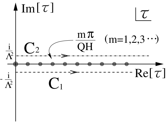
To determine the contribution from the poles on the real $\tau$ axis, we rewrite Eq. (15) in the form

$$V_{\rm eff}(\sigma)=\frac{\sigma^{2}}{4G}+I(\sigma)-I(\sigma=0)+I^{*}(\sigma)-I^{*}(\sigma=0),$$ (16)

where

$$I(\sigma) = \frac{e^{-3\pi i/4}}{(4\pi)^{3/2}\beta}\sum_{n=0}^{\infty}\int_{C_{1}}\!d\tau\frac{QH}{\tau^{3/2}}\cot{(QH\tau)}e^{-i\tau(\omega_{n}-i\mu)^{2}-i\tau\sigma^{2}}.$$ (17)

After the Wick rotation in the complex $\tau$-plane, the contribution from the poles is classified into the following two cases.
a) $\omega_{0}{}^{2}+\sigma^{2}-\mu^{2}=(\pi T)^{2}+\sigma^{2}-\mu^{2}>0$

In this case, the integrand in Eq. (17) converges as $\tau\to-i\infty$. Hence, the expression (17) can be continued to imaginary $\tau$ without encountering any poles:

$$I(\sigma)+I^{*}(\sigma) = \frac{1}{4\pi^{3/2}\beta}\sum_{n=0}^{\infty}\int_{1/\Lambda^{2}}^{\infty}d\tau\ f(\sigma;n;\tau)\ ,$$ (18)

$$f(\sigma;n;\tau) = \frac{QH}{\tau^{3/2}}\coth(QH\tau)\cos(2\omega_{n}\mu\tau)e^{-\tau(\omega_{n}{}^{2}-\mu^{2}+\sigma^{2})}\ .$$ (19)

We can rewrite the summation in this expression by using the elliptic theta function, and doing so, we reproduce the results obtained in Ref. Kane.
b) $\omega_{0}{}^{2}+\sigma^{2}-\mu^{2}=(\pi T)^{2}+\sigma^{2}-\mu^{2}<0$

In this case, the integrand in (17) is exponentially suppressed in the limit $\tau\to-i\infty$ for $n>[N]$ and in the limit $\tau\to+i\infty$ for $n<[N]$, where $N(\sigma)=(\beta\sqrt{\mu^{2}-\sigma^{2}}/\pi-1)/2$ and $[N]$ is the maximum integer smaller than $N$. Thus, we must add the residues of the poles for $n<[N]$. This yields

$$I(\sigma)+I^{*}(\sigma) = \frac{1}{4\pi^{3/2}\beta}\left[\sum_{n>[N]}^{\infty}\int_{1/\Lambda^{2}}^{\infty}d\tau f(\sigma;n;\tau)\right.$$ (20)

$$\quad+\left.\sum_{n=0}^{[N]}\left\{h_{0}(\sigma;n)+h_{j}(\sigma;n)+\int_{1/\Lambda^{2}}^{\infty}d\tau\ g(\sigma;n;\tau)\right\}\right],$$

$$g(\sigma;n;\tau) = \frac{QH}{\tau^{3/2}}\coth(QH\tau)\sin(2\omega_{n}\mu\tau)e^{\tau(\omega_{n}{}^{2}-\mu^{2}+\sigma^{2})}\ ,$$ (21)

$$h_{0}(\sigma;n) = \frac{e^{-i\pi/4}}{2}QH\Lambda\int_{-\pi/2}^{\pi/2}d\theta\ e^{-i\theta/2}\cot(QHe^{i\theta}\Lambda^{2})$$ (22)

$$\hskip 28.45274pt\times\exp[-i\{(\omega_{n}-i\mu)^{2}+\sigma^{2}\}e^{i\theta/\Lambda^{2}}]+(c.c.)\ ,$$

$$h_{j}(\sigma;n) = \frac{2}{\sqrt{\pi}}\sum_{l=1}^{\infty}\left(\frac{QH}{l}\right)^{3/2}e^{-2\pi l\omega_{n}\mu/(QH)}$$ (23)

$$\hskip 28.45274pt\times\sin\left\{\frac{\pi l}{QH}(\omega_{n}{}^{2}-\mu^{2}+\sigma^{2})+\frac{3\pi}{4}\right\}\ .$$

By choosing the contour of the proper time integration carefully, we find explicit expressions for the effective potential with Eqs. (16)-(21), without any ambiguities, even for $\mu\gtrsim T>0$. This result is consistent with the previous results in the simultaneous limits $H\rightarrow 0$ and $1/\Lambda^{2}\rightarrow 0$. For example, the effective potential (16) exactly reproduces the result given in Ref. Ina2 at finite $T$ and $\mu$.

3 Phase structure

In this section, we plot the phase structure of the NJL model at finite $T$, $\mu$ and $H$. For this purpose, we numerically calculated the effective potential (16). The parameters of our model are the coupling constant $G$ and the proper time cutoff $\Lambda$. We fix these parameters to the physical mass scale that reproduces the observed values. Here, it is assumed that the $T$, $\mu$ and $H$ dependences of $G$ and $\Lambda$ are not so strong. Below, we use the values $G=38.7{\rm GeV^{-2}}$ and $\Lambda=0.864{\rm GeV}$ obtained in the appendix.

(a) At $T=0.05~{}{\rm GeV}$, $H=0.18~{}{\rm GeV^{2}}$.	(b) At $T=0.05~{}{\rm GeV}$, $H=0.3~{}{\rm GeV^{2}}$.

(c) At $T=0.01~{}{\rm GeV}$, $H=0.18~{}{\rm GeV^{2}}$.

Figure 2: Behavior of the effective potential with $T$, $\mu$ and $H$ fixed.

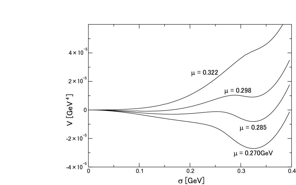
Typical behavior of the effective potential is plotted in Fig. 2. As seen in the figures, we observe the followings:
(a) There is a second order phase transition as $\mu$ is increased, with $T$ kept large and $H$ kept small.
(b) There is a first order phase transition as $\mu$ is increased, with $H$ kept large and fixed.
(c) There are two steps of the transition as $\mu$ is increased, with $T$ and $H$ kept small. First, a first order transition takes place from the third non-vanishing extremum to the first extremum. Next, a second order phase transition occurs where the first non-vanishing extremum disappears.

Figure 3: Dynamical fermion mass $\langle\sigma\rangle$ as a function of the chemical potential $\mu$ at $T=0.01~{}{\rm GeV}$ with $H$ fixed at the typical values $0.0$, $0.10$, $0.18$, $0.21$ and $0.60~{}{\rm GeV^{2}}$.

The ground state is determined by finding the minimum of the effective potential. The necessary condition for this minimum is given by the gap equation

$$\left.\frac{\partial V}{\partial\sigma}\right|_{\sigma=\langle\sigma\rangle}=0,$$ (24)

where $\langle\sigma\rangle$ is the expectation value of $\sigma$, which corresponds to the dynamically generated fermion mass. If the gap equation (24) has more than one solution, we numerically calculate the effective potential for each of these solutions and thereby find the value $\langle\sigma\rangle$ in the ground state. In Fig. 3, we plot the behavior of the dynamical fermion mass $\langle\sigma\rangle$. We find that $\langle\sigma\rangle$ disappears above a certain critical chemical potential. We clearly observe that $\langle\sigma\rangle$ increases continuously as $H$ increases for a small chemical potential. The magnetic field enhances the chiral symmetry breaking. This phenomenon is known as $magnetic~{}catalysis$[7, 8]. For large $\mu$, the behavior of the dynamical fermion mass is different from that in the case of magnetic catalysis. Near the critical chemical potential, a variety of phenomena are observed. For $H=0.10~{}{\rm GeV^{2}}$, there is an oscillation of the critical line. This is called the de Haas-van Alphen effect[12, 23]. It is caused when the Landau levels pass the quark Fermi surface. If $H$ is large enough, the critical chemical potential increases as $H$ increases, and a mass gap exists at the critical value of $\mu$. However, there is a complex behavior of the critical chemical potential for sufficiently small $H$. We observe the two steps of the transition at $H=0.18~{}{\rm GeV}^{2}$.

To understand the situations more precisely, we numerically calculated the critical values of $T$, $\mu$ and $H$ at which the dynamically generated fermion mass disappears. For the second order phase transition, the critical point is obtained by taking the following limit of the gap equation:

$$\lim_{\langle\sigma\rangle\to 0}\left\{~{}\left.\frac{\partial V}{\partial\sigma}\right|_{\sigma=\langle\sigma\rangle}\right\}=0.$$

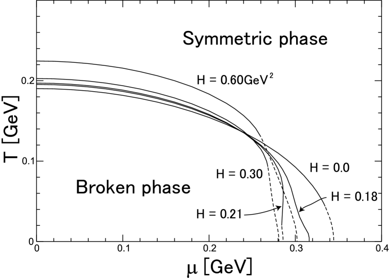
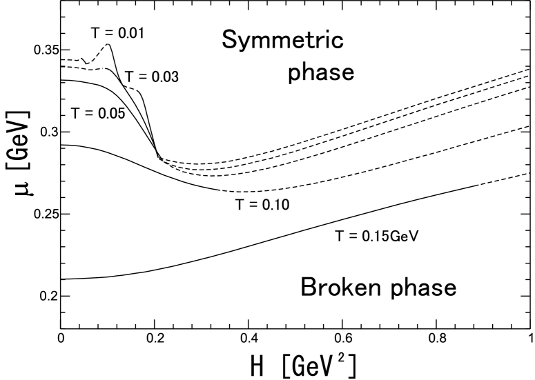
For the first order phase transition, we directly observe the behavior of the effective potential and find the critical point. We plot the phase boundaries in Fig. 4. On the $T$-$\mu$ plane, it is clearly observed that the broken phase spreads out as $H$ is increased for a small chemical potential. The first order phase transition disappears near $H=0.18~{}{\rm GeV^{2}}$.

(a) The $T$-$\mu$ plot with $H$ fixed.	(b) The $H$-$T$ plot with $\mu$ fixed.

(c) The $\mu$-$H$ plot with $T$ fixed.

Figure 4: Critical lines in the $T$-$\mu$ plane, $H$-$T$ plane and $\mu$-$H$ plane. The dashed curve represents the first order phase transition, while the solid curve represents the second order phase transition.

We illustrate the details of the phase boundaries at large chemical potential in the $H$-$T$ and $\mu$-$H$ planes. It is seen that the first and second order phase transitions coexist in the planes. As is seen in Fig. 4(b), the broken phase is separated into two parts for $\mu>0.28~{}{\rm GeV}$. The distortion of the critical line at $\mu=0.34~{}{\rm GeV}$ is caused by the de Haas-van Alphen effect. Such an effect is observed as an oscillating mode for $T\lesssim 0.03~{}{\rm GeV}$ in the $\mu$-$H$ plane in Fig. 4(c). In the parameter range corresponding to the second order phase transition, chiral symmetry breaking is suppressed as $H$ increases, while it is enhanced in the range corresponding to the first order phase transition.

4 Summary

We investigated the phase structure of the NJL model at finite temperature and chemical potential in an external magnetic field. The Fock-Schwinger proper time method was applied to a thermal field theory. Using the two-point function obtained in Ref. IKM, we calculated an effective potential that exactly includes the effects of temperature, chemical potential and constant magnetic field to leading order in the $1/N_{c}$ expansion. We determined the physical contour of the proper time integral. There is no ambiguity with regard to the contour of the proper time integration for $\mu\gtrsim T>0$ in the expression of the effective potential.

We used the current algebra relationship with the current quark mass to determine the mass scale of the model. The position of the tricritical point depends strongly on the mass scale and the regularization procedure. Here, we used the parameter values $G=38.7~{}{\rm GeV^{-2}}$ and $\Lambda=0.864~{}{\rm GeV}$, where the tricritical point appears in the $T$-$\mu$ plane.

Through the study of the shape of the effective potential, we observed a phase transition from the broken phase to the symmetric phase when the temperature $T$, chemical potential $\mu$ and magnetic field $H$ vary. Increasing the temperature and chemical potential tends to prevent the chiral symmetry breaking at $H=0$, while increasing the magnetic field enhances the symmetry breaking at $T=\mu=0$. Therefore, complex behavior of the phase boundary is found with the combined effects of $T$, $\mu$ and $H$, as shown in Fig. 3. We found a two-step transition from the broken phase to the symmetric phase for a medium size magnetic field, $H\sim 0.18~{}$GeV². We found a separation of the broken phase into two parts in the $H$-$T$ plane. With this separation, two tricritical points appear in the critical line for $\mu\sim~{}0.27$ GeV. More than two tricritical points were observed in the critical line for $T\sim 0.01$ GeV in the $\mu$-$H$ plane. In the phase diagram, we observed a contribution from the magnetic field, which is known as magnetic catalysis, and the de Haas-van Alphen effect.

In the present paper, we regard a simple four-fermion interaction model as a low energy effective theory that may possess some fundamental properties of the chiral symmetry breaking in QCD. Although the present work is restricted to an analysis of the phase structure of the four-fermion interaction model with massless quarks, we hope to apply our result to critical phenomena in the real world. In QCD, the current quark mass for up and down quarks is much smaller than the constituent quark mass $\sigma$ for $T=\mu=H=0$. Because the expectation value of $\sigma$ decreases near the critical point, it is no longer valid to ignore the current quark mass. If the contribution from the current quark mass is included in the effective potential, the sharp transitions illustrated in Fig. 4 disappear, as shown in Refs.Suga and Hats:74. In that case, the second order phase transition becomes a cross over.

The strength of the magnetic field that can affect the phase structure is larger than that existing in the core of neuron stars and magnetars. However, an oscillating mode has been observed even for small magnetic fields, and this may have some interesting contribution to the behavior of such stars. Furthermore, we believe that the magnetic field may have been significantly stronger in the early stages of our universe with the primordial magnetic field and that this may have contributed to the critical phenomena in the early universe. To investigate the phenomena exhibited by dense stars, we cannot avoid considering the vortex configurations that generate non-local ground state in the super-fluidity phase. It is necessary to calculate the effective action at finite $\mu$ and $H$. We will continue our work further and extend our analysis to non-local ground states.

Appendix A Physical Scale of $G$ and $\Lambda$

Here we discuss the physical scale of the parameters $G$ and $\Lambda$ of our model. We regard the NJL model as a low energy effective theory of QCD. The parameters should be determined so as to reproduce the observed quantities at low energy scale.

First, we calculate the pion decay constant using the proper time method. The two-point function for a pion composite field is given by

$$\Gamma_{\pi}^{(2)}(p) = -\frac{N_{c}}{G}+iN_{c}\int\frac{d^{4}k}{(2\pi)^{4}}\int d^{3}\vec{x}d^{3}\vec{x}^{\prime}\ e^{-i\vec{k}\cdot\vec{x}}e^{-i(\vec{k}+\vec{p})\cdot\vec{x}^{\prime}}$$ (25)

$$\hskip 56.9055pt\times{\rm tr}[(-i\gamma^{5}\tau^{a})S(\vec{x},0;k_{0})(-i\gamma^{5}\tau^{b})S(\vec{x}^{\prime},0;k_{0}+p_{0})],$$

where $S(\vec{x},\vec{y};k_{0})$ is the quark Green function defined by

$$(\gamma^{0}k_{0}+i\gamma^{j}\partial_{j}-\sigma)S(\vec{x},\vec{y};k_{0})=\delta^{3}(\vec{x}-\vec{y}).$$ (26)

Here, $\sigma$ is determined by finding the stationary point of the effective potential which is determined as a function of $G$ and $\Lambda$. Using the proper time method, the Green function $S(\vec{x},\vec{y};k_{0})$ can be written

$$S(\vec{x},\vec{y};k_{0})=\frac{e^{\pi i/4}}{(4\pi)^{3/2}}(i\gamma^{j}\partial_{j}+\gamma^{0}k_{0}+\sigma)\int^{-0}_{-\infty}\!\frac{d\tau}{\tau^{3/2}}\exp{\left\{-\frac{i}{4}\frac{(\vec{x}-\vec{y})^{2}}{\tau}+i(\sigma^{2}-k_{0}^{2})\tau\right\}},$$ (27)

where $\tau$ is the proper time. Substituting Eq. (27) into Eq. (25), and performing the integration over $k$, $x$ and $x^{\prime}$, we obtain

$$\Gamma_{\pi}^{(2)}(p) = -\frac{N_{c}}{G}+\frac{N_{c}}{2\pi^{2}}\int^{\infty}_{+0}d\tau ds\ e^{-i\sigma^{2}(\tau+s)}e^{ip^{2}\tau s/(\tau+s)}$$ (28)

$$\hskip 56.9055pt\times\frac{1}{(\tau+s)^{2}}\left[\frac{1}{\tau+s}\left\{2i-p^{2}\frac{\tau s}{\tau+s}\right\}-\sigma^{2}\right].$$

The renormalization constant for the pion wave function is defined by $\Gamma_{\pi}^{(2)}(p^{2})=Z_{\pi}^{-1}p^{2}+O(p^{4})$. After applying the Wick rotation to Eq. (28) the renormalization constant $Z_{\pi}$ is derived as

$$Z_{\pi}^{-1}=\frac{N_{c}}{2\pi^{2}}\int^{\infty}_{+0}d\tau ds\ e^{-\sigma^{2}(\tau+s)}\frac{\tau s}{(\tau+s)^{3}}\left(\frac{3}{\tau+s}+\sigma^{2}\right)\ .$$ (29)

To obtain the relationship between $f_{\pi}$ and $Z_{\pi}$, we evaluate the order parameter of the chiral symmetry breaking, $[iQ_{5}^{a},\pi^{b}]$, where $Q_{5}^{a}$ is the conserved axial charge and $\pi^{a}$ is the asymptotic pion field. Then, using the conserved axial current $j_{\mu}^{a}(x)$, we obtain

$$\left<0\left|[iQ_{5}^{a},\pi^{b}]\right|0\right> = \langle 0|[\int\!d^{3}\vec{x}~{}j^{a}_{0}(x),\pi^{b}]|0\rangle$$ (30)

$$= \int\!d^{4}x~{}i\partial^{\mu}\left<0\left|Tj^{a}_{\mu}(x)\pi^{b}\right|0\right>.$$

The pion decay constant $f_{\pi}$ is defined by

$$\left<0\left|j^{a}_{\mu}(x)\right|\pi(p)\right>=-if_{\pi}\delta^{ab}p_{\mu}e^{-ipx}.$$ (31)

This implies that

$$j^{a}_{\mu}(x)=f_{\pi}\partial_{\mu}\pi^{a}(x)+\cdots.$$ (32)

Substituting Eq. (32) into Eq. (30), we obtain

$$\left<0\left|[iQ^{a}_{5},\pi^{b}]\right|0\right>=f_{\pi}\delta^{ab}.$$ (33)

On the other hand, $j^{a}_{\mu}(x)$ and $\pi^{a}(x)$ are described by the quark field $\psi(x)$ as

$$j^{a}_{\mu}(x)=\bar{\psi}\gamma_{\mu}\gamma_{5}\frac{\tau^{a}}{2}\psi\quad,\quad\pi^{a}(x)=-\frac{G}{N_{c}}Z_{\pi}^{-1/2}\bar{\psi}i\gamma_{5}\tau^{a}\psi.$$ (34)

Inserting Eq. (34) into the second line of Eq. (30), we find

$$\left<0\left|[iQ^{a}_{5},\pi^{b}]\right|0\right>=-\frac{G}{N_{c}}Z_{\pi}^{-1/2}\left<0\left|-\bar{\psi}\psi\right|0\right>\delta^{ab}=-Z_{\pi}^{-1/2}\sigma\delta^{ab}.$$ (35)

Comparing (33) with (35), we obtain the relationship $f_{\pi}=-Z_{\pi}^{-1/2}\sigma$. From Eq. (29) and this relationship, it is found that the pion decay constant can be expressed as a function of $\sigma$ and $\Lambda$,

$$f_{\pi}{}^{2}=\frac{N_{c}\sigma^{2}}{2\pi^{2}}\int_{1/\Lambda^{2}}^{\infty}d\tau\frac{1}{2\tau}\left\{e^{-\sigma^{2}\tau}(1-\sigma^{2}\tau)-\sigma^{4}\tau^{2}{\rm Ei}(-\sigma^{2}\tau)\right\},$$ (36)

where ${\rm Ei}(-x)$ is the exponential-integral function.

We determine the relationship between $G$ and $\Lambda$ such that the measured value, $f_{\pi}=93~{}{\rm MeV}$, is reproduced, as shown in Fig. 5.

Figure 5: Relationship between $G$ and $\Lambda$.

The phase structure in the $T$-$\mu$ plane differs dramatically for values of $G$ and $\Lambda$ on the solid curve (case i) and the dashed curve (case ii) in Fig. 5. Evaluating the effective potential, we plot the typical behavior of the critical line in $T$-$\mu$ plane in both cases. As shown in Fig. 6, only the second order phase transition takes place in case i, while the first and second order phase transitions coexist in case ii, and a tricritical point appears on the critical line. These results agree with the well-known result obtained using the other regularization procedure.[2, 5, 21] Therefore, we choose the mass scale in a range corresponding to case ${\bf ii}$. In chiral limit, we determine only the curve in the $G$-$\Lambda$ plane.

Figure 6: Critical lines at $H=0$ in the cases i and ii. The dashed curve represents the first order phase transition, while the solid curve represents the second order phase transition.

To determine the values of $G$ and $\Lambda$ in this range, we evaluate the pion mass. As is well known, the pion is a massless Goldstone mode if the explicit chiral symmetry breaking is not accounted for. In QCD, a small quark mass breaks the chiral symmetry. The pion decay constant is proportional to $\sigma$. Because the value of $\sigma$ is much larger than the current quark mass, we ignore the a contribution from the current quark mass when calculating the pion decay constant. However, to evaluate the realistic pion mass, $m_{\pi}=138~{}{\rm MeV}$, we consider the influence of the current quark mass.

Accounting for the current quark mass, the axial current is not conserved, and we have

$$\partial^{\mu}j^{a}_{\mu}(x)=\hat{m}\bar{\psi}i\gamma_{5}\tau^{a}\psi(x),$$ (37)

where $\hat{m}$ is the current quark mass, $2\hat{m}=m_{u}+m_{d}$. Substituting Eq. (31) into Eq. (37), we obtain

$$\widehat{m}\left<0\left|\bar{\psi}i\gamma_{5}\tau^{a}\psi(0)\right|\pi^{b}(p=0)\right>=-f_{\pi}m_{\pi}^{2}\delta^{ab}.$$ (38)

Similarly to Eqs. (30) and (33), we obtain

$$-f_{\pi}\left<0\left|\bar{\psi}i\gamma_{5}\tau^{a}\psi(0)\right|\pi^{b}(p=0)\right>=\left<0\left|\bar{\psi}\psi\right|0\right>$$ (39)

in the chiral limit. Therefore, the pion mass is obtained as

$$(f_{\pi}m_{\pi})^{2}=-\frac{N_{c}}{G}~{}\hat{m}\langle\sigma\rangle,$$ (40)

to first order in the current quark mass.[20] This is known as the Gell-Mann$-$Oakes$-$Renner relation.

From the measured values $f_{\pi}=93~{}{\rm MeV}$ and $m_{\pi}=138~{}{\rm MeV}$ and Eqs. (36) and (40), we obtain the matching condition for the coupling constant $G$ and the proper time cutoff $\Lambda$ with the physical scale. These parameters are extracted as functions of $\hat{m}$. For $\hat{m}=5.5~{}{\rm MeV}$, the parameters $G$ and $\Lambda$ are found to be

$$G=25.4~{}{\rm GeV^{-2}}\quad,\quad\Lambda=0.991~{}{\rm GeV},$$ (41)

which are located in the range of the solid curve in Fig. 5. A larger current quark mass is realized on the dashed curve in Fig. 5. If we set $\hat{m}=7.0~{}{\rm MeV}$ in Eq. (40), the parameters $G$ and $\Lambda$ are fixed as

$$G=38.7~{}{\rm GeV^{-2}}\quad,\quad\Lambda=0.864~{}{\rm GeV},$$ (42)

which are in the range of the dashed curve in Fig. 5.

It should be noted that we consider the contribution from the current quark mass only for the purpose of determining the values of $G$ and $\Lambda$.