Dynamics of MSSM flat directions consisting of multiple scalar fields

Abstract

Although often chosen because of simplicity, a single scalar field does not provide a general parametrization of an MSSM flat direction. We derive a formalism for a class of gauge invariant polynomials which result in a multifield description of the flat directions. In contrast to the single field case, the vanishing of the gauge currents yields an important dynamical constraint in the multifield framework. We consider in detail the example of the $H_{u}L$ flat direction and study the dynamical evolution during and after inflation. We highlight the differences between the single and the multifield flat directions. We show that in the multifield case the field space has an intrinsic curvature and hence unsuppressed non-minimal kinetic terms for the flat direction scalars arise. Also the phases of the individual components evolve non-trivially right after inflation, charging the components of the condensate and producing an enhanced entropy after the decay of the condensate, which is due to cross-coupling of different lepton flavours in the F term. However, the qualitative features of the single field Affleck-Dine baryogenesis, such as the produced total charge, remain largely unchanged.

HIP-2003-59/TH

kari.enqvist@helsinki.fi, asko.jokinen@helsinki.fi, anupamm@hep.physics.mcgill.ca

1 Introduction

Supersymmetric gauge theories come with gauge invariant polynomials along which the scalar potential vanishes at a classical level [2]. These correspond to the flat directions in the moduli space of the scalar fields. Within the Minimal Supersymmetric Standard Model (MSSM) the classical potential is given by the sum of the $F$ and $D$ term contributions, which vanish individually along these flat directions. Flatness is however lifted by soft supersymmetry breaking, but a non-renormalization theorem guarantees that the flat direction does not obtain any renormalizable perturbative superpotential correction [3]. However, non-perturbative (supergravity-induced) corrections will also lift the flatness.

MSSM flat directions can give rise to a host of cosmologically interesting dynamics (for a review, see [4]). These include Affleck-Dine baryogenesis [5, 6, 7], the cosmological formation and fragmentation of the MSSM flat direction condensate and subsequent $Q$-ball formation [8, 9, 10, 11], reheating the Universe with $Q$-ball evaporation [12], generation of baryon isocurvature density perturbations [13], as well as curvaton scenarios where MSSM flat directions reheat the Universe and generate adiabatic density perturbations [14]. Adiabatic density perturbations induced by fluctuating inflaton-MSSM flat direction coupling has also been discussed [15].

In the MSSM all the flat directions have been parameterized by gauge invariant monomials [7, 16]. In such a case the MSSM flat direction is some linear combination of the MSSM scalars and can be thought of as a trajectory in the moduli space described by a single scalar degree of freedom. A simple example is the $H_{u}L$ flat direction $\phi$, defined as $(H_{u})_{1}=L_{2}=\phi/\sqrt{2}$ (indices here label SU(2)). However, a flat direction can also be constructed as a gauge invariant polynomial, where the previously mentioned monomials generate the polynomial. This means that the flat direction is a non-linear combination of the MSSM fields. It no longer can be described by a single scalar field. Such a gauge invariant polynomial, rather than a monomial, is needed e.g. when for $H_{u}L$ instead of a single leptonic generation one considers simultaneously all three.

The purpose of the present paper is to illustrate the dynamics of Affleck-Dine condensate described by a gauge invariant polynomial. Previously Senami and Yamamoto [17] have considered such a case in MSSM and its extensions but they used an extrinsic point of view without gauge invariant polynomials. We will discuss the dynamics from an intrinsic point of view i.e. using coordinates that describe only the behaviour of the flat direction. Given that the flat direction is the minimum of energy the two approaches are equivalent.

We will also discuss how a non-renormalizable superpotential correction can lift such a multi-field flat direction. We will highlight the formation and charge conservation of the condensate along with the gauge conditions required to be satisfied. In the present paper we will mostly restrict ourselves to a simple example of a flat direction involving $L$ and $H_{u}$ (”the $H_{u}L$ flat direction”), which is a linear combination of superfields, and study its dynamical evolution through the cosmic history of the Universe.

We begin our discussion with the basic definitions of the flat directions in $N=1$ supersymmetry in Section 2. In Section 3 we first construct $H_{u}L$ flat direction parameterized by a gauge invariant monomial. We then discuss gauge invariant polynomials which are $F$ and $D$ flat at the level of unbroken supersymmetry and write down the equation of motion for the $H_{u}L$ scalars with the help of two projection operators, defined in the Appendix. Vanishing of the gauge currents is carefully accounted for. to In Section 4 we write down the multifield scalar potential, accounting for supersymmetry breaking and non-renormalizable superpotential corrections. In Section 5 we discuss qualitatively the dynamical behavior of the $H_{u}L$ condensate consisting, comparing it with single field case. Section 6 presents the results numerical studies for the multifield trajectories, charge densities and charge asymmetries. In Section 7 we make concluding remarks and discuss the physical implications of the results.

2 General features of flat directions

The scalar potential of supersymmetric theories is given by [18]

$$\mbox{$$}V=\frac{1}{2}\sum_{A}D^{A}D^{A}+\sum_{i}\left|{{\partial W}\over{\partial\phi_{i}}}\right|^{2}\,,\vspace{\undereqskip}$$ (1)

where $W$ is the superpotential and the D-flat directions are solutions to

$$\mbox{$$}D^{A}=\sum_{i}\phi_{i}^{\dagger}T^{A}\phi_{i}=0\,,\vspace{\undereqskip}$$ (2)

where $\phi_{i}$ are the scalar fields and $T^{A}$ are the generators of the symmetry group, which for $SU(n)$can be chosen to be Hermitian and traceless. Making a gauge transformation

$$\mbox{$$}\phi_{i}\to U(x)\phi_{i}\,\vspace{\undereqskip}$$ (3)

transforms the D-term in Eq. (2) to

$$\mbox{$$}D^{A}\to\sum_{i}\phi_{i}^{\dagger}U(x)^{-1}T^{A}U(x)\phi_{i}=\sum_{i}\phi_{i}^{\dagger}\tilde{T}^{A}\phi_{i}\,,\vspace{\undereqskip}$$ (4)

where $\tilde{T}^{A}$ is also hermitian and traceless. Since $T^{A}$ are basis for traceless hermitian matrices, then $\tilde{T}^{A}$ can be written as $\tilde{T}^{A}=c^{AB}T^{B}$ with $c^{AB}$ as complex coefficients. Hence the D-term, Eq. (4) reads

$$\mbox{$$}D^{A}\to c^{AB}D^{B}=0\,,\vspace{\undereqskip}$$ (5)

where Eq. (2) was used in the last step, proving that Eq. (2) is gauge invariant. The solutions, Eq. (5), are gauge orbits. (This can be generalized to other gauge groups by virtue of Baker-Campbell-Hausdorff formula or in general quoting that D term transforms as a vector in the adjoint representation, which essentially have been shown to be the case for $SU(N)$).

One should also specify the gauge field configuration related to the scalar field because it is changed by a gauge transformation. The minimum energy is obtained with pure gauge configurations $F_{\mu\nu}^{A}=0$. The equation of motion for the gauge field is

$$\mbox{$$}D^{\nu}F_{\mu\nu}^{A}=J_{\mu}^{A}\,,\vspace{\undereqskip}$$ (6)

where $J_{\mu}^{A}$ is the matter current defined by

$$\mbox{$$}J_{\mu}^{A}=i\sum_{i}\left((D_{\mu}\phi_{i})^{\dagger}T^{A}\phi_{i}-\phi_{i}^{\dagger}T^{A}(D_{\mu}\phi_{i})\right)\,.\vspace{\undereqskip}$$ (7)

With a pure gauge configuration the left hand side of Eq. (6) vanishes, providing a constraint on the matter current Eq. (7), and a relationship between the flat direction and gauge fields. Choosing a gauge corresponds to picking a scalar field value and the gauge field value from the gauge orbit.

Minimizing the energy of the configurations, i.e.the equation of motion, requires that $D_{\mu}\phi_{i}=0$. This of course results into vanishing current in Eq. (7). With the gauge choice, $A_{\mu}^{A}=0$, the scalar fields would then have to be constants. However, once SUSY breaking is included, the scalar fields become dynamical and the condition on the minimum energy becomes more subtle. For a homogeneous scalar field one can check that the minimum of energy is still obtained by a pure gauge configuration, despite the fact that the scalar fields have a non-vanishing energy. Therefore the current Eq. (7) has to vanish, but now $D_{0}\phi_{i}\neq 0$. This is a constraint on the cosmological dynamics of MSSM condensates that has to be satisfied.

Let us remark that for inhomogeneous fields the situation is even more complicated. The minimum of energy still obeys the equation of motion Eq. (6), but it is no longer obvious that the minimum is obtained with a pure gauge configuration and a zero current. In fact, a more likely situation is that a spatially varying condensate, implying a spatially varying gauge charge, will give rise to non-vanishing currents and non-trivial gauge configurations. In the present paper we do not consider inhomogeneous condensates, but if one were to study the spatial fluctuations of the flat direction inhomogeneities would have to be taken into account.

The solutions of Eq. (2) can be parameterized by analytic gauge invariant polynomials $I(\{\phi_{i}\})$ [2, 19] which can be obtained by solving

$$\mbox{$$}{{\partial I}\over{\partial\phi_{i}}}=C\phi_{i}^{*}\,,\vspace{\undereqskip}$$ (8)

where $C$ is a complex coefficient . This equation is also gauge invariant and therefore acts as a solution to a gauge orbit. The geometrical significance of Eq. (8) is that the polynomial $I$ defines level surfaces, e.g. $I(\phi)=B=const.$, which actually are the gauge orbits of the complexified gauge group. Then the flat direction corresponds to the minimum of the norm, $|\phi|=\sqrt{\sum_{i}|\phi_{i}|^{2}}$, which turns out to be orthogonal to $\phi$. For analytic functions the complex conjugate of the gradient is orthogonal to the level surface. This leads to Eq. (8) which just states that the gradient of $I$ and the complex conjugate of $\phi$ have to be parallel (for details see [19]).

If the polynomial describing the flat direction is actually a monomial and is composed of $N$ scalar fields of the model, then from Eq. (8) it follows that there are $N$ complex equations for $N+1$ complex variables, $\phi_{i}$, and $C$. Therefore there is at least one complex degree of freedom left, which can be chosen to be the scalar field parameterizing the flat direction. In case of flat directions parameterized by multiple scalar fields, the relevant polynomial is a sum of monomials $I_{i}$ such that $I=\sum_{i}c_{i}I_{i}$, where $c_{i}$ are complex coefficients . As a consequence, there appear extra complex degrees of freedom.

3 Example: $H_{u}L$ flat directions

3.1 $H_{u}L$ parameterized by single scalar field

A generic treatment of polynomials generating MSSM flat directions is beyond the scope of the present paper. Rather, in order to gain some insight on the dynamics of flat directions with multiple fields, we focus on a simple example, the $H_{u}L$ flat direction. Let us begin by reiterating the case for a single generation of leptons, denoted here as $L$. The relevant monomial is then given by [7, 16]

$$\mbox{$$}I=H_{u}L=\epsilon_{\alpha\beta}H_{u}^{\alpha}L^{\beta}\,.\vspace{\undereqskip}$$ (9)

Applying the constraint Eq. (8), one obtains two equations

$$\mbox{$$}{{\partial I}\over{\partial H_{u}^{\alpha}}} = \epsilon_{\alpha\beta}L^{\beta}=C(H_{u}^{\alpha})^{*}\,,$$

$${{\partial I}\over{\partial L^{\alpha}}} = \epsilon_{\beta\alpha}H_{u}^{\beta}=C(L^{\alpha})^{*}\,.\vspace{\undereqskip}$$ (10)

By taking the absolute values of the equations, it follows that $|C|=1$ and $|H_{u}^{1}|=|L^{2}|,\,|H_{u}^{2}|=|L^{1}|$. By multiplying the first equation by $L^{\alpha}$ and summing over $\alpha$, one obtains that $H_{u}\perp L$. Hence the general structure of $H_{u}L$ is given by

$$\mbox{$$}H_{u}=\left(\begin{array}[]{ll}\phi\\ \chi\end{array}\right),\qquad L=e^{i\zeta}\left(\begin{array}[]{ll}-\chi^{*}\\ \phi^{*}\end{array}\right)\,,\vspace{\undereqskip}$$ (11)

where $\phi,\,\chi$ are complex scalar fields and $\zeta$ is a real scalar field.

Let us now apply the current constraint $J_{\mu}^{A}=0$ as given by Eq. (7). In the case of single leptonic generation we can write it as

$$\mbox{$$}J_{\mu}^{A}=i\left((D_{\mu}H_{u})^{\dagger}T^{A}H_{u}-H_{u}^{\dagger}T^{A}D_{\mu}H_{u}+(D_{\mu}L)^{\dagger}T^{A}L-L^{\dagger}T^{A}D_{\mu}L\right)=0\,,\vspace{\undereqskip}$$ (12)

where $T^{A}$ are the $SU(2)\times U(1)$-generators so that there are four equations altogether. Since the current is gauge invariant, we can choose a gauge, and since the gauge is pure, we may choose $A_{\mu}^{A}=0$. (The details of the calculation is left to the next subsection, see Eq. (33)). As is well known, the final result turns out to be

$$\mbox{$$}H_{u}=\frac{1}{\sqrt{2}}\left(\begin{array}[]{ll}\phi\\ 0\end{array}\right),\qquad L=\frac{1}{\sqrt{2}}\left(\begin{array}[]{ll}0\\ \phi\end{array}\right)\,,\vspace{\undereqskip}$$ (17)

where $\phi$ is a complex scalar field.

One has to check that Eq. (17) is also F-flat. The F-terms are obtained from the superpotential

$$\mbox{$$}W=\lambda_{u}QH_{u}\bar{u}+\lambda_{d}QH_{d}\bar{d}+\lambda_{e}LH_{d}\bar{e}+\mu_{H}H_{u}H_{d}\,,\vspace{\undereqskip}$$ (18)

where $\lambda_{u},\,\lambda_{d},\,\lambda_{e}$ are the Yukawa couplings, family, colour and $SU(2)$ indices are suppressed. One can easily find that the $H_{u}L$ is automatically F-flat except for the $\mu_{H}$-term in the last equation. However, since $\mu_{H}$ is of the order of the SUSY breaking mass, and, since SUSY breaking terms anyway lift the flat direction, the $\mu_{H}$-terms can be neglected at this stage. The Lagrangian along the $H_{u}L$ direction reads simply as

$$\mbox{$$}{\cal L}=|\partial_{\mu}H_{u}|^{2}+|\partial_{\mu}L|^{2}-V=|\partial_{\mu}\phi|^{2}-V(\phi)\,.\vspace{\undereqskip}$$ (19)

3.2 $H_{u}L$ parametrized by three scalar fields

In principle, the discussion above applies separately for each lepton generation. However, apart from pure chance, there is no physical mechanism that would pick out one generation over the others. Hence a most natural possibility would be to consider $H_{u}L$ parametrized by all three leptonic degrees of freedom. Therefore we should consider the gauge invariant polynomial

$$\mbox{$$}I=\nu_{1}H_{u}L_{1}+\nu_{2}H_{u}L_{2}+\nu_{3}H_{u}L_{3}\,,\vspace{\undereqskip}$$ (20)

where $\nu_{i}$ are complex coefficients (of which one can be freely chosen). The D-flatness equations Eq. (8) become (compare with Eq. (3.1))

$$\mbox{$$}{{\partial I}\over{\partial H_{u}^{\alpha}}} = \sum_{i=1}^{3}\nu_{i}\epsilon_{\alpha\beta}L_{i}^{\beta}=C(H_{u}^{\alpha})^{*}\,,$$

$${{\partial I}\over{\partial L_{i}^{\alpha}}} = \nu_{i}\epsilon_{\beta\alpha}H_{u}^{\beta}=C(L_{i}^{\alpha})^{*}\,.\vspace{\undereqskip}$$ (21)

By solving $L_{i}^{\alpha}$ from the second equation and inserting into the first, one obtains the constraint

$$\mbox{$$}|C|^{2}=\sum_{i=1}^{3}|\nu_{i}|^{2}\,.\vspace{\undereqskip}$$ (22)

Working the other way around, i.e.  by solving $H_{u}^{\alpha}$ from the first equation and inserting into the second, one obtains a matrix equation

$$\mbox{$$}P(\mathbf{L}^{\alpha})^{*}=(\mathbf{L}^{\alpha})^{*},\qquad P_{ij}=\frac{\nu_{i}\nu_{j}^{*}}{\sum_{k}|\nu_{k}|^{2}}\,,\vspace{\undereqskip}$$ (23)

where $\mathbf{L}^{\alpha}=(L_{1}^{\alpha},L_{2}^{\alpha},L_{3}^{\alpha})^{T}$ is a vector in flavor space and $P$ is a projection matrix to the vector $\mathbf{\nu}=(\nu_{1},\nu_{2},\nu_{3})^{T}$. Note that Eq. (23) can be fulfilled only if $(\mathbf{L}^{\alpha})^{*}$ is parallel to $\mathbf{\nu}$ so that

$$\mbox{$$}(\mathbf{L}^{\alpha})^{*}=c^{\alpha}\mathbf{\nu}\,,\vspace{\undereqskip}$$ (24)

where $c^{\alpha}$ is a complex coefficient. The flat direction is given by

$$\mbox{$$}L_{i}=\nu_{i}^{*}\left(\begin{array}[]{ll}c^{1*}\\ c^{2*}\end{array}\right),\quad H_{u}=e^{i\delta_{C}}\sqrt{\sum_{i}|\nu_{i}|^{2}}\left(\begin{array}[]{ll}c^{2}\\ -c^{1}\end{array}\right)\,,\vspace{\undereqskip}$$ (25)

where $\delta_{C}$ is the phase of $C$ which was left undetermined in Eq. (22). Making redefinitions $\phi_{i}=\nu_{i}^{*}c^{2*}$, $\psi=c^{1*}/c^{2*}$ and $\delta_{C}=\chi-\delta_{2}$, where $\chi$ is real field and $\delta_{2}$ is the phase of $c^{2}$, one obtains a simplified expression for the field content of the $H_{u}L$-flat direction

$$\mbox{$$}L_{i}=\phi_{i}\left(\begin{array}[]{ll}\psi\\ 1\end{array}\right),\quad H_{u}=e^{i\chi}\sqrt{\sum_{i}|\phi_{i}|^{2}}\left(\begin{array}[]{ll}1\\ -\psi^{*}\end{array}\right)\,.\vspace{\undereqskip}$$ (26)

Let us now apply the current constraint $J_{\mu}^{A}=0$ Eq. (7), where

$$\mbox{$$}J_{\mu}^{A}=i((D_{\mu}H_{u})^{\dagger}T^{A}H_{u}-H_{u}^{\dagger}T^{A}D_{\mu}H_{u})+i\sum_{i}((D_{\mu}L_{i})^{\dagger}T^{A}L_{i}-L_{i}^{\dagger}T^{A}D_{\mu}L_{i})\,.\vspace{\undereqskip}$$ (27)

We find

$$\mbox{$$}J_{\mu}^{Y} = \frac{i}{2}\left[(1+|\psi|^{2})\left(\sum_{i}J_{i}^{\phi}-2i\sum_{k}|\phi_{k}|^{2}\partial_{\mu}\chi\right)+2\sum_{k}|\phi_{k}|^{2}J^{\psi}\right]=0\,,$$ (28)

$$J_{\mu}^{3} = \frac{i}{2}\left[(1-|\psi|^{2})\left(\sum_{i}J_{i}^{\phi}-2i\sum_{k}|\phi_{k}|^{2}\partial_{\mu}\chi\right)-2\sum_{k}|\phi_{k}|^{2}J^{\psi}\right]=0\,,$$ (29)

$$J_{\mu}^{1+i2} = i\left[-\psi^{*}\left(\sum_{i}J_{i}^{\phi}-2i\sum_{k}|\phi_{k}|^{2}\partial_{\mu}\chi\right)+2\sum_{k}|\phi_{k}|^{2}\partial_{\mu}\psi^{*}\right]=0\,,\vspace{\undereqskip}$$ (30)

where

$$\mbox{$$}J_{i}^{\phi}\equiv\phi_{i}^{*}\partial_{\mu}\phi_{i}-\phi_{i}\partial_{\mu}\phi_{i}^{*},~{}~{}J^{\psi}\equiv\psi^{*}\partial_{\mu}\psi-\psi\partial_{\mu}\psi^{*}\,.\vspace{\undereqskip}$$ (31)

Adding Eqs. (28, 29) together, we obtain

$$\mbox{$$}\partial_{\mu}\chi=\frac{\sum_{j}J_{j}^{\phi}}{2i\sum_{k}|\phi_{k}|^{2}}\,.\vspace{\undereqskip}$$ (32)

Using Eqs. (32, 30), one obtains $\partial_{\mu}\psi=0$, so that $\psi=const.$ Therefore we may gauge it away by a global $U(1)$ transformation including it in the normalization of $\phi_{i}$. Hence we finally obtain

$$\mbox{$$}L_{i}=\phi_{i}\left(\begin{array}[]{ll}0\\ 1\end{array}\right),\quad H_{u}=e^{i\chi}\sqrt{\sum_{i}|\phi_{i}|^{2}}\left(\begin{array}[]{ll}1\\ 0\end{array}\right)\,,\vspace{\undereqskip}$$ (33)

where $\chi$ is given in Eq. (32). Since the final configuration is three complex dimensional which is the maximal dimension of the flat direction [16] containing $H_{u}$ and $L_{i}$, the polynomial Eq. (20) gives a complete characterization of the $H_{u}L$ flat direction.

3.3 The effective Lagrangian for the multiple flat direction

For one scalar field the constraint for the phase $\chi$ in Eq. (32) reduces to $\partial_{\mu}\chi=\partial_{\mu}\theta$, where $\theta$ is the phase of the scalar field $\phi=|\phi|\exp(i\theta)$. Therefore, up to a normalization, the field configuration reduces to Eq. (17). However, for more than one scalar field, the constraint Eq. (32) is not necessarily solvable. The problem is the following: on the right hand side there is a vector field (formed as a sum of the scalar fields $\phi_{i}$ and their derivatives), on the left hand side there is a gradient of the scalar function, so the right hand side has to be rotationless (in the language of differential forms the one-form on the right-hand side has to be closed for it to be exact). The necessary (and in simply connected space sufficient) condition for the vector field to be a gradient of a scalar function is

$$\mbox{$$}(\partial_{\mu}\partial_{\nu}-\partial_{\nu}\partial_{\mu})\chi=0\,,\vspace{\undereqskip}$$ (34)

which yields

$$\mbox{$$}\partial_{\mu}\Phi^{\dagger}\,(1-P_{1}-P_{2})\,\partial_{\nu}\Psi=0\,,\vspace{\undereqskip}$$ (35)

where the $P_{i}$ are projection operators discussed in the Appendix.

From Eq. (35) one sees that the components of the gradient are constrained to be orthogonal outside of the two-dimensional surface spanned by $\Phi$ and $\Psi$. On the surface there are no constraints. If there is only one scalar field, then $\Phi$ and $\Psi$ are two-dimensional and Eq. (35) is trivially satisfied, since in this case $P_{1}+P_{2}=1$. If the scalar fields do not depend on space or time, then the constraint is trivially satisfied. If the fields depend only on one coordinate (time or one of the spatial coordinates; homogeneous fields fall into this category), then again one can show that the constraint is trivially satisfied. Since in the cosmological context the large scale homogeneity is a reasonable approximation, we do not have to worry here about not fulfilling Eq. (35).

The dynamical evolution of the multiple field flat direction is determined by the MSSM Lagrangian

$$\mbox{$$}\mathcal{L}=|\partial_{\mu}H_{u}|^{2}+\sum_{i=1}^{3}|\partial_{\mu}L_{i}|^{2}-V\,,\vspace{\undereqskip}$$ (36)

It turns out to be convenient to change the parameterization of the flat direction by a phase shift to

$$\mbox{$$}L_{i}=e^{-i\chi/2}\phi_{i}\left(\begin{array}[]{ll}0\\ 1\end{array}\right),\quad H_{u}=e^{i\chi/2}\sqrt{\sum_{i}|\phi_{i}|^{2}}\left(\begin{array}[]{ll}1\\ 0\end{array}\right)\,,\vspace{\undereqskip}$$ (37)

where $\chi$ is solved from Eq. (32). Now the Lagrangian is obtained by inserting Eq. (37) into Eq. (36)

$$\mbox{$$}\mathcal{L}=\frac{1}{2}\partial_{\mu}\Phi^{\dagger}\left(1+P_{1}-\frac{1}{2}P_{2}\right)\partial^{\mu}\Phi-V\,,\vspace{\undereqskip}$$ (38)

(for the projection operators $P_{i}$, see Appendix). Note that there are now non-minimal kinetic terms. This is due to the fact that the $H_{u}L$ direction is a curved sub-manifold of the whole field manifold, as can be seen from Eq. (37) which implies that, up to a gauge choice, the sub-manifold is actually a sphere. In the one-field case the flat direction is formed only along a one-dimensional sub-manifold and therefore has vanishing curvature. The equations of motion resulting from Eq. (38) are (see Appendix for details)

$$\mbox{$$}\partial_{\mu}\partial^{\mu}\Phi+3H\dot{\Phi}+\left(1-\frac{1}{2}P_{1}+P_{2}\right){{\partial V}\over{\partial\Phi^{\dagger}}}-N^{-1}\left[\partial_{\mu}\Psi\,(\Psi^{\dagger}\partial^{\mu}\Phi)\right.$$

$$\hbox to0.0pt{\hss${}+{}$}\left.\Psi\,(\partial_{\mu}\Psi^{\dagger}P_{2}\partial^{\mu}\Phi)+\frac{1}{2}\Phi\,\partial_{\mu}\Phi^{\dagger}\left(1-P_{1}-\frac{3}{2}P_{2}\right)\partial^{\mu}\Phi\right]=0,\vspace{\undereqskip}$$ (39)

where $N=\Phi^{\dagger}\Phi$.

Since we are interested in the background dynamics, the partial derivatives can be replaced by time derivatives. In that case the different terms have analogues in classical mechanics. On the first row the potential gradient is deformed by two projections: $P_{1}$ makes the potential flatter and $P_{2}$ steeper in the directions $\Phi$ and $\Psi$ respectively. The last term on the second row generalizes centripetal acceleration. The rest two terms are analogous to the Coriolis and Euler forces.

4 The potential for $H_{u}L$

In the real world supersymmetry is broken. This lifts the degeneracy of the vacuum solutions of the supersymmetric gauge theory, and the flat directions become dynamical fields [6, 7]. Here we just list the contributions relevant for $H_{u}L$.

The soft SUSY breaking mass parameters together with the $\mu$-term read

$$\mbox{$$}(m_{H_{u}}^{2}+\mu_{H}^{2})|H_{u}|^{2}+\sum_{i}m_{L_{i}}^{2}|L_{i}|^{2}=\sum_{i}m_{\phi_{i}}^{2}|\phi_{i}|^{2}\,,\vspace{\undereqskip}$$ (40)

where

$$\mbox{$$}m_{\phi_{i}}^{2}=m_{H_{u}}^{2}+\mu_{H}^{2}+m_{L_{i}}^{2}\,.\vspace{\undereqskip}$$ (41)

The mass parameters $m_{\phi_{i}}$ are of the order of the soft SUSY breaking mass $m_{S}$, which in the gravity mediated SUSY breaking scenario is the gravitino mass $m_{3/2}$. The non-renormalizable operators lifting $H_{u}L$ are given by [16],

$$\mbox{$$}W=\frac{1}{4M}\sum_{ij}\lambda_{ij}\,(H_{u}L_{i})\,(H_{u}L_{j})\,,\vspace{\undereqskip}$$ (42)

where $\lambda_{ij}=\lambda_{ji}$ are (complex) coupling constants and $M$ is a large mass scale (typically GUT or Planck scale). The superpotential Eq. (42) gives rise to potential terms through the F-terms

$$\mbox{$$}\left|{{\partial W}\over{\partial H_{u}}}\right|^{2}+\sum_{i}\left|{{\partial W}\over{\partial L_{i}}}\right|^{2}=$$

$$\frac{1}{4M^{2}}\left[\sum_{k}|\phi_{k}|^{2}\left|\sum_{ij}\lambda_{ij}\phi_{i}\phi_{j}\right|^{2}+\left(\sum_{k}|\phi_{k}|^{2}\right)^{2}\sum_{i}\left|\sum_{j}\lambda_{ij}\phi_{j}\right|^{2}\right]\,,\vspace{\undereqskip}$$ (43)

as well as through the generalized A-terms

$$\mbox{$$}Am_{3/2}W+h.c.=\frac{Am_{3/2}}{4M}\sum_{k}|\phi_{k}|^{2}\sum_{ij}\lambda_{ij}\phi_{i}\phi_{j}+h.c.\,,\vspace{\undereqskip}$$ (44)

where $A\sim 1$ is a complex coefficient. If the Kähler potential contains a non-trivial coupling to the inflaton, such as

$$\mbox{$$}K\sim\frac{1}{M_{p}^{2}}\,I^{\dagger}I\phi^{\dagger}\phi\,,\vspace{\undereqskip}$$ (45)

where $I$ is the inflaton and $\phi$ is $H_{u}$ or $L_{i}$, then there is a mass correction

$$\mbox{$$}\sum_{i}c_{i}H^{2}|\phi_{i}|^{2}\,,\vspace{\undereqskip}$$ (46)

where $H$ is the Hubble parameter and $|c_{i}|\sim 1$ after inflation. During F-term inflation $|c_{i}|\sim 1$, but for D-term inflation $|c_{i}|\ll 1$ [21]. Usually we take $c_{i}=-1$. There are also Hubble induced A-terms if the inflation is induced by the F-term

$$\mbox{$$}aHW+h.c.\,,\vspace{\undereqskip}$$ (47)

where $a\sim 1$ is a complex coefficient, for D-term inflation $|a|\ll 1$ [21].

5 Dynamics of the multifield $H_{u}L$ flat direction

5.1 Motion of $H_{u}L$ during inflation

During inflation $H\approx H_{I}=const.$ and the minima of the potential are fixed points of the equation of motion for the homogeneous mode Eq. (3.3) as in [7]. This follows from the fact that $\dot{\Phi}=\ddot{\Phi}=0$ is a fixed point so that eventually only the potential term in Eq. (3.3) remains in the equation of motion. Local stability is due to the fact that the last three terms of Eq. (3.3) do not contribute to linearized perturbations.

5.2 Motion of $H_{u}L$ after inflation

After inflation the Universe is dominated by the inflaton oscillations, which produces effectively a matter dominated Universe with $H=2/(3t)$. Before the oscillations start, $H\gg m_{S}$, we can make the approximation [7] that only the Hubble induced mass term Eq. (46) and the non-renormalizable terms Eq. (4) are important. (The Hubble induced A-term Eq. (47) affects only the phase). Then we can find a fixed point solution following [7] and making the change of variables

$$\mbox{$$}\phi_{i}=(MH)^{1/2}\,\psi_{i},\qquad t=m_{S}^{-1}\,e^{z}\,.\vspace{\undereqskip}$$ (48)

At the fixed point, $d\chi_{i}/dz=0$, so that the equation of motion simplifies to

$$\mbox{$$}M^{2}\left(1-\frac{1}{2}P_{1}+P_{2}\right){{\partial V_{NR}(\psi)}\over{\partial\psi^{\dagger}}}-\left(\frac{4C}{9}+\frac{1}{4}\right)\psi=0\,,\vspace{\undereqskip}$$ (49)

where $V_{NR}$ is the potential in Eq. (4) with $\psi_{i}$ as independent variables instead of $\phi_{i}$, and $C$ is a matrix with $C_{ij}=c_{i}\delta_{ij}$. An effective potential can be obtained for Eq. (49), whose extrema are fixed points of the equation of motion. This is a tedious calculation in general but with $c_{i}=c$ for all $i$ one finds

$$\mbox{$$}V_{eff}=M^{2}V_{NR}(\psi)-2\left(\frac{4c}{9}+\frac{1}{4}\right)\psi^{\dagger}\psi\,.\vspace{\undereqskip}$$ (50)

Hence the effective potential is bounded from below provided $V_{NR}$ is. The minima of $V_{eff}$ correspond to marginal fixed points of the equation of motion. This reasoning is similar to the one field case [7], where there is no friction term for $d=4$ flat directions. However, one cannot solve Eq. (50) in a closed form, but solution(s) definitely exist since $V_{NR}$ is positive definite and higher order than the second term. When all the terms in the potential are taken into account, this is only an approximate behavior.

5.3 The onset of rotation $H\sim m_{S}$

At $H\sim m_{S}$ the scalar fields $\phi_{i}$ feel the torque produced by the A terms and start to rotate. The precise onset of rotation depends on $m_{\phi_{i}}$ and $c_{i}$ because the phase rotation of $\phi_{i}$ starts when $|c_{i}|H^{2}\sim m_{\phi_{i}}^{2}$. When $H\ll m_{S}$ the lepton charge densities in the co-moving volume of $\phi_{i}$ asymptote to (different) constant values. The scalar fields at this time decay as $a(t)^{-3/2}$ for a matter dominated Universe. This behavior is similar to the one-field case [7, 10]. However, for quantitative results one has to resort to numerics.

6 Numerical results

Since we expect a fixed point behavior, for numerical calculations it is useful to choose the variables as defined in Eq. (48). In the one-field case it is easy to obtain the initial conditions for the evolution after inflation by solving for the field value at the minimum. Here this is not possible. Instead we assign random initial values and solve the equations of motion during inflation numerically for 50 e-foldings and then insert the values thus obtained into the equations of motion valid after inflation. In practice the duration of inflation is inessential as the fields tend to relax into the minima in 10-20 e-folds.

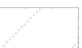
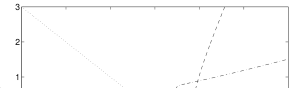
Figure 1: The trajectories of $\phi_{i}$ for $a=i$, $c_{i}=A=-1$ and $m_{\phi_{i}}=100\rm{GeV}$ with dashed line for the first, dash-dotted for the second and dotted for the third family.

For simplicity, we have restricted our considerations to the case where the Yukawa coupling matrix $\lambda_{ij}$ is diagonal. We then find inumerical solutions which are stable. In Figs. 1, 2 we have plotted the trajectories of the scalar fields $\phi_{i}$ in the complex plane. In contrast with the one field case [7, 10], the scalar fields do not relax directly into the origin when $H\ll m_{S}$. This is also implicit in Fig. 3 where there is a non-zero charge for the slepton fields right from the beginning. This feature can be ascribed to a phase oscillation around the minimum of the potential.

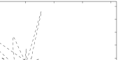
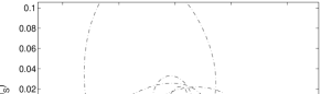
Figure 2: The end trajectories of $\phi_{i}$ for $a=i$, $c_{i}=A=-1$ and $m_{\phi_{i}}=100\rm{GeV}$ with dashed line for the first, dash-dotted for the second and dotted for the third family.

In Fig. 3 we have plotted the evolution of the lepton charge densities in the co-moving volume of the slepton fields $L_{i}$ as parameterized in Eq. (37). Note that the total lepton charge is in units of $m_{\phi}^{2}M_{p}$, where $m_{\phi}=100~{}\rm{GeV}$. The initial conditions were again chosen by first solving the equations of motion during inflation.

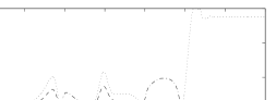
Figure 3: The charge densities in the co-moving volume for the three slepton fields with dashed line for the first, dash-dotted for the second and dotted for the third family. The total slepton charge density is given by the solid line. The parameters were $m_{\phi_{i}}^{2}=1$, $c_{i}=A=-1$, $a=i$ and $\lambda_{ij}=\delta_{ij}$.

In Fig. 4 we have plotted the dependence of charge density against the phase $\theta_{a}$ of Hubble-induced A-term coefficient $a$ with two different initial conditions during inflation. The different initial conditions definitely affect the charge densities of the individual slepton fields. However, although the initial conditions also affect the total charge density, the effect is not as large as for the individual charges. If one where to choose all the initial field values equal so that all the charge densities would be equal, the total charge density evolution would differ from those presented in Fig. 4 in magnitude but not in overall shape.

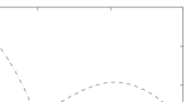
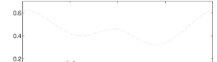
Figure 4: The charge density vs. the phase $\theta_{a}$ of $a$ with initial conditions during inflation $\phi_{1}=1$, $\phi_{2}=i$ and $\phi_{3}=-1$ in the upper figure and $\phi_{1}=1$, $\phi_{2}=i$ and $\phi_{3}=-1+i$ in the lower figure, where field values are in units of $(M_{p}H_{I})^{1/2}$. The initial velocities vanish and the parameter values are $m_{\phi_{i}}^{2}=1$, $c_{i}=A=-1$, $|a|=1$ and $\lambda_{ij}=\delta_{ij}$. Again solid line is for total charge, dashed line for $L_{1}$, dash-dot for $L_{2}$ and dotted for $L_{3}$. In the upper figure $L_{1}$ and $L_{3}$ are actually the same curve.

In Fig. 5 we plot the charge asymmetry $q_{tot}/n_{tot}$, where $q_{tot}=\sum q_{i}$ and $n_{tot}=\sum|q_{i}|$. One sees that for all these cases one produces a charge asymmetry of roughly $\sim 0.1$.

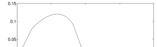
Figure 5: The charge asymmetries related to the cases of fig. 3 with the same parameter values and initial conditions.

7 Conclusions and Discussion

The numerical studies indicate the produced baryon-to-entropy ratio is not significantly changed when including all the lepton families to the $H_{u}L$ flat direction. It thus seems that the simple one-field case captures the essential features of the Affleck-Dine mechanism, at least for $H_{u}L$.

However, there are some interesting details that do change. The first is that the flat direction has non-minimal kinetic terms, which is due to the fact that the sub-manifold spanned by the flat direction is curved. In the one-field case non-minimality is absent because all the one-dimensional manifolds are flat. Hence there is always a choice of coordinates where the field metric is given by just the Kronecker delta. Another difference is that there is phase motion of the fields already right after inflation. This is due to the F-terms containing cross terms that break individual lepton symmetries. However, the F-terms conserve the total lepton charge which is produced only through the A-term. The individual charges may in general have opposite signs and can give substantial contribution to the entropy, which is proportional to the sum of absolute values of the individual charge densities. The total charge is the sum of individual charge densities and thus cancellations can occur.

Although the behaviour of a homogenous $H_{u}L$ background with multiple scalar fields is not qualitatively different from the corresponding one-field case, this may not be true if inhomogeneities are taken into account. For small cosmological perturbations and multiple fields the gauge current condition of Eq. (35) becomes highly non-trivial. This can be seen as follows. $H_{u}L$ is described by three complex scalar fields or six real degrees of freedom. The current condition Eq. (35) defines a two-dimensional submanifold in the six-dimensional space, so that there are four real fluctuation degrees of freedom that would not obey Eq. (35). Hence there would exist matter currents. This implies that the pure gauge field no longer provides a solution for the equations of motion. As a consequence, there would arise electric and magnetic gauge fields which could contribute to the CMB perturbations. These might be of paramount importance for condensate fragmentation, since the fragments (the ground states of which are Q-balls) result from the non-linearities of the perturbations [8, 9]. The Q-ball properties [22] have been considered only for condensates with minimal kinetic terms.

In this paper we focused on the $H_{u}L$ direction. For other directions more complications may arise. For example, the $d=6$ flat direction $(LL)(\bar{d}\bar{d}\bar{d})(\bar{u}\bar{d}\bar{d})$ has six different superpotential terms that contribute to the lifting of the flat direction: $d=4$ term $\bar{u}\bar{u}\bar{d}\bar{e}$, $d=5$ terms $H_{u}L\bar{u}\bar{d}\bar{d}$ and $H_{d}L\bar{d}\bar{d}\bar{d}$ and $d=6$ terms $\bar{u}\bar{d}\bar{d}QL\bar{d}$, $(\bar{u}\bar{d}\bar{d})(\bar{u}\bar{d}\bar{d})$ and $LL\bar{e}\bar{u}\bar{d}\bar{d}$. The $d=5,~{}6$ terms have $B-L=-2$ whereas the $d=4$ term has $B-L=0$. These will give rise to cross terms in the F term which has a non-zero $B-L$ and therefore contributes to the total charge. Such a situation occurs whenever the various superpotential terms with different $B-L$ have at least one field in common.

Acknowledgements

A.J. is supported by Magnus Ehrnrooth foundation. K.E. is supported partly by the Academy of Finland grant no. 75065, and A.M. is a CITA-National fellow. We thank Karsten Jedamzik for helpful discussion.

Appendix A Projection Matrices

Projection of a vector $\mathbf{a}$ along a vector $\mathbf{b}$ is given by

$$\mbox{$$}\mathbf{b}\,\frac{<\mathbf{b}|\mathbf{a}>}{|\mathbf{b}|^{2}}\,,\vspace{\undereqskip}$$ (51)

where $<\cdot|\cdot>$ is a (complex) scalar product. The operation of projection corresponds to a matrix

$$\mbox{$$}P=\frac{\mathbf{b}\mathbf{b}^{\dagger}}{\mathbf{b}^{\dagger}\mathbf{b}}\,,\vspace{\undereqskip}$$ (52)

where we have marked the vector with a column matrix and $\dagger$ represents the hermitian conjugation. Then Eq. (51) is just $P\mathbf{a}$.

In the present paper the projection operators needed are somewhat complicated since in principle they operate on the real basis of complex vectors. Therefore we write complex scalar fields in terms of two real fields $\phi_{i}=\psi_{i}+i\chi_{i}$. Then we can form a vector

$$\mbox{$$}\left(\begin{array}[]{ll}\psi\\ \chi\end{array}\right)\,,\vspace{\undereqskip}$$ (53)

which represents $\phi$ in the real basis. One can change the basis to complex vectors $\phi$ and $\phi^{*}$ with

$$\mbox{$$}\Phi\equiv\left(\begin{array}[]{ll}\phi\\ \phi^{*}\end{array}\right)=\left(\begin{array}[]{ll}1&i\\ 1&-i\end{array}\right)\left(\begin{array}[]{ll}\psi\\ \chi\end{array}\right)\,,\vspace{\undereqskip}$$ (54)

and construct a projection operator

$$\mbox{$$}P_{1}=\frac{\Phi\Phi^{\dagger}}{\Phi^{\dagger}\Phi}\,.\vspace{\undereqskip}$$ (55)

We also need a projection operator along the vector orthogonal to $\Phi$

$$\mbox{$$}P_{2}=\frac{\Psi\Psi^{\dagger}}{\Psi^{\dagger}\Psi}\,,\vspace{\undereqskip}$$ (56)

where

$$\mbox{$$}\Psi=\left(\begin{array}[]{ll}\phi\\ -\phi^{*}\end{array}\right)\,.\vspace{\undereqskip}$$ (57)

It is easy to check that $P_{1}^{2}=P_{1}$, $P_{2}^{2}=P_{2}$ and $P_{1}P_{2}=P_{2}P_{1}=0$. With the help of these projection operators we can form the following combinations

$$\mbox{$$}\Phi^{\dagger}\Phi=\Psi^{\dagger}\Psi=2\sum_{k}|\phi_{k}|^{2}$$

$$\partial_{\mu}\Phi^{\dagger}P_{1}\partial^{\mu}\Phi=\frac{\left[\sum_{j}(\phi_{j}^{*}\partial_{\mu}\phi_{j}+\phi_{j}\partial_{\mu}\phi_{j}^{*})\right]^{2}}{2\sum_{k}|\phi_{k}|^{2}}\,$$

$$\partial_{\mu}\Phi^{\dagger}P_{2}\partial^{\mu}\Phi=\partial_{\mu}\Psi^{\dagger}P_{1}\partial^{\mu}\Psi=-\frac{\left[\sum_{j}(\phi_{j}^{*}\partial_{\mu}\phi_{j}-\phi_{j}\partial_{\mu}\phi_{j}^{*})\right]^{2}}{2\sum_{k}|\phi_{k}|^{2}}\,.\vspace{\undereqskip}$$ (58)

With these identities we can write the Lagrangian as

$$\mbox{$$}\mathcal{L}=\frac{1}{2}\partial_{\mu}\Phi^{\dagger}\left(1+P_{1}-\frac{1}{2}P_{2}\right)\partial^{\mu}\Phi-V(\Phi,\Phi^{\dagger})\,.\vspace{\undereqskip}$$ (59)

The equations of motion read then

$$\mbox{$$}\left(1+P_{1}-\frac{1}{2}P_{2}\right)(\partial_{\mu}\partial^{\mu}\Phi+3H\dot{\Phi})+{{\partial V}\over{\partial\Phi^{\dagger}}}-\partial_{\mu}\Psi\frac{\Psi^{\dagger}\partial^{\mu}\Phi}{\Phi^{\dagger}\Phi}$$

$$+\frac{\Psi}{\Phi^{\dagger}\Phi}\partial_{\mu}\Psi^{\dagger}P_{2}\partial^{\mu}\Phi+\frac{\Phi}{\Phi^{\dagger}\Phi}\partial_{\mu}\Phi^{\dagger}\left(1-P_{1}-\frac{1}{2}P_{2}\right)\partial^{\mu}\Phi=0\,,\vspace{\undereqskip}$$ (60)

where $a$ is the scale factor of the FRW metric.

There is a formula for inverting a unit operator plus a sum of orthogonal projection operators, given by

$$\mbox{$$}\left(1+\sum_{i}a_{i}P_{i}\right)^{-1}=1-\sum_{i}\frac{a_{i}}{1+a_{i}}P_{i},\vspace{\undereqskip}$$ (61)

where $P_{i}P_{j}=\delta_{ij}P_{i}$ and $a_{i}\in\mathbb{C}\backslash\{-1\}$. Using Eq. (61) in Eq. (A), we then obtain a form for the equation of motion which is more easily comparable to the standard case:

$$\mbox{$$}\partial_{\mu}\partial^{\mu}\Phi+3H\dot{\Phi}+\left(1-\frac{1}{2}P_{1}+P_{2}\right){{\partial V}\over{\partial\Phi^{\dagger}}}-\partial_{\mu}\Psi\frac{\Psi^{\dagger}\partial^{\mu}\Phi}{\Phi^{\dagger}\Phi}$$

$$+\frac{\Psi}{\Phi^{\dagger}\Phi}\partial_{\mu}\Psi^{\dagger}P_{2}\partial^{\mu}\Phi+\frac{\Phi}{2\Phi^{\dagger}\Phi}\partial_{\mu}\Psi^{\dagger}\left(1-P_{1}-\frac{3}{2}P_{2}\right)\partial^{\mu}\Phi=0\,.\vspace{\undereqskip}$$ (62)

References

References

- [1]
- [2] F. Buccella, J. P. Derendinger, C. A. Savoy and S. Ferrara, CERN-TH-3212 Presented at 2nd Europhysics Study Conf. on the Unfication of the Fundamental Interactions, Erice, Italy, Oct 6-14, 1981; F. Buccella, J. P. Derendinger, S. Ferrara and C. A. Savoy, Phys. Lett. B 115 (1982) 375.
- [3] M. Grisaru, W. Siegel, and M. Rocek, Nucl. Phys. B 159, 429 (1979); N. Seiberg, Phys. Lett. B 318, 469 (1993). [arXiv:hep-ph/9309335].
- [4] K. Enqvist and A. Mazumdar, Phys. Rept. 380, 99 (2003) [arXiv:hep-ph/0209244].
- [5] I. Affleck and M. Dine, Nucl. Phys. B 249 (1985) 361.
- [6] M. Dine, L. Randall and S. Thomas, Phys. Rev. Lett. 75 (1995) 398 [arXiv:hep-ph/9503303].
- [7] M. Dine, L. Randall and S. Thomas, Nucl. Phys. B 458 (1996) 291 [arXiv:hep-ph/9507453].
- [8] A. Kusenko, Phys. Lett. B 405, 108 (1997) [arXiv:hep-ph/9704273]; A. Kusenko and M. E. Shaposhnikov, Phys. Lett. B 418, 46 (1998) [arXiv:hep-ph/9709492].
- [9] K. Enqvist and J. McDonald, Phys. Lett. B 425, 309 (1998) [arXiv:hep-ph/9711514]; K. Enqvist and J. McDonald, Nucl. Phys. B 538, 321 (1999) [arXiv:hep-ph/9803380].
- [10] A. Jokinen, arXiv:hep-ph/0204086.
- [11] S. Kasuya and M. Kawasaki, Phys. Rev. D 61 (2000) 041301 [arXiv:hep-ph/9909509]; S. Kasuya and M. Kawasaki, Phys. Rev. D 62 (2000) 023512 [arXiv:hep-ph/0002285]; K. Enqvist, A. Jokinen and J. McDonald, Phys. Lett. B 483 (2000) 191 [arXiv:hep-ph/0004050]; K. Enqvist, A. Jokinen, T. Multamaki and I. Vilja, Phys. Rev. D 63, 083501 (2001) [arXiv:hep-ph/0011134]; S. Kasuya and M. Kawasaki, Phys. Rev. D 64 (2001) 123515 [arXiv:hep-ph/0106119]; T. Multamaki and I. Vilja, Phys. Lett. B 535 (2002) 170 [arXiv:hep-ph/0203195].
- [12] K. Enqvist, S. Kasuya and A. Mazumdar, Phys. Rev. Lett. 89, 091301 (2002) [arXiv:hep-ph/0204270]. K. Enqvist, S. Kasuya and A. Mazumdar, Phys. Rev. D 66, 043505 (2002) [arXiv:hep-ph/0206272].
- [13] K. Enqvist and J. McDonald, Phys. Rev. Lett. 83, 2510 (1999) [arXiv:hep-ph/9811412]. K. Enqvist and J. McDonald, Phys. Rev. D 62, 043502 (2000) [arXiv:hep-ph/9912478]. M. Kawasaki and F. Takahashi, Phys. Lett. B 516, 388 (2001) [arXiv:hep-ph/0105134].
- [14] K. Enqvist, S. Kasuya and A. Mazumdar, Phys. Rev. Lett. 90, 091302 (2003) [arXiv:hep-ph/0211147]; M. Postma, Phys. Rev. D 67, 063518 (2003) [arXiv:hep-ph/0212005]; K. Enqvist, A. Jokinen, S. Kasuya and A. Mazumdar, arXiv:hep-ph/0303165; S. Kasuya, M. Kawasaki and F. Takahashi, arXiv:hep-ph/0305134; M. Postma and A. Mazumdar, arXiv:hep-ph/0304246; K. Hamaguchi, M. Kawasaki, T. Moroi and F. Takahashi, arXiv:hep-ph/0308174; K. Enqvist, S. Kasuya and A. Mazumdar, arXiv:hep-ph/0311224.
- [15] K. Enqvist, A. Mazumdar and M. Postma, Phys. Rev. D 67, 121303 (2003) [arXiv:astro-ph/0304187]; A. Mazumdar and M. Postma, Phys. Lett. B 573, 5 (2003) [arXiv:astro-ph/0306509].
- [16] T. Gherghetta, C. F. Kolda and S. P. Martin, model,” Nucl. Phys. B 468 (1996) 37 [arXiv:hep-ph/9510370].
- [17] M. Senami and K. Yamamoto, Phys. Lett. B 524 (2002) 332 [arXiv:hep-ph/0105054]; M. Senami and K. Yamamoto, Phys. Rev. D 66 (2002) 035006 [arXiv:hep-ph/0205041]; M. Senami and K. Yamamoto, Phys. Rev. D 67 (2003) 095005 [arXiv:hep-ph/0210073]; M. Senami and K. Yamamoto, arXiv:hep-ph/0305202;
- [18] H. P. Nilles, Phys. Rept. 110 (1984) 1.
- [19] G. Sartori, J. Math. Phys. 24 (1983) 765; R. Gatto and G. Sartori, Phys. Lett. B 118 (1982) 79; C. Procesi and G. W. Schwarz, Phys. Lett. B 161 (1985) 117; R. Gatto and G. Sartori, Phys. Lett. B 157 (1985) 389; R. Gatto and G. Sartori, Commun. Math. Phys. 109 (1987) 327; G. Sartori, Mod. Phys. Lett. A 4 (1989) 91.
- [20] P. Brax and C. A. Savoy, arXiv:hep-th/0104077.
- [21] C. F. Kolda and J. March-Russell, Phys. Rev. D 60 (1999) 023504 [arXiv:hep-ph/9802358].
- [22] S. R. Coleman, Nucl. Phys. B 262 (1985) 263 [Erratum-ibid. B 269 (1986) 744].