OITS-742

Flavor and CP violating $Z$ exchange and the rate asymmetry in $B\to\phi K_{S}$
N.G. Deshpande and Dilip Kumar Ghosh

Institute of Theoretical Science

University of Oregon, Eugene, OR 97403

Recent measurements of time dependent CP asymmetry in $B\to\phi K_{S}$, if confirmed, would indicate a new source of CP violation. We examine flavor violating tree-level $Z$ currents in models with extra down-type quark singlets that arise naturally in string compactified gauge groups like $E_{6}$. We evaluate the new operators at the scale $\mu\approx{\cal O}(m_{b})$ in NLO, and using QCD improved factorization to describe $B\to\phi K_{S}$, find the allowed range of parameters for $\rho$ and $\psi$, the magnitude and phase of the flavor violating parameter $U_{bs}$. This allowed range does satisfy the constraint from flavor changing process $b\to s\ell^{+}\ell^{-}$. However, further improvement in measurement of these rates could severely constrain the model.

1 Introduction

The ongoing $B$ physics experiments by BaBar and Belle collaborations  [1, 2] provide a unique opportunity to study the flavor structure of the standard model quark sector and also the origin of CP violation. In addition to this, any new physics effects in $B$ physics can also be tested in these experiments. Recent time dependent asymmetries measured in the decay $B\to\phi K_{S}$ both by BaBar and Belle collaborations [References-References] show significant deviation from the standard model and this has generated much theoretical speculation regarding physics beyond the standard model [5]. In the standard model, the process $B\to\phi K_{S}$ is purely penguin dominated and the leading contribution has no weak phase. The coefficient of $\sin(\Delta m_{B}t)$ in the asymmetry therefore should measure $\sin 2\beta$, the same quantity that is involved in $B\to\psi K_{S}$ in the standard model. The most recent measured average values of asymmetries are  [4, 6] $S_{\psi K_{S}}=0.734\pm 0.055$ and $S_{\phi K_{S}}=-0.15\pm 0.33$. The value for $S_{\psi K_{S}}$ agrees with the standard model expectation. The deviation in the $\phi K_{S}$ is intriguing because a penguin process being a loop induced process is particularly sensitive to new physics which can manifest itself through exchange of heavy particles. In this article we will consider an extension of the standard model, with extra down type singlet quarks. These extra down type singlet quarks appear naturally in each 27-plet fermion generation of $E_{6}$ Grand Unification Theories (GUTs) [References-References]. The mixing of these singlet quarks with with the three SM down type quarks, provides a framework to study the deviations from the unitarity constraints of $3\times 3$ CKM matrix. This model has been previously studied in connection with $R_{b}$ and F-B asymmetry at the $Z$ pole as it provides a framework for violation of the unitarity of the CKM matrix [References-References]. This mixing also induces tree-level flavor changing neutral currents (FCNC). These tree-level FCNC couplings can have a significant effects on different $CP$ conserving as well as CP violating B processes [References, References - References].

In this article we study the FCNC effect arising from the $Z-b-\bar{s}$ coupling $U_{bs}$ to the $B\to\phi K_{S}$ process. This new FCNC coupling $U_{bs}$ can have a phase, which can generate the additional source of CP violation in the $B\to\phi K_{S}$ process, and thus affect measured values of $S_{\phi K_{S}}$ and $C_{\phi K_{S}}$. We parameterize this coupling by $U_{bs}=\rho e^{i\psi}$. We then study $B\to\phi K_{S}$ taking into account the new interactions in the QCD improved factorization scheme (BBNS approach ) [25]. This method incorporates elements of naive factorization approach (as its leading term ) and perturbative QCD corrections (as sub-leading contributions) and allows one to compute systematic radiative corrections to the naive factorization for the hadronic $B$ decays. Recently, several studies of $B\to PV$, and specifically $B\to\phi K_{S}$ have been performed within the frame work of QCD improved factorization scheme [References-References]. In our analysis of $B\to\phi K_{S}$, we follow [30] which is based on the original paper [25]. In our analysis, we only consider the contribution of the leading twist meson wave functions, and also neglect the weak annihilation contribution which is expected to be small. Inclusion of these would introduce more model dependence in the calculation through the parameterization of an integral, which is otherwise infrared divergent.

The time dependent CP asymmetry of $B\to\phi K_{S}$ is described by :

$${\cal A}_{\phi K_{S}}(t) = \frac{\Gamma(\overline{B^{0}}(t)\to\phi K_{S})-\Gamma(B^{0}(t)\to\phi K_{S})}{\Gamma(\overline{B^{0}}(t)\to\phi K_{S})+\Gamma(B^{0}(t)\to\phi K_{S})}$$ (1)

$$= -C_{\phi K_{S}}\cos(\Delta m_{B}t)+S_{\phi K_{S}}\sin(\Delta m_{B}t)$$ (2)

where $S_{\phi K_{S}}$ and $C_{\phi K_{S}}$ are given by

$$S_{\phi K_{S}}=\frac{2Im~{}\lambda_{\phi K_{S}}}{1+\mid\lambda_{\phi K_{S}}\mid^{2}},~{}~{}~{}~{}C_{\phi K_{S}}=\frac{1-\mid\lambda_{\phi K_{S}}\mid^{2}}{1+\mid\lambda_{\phi K_{S}}\mid^{2}}$$ (3)

and $\lambda_{\phi K_{S}}$ can be expressed in terms of decay amplitudes:

$$\lambda_{\phi K_{S}}=-e^{-2i\beta}\frac{{\overline{\cal M}}(\overline{B^{0}}\to\phi K_{S})}{{\cal M}(B^{0}\to\phi K_{S})}$$ (4)

The branching ratio and the direct CP asymmetries of both the charged and neutral modes of $B\to\phi K_{S}$ have been measured [1, 2, 3, 4, 6, 31]

$${\cal B}(B^{0}\to\phi K_{S}) = (8.0\pm 1.3)\times 10^{-6}$$ (5)

$${\cal B}(B^{+}\to\phi K^{+}) = (9.4\pm 0.9)\times 10^{-6},$$ (6)

$$S_{\phi K_{S}} = +0.45\pm 0.43\pm 0.07~{}~{}(\rm{BaBar});$$ (7)

$$= -0.96\pm 0.50^{+0.09}_{-0.11}~{}~{}({\rm Belle});$$ (8)

$$= -0.15\pm 0.33~{}~{}({\rm World~{}average});$$ (9)

$$C_{\phi K_{S}} = -0.19\pm 0.30$$ (10)

$${\cal A}_{CP}(B^{+}\to\phi K^{+}) = (3.9\pm 8.8\pm 1.1)\%$$ (11)

scale	$C_{1}$	$C_{2}$	$C_{3}$	$C_{4}$	$C_{5}$	$C_{6}$
$\mu=m_{b}/2$	1.137	-0.295	0.021	-0.051	0.010	-0.065
$\mu=m_{b}$	1.081	-0.190	0.014	-0.036	0.009	-0.042
	$C_{7}/\alpha_{em}$	$C_{8}/\alpha_{em}$	$C_{9}/\alpha_{em}$	$C_{10}/\alpha_{em}$	$C_{7\gamma}$	$C_{8g}$
$\mu=m_{b}/2$	-0.024	0.096	-1.325	0.331	-0.364	-0.169
$\mu=m_{b}$	-0.011	0.060	-1.254	0.223	-0.318	-0.151

Table 1: Standard model Wilson coefficients in NDR scheme.

2 $B\to\phi K_{S}$ in the QCDF Approach

In the standard model, the effective Hamiltonian for charmless $B\to\phi K_{S}$ decay is given by [25]

$${\cal H}_{eff}=-\frac{G_{F}}{\sqrt{2}}V_{tb}V^{\ast}_{ts}\left[C_{1}(\mu){\cal O}_{1}(\mu)+C_{2}(\mu){\cal O}_{2}(\mu)+\sum^{10}_{i=3}C_{i}(\mu){\cal O}_{i}(\mu)+C_{7\gamma}{\cal O}_{7\gamma}+C_{8g}{\cal O}_{8g}\right]$$ (12)

where the Wilson coefficients $C_{i}(\mu)$ are obtained from the weak scale down to scale $\mu$ by running the renormalization group equations. The definitions of the operators can be found in Ref.[25]. The Wilson coefficients $C_{i}$ can be computed using different schemes [35]. In this paper we will use the NDR scheme. The NLO values of $C_{i}(i=1-10)$ and LO values of $C_{7\gamma},C_{8g}$ respectively at $\mu=m_{b}/2$ and $m_{b}$ used by us based on Ref.[25] are shown in Table 1.

In the QCD improved factorization scheme, the $B\to\phi K_{S}$ decay amplitude due to a particular operator can be represented in following form :

$$<\phi K\mid{\cal O}\mid B>=<\phi K\mid{\cal O}\mid B>_{fact}\left[1+\sum r_{n}\alpha_{s}^{n}+O(\Lambda_{QCD}/m_{b})\right]$$ (13)

where $<\phi K\mid{\cal O}\mid B>_{fact}$ denotes the naive factorization result.The second and third term in the bracket represent higher order $\alpha_{s}$ and $\Lambda_{QCD}/m_{b}$ correction to the hadronic transition amplitude. Following the scheme and notations presented in Ref.[30], we write down the total $B\to\phi K_{S}$ amplitude, which is the sum of the standard model as well as $Z$ exchange tree-level contribution from extra down-type quark singlets (EDQS) model in the heavy quark limit

$${\cal M}(B^{+}\to\phi K^{+}) =$$

$${\cal M}(B^{0}\to\phi K^{0}) = \frac{G_{F}}{\sqrt{2}}m_{B}^{2}f_{\phi}F_{1}^{B\to K}(m^{2}_{\phi})V_{pb}V^{\ast}_{ps}\left[a^{p}_{3}+a^{p}_{4}+a^{p}_{5}\right.$$ (14)

$$\left.-\frac{(a^{p}_{7}+a^{p}_{9}+a^{p}_{10})}{2}+a^{p}_{10a}\right]$$

where $p$ is summed over $u$ and $c$. The coefficients $a^{p}_{i}$ are given by

$$a^{u}_{3}=a^{c}_{3}=C^{\prime}_{3}+{C^{\prime}_{4}\over N_{c}}\left[1+{C_{F}\alpha_{s}\over 4\pi}\left(V_{\phi}+H_{\phi}\right)\right],$$

$$a^{p}_{4}=C^{\prime}_{4}+{C^{\prime}_{3}\over N_{c}}\left[1+{C_{F}\alpha_{s}\over 4\pi}\left(V_{\phi}+H_{\phi}\right)\right]+{C_{F}\alpha_{s}\over 4\pi N_{c}}P^{p}_{\phi},$$

$$a^{u}_{5}=a^{c}_{5}=C^{\prime}_{5}+{C^{\prime}_{6}\over N_{c}}\left[1+{C_{F}\alpha_{s}\over 4\pi}(-12-V_{\phi})\right],$$

$$a^{u}_{7}=a^{c}_{7}=C^{\prime}_{7}+{C^{\prime}_{8}\over N_{c}}\left[1+{C_{F}\alpha_{s}\over 4\pi}(-12-V_{\phi}-H_{\phi})\right],$$

$$a^{u}_{9}=a^{c}_{9}=C^{\prime}_{9}+{C^{\prime}_{10}\over N_{c}}\left[1+{C_{F}\alpha_{s}\over 4\pi}\left(V_{\phi}+H_{\phi}\right)\right],$$

$$a^{u}_{10}=a^{c}_{10}=C^{\prime}_{10}+{C^{\prime}_{9}\over N_{c}}\left[1+{C_{F}\alpha_{s}\over 4\pi}\left(V_{\phi}+H_{\phi}\right)\right],$$

$$a^{p}_{10}={C_{F}\alpha_{s}\over 4\pi N_{c}}Q^{p}_{\phi}$$

$$a^{u}_{10a}=a^{c}_{10a}={C_{F}\alpha_{s}\over 4\pi N_{c}}Q_{\phi}$$ (15)

with $C_{F}=(N^{2}_{c}-1)/2N_{c}$ and $N_{c}=3$. The effective Wilson coefficients $C^{\prime}_{i}=C_{i}+\tilde{C}_{i},~{}~{}~{}(i=3-10)$ is the sum of the standard model and the EDQS model Wilson coefficients. The quantities $V_{\phi},H_{\phi},P^{p}_{\phi}$ and $Q^{p}_{\phi}$ are hadronic parameters that contain all nonperturbative dynamics, are given in Ref. [25, 36].

For the sake of completeness, we give the branching ratio for $B\to\phi K_{S}$ decay channel in the rest frame of the $B$ meson.

$${\cal BR}(B\to\phi K_{S})=\frac{\tau_{B}}{8\pi}\frac{\mid P_{cm}\mid}{m^{2}_{B}}\mid{\cal M}(B\to\phi K_{S})\mid^{2}$$ (16)

where, $\tau_{B}$ represents the $B$ meson lifetime and the kinematical factor $\mid P_{cm}\mid$ is written as

$$\mid P_{cm}\mid=\frac{1}{2m_{B}}\sqrt{\left[m^{2}_{B}-(m_{K}+m_{\phi})^{2}\right]\left[m^{2}_{B}-(m_{K}-m_{\phi})^{2}\right]}$$ (17)

3 FCNC $Z$ couplings in EDQS model

Models with extra down-type quarks (EDQS) have a long history. The earliest consideration of such models was in the context of the grand unification group $E_{6}$ which arises from string compactification. The quarks and leptons of each generation belong to the $27$ representation [References-References]. Each generation has one extra quark singlet of the down type, and also one extra lepton of the electron type. The group also has extra $Z$ bosons, which we will assume to be too heavy to have any effect on $B\to\phi K_{S}$ process. The down type mass matrix is then a $6\times 6$ by-unitary matrix, and in general when we rotate the quarks to their mass basis, off-diagonal couplings arise. In EDQS model, the $Z$ mediated FCNC interactions are given by

$${\cal L}=\frac{g}{2\cos\theta_{W}}\left[\bar{d}_{L\alpha}U_{\alpha\beta}\gamma^{\mu}d_{L\beta}\right]Z_{\mu}$$ (18)

In general for $n$ copies of extra down-type quark singlet model, $U_{\alpha\beta}$ is :

$$U_{\alpha\beta}=\sum^{3}_{i=1}V^{\dagger}_{\alpha i}V_{i\beta}=\delta_{\alpha\beta}-\sum^{N_{d}}_{i=4}V^{\dagger}_{\alpha i}V_{i\beta},~{}~{}~{}~{}~{}(\alpha,\beta=d,s,b,B_{1},B_{2}....)$$ (19)

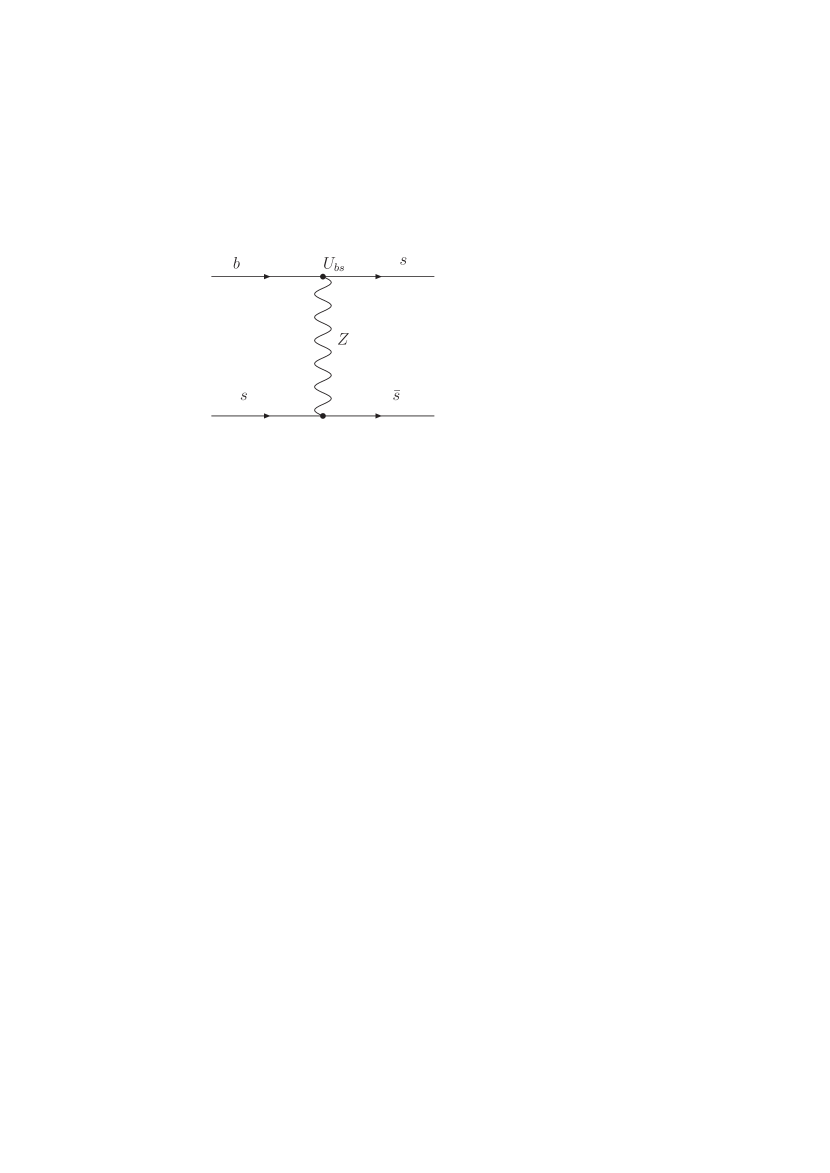
Figure 1: Feynman diagram for $Z$ exchange tree-level contribution to $b\to ss\bar{s}$ process.

where, $N_{d}=3+n$ represents the number of down type quark states, and $U$ is the neutral current mixing matrix for the down quark sector. The non vanishing components of $U_{\alpha\beta}$ will lead to FCNC process at tree level, generating new physics contribution to the measured CP asymmetries. The new tree level FCNC $Z$ mediated contribution to the $b\to sq\bar{q}$ process is shown in Figure 1. The new operators arising from this tree-level FCNC process have been shown to lead to the following effective Hamiltonian for $b\to sq\bar{q}$ process in this model  [22]:

$${\cal H}^{new}_{Z} = -\frac{G_{F}}{\sqrt{2}}V_{tb}V^{*}_{ts}\left[\tilde{C}_{3}{\cal O}_{3}+\tilde{C}_{7}{\cal O}_{7}+\tilde{C}_{9}{\cal O}_{9}\right]$$ (20)

where, the new Wilson coefficients $\tilde{C}_{3},\tilde{C}_{7}$ and $\tilde{C}_{9}$ at the scale $M_{Z}$ are given by:

$$\tilde{C}_{3}(M_{Z}) = \frac{\kappa}{6},$$ (21)

$$\tilde{C}_{7}(M_{Z}) = \kappa\frac{2}{3}\sin^{2}\theta_{W},$$ (22)

$$\tilde{C}_{9}(M_{Z}) = -\kappa\frac{2}{3}\left(1-\sin^{2}\theta_{W}\right)$$ (23)

where, $\kappa=\frac{U_{bs}}{(V_{tb}V^{*}_{ts})}$, and operators ${\cal O}_{i}$ in Eq. (20) are given in Ref.[25]. We now evolve these new Wilson coefficients from the scale $M_{Z}$ to the scale $\mu\approx{\cal O}(m_{b})$ using the renormalization group equation. While doing this we have considered NLO QCD correction [37], neglecting the order $\alpha$ electroweak contributions to the RG evolution equation which are tiny. At the low energy, after the RG evolution the above three Wilson coefficients $(\tilde{C}_{3},\tilde{C}_{7},\tilde{C}_{9})$ generate new set of Wilson coefficients $(\tilde{C}_{i},i=3-10)$ in this model. The values of Wilson coefficients ( without taking the overall factor $\kappa$) at scales $\mu=(m_{b}/2,m_{b})$ are shown in Table 2.

scale	$\tilde{C}_{3}$	$\tilde{C}_{4}$	$\tilde{C}_{5}$	$\tilde{C}_{6}$	$\tilde{C}_{7}$	$\tilde{C}_{8}$	$\tilde{C}_{9}$	$\tilde{C}_{10}$
$\mu=m_{b}/2$	0.195	-0.088	0.0180	-0.053	0.133	0.108	-0.604	0.174
$\mu=mb$	0.182	-0.0629	0.0157	-0.0370	0.136	0.0732	-0.574	0.122

Table 2: Wilson coefficients of EDQS model in NDR scheme, without the overall multiplicative factor $\kappa$.

4 $B$ physics constraints on $U_{bs}$

In this section, we review the constraints on the flavor violating parameter $U_{bs}$ from different flavor changing $B$ processes. These processes can be classified into two classes, CP conserving and CP violating. Among the CP conserving processes, ${\cal B}(B\to X_{s}\ell^{+}\ell^{-})$, and $\Delta M_{B_{s}}$ can put constraints on $U_{bs}$ [13, 15, 16]. Using recent Belle [38] measurement of ${\cal B}(B\to X_{s}\ell^{+}\ell^{-})=(6.1\pm 1.4^{+1.4}_{-1.1})\times 10^{-6}$ the authors in Ref.[21] had shown that $\mid U_{bs}\mid\leq 1\times 10^{-3}$. However, this bound has recently been updated in Ref.[22] to

$$\mid U_{bs}-4.0\times 10^{-4}\mid\leq 8\times 10^{-4}$$ (24)

which also updates their previous bounds in Ref.[17, 39] The bound in Eq. (24) is based on inclusive $B\to X_{s}e^{+}e^{-}$ decays at NNLO [40]. We shall adopt this bound in our analysis. This bound is valid in both general $n$ extra down-type singlet quark model and in the model with a single extra down-type quark singlet [16]. Similarly, the $b\to s\gamma$ branching ratio provides comparable limits [14, 16].

It has been shown in Ref. [20, 41] that in the presence of tree-level FCNC coupling $U_{bd}$ and /or $U_{bs}$, the standard box diagram for $B_{d/s}-\bar{B}_{d/s}$ is not gauge invariant by itself, but requires $Z$ exchange penguin diagram as well as tree level $Z$ FCNC diagram. The additional Feynman diagrams are given in Ref. [41]. Following the paper [20], with slight change in the notations, we write down the expression for the $B_{q}-\bar{B}_{q}$ mixing:

$$\Delta M_{B_{q}}=\frac{G^{2}_{F}M^{2}_{W}f^{2}_{B_{q}}{\hat{B}}_{B_{q}}m_{B^{0}_{q}}}{6\pi^{2}}\left[\left(\lambda^{t}_{qb}\right)^{2}\eta^{B_{s}}_{tt}S_{0}(x_{t})+\Delta_{new}\right]$$ (25)

where, $(q=d,s)$ and

$$\Delta_{new}=-8U_{bq}\lambda^{t}_{qb}\eta^{B_{q}}_{tt}Y_{0}(x_{t})+\frac{4\pi\sin^{2}\theta_{W}}{\alpha}\eta^{B_{q}}_{Z}U^{2}_{bq}$$ (26)

where, the definitions of different parameters used above can be found in Ref.[20].

We have found that to satisfy the measured $\Delta M_{B_{d}}$ within one sigma, where we consider both the theory error of $20\%$ arising from the value of $f^{2}_{B_{q}}{\hat{B}}_{B_{q}}$ and the experimental error taken in quadrature, the FCNC coupling $\mid U_{bd}\mid$ should be less than $\sim(2-3)\times 10^{-4}$. This is a very stringent limit.

The $\Delta M_{B_{s}}$ has not been measured yet, and so only lower limit on the mass difference is available. We have found that the new contribution to $\Delta M_{B_{s}}$ from EDQS model is less than $3\%$ when compared to the standard model. It can be shown that for similar values of $U_{bd}$ and $U_{bs}$, the FCNC effects on $\Delta M_{B_{s}}$ will be suppressed by a factor $\sim\lambda^{2}$ when compared with the effects on $\Delta M_{B_{d}}$. This implies that in EDQS model, FCNC effects are hard to detect in $B_{s}-\bar{B}_{s}$ mixing [41].

5 $B\to\phi K_{S}$ analysis

In the last section we have discussed the allowed range of the FCNC parameter $U_{bs}$ from different $B$ processes. In this section we will study the effect of this FCNC parameter $(U_{bs})$ in the $B\to\phi K_{S}$ process. For this we express $U_{bs}$ in the following form: $U_{bs}=\rho e^{i\psi}$. We will then vary $\rho$ and $\psi$  in range such that Eq. (24) is satisfied. We then study the allowed region of parameters in the $\rho-\psi$ plane from the three measured quantities $(a)$ ${\cal B}(B\to\phi K_{S})$, $(b)$ $S_{\phi K_{S}}$ and $(c)$ $C_{\phi K_{S}}$. To get the allowed parameter space, from the ${\cal B}(B\to\phi K_{S})$ branching ratio, we allow it to vary by $2\sigma$ respectively from its central value. This $2\sigma$ band contains both experimental and theoretical errors. The main source of theoretical error is the form factor $F^{B\to K}_{1}$. In our analysis we have considered $20\%$ error on this parameter. Similarly, we vary $C_{\phi K_{S}}$ and $S_{\phi K_{S}}$ by $1\sigma$ and $2\sigma$ from their central value to get the allowed region in the $\rho-\psi$ plane.

In Figure $2~{}(a)$ we show such allowed region in $\rho-\psi$ plane for the scale $\mu=m_{b}/2$. The whole area left of the dotted contour is allowed by saturating Eq. (24). The area outside the thick contour labeled by BR is $2\sigma$ allowed region from the branching ratio measurement. The parameter space enclosed by the thin contour marked by $S_{\phi K}$ is allowed by $2\sigma$ from data on the $S_{\phi K_{S}}$. This whole parameter space is allowed by $1\sigma$ from $C_{\phi K_{S}}$ measurement, The regions (marked by $Z$) is the only allowed parameter space in $\rho-\psi$ plane with $6.5\times 10^{-4}\leq\rho\leq 10\times 10^{-4}$ and $-1.7\leq\psi\leq-0.85$ which satisfy the experimentally measured $C_{\phi K_{S}}$, $S_{\phi K_{S}}$ and ${\cal B}(B\to\phi K_{S})$ within the errors described above. We note that only negative values of $\psi$ give acceptable range of $S_{\phi K}$. The Figure $2~{}(b)$ correspond to the scale $\mu=m_{b}$. In this case though we have larger allowed area from the $S_{\phi K}$ measurement, but the $2\sigma$ branching ratio contour pushes the allowed range towards higher values of $\rho$ and somewhat lower range of the phase $\psi$. This particular behavior of the branching ratio contour can be understood from that fact that for $\mu=m_{b}$, the SM branching ratio is $3.8\times 10^{-6}$, which is much smaller than the lower end of the $2\sigma$ band of the experimental number. Hence, one needs larger values of $\rho$ to push the total branching ratio within the $2\sigma$ limit. For this reason the allowed region shrinks to a point in this case.

6 Conclusions

In this paper, we have studied the tree-level flavor violating $Z$ contribution to $B\to\phi K_{S}$ process in models with extra down-type quark singlets which arise naturally in the context of the Grand Unification group $E_{6}$. In the presence of such flavor violating interactions, $B\to\phi K_{S}$ process receives additional contributions, governed by a set of new operators which can be expressed in terms of the standard operators ${\cal O}_{i},(i=3-10)$. We then evolved these new Wilson coefficients from the scale $M_{Z}$ to the scale $\mu={\cal O}(m_{b})$ relevant for our process using the renormalization group equation. We have found that, at the lower scale these Wilson coefficients significantly modified from their initial values at the scale $\mu=M_{Z}$. We have found that this new flavor violating interaction can modify the standard model Wilson coefficients $C_{i},(i=3-10)$ significantly. We have used following experimentally measured quantities: $S_{\phi K_{S}},C_{\phi K_{S}}$ and ${\cal B}(B\to\phi K_{S})$ to constrain the flavor violating parameter $U_{bs}$. We have shown that in the model with an arbitrary number of down type singlet quarks, the value of $S_{\phi K_{S}}$ and $C_{\phi K_{S}}$ can be well explained by the values of $\rho$ and $\psi$ in the region marked by $Z$ in Figure $2~{}(a)$. Improvements in measurements of $B\to X_{s}\ell^{+}\ell^{-}$ can tighten the constraints in Eq. (24) and either rule in or rule out this model.

Acknowledgments

This work was supported in part by US DOE contract numbers DE-FG03-96ER40969. We would like to thank A. K. Giri for helpful correspondence. We would particularly like to thank G. Hiller for clarifying the operator structure of the $Z$ mediated FCNC interactions.

7 APPENDIX : Input parameters and different form factors

In this Appendix we list all the input parameters, decay constants and form factors used for the calculation of $B\to\phi K_{S}$.

1. Coupling constants and masses ( in units of GeV ):
   $\alpha_{em}=1/129,~{}~{}~{}~{}\alpha_{s}(M_{Z})=0.118,~{}~{}~{}~{}G_{F}=1.16639\times 10^{-5}~{}{\rm(GeV)^{-2}},\\ M_{Z}=91.19,~{}~{}~{}~{}m_{b}=4.88,~{}~{}~{}~{}m_{B}=5.2787,\\ ~{}~{}~{}~{}m_{\phi}=1.019,~{}~{}~{}~{}m_{K}=0.493$

2. Wolfenstein parameters :
   $\lambda=0.2205,~{}~{}~{}~{}A=0.815,~{}~{}~{}~{}\eta=0.324,~{}~{}~{}~{}\rho=0.224,~{}~{}~{}~{}$

3. Constituent quark masses $m_{i}(i=u,d,s,c,d)$( in units of GeV):
   $m_{u}=0.2,~{}~{}~{}~{}m_{d}=0.2,~{}~{}~{}~{}m_{s}=0.5,~{}~{}~{}~{}m_{c}=1.5,~{}~{}~{}~{}m_{b}=4.88.$

4. The decay constants (in units of GeV):
   $f_{B}=0.19,~{}~{}~{}~{}f_{\phi}=0.237,~{}~{}~{}~{}f_{K}=0.16$

5. The form factors at zero momentum transfer :
   $F_{1}^{B\to K}=0.33.$

Figure 2: Contour plots of $S_{\phi K_{S}}$, ${\cal B}(B\to\phi K_{S})$ and $\mid U_{bs}-4\times 10^{-4}\mid=8\times 10^{-4}$ in $\rho-\psi$ plane for two values of $\mu=\frac{m_{b}}{2}$ $(a)$ and $m_{b}$ $(b)$ respectively. The area leftside of the dotted contour is the allowed region of $U_{bs}$ from the inclusive $B\to X_{s}\ell^{+}\ell^{-}$ process. In figure $(a)$, the area marked by $Z$ is the $2\sigma$ allowed regions from the measurement of $S_{\phi K}$ and ${\cal B}(B\to\phi K_{S})$. In figure $(b)$, such $2\sigma$ allowed region is a point where the three curves intersect.

References

- [1] B. Aubert et al.[BaBar Collaboration], arXiv:hep-ex/0207070.
- [2] K. Abe et al.[Belle Collaboration], arXiv:hep-ex/0207098
- [3] K. Abe et al.[Belle Collaboration], Phys. Rev. D 67, 031102 (2003) .
- [4] G. Hamel De Monchenault, arXiv:hep-ex/0305055.
- [5] A. Kagan, arXiv:hep-ph/9806266; talk at the 2nd International Workshop on B physics and CP Violation, Taipei, 2002; SLAC Summer Institute on Particle Physics, August 2002; G. Hiller, Phys. Rev. D 66, 071502 (2002) ; A. Datta, Phys. Rev. D 66, 071702 (2002) ; M.Ciuchini and L. Silvestrini, Phys. Rev. Lett. 89, 231802 (2002); B. Dutta, C.S. Kim and S. Oh, Phys. Rev. Lett. 90, 011801 (2003); S. Khalil and E. Kou, Phys. Rev. D 67, 055009 (2003) ; C.W. Chiang and J.L. Rosner, Phys. Rev. D 68, 014007 (2003) ; A. Kundu and T. Mitra, Phys. Rev. D 67, 116005 (2003) ; K. Agashe and C.D. Carone, arXive: hep-ph/0304229; G.L. Kane, P. Ko, H. b. Wang, C. Kolda, J.h. Park and L.T. Wang, Phys. Rev. Lett. 90, 141803 (2003); D. Chakraverty, E. Gabrielli, K. Huitu and S. Khalil, arXiv:hep-ph/0306076; J.F. Cheng, C.S.Huang and X.h. Wu, arXiv: hep-ph/0306086; R. Arnowitt, B. Dutta and B. Hu, arXiv:hep-ph/0307152; C. Dariescu, M. A. Dariescu, N.G. Deshpande and D. K. Ghosh, hep-ph/0308305.
- [6] K. Abe et al.[Belle Collaboration], arXiv:hep-ex/0308035; T. Browder, CKM Phases (), Talk presented at Lepton-Photon 2003.
- [7] F. Gursey, P. Ramond and P. Sikivie, Phys. Lett. B60, 177 (1976) ; Y. Achiman and B. Stech, Phys. Lett. B77, 389 (1978) ; M.J. Bowick and P. Ramond, Phys. Lett. B103, 338 (1981) ; F. del Aguila and M.J. Bowick, Nucl. Phys. B224, 107 (1983) ; J. L. Rosner, Comm.Nucl.Part.Phys. 15,195 (1986).
- [8] V. Barger, N. G. Deshpande, R.J.N. Phillips and K. Whisnant, Phys. Rev. D 33, 1912 (1986) ; V. Barger, R.J.N. Phillips and K. Whisnant, Phys. Rev. Lett. 57, 48 (1986) .
- [9] T. G. Rizzo, Phys. Rev. D 34, 1438 (1986) ; J. L. Hewett, T. G. Rizzo, Z. Phys. C34, 49 (1987) ; Phys. Rep. 183, 193 (1989) .
- [10] V. Barger, M. S. Berger and R.J.N. Phillips, Phys. Rev. D 52, 1663 (1995) .
- [11] F. del Aguila and J. Cortes, Phys. Lett. B156, 243 (1985) ; G.C. Branco and L. Lavoura, Nucl. Phys. B278, 238 (1986) ; F. del Aguila, M. K. Chase and J. Cortes, Nucl. Phys. B271, 61 (1986) ; Y. Nir and D. J. Silverman, Phys. Rev. D 42, 1477 (1990) ; D. Silverman, Phys. Rev. D 45, 1800 (1992) ; G.C.Branco, T. Morozumi, P. A. Parada and M.N. Rebelo, Phys. Rev. D 48, 1167 (1993) ; D. Silverman, Int. J. Mod. Phys. A11, 2253 (1996) ; Phys. Rev. D 58, 095006 (1998) ; M. Gronau and D. London, Phys. Rev. D 55, 2845 (1997) ; F. del Aguila, J. A. Aguilar-Saavedra and G. C. Branco, Nucl. Phys. B510, 39 (1998) .
- [12] F.del Aguila, J. A. Aguilar-Saavedra and R. Miquel, Phys. Rev. Lett. 82, 1628 (1999) .
- [13] M.R. Ahmady, M. Nagashima and A. Sugamoto, hep-ph/0105049.
- [14] C.V. Chang, D. Chang and W. Keung, Phys. Rev. D 61, 053007 (2000) ; M. Aoki, E. Asakawa, M. Nagashima, N. Oshimo and A. Sugamoto, Phys. Lett. B487, 321 (2000).
- [15] G. Barenboim, F.J. Botella and O. Vives, Phys. Rev. D 64, 015007 (2001) .
- [16] G. Barenboim, F.J. Botella and O. Vives, Nucl. Phys. B, 613,285 (2001)
- [17] G. Buchalla, G. Hiller and G. Isidori, Phys. Rev. D 63, 014015 (2001) .
- [18] D. Hawkins, D. Silverman, Phys. Rev. D 66, 016008 (2002) .
- [19] G. Hiller in Ref.[5].
- [20] J.A. Aguilar-Saavedra, Phys. Rev. D 67, 035003 (2003) .
- [21] A. K. Giri and R. Mohanta, Phys. Rev. D 68, 014020 (2003) .
- [22] D. Atwood and G. Hiller, hep-ph/0307251.
- [23] D.E. Morrissey and C.E.M. Wagner, hep-ph/0308001
- [24] V. Barger, C.-W. Chiang, P. Langacker and H.-S. Lee, Phys. Lett. B580, 186 (2004).
- [25] M. Beneke, G. Buchalla, M. Neubert and C.T. Sachrajda, Phys. Rev. Lett. 83, 1914 (1999) ; Nucl. Phys. B591, 313 (2000); Nucl. Phys. B606, 245 (2001).
- [26] M.-Z. Yang and Y.-D. Yang, Phys. Rev. D 62, 114019 (2000)
- [27] D.s. Du, H.j. Gong, J.f. Sun, D.s. Yang and G.h. Zhu, Phys. Rev. D 65, 094025 (2002) [Erratum-idib. D 66, 079904 (2002)].
- [28] D.s. Du, J.f. Sun, D.s.Yang and G.h. Zhu, Phys. Rev. D 67, 014023 (2003)
- [29] R. Alekson, P.-F. Giraud, V. Morenas, O. Pene and A.S. Safir, Phys. Rev. D 67, 094019 (2003) .
- [30] X.-G. He, J.P. Ma and C.-Y. Wu, Phys. Rev. D 63, 094004 (2001) .
- [31] R.A. Briere et al., [CLEO Collaboration], Phys. Rev. Lett. 86, 3718 (2002).
- [32] C. -C. Wang [Belle Collaboration], Time-dependent CP Violation at Belle, Talk presented at XXXIX Rencontres de Moriond, Electroweak Interactions and Unified Theories, Italy, March 2004.
- [33] M. Verderi [BABAR Collaboration], Measurements related to the CKM angle from BABAR, Talk presented at XXXIX Rencontres de Moriond, Electroweak Interactions and Unified Theories, Italy, March 2004.
- [34] K. Nakamura, Experimental Summary, Talk presented at XXXIX Rencontres de Moriond, Electroweak Interactions and Unified Theories, Italy, March 2004.
- [35] G. Buchalla, A. Buras and M. Lautenbacher, Rev. Mod. Phys. 68, 1125 (1996); A. Buras, M. Jamin and M.Lautenbacher, Nucl. Phys. B400, 75 (1993) ; M. Ciuchini et al., Nucl. Phys. B415, 403 (1994) ; N.Deshpande and X.-G. He, Phys. Lett. B336, 471 (1994) .
- [36] C. Dariescu, et al., in Ref.[5].
- [37] A. J. Buras, M. Jamin and M. E. Lautenbacher, Nucl. Phys. B408, 209 (1993) .
- [38] J. Kaneko, et al., [Belle Collaboration], Phys. Rev. Lett. 90, 021801 (2003).
- [39] A. Ali, P. Ball, L. T. Handoko and G. Hiller, Phys. Rev. D 61, 074024 (2000) .
- [40] A. Ali, E. Lunghi, C. Greub and G. Hiller, Phys. Rev. D 66, 034002 (2002) .
- [41] G. Barenboim and F.J. Botella, Phys. Lett. B433, 385 (1998) .