Proton Decay in a Minimal SUSY SO(10) Model for Neutrino Mixings

Abstract

A minimal renormalizable SUSY SO(10) model with B-L symmetry broken by 126 Higgs field has recently been shown to predict all neutrino mixings and the ratio $\Delta m^{2}_{\odot}/\Delta m^{2}_{A}$ in agreement with observations. Unlike models where B-L is broken by 16 Higgs, this model guarantees automatic R-parity conservation and hence a stable dark matter as well as the absence of dim=4 baryon violating operator without any additional symmetry assumptions. In this paper, we discuss the predictions of the model for proton decay induced at the GUT scale. We scan over the parameter space of the model allowed by neutrino data and find upper bounds on the partial lifetime for the modes $\tau(n\rightarrow\pi^{0}\bar{\nu})=~{}2\tau(p\rightarrow\pi^{+}\bar{\nu})\leq(5.7-13)\times 10^{32}$ yrs and $\tau(n\rightarrow K^{0}\bar{\nu})\leq 2.97\times 10^{33}$ yrs for the average squark mass of a TeV and wino mass of 200 GeV, when the parameters satisfy the present lower limits on $\tau(p\rightarrow K^{+}\bar{\nu})$ mode. These results can be used to test the model.

I Introduction

Grand unified theories[1] provide an attractive framework for understanding the origin of the diverse strengths of the various forces observed in Nature. The basic idea is to have a single force associated with a grand unified local symmetry at a high scale, which below the scale of the symmetry breaking evolves into three different strengths corresponding to the observed weak, electromagnetic and strong interactions. The challenge is to have a theory where the three couplings evolved down to the Z-boson mass scale match their experimentally observed values. A concrete realization of this hypothesis is provided within the framework of supersymmetric models where the unification scale is $M_{U}\simeq 2\times 10^{16}$ GeV, provided one assumes that there are no intermediate scales below $M_{U}$ and the scale of supersymmetry breaking is at the weak scale[2]. One may then assume that above the scale $M_{U}$, the grand unified symmetry takes over. While this observation suggests that the idea grand unification may be correct, one cannot take it as an evidence for it due to the extra assumption of grand desert which is crucial to obtaining unification of couplings.

Typical grand unified theories not only unify forces but also quarks and leptons and thereby provide a hope to resolve some of the puzzles of the standard model. Especially after the discovery of neutrino masses and mixings, there are a large number of observables in the matter sector that are known fairly precisely and one may expect that a grand unified theory can provide an explanation of these observables.

The obvious question then is: how can one test the idea of grand unification and more precisely, the existence of a local grand unifying symmetry of all matter and forces ? It is well known that one of the consequences of most grand unified theories is that proton is unstable and therefore one may argue that the true test of the grand unification hypothesis will come from the observation of proton decay. This has led to many experimental as well as theoretical investigations of proton decay in the context of simple grand unified models such as SU(5) and SO(10). Although no evidence for proton decay has been found to date, the stringent experimental upper limits on the partial lifetimes to various modes have provided new and useful constraints on the nature of grand unified theories.

The simplest grand unified theory is the minimal SUSY SU(5) model. In this model, the dominant decay of proton occurs via dimension five operators involving color triplet Higgsino exchange leading to the dominant decay mode [3] $p\rightarrow K^{+}\bar{\nu}$. The predictions of the minimal renormalizable SU(5) model for this mode has been discussed in many papers[5, 6]. The present experimental lower limit on this mode[9] is $1.9\times 10^{33}$ yrs, which is an order of magnitude larger than prediction of the minimal renormalizable SUSY SU(5) model. Therefore this model is ruled out. It has been shown[6] that if one includes nonrenormalizable terms in the superpotential[7], one can get somewhat higher lifetimes for this decay mode and the SU(5) model can still be consistent with experiments.

With the discovery of neutrino masses and mixings[10], SO(10) is a much more interesting candidate for grand unification. It incorporates the right handed neutrino needed for implementing the seesaw mechanism[11] for understanding small neutrino masses. In addition, unlike SU(5), it incorporates all the fermions of the standard model as well as the right handed neutrino into one spinor representation. Furthermore, it is interesting that using the value of the neutrino mass difference required to understand atmospheric neutrino data and the seesaw formula, one can conclude that at least one of the right handed neutrino masses must be close to $10^{15}$ GeV. The proximity of this scale to $M_{U}$ suggests that they may indeed be one and the same. This would imply that seesaw mechanism may be the first signal of the idea of grand unification. It would then be urgent to look for other signals for SO(10) grand unification such as proton decay[12].

It has recently been pointed out that there is a class of minimal SO(10) models, where all neutrino masses and mixings can be predicted without assuming any additional symmetries[13, 14, 15]. The basic puzzle of neutrino physics i.e. the two large mixings $(\theta_{\odot}<\theta_{A})$ are explained in this model in a very interesting manner. All the Yukawa couplings that are responsible for proton decay are completely fixed in this model. Our goal in this paper is to study the proton decay in this model.

The key ingredient of our model is the way B-L local symmetry in SO(10) is broken. How B-L is broken decides whether the effective MSSM theory that emerges below the GUT scale conserves R-parity symmetry (defined by $(-1)^{3(B-L)+2S}$) or not. As is well-known, R-parity symmetry is needed to guarantee the existence of a stable dark matter. The B-L symmetry could either be broken by the 16 Higgs or by the 126 Higgs multiplet. We are driven to using the 126-Higgs since, unlike breaking by 16, 126 breaks B-L by two units and leaves R-parity unbroken as can be concluded from the formula for R-parity given above and hence a stable dark matter[18].

The main observation in the papers[13, 14, 15] is that if B-L symmetry is broken by a 126 dimensional representation of SO(10), the coupling of 126 to fermions unifies the flavor structure of the quarks and charged leptons with those of the neutrinos. This makes the model remarkably predictive in the neutrino sector and the predictions obtained in [15] are now in full accord with all known data for neutrino mixings. Furthermore, it is interesting that the experimentally much sought after parameter $U_{e3}$ is predicted in the model to lie between 0.15-0.18, which can be probed in very near future in the MINOS experiment at Fermilab as well as several future experiments being proposed providing a test of the model.

In order to study proton decay in this model, we consider all dimension five operators[16]. There are LLLL as well as RRRR type operators in this theory. We find that LLLL type operators dominate proton decay. This part of the discussion is similar to that of the SU(5) model. However, unlike the minimal SU(5), in the minimal SO(10) model there are several contributions which for some domain of parameters can partially cancel each other. The cancellation is however not complete so that the net effect is to suppress the decay rate. We are then able to find upper limits on the proton lifetime. The lifetimes to various p-decay modes with charged lepton final states can be predicted as a function of the color triplet Higgsino mass and SUSY breaking parameters such as the wino mass and squark masses. For a specific choice of these parameters in the supersymmetry breaking sector (i.e. average $M_{\tilde{q}}~{}=~{}1$ TeV and $M_{gluino}~{}=~{}200~{}GeV$), we find upper bounds for the partial lifetimes for the modes $\tau(n\rightarrow\pi^{0}\bar{\nu})=~{}2\tau(p\rightarrow\pi^{+}\bar{\nu})\leq(5.7-13)\times 10^{32}$ yrs and $\tau(n\rightarrow K^{0}\bar{\nu})\leq 2.97\times 10^{33}$ yrs We also give the partial lifetimes for other charged lepton modes for these cases.

This paper is organized as follows: in sec.2, we review the basic outline of the model. In sec 3, we discuss the effective operators for the various proton decay modes, their origin and dependence on the parameters of the theory. In the first part of sec.4, we present our predictions for the upper limits as well as the allowed ranges for the partial lifetimes to various modes. In sec. 5, we present our conclusions.

II Brief overview of the minimal SO(10) model with 126

The SO(10) model that we will work with in this paper has the following features: It contains three spinor 16-dim. superfields that contain the matter fields (denoted by $\psi_{a}$); two Higgs fields, one in the 126-dim representation (denoted by $\Delta$) that breaks the $SU(2)_{R}\times U(1)_{B-L}$ symmetry down to $U(1)_{Y}$ and another in the 10-dim representation ($H$) that breaks the $SU(2)_{L}\times U(1)_{Y}$ down to $U(1)_{em}$. These are the only two Higgs multiplets that couple to fermions and after symmetry breaking give rise to all the fermion masses including the neutrinos. The original SO(10) symmetry can be broken down to the left-right group $SU(2)_{L}\times SU(2)_{R}\times U(1)_{B-L}$ by ${\bf 54}\oplus{\bf 210}$ Higgs fields denoted by $S$ and $\Sigma$ respectively. We wish to point out that the minimal realistic SO(10) model of the type under discussion can be constructed without including a 54 Higgs field[17]. However we include it here since it provides the most general description of proton decay.

To see what this model implies for fermion masses, let us explain how the MSSM doublets emerge and the consequent fermion mass sumrules they lead to. As noted, the 10 and $\overline{\bf 126}$ contain two (2,2,1) and (2,2,15) submultiplets (under $SU(2)_{L}\times SU(2)_{R}\times SU(4)_{c}$ subgroup of SO(10)). We denote the two pairs by $\phi_{u,d}$ and $\Delta_{u,d}$. At the GUT scale, by some doublet-triplet splitting mechanism these two pairs reduce to the MSSM Higgs pair $(H_{u},H_{d})$, which can be expressed in terms of the $\phi$ and $\Delta$ as follows:

$$H_{u} = \cos\alpha_{u}\phi_{u}+\sin\alpha_{u}\Delta_{u}$$ (1)

$$H_{d} = \cos\alpha_{d}\phi_{d}+\sin\alpha_{d}\Delta_{d}$$ (2)

The details of the doublet-triplet splitting mechanism that leads to the above equation are not relevant for what follows and we do not discuss it here. As in the case of MSSM, we will assume that the Higgs doublets $H_{u,d}$ have the vevs $<H^{0}_{u}>=v\sin\beta$ and $<H^{0}_{d}>=v\cos\beta$.

In orders to discuss fermion masses in this model, we start with the SO(10) invariant superpotential giving the Yukawa couplings of the 16 dimensional matter spinor $\psi_{i}$ (where $i,j$ denote generations) with the Higgs fields $H_{10}\equiv{\bf 10}$ and $\Delta\equiv{\bf\overline{126}}$.

$${W}_{Y} = h_{ij}\psi_{i}\psi_{j}H_{10}+f_{ij}\psi_{i}\psi_{j}\Delta$$ (3)

SO(10) invariance implies that $h$ and $f$ are symmetric matrices. We ignore the effects coming from the higher dimensional operators, as we mentioned earlier. Also we set all CP phases in the superpotential as well as vevs to zero, so that the observed kaon and B-CP violation is a consequence of all CP phases residing in the squark sector.

Below the B-L breaking (seesaw) scale, we can write the superpotential terms for the charged fermion Yukawa couplings as:

$$W_{0} = h_{u}QH_{u}u^{c}+h_{d}QH_{d}d^{c}+h_{e}LH_{d}e^{c}+\mu H_{u}H_{d}$$ (4)

where

$$h_{u} = h\cos\alpha_{u}+f\sin\alpha_{u}$$ (5)

$$h_{d} = h\cos\alpha_{d}+f\sin\alpha_{d}$$ (6)

$$h_{e} = h\cos\alpha_{d}-3f\sin\alpha_{d}$$ (7)

In general $\alpha_{u}\neq\alpha_{d}$ and this difference is responsible for nonzero CKM mixing angles. In terms of the GUT scale Yukawa couplings, one can write the fermion mass matrices (defined as ${\cal L}_{m}~{}=~{}\bar{\psi}_{L}M\psi_{R}$) at the seesaw scale as:

$$M_{u} = \bar{h}+\bar{f}$$ (8)

$$M_{d} = \bar{h}r_{1}+\bar{f}r_{2}$$ (9)

$$M_{e} = \bar{h}r_{1}-3r_{2}\bar{f}$$ (10)

$$M_{\nu^{D}} = \bar{h}-3\bar{f}$$ (11)

where

$$\bar{h} = h\cos\alpha_{u}\sin\beta v_{wk}$$ (12)

$$\bar{f} = f\sin\alpha_{u}\sin\beta v_{wk}$$ (13)

$$r_{1} = \frac{\cos\alpha_{d}}{\cos\alpha_{u}}\cot\beta$$ (14)

$$r_{2} = \frac{\sin\alpha_{d}}{\sin\alpha_{u}}\cot\beta$$ (15)

The mass sumrules in Eq. (11) were crucial to the predictivity of the model. The neutrino masses are then predicted using the type II seesaw formula[19]:

$${\cal M}_{\nu}\simeq f\frac{v^{2}_{wk}}{\lambda v_{B-L}}-\frac{m^{2}_{D}}{fv_{B-L}}.$$ (16)

In models which have asymptotic parity symmetry such as left-right or SO(10) models, it is the type II seesaw that is more generic than the conventional seesaw formula. For some parameter range, the first term may dominate. What is important for our considerations is that the matrix $f$ that determines the flavor structure of the neutrinos is related to the quark and lepton masses.

Using Eq.11 and 16, in reference [15] the neutrino masses and mixings have been calculated. We do not display those predictions here. But we note that by scanning over the allowed values for the extrapolated quark and lepton masses as well as quark mixings, we find a range of predictions for the neutrino sector. We find that a large range of the predictions are disfavored by the latest solar data[21]. However, there is also a significant allowed region. For this region, we extract all the Yukawa parameters $\bar{h}_{ij}$ and $\bar{f}_{ij}$ corresponding to this range and use them in our calculation of proton decay rate below. A typical set of values for $h$’s and $f$’s in this range are:

$$h~{}=~{}\pmatrix{3.26\times 10^{-6}&1.50\times 10^{-4}&5.51\times 10^{-3}\cr 1.50\times 10^{-4}&-2.40\times 10^{-4}&-0.0178\cr 5.51\times 10^{-3}&-0.0178&0.473}$$ (17)

and

$$f~{}=~{}\pmatrix{-7.04\times 10^{-5}&-2.05\times 10^{-5}&-7.53\times 10^{-4}\cr-2.05\times 10^{-5}&-1.85\times 10^{-3}&2.43\times 10^{-3}\cr-7.53\times 10^{-4}&2.43\times 10^{-3}&-1.64\times 10^{-3}}.$$ (18)

III Effective operators for proton decay

In our model, there are four supersymmetric graphs that contribute to $\Delta B=1$ operator. They are given in Fig. 1 and involve the exchange of 10, $\overline{\bf 126}$[22] Higgs multiplets and two mixed $10-126$ diagrams. They will lead to both LLLL as well as RRRR type contributions given by the following effective superpotential:

$${\cal W}_{\Delta B=1}~{}=~{}M^{-1}_{T}[C_{ijkl}\epsilon_{\alpha\beta\gamma}Q^{\alpha}_{i}Q^{\beta}_{j}Q^{\gamma}_{k}L_{l}~{}+~{}D_{ijkl}\epsilon_{\alpha\beta\gamma}u^{c,\alpha}_{i}d^{c,\beta}_{j}u^{c,\gamma}_{k}e^{c}_{l}]$$ (19)

where $M_{T}$ is the effective mass of color triplet field.

FIG. 1.: Superfield Feynman graphs that give rise to $d=5$ effective proton decay operators.

Note that one could in principle, diagonalize the mass matrix involving the color triplet superfields and write the Feynman diagrams in that basis. It is not hard to convince one self that the final result in this case will also have four parameters- an effective mass and three products of mixing angles. So by considering the above parametrization, we have not lost any information. This supersymmetric operator leads to effective dimension five operators that involve two quark (or quark-lepton) fields and two superpartner fields. In order for these operators to lead to a Four Fermi operator for proton decay, they must be “dressed” via the exchange of gluinos, winos, binos etc. Before we discuss this, let us first note that these operators must be antisymmetrized in flavor indices and then we get for the LLLL term

$${\cal W}_{\Delta B=1}~{}=~{}\epsilon_{\alpha\beta\gamma}M^{-1}_{T}[(C_{ijkl}-C_{kjil})u^{\alpha}_{i}d^{\beta}_{j}u^{\gamma}_{k}e_{l}~{}-(C_{ijkl}-C_{ikjl})u^{\alpha}_{i}d^{\beta}_{j}d^{\gamma}_{k}\nu_{l}$$ (20)

There is a similar operator for the RRRR terms. As has been argued by various authors[4, 23], for small to moderate $\tan\beta$ region of the supersymmetry parameter space, these contributions are smaller than the LLLL contributions. We also find this to be the case in our model. We will show this later; for the time being therefore, we will focus on the LLLL operator.

The effective four fermion operator responsible for proton decay can arise the gluino, bino and wino dressing of the above operators. The coefficient $C_{ijkl}$ associated with the LLLL terms is expressible in terms of the products of the Yukawa couplings $h$ and $f$ which have already been determined by the neutrino and other fermion masses:

$$C_{ijkl}~{}=~{}h_{ij}h_{kl}+xf_{ij}f_{kl}+yh_{ij}f_{kl}+zf_{ij}h_{kl}$$ (21)

where $x,y,z$ are the ratios of the color triplet masses and mixings. As already noted, we do not need to know the detailed form for these parameters ($x,y,z$) in terms of these masses and mixings. In the end we will vary these parameters to get the maximum value for the partial lifetimes for the various decay modes.

We now discuss the dressing of the various terms. The typical diagrams are shown in Fig.2.

FIG. 2.: Generic Feynman graph for dressing of $d=5$ effective proton decay operators via gluino, Wino, Bino and Higgsinos.

A Gluino dressing

It has been pointed out in several papers[24] in the limit of all squark masses being same as in mSUGRA type models, these contributions to the effective four-Fermi operator for proton decay vanishes. It results from the use of Fierz identity for two component spinors which states

$$(\phi_{1}\phi_{2})(\phi_{3}\phi_{4})+(\phi_{1}\phi_{3})(\phi_{2}\phi_{4})+(\phi_{1}\phi_{4})(\phi_{2}\phi_{3})=0$$ (22)

$\phi_{i}$ are the chiral two component spinors representing quarks and leptons and $(AB)=A^{\alpha}B_{\alpha}\equiv\epsilon^{\alpha\beta}A_{\alpha}B_{\beta}$ where $\alpha$ and $\beta$ are the spinor indices ($\alpha,\beta=1,2$). Since satisfying the flavor changing neutral current (FCNC) constraints allow only very small deviations from universality of squark masses, the gluino diagrams should be small (proportional to $\delta_{LL,ij}$ in standard notation[25]) in realistic models. We will therefore ignore these contributions.

The same results hold also for the RRRR operators.

B Neutral Wino and Bino contribution

To analyze the contribution from $\widetilde{W}^{o}$ and $\widetilde{B}$, we choose the the operator $\Omega_{e}=U_{i}^{\alpha}D_{j}^{\beta}U_{k}^{\gamma}E_{l}$ as an example. Note that we can use $\widetilde{W}^{o}$ and $\widetilde{B}$ in the loop instead of the the superpartners of Z boson and photon is because they are both mass eigenstates due the the assumption of the universal mass.

1 $\widetilde{B}$ dressing

There are 6 different dressings of the operator $\Omega_{e}$ through $\widetilde{B}$. We can split them into two groups. One group involves the lepton and the other one does not. Within each group, the product the hypercharges from the two vertices are same. Each of these groups then gives zero due to the Fierz identity as in the case of gluino dressing. This show that the $\widetilde{B}$ dressing is zero by the same Fierzing argument as the gluino case in the limit of universal squark masses.

2 $\widetilde{W}^{o}$ dressing

For the $\widetilde{W}^{o}$ case, the vertex involving the lepton is same as that of quarks but different by a negative sign between up type and down type particles. The dressing of uu and dd are then different from that of ud by a negative sign. Because the $\widetilde{W}^{o}$ are lepton/quark blind and the dressing does not change anything except from boson to fermion, the two groups we used in the $\widetilde{B}$ analysis are the same. So after dressing, we have

$$\Omega_{e}\rightarrow 2(-(u_{i}^{\alpha}d_{j}^{\beta})(u_{k}^{\gamma}e_{l})-(u_{i}^{\alpha}e_{l})(u_{k}^{\gamma}d_{j}^{\beta})+(u_{i}^{\alpha}u_{k}^{\gamma})(d_{j}^{\beta}e_{l}))$$ (23)

By the Fierz identity, the sum of the first two terms is equal to the third and so we have

$$\Omega_{e}\rightarrow 4(u_{i}^{\alpha}u_{k}^{\gamma})(d_{j}^{\beta}e_{l})$$ (24)

Due to the antisymmetry of this expression in the color indices, it is antisymmetric in the interchange of $i$ and $j$. This implies that $i$ must be different from $k$ and so the two up quarks belong to different family. This antisymmetry remains true even after we pass to the mass eigenstate basis, as is easily checked. The result is simply due to $(u_{i}^{\alpha}u_{k}^{\gamma})=-(u_{k}^{\alpha}u_{i}^{\gamma})$. The conclusion is that there is no $K^{0}+e^{+}_{l}$ or $\pi^{o}+e^{+}_{l}$ decay mode from the $\widetilde{W}^{o}$ dressing. For the same analysis, the operator $U_{i}^{\alpha}D_{j}^{\beta}D_{k}^{\gamma}\nu_{l}$ gives $4(d_{j}^{\beta}d_{k}^{\gamma})(u_{i}^{\alpha}\nu_{l})$ and so it only contributes to $K^{+}+\bar{\nu}_{l}$ decay mode.

C Wino contribution

In view of the discussion just given the dominant contribution to proton decay arises from charged wino exchange converting the two sfermions to fermions. These diagrams have been evaluated in earlier works[5, 6]; we will assume that all scalar superpartners have the same mass. This leads to the following effective Hamiltonian:

$${\cal L}_{\Delta B=1}~{}=~{}2I\epsilon_{\alpha\beta\gamma}(C_{kjil}-C_{ijkl})[u^{\alpha,T}_{k}Cd^{\beta}_{j}d^{\gamma,T}_{i}C\nu_{l}+u^{\beta,T}_{j}Cd^{\gamma}_{k}u^{\alpha,T}_{i}Ce_{l}]$$ (25)

where $I$ is given by $I~{}=~{}\frac{\alpha_{2}}{4\pi}\frac{m_{\widetilde{W}}}{M^{2}_{\widetilde{f}}}$ Using this expression and adding a similar contribution from $\tilde{W}^{0}$ exchange, we can now write down the $C$ coefficients for the different proton decay operators. Table I lists the total contributions to the different operators in the leading order:

Table I

Operator	$C$-coefficient
${\bf udd\nu_{\ell}}$	$2I\sin\theta_{c}(C_{211l}-C_{112l})$
${\bf usd\nu_{\ell}}$	$2I(C_{112l}-C_{121l})$
${\bf uds\nu_{\ell}}$	$2I\sin\theta_{c}(C_{221l}-C_{212l})$
${\bf udue_{\ell}}$	$2I\sin\theta_{c}(C_{211l}-C_{112l})$
${\bf usde_{\ell}}$	$2I(C_{112l}-C_{121l})$

Table Caption: The coefficients for various $\Delta B=1$ operators from the GUT theory. The $C$’s are products of the Yukawa couplings in the superpotential as in Eq. (12).

D Estimates of the RRRR operators

In this subsection, we give an estimate of the RRRR operators and confirm that they are indeed negligible compared to to the LLLL operator contributions for moderate $\tan\beta$ region that we are interested in. First we note that the gluino dressing graphs are zero in the limit of all squark and slepton masses being equal, by the same argument as for the LLLL operators. Secondly, since all superfields in this operator are $SU(2)_{L}$ singlets, there are no wino contribution to leading order. The only contributions are therefore from the bino exchange and the Higgsino exchange.

Bino exchange generates a four Fermi operator of the form $\epsilon_{\alpha\beta\gamma}u^{c\beta,T}_{j}Cd^{c\gamma}_{k}u^{c\alpha,T}_{i}Ce_{l}$. (where $c$ in the superscript stands for charge conjugate). This operator in the flavor basis must be antisymmetric in the exchange of the two flavor indices $i$ and $j$. Once they are antisymmetric in the flavor basis, they have to involve charm quark in the mass basis since $uu$ terms will then be zero. Thus the to leading order the bino contribution also vanishes.

The Higgsino exchange leads to an effective operator of the form:

$$I\epsilon_{\alpha\beta\gamma}(D_{kji^{\prime}l^{\prime}})X_{i^{\prime}i,l^{\prime}l}[u^{c\alpha,T}_{k}Cd^{c\beta}_{j}(d^{\gamma,*}_{i}C\nu^{*}_{l})+u^{\beta,T}_{j}Cd^{\gamma}_{k}u^{\alpha,T}_{i}Ce_{l}]$$ (27)

where $X_{i^{\prime}i,l^{\prime}l}\simeq\frac{1}{16\pi^{2}v\sin\beta\cos\beta}M_{u,i^{\prime}i}M_{\ell,l^{\prime}l}$. Since $1/\sin\beta\cos\beta\sim\tan\beta$ for large values of $\tan\beta$, this contribution grows with $\tan\beta$. It is clear from inspection that the largest value for this amplitude comes from $\widetilde{t}$ intermediate states and we estimate the largest contribution to be of order $C_{1323}\frac{m_{t}V_{ub}m_{\tau}}{v^{2}_{wk}16\pi^{2}}\simeq 10^{-10}$ as compared to the LLLL contribution which are of order $C_{1123}\frac{\alpha_{2}}{4\pi}\sim 10^{-9}$. Therefore, we can ignore the RRRR contribution in our discussion.

IV Predictions for proton decay

Let us first note that the operators with $s$ quark lead to p-decay final states with $K$ meson whereas the ones without $s$ lead to $\pi$ final states. Also generally speaking the amplitude for nonstrange final states are down by a factor of Cabibbo angle $(\sim 0.22)$ compared to the strange final states as in the case of SU(5) model. However, as we will see, we need to do a fine tuning among the parameters $x,y,z$ to make the $p\rightarrow K^{+}+\bar{\nu}$ compatible with experiments. The same fine tuning however does not simultaneously lower the amplitudes with nonstrange final states. As a result for some domain of the allowed parameter space, one can have the $p\rightarrow\pi^{+}+\bar{\nu}$ mode as the dominant mode. This is very different from the minimal SU(5) case.

In order to proceed to the calculation of proton lifetime, we must extrapolate the above operators defined at the GUT scale first to the $M_{S}$ and then to the one GeV scale. These extrapolation factor have been calculated in the literature for MSSM and we take these values. The required factors are: $A_{L}A_{S}$[4] and are given numerically to be $A_{L}=0.4$ (SUSY to one GeV scale) and $A_{S}=0.9-1.0$ (GUT to $M_{S}$ scale).

The next step in the calculation is to go from three quarks to proton. The parameter is denoted in the literature by $\beta$ and has units of (GeV)³. This has been calculated using lattice as well as other methods and the number appears to be: $\beta\sim 0.007-0.028$[26]. We find that for our choice of the average superpartner masses, for $\beta\geq 0.01$, there is no range for the parameters $(x,y,z)$ where all decay modes have lifetimes above the present lower limits. Of course as the superpartner masses increase, larger $\beta$ values become acceptable. For instance, we note that a change $\delta m^{2}_{\tilde{q}}/m^{2}_{\tilde{q}}$ by 10% allows a 20% higher value in $\beta$. We confine ourselves to the domain $0.007\leq(\beta/GeV^{3})\leq 0.01$ and find that for all choices of the free parameters allowed by the present lower limits, lifetimes for the decay modes $p\rightarrow\pi^{+}\bar{\nu}$ and $n\rightarrow\pi^{0}\bar{\nu}$ have upper limits, which can therefore be used to test the model (see below).

Finally, in a detailed evaluation of proton decay rate to different final states, we take into account the chiral symmetry breaking effects following a chiral Lagrangian model (the first two papers of Ref.[26]), where the chiral symmetry breaking effects are parameterized by two parameters $D$ and $F$. These are usually chosen to be the same as the analogous parameters in weak semileptonic decays[29].

For this case, we find the rate for proton decay to a particular decay mode $P\ell$ ($P$ is the meson and $\ell$ denotes the lepton) to have the form:

$$\Gamma_{p}(P\ell)~{}\simeq~{}\frac{m_{p}}{32\pi f^{2}_{\pi}M^{2}_{T}}|\beta|^{2}\left(\frac{M_{\widetilde{W}}}{M^{2}_{\widetilde{f}}}\right)^{2}\left(\frac{\alpha_{2}}{4\pi}\right)^{2}|A_{L}A_{S}|^{2}4|C|^{2}|f(F,D)|^{2}$$ (28)

$$\simeq 2.7\times 10^{-50}|C|^{2}\left(\frac{2\times 10^{16}GeV}{M_{T}}\right)^{2}\left(\frac{M_{\widetilde{W}}}{200~{}GeV}\right)^{2}\left(\frac{TeV}{M_{\widetilde{f}}}\right)^{4}|f(F,D)|^{2}~{}GeV$$ (29)

where $f(F,D)$ is a factor that depends on the hadronic parameters $F$ and $D$ and we have used $\beta=0.01$ GeV³ in the last expression. We now discuss the evaluation of the parameter $|C|^{2}$ which determines the partial proton decay lifetimes for various modes. The relevant modes are $p\rightarrow K^{+}\bar{\nu}$, $K^{0}\mu^{+}$, $K^{0}e^{+}$, $\pi e^{+}$, $\pi\mu^{+}$. The present lower limits (including $n\rightarrow\pi\nu,K\nu$ modes) on these modes are:

Table II

mode	lifetimes ($\times 10^{32}$ yrs)
$p\rightarrow K^{+}\bar{\nu}$	$19$
$p\rightarrow K^{0}e^{+}$	$5.4$
$p\rightarrow K^{0}\mu^{+}$	$10$
$p\rightarrow\pi^{+}\bar{\nu}$	$0.2$[27], $0.16$[28]
$p\rightarrow\pi^{0}e^{+}$	$50$
$p\rightarrow\pi^{0}\mu^{+}$	$37$
$n\rightarrow\pi^{0}\bar{\nu}$	$4.4$
$n\rightarrow K^{0}\bar{\nu}$	$1.8$

Table caption: Present experimental lower limits on the relevant proton decay modes from Super-Kamiokande and Kamiokande experiments.

To proceed with this discussion, first note that $C$’s are products of the known Yukawa coupling parameters $h$ and $f$ and the four GUT scale parameters as already discussed in Eq.(12). The GUT scale values of $h$ and $f$ are obtained from neutrino fits described in Ref[15] and are given in the previous section.

As far as the GUT scale parameters go, we will keep the overall mass parameter to be the GUT scale i.e. $2\times 10^{16}$ GeV. We have diagonalized the mass matrix of the color triplet GUT scale Higgs fields in 10, 126 etc and we find that they also lead to the same parametrization as we have given here. The meaning of the overall mass scale is then that it represents a product of one of the mass eigenstates with the determinant. We have checked that for the allowed range of parameters, the value of the determinant, given by $|x-yz|$ is around 0.25 or so, so that none of the mass eigenstates is too much higher than the GUT scale. As a result the threshold effects on the gauge coupling unification is minimal.

We then adopt the strategy that we vary the parameters $x,y,z$ in such a way that the nucleon decay rate to the $p\rightarrow K^{+}\bar{\nu}$ mode (summed over all the final neutrino final states) is consistent with the present experimental lower limit. Since there are three final states which add incoherently, this narrows the space of the $x,y,z$ to a small domain. In this domain we pick a point (call it $(x_{0},y_{0},z_{0})$), where all other modes also satisfy their present experimental constraints as in Table II. We then vary the $(x,y,z)$ parameters around $(x_{0},y_{0},z_{0})$ until the lifetime for a mode goes below its present experimental lower limit. We find that dependence on the parameter $z$ is much stronger than the others. In Fig. 3 and 4, we give the allowed domain of the parameters $(x,y)$ consistent with the various experimental lower limits on the partial lifetimes for an optimum value of $z$. The boundary of the domain is determined by the lower limit on the the $p\rightarrow K^{+}\bar{\nu}$. Inside this domain the $\tau(p\rightarrow K^{+}\bar{\nu})$ is higher than its present lower limit. The maximum value of the $p\rightarrow\pi^{+}\bar{\nu}$ and $n\rightarrow\pi^{0}\bar{\nu}$ occurs at the boundary. We find that $\tau(n\rightarrow\pi^{0}\bar{\nu})=~{}2\tau(p\rightarrow\pi^{+}\bar{\nu})$ has an upper bound of $(5.7-13)\times 10^{32}$ yrs depending on whether $\beta=0.01-0.007$ GeV³. At a different point in the parameter space, $\tau(n\rightarrow K\bar{\nu})$ acquires its maximum value of $2.9\times 10^{33}$ years. The predictions for the partial lifetimes of other modes are given in Table III for both these cases. These values are accessible to the next round of proton decay searches.

Table III

mode	$\tau/10^{32}$ yrs $\beta=0.01$	$\tau/10^{32}$ yrs: $\beta=0.007$	$\tau/10^{32}$ yrs: $\beta=0.007$
	$\tau(n\rightarrow\pi\bar{\nu})$ maximized	$\tau(n\rightarrow\pi\bar{\nu})$ maximized	$\tau(n\rightarrow K\bar{\nu})$ maximized
$p\rightarrow K^{+}\bar{\nu}$	$19$	$19$	$19$
$p\rightarrow K^{0}e^{+}$	$1793$	$2848$	$188$
$p\rightarrow K^{0}\mu^{+}$	$184$	$303$	$28$
$p\rightarrow\pi^{+}\bar{\nu}$	$2.87$	$6.5$	$2.59$
$n\rightarrow\pi^{0}\bar{\nu}$	$5.7$	$13$	$5.18$
$p\rightarrow\pi^{0}e^{+}$	$2452$	$3857$	$243$
$p\rightarrow\pi^{0}\mu^{+}$	$263$	$430$	$37$
$n\rightarrow K^{0}\bar{\nu}$	$1.9$	$3.1$	$29.7$

Table caption: Predictions for various nucleon decay modes for the case when the lifetime for the mode $n\rightarrow\pi^{0}+\bar{\nu}$ attains its maximum value. The units for $\beta$ parameter (i.e. GeV³) has been omitted in the table. In column 4, we give the lifetimes for the case when $\tau(n\rightarrow K\bar{\nu})$ is maximized.

We check the above results adopting an alternative strategy where we express the three parameters $(x,y,z)$ in terms of three partial life times and plot the other lifetimes as a function of these partial life times. It turns out that if we pick a certain value for the partial life time of the $p\rightarrow K\mu$ mode and use it as an input, the other two input values get very restricted. This allows us to use only the $p\rightarrow K^{0}\mu^{+}$ mode as a variable and give the others as a prediction. In Fig. 5 and 6 we present the allowed values for various partial lifetimes as a function of the partial lifetime for the mode $p\rightarrow K^{0}\mu^{+}$. There is a slight spread around the various lines. We first find that the lifetime for the mode $K^{+}\bar{\nu}$ can be arbitrarily large as can be seen from Fig. 5. Also, from Fig. 5, we see that modes $n\rightarrow\pi^{0}\bar{\nu}$ and $n\rightarrow K^{0}\bar{\nu}$ have upper bounds which are same as the ones derived previously.

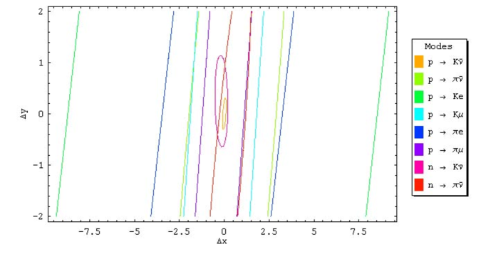
FIG. 3.: Allowed Region for $(x,y)$ coming from experimental lower limits on lifetimes for different decay modes for $z=0.329$. The point $(\Delta x,\Delta y)=(0,0)$ corresponds to $(x,y)=(-0.036,0.387)$. Note that the region is most constrained by $p\rightarrow K+\bar{\nu}$ mode.

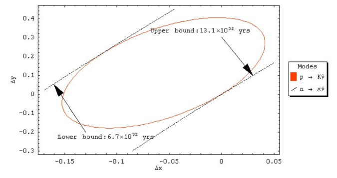
FIG. 4.: Upper limit on the $n\rightarrow\pi+\bar{\nu}$ partial lifetime while satisfying bounds on the lifetimes of all other modes. The point $(\Delta x,\Delta y)=(0,0)$ corresponds to $(x,y,z)=(-0.132,0.347,0.306)$.

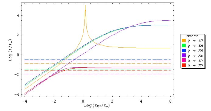
FIG. 5.: This figure gives the values of the lifetimes for different proton decay modes as a function of the lifetime of the $p\rightarrow K^{0}\mu^{+}$ mode (represented here by $log_{10}\frac{\tau_{K\mu}}{\tau_{0}}$ where $\tau_{0}=14.6\times 10^{33}$ years) when $\tau(p\rightarrow K^{+}\bar{\nu})$ mode is at its maximum value. This figure displays the values for one range of $(x,y,z)$ and the following figure does it for a complementary range. Also note that we have not included the gauge boson exchange diagrams, which provide a value for these lifetimes around $10^{36}$ years or so.

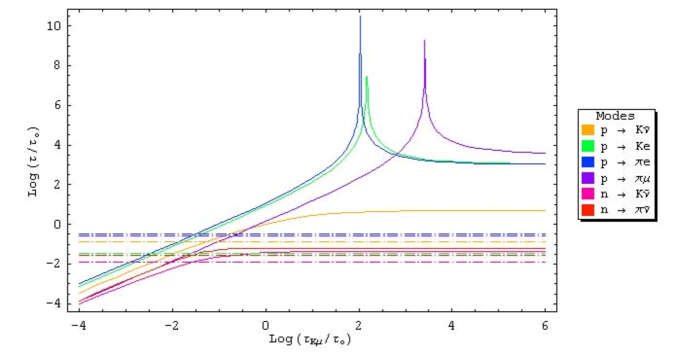
FIG. 6.: The same display as Fig. 5 but for a complementary range for the parameters $(x,y,z)$.

V Conclusion

In summary, we have discussed the predictions for nucleon decay in the minimal SO(10) model which has recently been shown to lead to predictions for neutrino masses and mixings in agreement with observations using only the assumption of type II seesaw mechanism. The key feature of this model is that B-L symmetry is broken by a single 126 field that also contributes to fermion masses. For the range of the parameters that are allowed by the neutrino data, we vary the GUT scale parameters ( unrelated to the neutrino sector) so as to satisfy the stringent experimental bounds for the decay mode $p\rightarrow K^{+}+\bar{\nu}$. We then predict an upper limit for the lifetimes for the modes $p\rightarrow\pi^{+}+\bar{\nu}$ and $n\rightarrow\pi^{0}\bar{\nu}$ as follows: $\tau(n\rightarrow\pi^{0}\bar{\nu})=2\tau(p\rightarrow\pi^{+}\bar{\nu})\leq 5.7-13\times 10^{32}$ years and $\tau(n\rightarrow K\bar{\nu})\leq 2.9\times 10^{33}$ yrs for the wino masses of 200 GeV and squark and slepton masses of a TeV. This should provide new motivations for a new search for proton decay, more specifically for these decay modes in question.

This work is supported by the National Science Foundation Grant No. PHY-0099544. We like to thank K. S. Babu, Tony Mann, J. C. Pati, J. Schechter, G. Senjanović and K. Turzynski for useful discussions and comments.

REFERENCES

- [1] J. C. Pati and A. Salam, Phys. Rev. D 10, 240 (1974); H. Georgi and S. L. Glashow, Phys. Rev. Lett. 32, 438 (1974).
- [2] S. Dimopoulos, S. Raby and F. Wilczek, Phys. Rev. D24, 1681 (1981); L. Ibanez and G. Ross, Phys. Lett. B 105, 439 (1981); M. Einhorn and D. R. T. Jones, Nucl. Phys. B 196, 475 (1982); W. Marciano and G. Senjanović, Phys. Rev. D25, 3092 (1982); U. Amaldi, W. de Boer and H. Furstenau, Phys. Lett. B260, 447 (1991); P. Langacker and M. Luo, Phys. Rev. D44, 817 (1991); J. Ellis, S. kelly and D. Nanopoulos, Phys. Lett. B260, 131 (1991).
- [3] S. Dimopoulos, S. Raby and F. Wilczek, Phys. Lett 112B, 133 (1982); J. Ellis, D. V. Nanopoulos and S. Rudaz, Nucl. Phys. B 202, 43 (1982).
- [4] M. Matsumoto, J. Arafune, H. Tanaka and K. Shiraishi, Phys. Rev. D46, 3966 (1992); J. Hisano, H. Murayama and T. Yanagida, Nucl. Phys. B402, 46 (1993).
- [5] P. Nath, R. Arnowitt and A. Chamseddine, Phys. Rev. D32, 2348 (1985); P. Nath and R. Arnowitt, Phys. Rev. D38, 1479 (1988).
- [6] H. Murayama and A. Pierce, Phys.Rev. D65, 055009 (2002).
- [7] B. Bajc, P. Perez and G. Senjanović, Phys.Rev. D66, 075005 (2002); hep-ph/0210374; D. Emmanuel-Costa and S. Wiesenfeldt, hep-ph/0302272
- [8] For discussion of proton decay in string theories, see T. Friedman and E. Witten, hep-th/0211269.
- [9] Super-Kamiokande collaboration, M. Shiozawa et al. Phys. Rev. Lett. 83, 1529 (1999).
- [10] For an extensive review, see A. Smirnov, hep-ph/0311259.
- [11] M. Gell-Mann, P. Ramond and R. Slansky, in Supergravity, eds. D. Freedman et al. (North-Holland, Amsterdam, 1980); T. Yanagida, in proc. KEK workshop, 1979 (unpublished); S. L. Glashow, Cargese lectures, (1979); R.N. Mohapatra and G. Senjanović, Phys. Rev. Lett. 44, 912 (1980).
- [12] For discussion of proton decay in models with 16 Higgs to break B-L, see V. Lucas and S. Raby, Phys. Rev. D55, 6986 (1997); K. S. Babu, J. C. Pati and F. Wilczek, Nucl. Phys. B 566, 33 (2000); K. Turzynski, hep-ph/0110282; JHEP 0210, 044 (2002); R. Dermisek, A. Mafi and S. Raby, Phys.Rev. D 63, 035001 (2001); I. Messina and C. Savoy, hep-ph/0309067; J. C. Pati, hep-ph/0305221.
- [13] K. S. Babu and R. N. Mohapatra, Phys. Rev. Lett. 70, 2845 (1993).
- [14] B. Bajc, G. Senjanović and F. Vissani, hep-ph/0210207; Phys. Rev. Lett. 90, 051802 (2003).
- [15] H. S. Goh, R. N. Mohapatra and S. P. Ng, hep-ph/0303055; Phys.Lett. B570, 215 (2003) and hep-ph/0308197; Phys. Rev. D, (to appear) (2003).
- [16] N. Sakai and T. Yanagida, Nucl. Phys. B 197, 533 (1982); S. Weinberg, Phys. Rev. D 26, 287 (1982).
- [17] C. S.Aulakh and R. N. Mohapatra, Phys. Rev. D 28, 217 (1983); N. Ohta, Prog. Theor. Phys. 70, 542 (1983); D. Chang, R. N. Mohapatra and M. K. Parida, Phys. Rev. D 30, 1052 (1984); J. Baseq, S. Meljanac and L. O’Raifeartaigh, Phys. Rev. D 39, 3110 (1989); D. G. Lee, Phys. Rev. D 49, 1417 (1994); C. S. Aulakh, A. Melfo, B. Bajc, G. Senjanović and F. Vissani, hep-ph/0306242.
- [18] D. G. Lee and R. N. Mohapatra, Phys. Rev. D 51, 1353 (1995); C. S. Aulakh, A. Melfo, A. Rasin, G. Senjanovic, Phys. Lett. B 459, 557 (1999); C. S. Aulakh, B. Bajc, A. Melfo, A. Rasin, G. Senjanovic, hep-ph/0004031.
- [19] R. N. Mohapatra and G. Senjanović, Phys. Rev. D 23, 165 (1981); C. Wetterich, Nuc. Phys. B 187, 343 (1981); G. Lazarides, Q. Shafi and C. Wetterich, Nucl.Phys.B181, 287 (1981).
- [20] J. Schechter and J. W. F. Valle, Phys. Rev. D22, 2227 (1980); E. Ma and U. Sarkar, Phys. Rev. Lett. 80, 5716 (1998).
- [21] SNO collaboration; Q. R. Ahmed et al. Nucl-ex/0309004.
- [22] P. Nath and R. Syed, hep-ph/0103165.
- [23] T. Goto and T. Nihei, hep-ph/9808255.
- [24] V. M. Belayev and M. Vysotsky, Phys. Lett. 127B, 215 (1983); K. S. Babu and S. M. Barr, hep-ph/9506261.
- [25] A. Masiero, in Perspectives on Supersymmetry, ed. G. Kane (World Scientific,1999).
- [26] M. Claudson, L. Hall and M. Wise, Nucl. Phys. B195, 297 (1982); S. Chadha and M. Daniel, Nucl. Phys. B229, 105 (1983); Y. Kuramashi et al. JLQCD collaboration, hep-ph/0103264; Phys. Rev. D 62, 014506 (2000).
- [27] K. Hirata et al. Phys. Lett. B220, 308 (1989).
- [28] D. Wall et al. Phys. Rev. D 62, 092003 (2000).
- [29] See R. E. Marshak, Riazuddin and C. P. Ryan, Theory of weak interactions, John Wiley (1969), p. 403.