The Flux Tube Model: Applications, Tests, and Extensions

Abstract

A review and critique of the Isgur-Paton flux tube model of hadronic physics is presented. This entails a detailed comparison with recent lattice gauge theory results which exposes both the successes and shortcomings of the model. Applications to hybrid masses, meson and hybrid meson decays, hadronic charge radii, the spin-orbit force, baryonic hybrids, and hybrid photocouplings are also discussed. Finally, I comment on the issue of adiabatic surface crossing which appears in both the flux tube model and lattice studies.

1 Flux Tubes

The impending upgrade of CEBAF at Jefferson Lab and the advent of a new experimental facility, Hall D, devoted in large part to the exploration of the gluonic excitations of QCD make it a propitious time to review the flux tube model. The flux tube model (FTM) of Isgur and Paton is now nearly 20 years oldIP and much has been learned in the meantime. This note shall review the foundations and predictions of the FTM and compare it, where possible, to lattice gauge or other theoretical tests. Extensions of the original ideas and new applications are also treated.

The flux tube model is an attempt to form a tractable model of low energy QCD which is based on longstanding ideas of string-like gluonic degrees of freedom. The central idea is that gluons should rearrange themselves into flux tubes which, in the heavy quark limit, adjust their configuration instantaneously in response to quark motion. Thus quarks are constrained to move on adiabatic gluonic energy surfaces. The lowest such surface is the familiar ‘Coulomb+linear’ potential of the constituent quark model and lattice gauge theory. States based on this surface thus form the ‘conventional’ mesons of the quark model. Higher adiabatic surfaces represent gluonic excitations and mesons built on these surfaces correspond to ‘hybrids’hyb . Thus the flux tube model is a simple and intuitive way to extend the nonrelativistic constituent quark model to include gluonic degrees of freedom.

The model was originally motivated through a series of truncations on the Euclidean time strong coupling QCD Hamiltonian with a lattice regulator (Hamiltonian lattice gauge theory). The degrees of freedom are quarks fields on lattice sites and gluonic ‘link variables’ $U_{\ell}=\exp(-iagA_{\mu}(x))$ where $\ell$ represents the link ($x,\hat{\mu}$). In the strong coupling limit the Hamiltonian is given by

$$H_{scQCD}={g^{2}\over 2a}\sum_{\ell}E_{\ell}^{a}E_{a\ell}+m\sum_{n}\bar{\psi}_{n}\psi_{n}$$ (1)

where $g$ is the strong coupling, $a$ is the lattice spacing, and $n$ is a lattice site. The velocity variables $\dot{U}_{\ell}$ have been replaced by electric field operators $E_{\ell}$. Gauge invariant pure glue states are formed by closed (possibly multiply connected) loops of link operators. The commutation relation $[E^{a},U]=T^{a}U$ then implies that the energy of these states is simply the sum of the quadratic colour charges of each link:

$$E_{\rm loop}={g^{2}\over 2a}\sum_{\ell\in{\rm loop}}{\cal C}_{\ell}^{2}$$ (2)

where ${\cal C}^{2}=4/3$ for a field in the 3 or $\bar{3}$ representations, 10/3 for 6 or $\bar{6}$, etc. The presence of quarks permits gauge invariant states with open flux strings which terminate on quark colour sources or sinks. Perturbations to these states are provided by subleading quark hopping and magnetic terms. The former allow flux tube breaking via quark pair production or quark motion. The latter can change link colour representations, cause link hopping, or change loop topology.

Isgur and Paton simplify the dynamics by (i) assuming an adiabatic separation of quark and gluon degrees of freedom (ii) neglecting ‘topological mixing’ such as loop breaking or loop Euler number changing transitions (iii) working in the nonrelativistic limit. The model is meant to be applied to the ‘intermediate regime’ where $1/a\sim\sqrt{b}$. They then model link variable dynamics in terms of spinless colourless particles (‘beads’) of mass $ba$ where $b$ is the string tension in the static quark potential. Finally these particles are assumed to interact via a linear potential and perform small oscillations about their resting positions. The result is a simple discrete string model for glue described by the Hamiltonian:

$$H=b_{0}R+\sum_{n}\left[{p_{n}^{2}\over 2b_{0}a}+{b_{0}\over 2a}(y_{n}-y_{n+1})^{2}\right],$$ (3)

where $y_{n}$ is the transverse displacement of the $n$th of $N$ string masses , $p_{n}$ is its momentum, $b_{0}$ is a bare string tension, and $R=(N+1)a$ is the separation between the static quarks. This Hamiltonian may be diagonalised in the usual way yielding

$$H_{FTM}=b_{0}R+\left({4\over\pi a^{2}}R-{1\over a}-{\pi\over 12R}+\ldots\right)+\sum_{n\lambda}\omega_{n}\alpha_{n\lambda}^{\dagger}\alpha_{n\lambda}$$ (4)

where $\alpha_{n\lambda}^{\dagger}$ creates a phonon in the $n$th mode with polarization $\lambda$. Notice that the string tension has been renormalized by the first term in brackets. The last term in brackets is the Lüscher term of string phenomenologyL . The mode energies are given by $\omega_{n}=2/a\sin[\pi n/2(N+1)]$. Thus $\omega_{1}\to\pi/R$ as $N\to\infty$ is the splitting between the ground state Coulomb+linear potential and the first gluonic excitation surface at long range. The energy of a given phonon state is approximately

$$E=E_{0}+N{\pi\over R}$$ (5)

with

$$N=\sum_{m=1}^{\infty}m(n_{m+}+n_{m-})$$ (6)

where $n_{m\pm}$ is the number of left (right) handed phonons in the $m$th mode.

2 Hybrids

Hybrid mesons are constructed by specifying the gluonic states via phonon operators and combining these with quark operators with a Wigner rotation matrix:

$$|LM_{L};s\bar{s};\Lambda,\{n_{m+},n_{m-}\}\rangle\propto\int d^{3}r\varphi(r)D^{L}_{M_{L}\Lambda}(\hat{r})\,b^{\dagger}_{r/2,s}d^{\dagger}_{-r/2,\bar{s}}\prod_{m}(\alpha_{m+}^{\dagger})^{n_{m+}}(\alpha_{m-}^{\dagger})^{n_{m-}}|0\rangle.$$ (7)

The projection of the total angular momentum on the $q\bar{q}$ axis is denoted by $\Lambda=\sum_{m}(n_{m+}-n_{m-})$. The parity and charge parity of these states are given by

$$P|LM_{L};SM_{S};\Lambda,\{n_{m+},n_{m-}\}\rangle=(-)^{L+\Lambda+1}|LM_{L};SM_{S};-\Lambda,\{n_{m-},n_{m+}\}\rangle,$$ (8)

$$C|LM_{L};SM_{S};\Lambda,\{n_{m+},n_{m-}\}\rangle=(-)^{L+S+\Lambda+N}|LM_{L};SM_{S};-\Lambda,\{n_{m-},n_{m+}\}\rangle.$$ (9)

States of good parity are thus formed as

$$|LM_{L};SM_{S};\zeta;\Lambda,\{n_{m+},n_{m-}\}\rangle={1\over\sqrt{2}}\Big{(}|LM_{L};SM_{S};\Lambda,\{n_{m+},n_{m-}\}\rangle+\zeta|LM_{L};SM_{S};-\Lambda,\{n_{m-},n_{m+}\}\rangle\Big{)}$$ (10)

Possible single phonon $(m=1)$ mesons are listed in Table I. Underlined quantum numbers represent quantum number exotic hybrids (mesons with quantum numbers not available to a $q\bar{q}$ state).

$\zeta$	$L$	$S$	$J^{PC}$
+	1	0	$1^{++}$
+	1	1	$(\underline{2},1,\underline{0})^{+-}$
+	2	0	$2^{--}$
+	2	1	$(\underline{3},2,\underline{1})^{-+}$
-	1	0	$1^{--}$
-	1	1	$(2,\underline{1},0)^{-+}$
-	2	0	$2^{++}$
-	2	1	$(3,\underline{2},1)^{+-}$

Table 1: Some Single Phonon Mesons.

Isgur and Paton obtained hybrid meson masses by solving a model Hamiltonian of quark motion on the single-phonon excited surface:

$$H_{IP}=-{1\over 2\mu}{\partial^{2}\over\partial r^{2}}+{L(L+1)-\Lambda^{2}\over 2\mu r^{2}}-{4\alpha_{s}\over 3r}+{\pi\over r}(1-{\rm e}^{-f\sqrt{b}r}).$$ (11)

The interaction term incorporates several important additional assumptions. Namely the $\pi/r$ phonon splitting is softened at short range. The parameter $f$ which appears in the softening function was estimated to be roughly unityIP . Furthermore, it was assumed that the attractive Coulomb ($1/r$) potential remains valid for hybrid mesons. Note that this is at odds with the expected

$$V_{oge}=+{\alpha_{s}\over 6r}$$ (12)

potential of perturbative one gluon exchange (the colour factor is that appropriate to gluon exchange between quarks in a colour octet state). This is an important assumption which will be examined in more detail below.

Finally the quark angular momentum operator is now complicated by the presence of gluonic/string degrees of freedom. One may write

$$L_{q\bar{q}}=L-L_{S_{||}}-L_{S_{\perp}}$$ (13)

where $L$ ($L_{S}$) is the total (string) angular momentum. Note that $L_{S_{\perp}}$ mixes adiabatic surfaces. Using $L_{S_{||}}=\Lambda\hat{r}$ and neglecting surface mixing yields the centrifugal term of Eq. 11. This additional assumption will also be examined in the next section.

The hybrid masses obtained by solving Eq. 11 are labelled $E_{IP}$ in Table II. Isgur and Paton also estimated the effects of adiabatic surface mixing and used these as their final mass estimates (labelled $E_{IP}^{\prime}$). The column labelled KW is explained in the next section. Finally, Table I implies that hybrids with quantum numbers $2^{\pm\mp}$,$1^{\pm\mp}$,$0^{\pm\mp}$,$1^{\pm\pm}$ are all degenerate at this order in the FTM.

flavour	$E_{IP}$	$E_{IP}^{\prime}$	$E_{KW}$KW
I=1	1.67	1.9	1.85
I=0	1.67	1.9	1.85
$s\bar{s}$	1.91	2.1	2.07
$c\bar{c}$	4.19	4.3	4.34
$b\bar{b}$	10.79	10.8	10.85

Table 2: Hybrid Mass Predictions

The next section will present a survey of possible tests of this ‘zeroth order’ Flux Tube Model.

3 Testing the Flux Tube Model

3.1 Small Oscillation and Adiabatic Approximations

The small oscillation approximation may be tested by considering a model of transverse beads interacting via a linear potential. Numerically solving such a HamiltonianBCS reveals that the small oscillation approximation is accurate for long strings but overestimates gluonic energies by an increasing amount as the interquark distance shrinks. Typical energy differences are order 100 MeV at 1 fm. Similarly, the adiabatic approximation can be tested by numerically solving the coupled quark-bead system. One findsBCS that the adiabatic approximation underestimates true energies by roughly 100 MeV, with slow improvement as the quarks get very massive. It thus appears that these approximation errors tend to cancel each other, leaving the IP predictions intact.

3.2 Gluonic Surfaces

Recent advances in computational speed and algorithms make it possible to test some of the assumptions of the FTM against the predictions of lattice gauge theory. Figure 1 shows the assumed ground state Coulomb+linear (solid line) and first excited state (dashed line) potentials of Isgur and Paton. These are compared to lattice Wilson loop computations of the same interactions (points)JKM . It is apparent that the IP potential overestimates the strength of the Coulomb potential and underestimates the string tension. Of course both of these model parameters are obtained by fitting the meson spectrum and therefore include effects which are not in the Wilson loop.

Figure 1: Comparison of the Potentials of Eq. 11 with lattice gauge theoryJKM .

3.2.1 Should the Coulomb Potential Appear?

More troubling is the first excited potential (bursts) which shows signs of saturating (or perhaps turning repulsive) at small distances, in disagreement with the assumption of Isgur and Paton. Indeed, simply omitting the attractive Coulomb portion of the IP hybrid potential dramatically improves agreement of the model with the lattice.

This disagreement represents something of a conundrum because Isgur and Paton had a good physical reason to employ the colour singlet $q\bar{q}$ Coulomb interaction in their model: if one assumes the repulsive short range interaction of Eq. 12, it becomes energetically favourable for the system to emit a gluon once the interquark separation becomes small enough. This gluon combines with the ‘valence’ gluon of the hybrid to form a scalar glueball, thereby changing the quark colour configuration to that of a singlet, and the Coulomb potential to the attractive form of Eq. 11. The point at which this should happen is indicated by the arrow in Fig. 2. It is clear that the lattice sees no such behaviour. This may be simply because the minimal relative momentum permitted on the lattices employed in the study were too coarse to permit the decay.

A physical reason for the suppression of this coupling is also possible. For example, if one considers the hybrid to be dominated by a Fock space component consisting of a constituent quark, antiquark, and gluon, then the postulated transition occurs through gluon emission from either the valence gluon or a valence quark. In the former case the coupling to a glueball is zero due to the colour overlap while in the latter case the coupling is suppressed by the large (infinite) quark mass. Thus one expects the coupling between the surfaces to be very small, which implies that the surface mixing will not be seen unless lattices with exceptionally large temporal extents are employed.

Which short distance behaviour should the model use? It seems clear that surface mixing which changes Fock sectors should not be used in a potential model. Rather, such mixing should be incorporated by explicitly including the appropriate transition operator in the formalism. Thus, for example, flux tube breaking is expected to eliminate the linear potential for distances beyond roughly one fermi when light quarks are present. However, such a truncated linear potential should not be used to construct mesons, rather one should employ the linear potential to form a basis of bound states and then include mixing to four quark states in an appropriate form. This approach avoids the unpleasant situation of having a mesonic ionization energy. Similarly, the hybrid potential should not include the mixing term since this mixes hybrid with hybrid+glueball Fock states.

Figure 2: Adiabatic Surface Crossing.

3.2.2 Higher Surfaces

The FTM predicts an entire tower of hybrid surfaces and it is interesting to examine their form in light of lattice data. Juge, Kuti, and Morningstar have carried out a detailed analysis of the relationship of the hybrid surfaces of Fig. 1 to the string excitations of Eq. 5JKMstring . They have found that surface excitations only have $\pi/r$ splittings for very large source separation (roughly 4 fermi or greater). This is shown in Fig. 3 where the dashed lines are the predicted $N\pi/r$ energy differences of the FTM. This is something of a surprise since one expects a phonon-like excitation spectrum on general grounds. It appears that QCD strings are complex objects at intermediate distance scales. Finally, the figure shows a cross over region at about 1 fermi where the surfaces move from a perturbative behaviour (characterized by the ‘gluelump’ spectrum) to a more string-like behaviour.

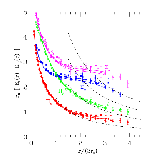
Figure 3: Hybrid Surface Energy Differences. 2$r_{0}$ is roughly 1 fermiJKMstring .

3.2.3 Hybrid Masses Revisited

In light of these issues it is appropriate to revisit the original hybrid mass estimates of Table I. A number of variants of the IP calculation were made in Ref. KW . Before presenting some of these, note that there is additional ambiguity in the quark angular momentum term of Eq. 11, namely it is also possible to set $L_{q\bar{q}}=L-J_{g}$ where $J_{g}$ is the total gluonic angular momentum. Squaring then yields

$$L_{q\bar{q}}^{2}=L(L+1)-2\Lambda^{2}+\langle J_{g}^{2}\rangle.$$ (14)

It has been found that setting $J_{g}$ = 2 yields good agreement with lattice dataJKMJg (this was also found in a constituent quark modelSS2 ). Notice that this is not numerically the same as the centrifugal term in Eq. 11.

Employing the hybrid lattice potential of Fig. 1 and Eq. 14 yields the hybrid masses labelled $E_{KW}$ in Table II. It is seen that these can differ by up to 200 MeV from the IP predictions of the second column. The similarity to the third column is a fluke since adiabatic surface mixing is not included in this computation. Merlin and Paton have noted that the majority of adiabatic mixing effects may be absorbed into the static potential by including the moment of inertia of the string in the centrifugal term (see the discussion below):

$${1\over 2\mu r^{2}}\to{1\over 2\mu r^{2}+{1\over 6}br^{3}},$$ (15)

and with a more important effect which modifies the strength of the $\pi/r$ splitting to be larger as $r$ becomes larger than $m_{q}/b$. Thus the final revisited prediction for a light hybrid is roughly 2.1 GeV.

4 The IKP Decay Model

Shortly after its introduction, the flux tube model of meson structure was extended by Isgur, Kokoski, and Paton to provide a description of mesonIK and hybridIKP decays. The transition operator was envisioned as arising due to the quark hopping term of the lattice QCD Hamiltonian. The lowest terms in the expansion of this operator are

$$H_{hop}=\sum_{n,\mu}\psi_{n}^{\dagger}\alpha\cdot\mu\psi_{n}+a\sum_{n,\mu}\psi_{n}^{\dagger}\alpha\cdot\mu\nabla\cdot\mu\psi_{n}.$$ (16)

If one assumes a smooth string then the first term dominates as the lattice spacing gets small and one has a ${}^{3}S_{1}$ strong decay operator. Alternatively, if the string is rough then the first term averages to zero upon summing over all local string orientations and the second term dominates, yielding a ${}^{3}P_{0}$ strong decay operator. The authors of Ref. IK ; IKP assume the second scenario since it is supported by experimentGS .

Flux tube degrees of freedom were incorporated by assuming factorization:

$$\langle\{\ldots\}bd;\{\ldots\}bd|{\cal O}|\{\ldots\}b^{\dagger}d^{\dagger}\rangle\approx\langle bd;bd|^{3}P_{0}|b^{\dagger}d^{\dagger}\rangle\cdot\langle\{\ldots\};\{\ldots\}|\{\ldots\}\rangle$$ (17)

The first matrix element on the right hand side is a typical ${}^{3}P_{0}$ mesonic decay overlap. The second represents the overlap of the gluonic/flux tube degrees of freedom. Assuming that the quark pair creation occurs at a transverse distance $y_{\perp}$ from the interquark axis of the parent meson yields the results

$$\langle\{0\ldots\};\{0\ldots\}|\{0\ldots\}\rangle\sim{\rm e}^{-fby_{\perp}^{2}}$$ (18)

for meson decay and

$$\langle\{0\ldots\};\{0\ldots\}|\{1\ldots\}\rangle\sim y_{\perp}{\rm e}^{-fby_{\perp}^{2}}$$ (19)

for hybrid decay. The factor $f$ is a computable constant of order unity. The extra factor of $y_{\perp}$ in the hybrid decay vertex forces the decay to pairs of identical $S$-wave mesons to be zero. This is the origin of the famous ‘S+D’ selection rule in this model (it occurs in other models for different reasons).

Unfortunately, it will be some time before lattice gauge theory has progressed to the point where models such as these can be thoroughly tested. However, preliminary computations reveal that a substantial closed flavour decay mode (such as $b\bar{b}g\to\chi_{b}\eta$) may existUKQCD . In the meantime we hope that experiment will provide some clues. An alternative decay model is discussed in the next section.

5 Extensions

The hadronic decay model of the proceeding section is its most well known extension. However, the model has been extended in several other directions as well; some of these are described here.

5.1 Charge Radii and Hybrid Decays

Several years ago Isgur pointed out that the energy carried by the flux tube will change several features of the naive quark modelI (see also MP2 ). For example, zero point oscillation of the flux tube about the interquark axis will induce transverse fluctuations in the quark positions, something which is not present when the flux tube is treated as potential. The additional fluctuations have the effect of increasing the charge radius of a heavy-light meson (qQ):

$$r_{Q}^{2}=\left[\left({m_{q}\over m_{q}+m_{Q}}\right)^{2}+{2b\over\pi^{3}m_{q}^{2}}\zeta(3)\right]\langle r^{2}\rangle$$ (20)

where the second term in the bracket is the new contribution. He estimated this to give rise to a 50% increase in charge radii of light quark hadrons.

This observation has subsequently been expanded upon by Close and Dudek who observe that radiative decays of hybrid mesons may proceed because the recoil of the radiating quark affects the string degrees of freedom giving a nonzero overlap of the flux tube wavefunction with the ground state flux tube wavefunctions of ordinary mesons. Preliminary computations with this mechanism have appearedCD .

A similar scheme involving the emission of pointlike pions may be used to compute hybrid decays to final states such as $\pi\rho$CD2 . The most striking result here is that this decay mechanism evades the ‘S+D’ suppression discussed above.

5.2 Adiabatic Surface Mixing

Merlin and Paton examined the effects of adiabatic surface mixing on the leading order FTM by considering the complete quark-bead system ab initioMP . Although the effects can be quite complicated, with mixing to all surfaces possible, they found that the majority of the effects can be absorbed in a redefinition of the hybrid potential by including the rigid body moment of inertia of the string in the centrifugal term and by modifying the strength of the $\pi/r$ term (see Eq. 15).

An explicit computation revealed found mass shifts of order -100 MeV for conventional S-wave light quark mesons and +200 MeV for light quark hybrids. The resulting mass splittings are quoted in column three of Table I and were used by Isgur and Paton to form their final estimates of the lowest lying hybrid masses.

5.3 Spin Orbit Forces I

Merlin and Paton also examined spin orbit forces in the context of the FTMMP2 . The idea was to map the operators of the leading spin orbit term in the heavy quark expansion of QCD, namely $V_{SO}=g/2m\,{\bm{\sigma}}\cdot{\bf B}$, onto FTM degrees of freedom (phonons). Merlin and Paton did this by identifying the magnetic field with the lattice operator

$$T^{a}B^{a}(x)\sim{1\over 2ga^{2}}\left(U_{P}(x)-U_{P}^{\dagger}(x)\right).$$ (21)

Since the plaquette operator moves flux links in a fixed topological sector, it is natural to identify the magnetic field with the bead kinetic energy. Doing so then allows one to write $V_{SO}$ in terms of phonons.

Explicit computations revealed that spin orbit splittings due to $V_{SO}$ are small and that the majority of the splittings arise from Thomas precession, $V_{Th}={1\over 4}(\ddot{\bm{r}}_{q}\times\dot{\bm{r}}_{q})\cdot{\bm{\sigma}}$. This is modelled by including the effects of phonons on the quark coordinate (see the discussion of the charge radii above). The mass splittings for light hybrids are listed in Table III. One sees that the lowest member of the octet of light hybrids is predicted to be the $2^{+-}$ while the heaviest is the $0^{+-}$. This appears to be in conflict with lattice gauge theory which finds that the lightest hybrids are $1^{-+}$.

$J^{PC}$	$2^{+-}$	$2^{-+}$	$1^{-+}$	$0^{-+}$	$1^{+-}$	$0^{+-}$	$1^{++}$	$1^{--}$
$\delta M$ (MeV)	-140	-20	20	40	140	280	0	0

Table 3: Spin Orbit Hybrid Mass SplittingsMP2 .

5.4 Spin Orbit Forces II

Spin-dependent forces in the FTM were also taken up by the authors of Ref. SS4 in an attempt to resolve a conundrum in the spin-orbit sector of the quark interaction. The issue is that many models of hadrons prefer a vector Dirac structure of confinement, rather than the phenomenologically accepted Dirac scalar interaction. This may be studied by using the heavy quark Foldy-Wouthyusen version of the QCD Hamiltonian in Coulomb gauge. The resulting ${\cal O}(1/m)$ and ${\cal O}(1/m^{2})$ operators, $H_{1}$ and $H_{2}$, depend on the chromoelectric and magnetic fields and hence are nonperturbative. In a similar approach to that of Merlin and Paton, the authors of Ref. SS4 chose to study these operators by mapping the chromofields to phonons. In this case the mapping was based on the idea that the electric field counts string length and therefore should be mapped as $E_{\lambda}^{a}(x=na)={\sqrt{b_{0}}\over a^{2}}\left(y^{a}_{\lambda}(n+1)-y^{a}_{\lambda}(n)\right)$ where $a$ is a colour index and $\lambda$ is a polarization index. Imposing the canonical commutation relations gives the magnetic field as a derivative with respect to transverse displacement. Finally both expressions can be mapped to phonon degrees of freedom with the standard Fourier transform. Notice that this approach has the flux tube beads carrying colour charge.

The form of the effective spin-dependent interactions were then evaluated by inserting these field operators into $H_{1}$ and $H_{2}$. It was found that an effective scalar spin orbit interaction could indeed arise in the flux tube picture of hadronic structure even though the static confining interaction was vector. This was the case because nonperturbative mixing of mesons with hybrids contribute to spin-dependent interactions and can change the naive expectations based on the nonrelativistic reduction of a simple interaction kernel.

5.5 Vector Decay Model

The same chromofield–phonon mapping which was used in the study of the spin orbit interactionSS4 was used to examine hybrid decays in Refs. PSS . In this case the operator of interest is simply $V=-g\int\bar{\psi}{\bm{\alpha}}\cdot{\bf A}\psi$. The resulting decay vertex is given by

$$H_{int}={iga^{2}\over\sqrt{\pi}}\sum_{m,\lambda}\int_{0}^{1}d\xi\cos(\pi\xi)T^{a}_{ij}\,b^{\dagger}_{i}(\xi{\bf r}_{Q\bar{Q}}){\bm{\sigma}}\cdot\hat{\bf e}_{\lambda}(\hat{\bf r}_{Q\bar{Q}})\left(\alpha^{a}_{m\lambda}-\alpha^{a\dagger}_{m\lambda}\right)d^{\dagger}_{j}(\xi{\bf r}_{Q\bar{Q}}),$$ (22)

where the $\hat{\bf e}(\hat{\bf r})$ are polarization vectors orthogonal to $\hat{\bf r}$. The integral is defined along the $Q\bar{Q}$ axis only. This model also has an ‘S+D’ decay rule, however in contrast to the IKP decay model this is due to a node along the interquark axis (the $\cos(\pi\xi)$) which causes the selection rule, rather than a node perpendicular to the interquark axis.

The phenomenology of this model has been presented in the second of Ref. PSS . One finds that it is similar to a ${}^{3}S_{1}$ model of meson decays in that $D$ wave decay modes tend to be suppressed. Recent comparison with experiment have proven surprisingly accurate and lend support to hybrid interpretations for nonexotic $2^{-+}(2003)$ and $1^{++}(2096)$ statesJK .

5.6 Hybrid Baryons

Capstick and Page have made a detailed study of baryon flux tube dynamicsCP . This is a technically challenging problem due to the multitude of vibrational and rotational modes which are available to a Y-shaped string system. However, they have found that the problem simplifies considerably because the string junction decouples to good accuracy from the rest of the bead motion. Thus a hybrid baryon can be approximated by three quarks coupled via linear potentials to a massive ‘junction bead’. The dynamics of this system are completely specified by the FTM and variational calculations indicate that the lowest lying hybrids are $J^{P}={1\over 2}^{+}$ and ${3\over 2}^{+}$ states at approximately 1870 MeV.

Happily, lattice investigations of the static baryon interaction have begunBFT . The chief point of interest is whether the expected flux tubes form into a ‘Y’ shape or a ‘$\Delta$’ shape. This may be addressed by carefully examining the baryonic energy in a variety of quark configurations. Current results are mixed, with some groups claiming support for the two-body hypothesis Alexandrou and some for the three-body hypothesisSuganuma . Finally, a strong operator dependence in the flux tube profiles has been observedOW , which clearly needs to be settled before definitive conclusions can be reached.

6 Conclusions

The flux tube model is now nearly 20 years old. In this time it has been applied to an increasing array of problems and extended in several directions, chiefly by taking seriously the idea that dynamical string-like gluonic degrees of freedom are important in the low lying mesons. A number of additional extensions are:

(i) glueballs (glue loops). A preliminary study has been made in the original paperIP , however much remains to be done here. Comparison with lattice gauge theory will provide a crucial test.

(ii) FT effects in baryons. The charge radii ideas of Isgur, Close, and Dudek have immediate impact on baryons and should be studied.

(iii) adiabatic surfaces. It is worthwhile to attempt to leverage new precise lattice data on the gluelump spectrum and the hybrid adiabatic surfaces to improve the FTM in detail.

(iv) the FTM may allow one to improve the semiclassical fragmentation formalismIP .

(v) long range spin-spin and spin-orbit forces should be re-examined in an attempt to pin down this difficult aspect of nonperturbative QCD.

In summary, the FTM provides a compelling picture of strong QCD dynamics; however, it is a picture only! We have seen that the FTM correctly describes the level orderings and, perhaps, splittings of gluonic adiabatic energy surfaces at large distances (perhaps as large as 4 fm). The model fails to describe the spectrum at small interquark distances (although, of course, it can be amended). Furthermore, the original IP model of hybrids is likely to be incorrect in many details, although its phenomenology may be surprisingly robust. We have seen that it is possible to extend the model in many different ways. Of course these extensions rely on detailed aspects of the FTM which are untested at best. It appears likely, for example, that the spin orbit splitting of Ref. MP2 do not agree with lattice data. In the end, the utility of a tractable and appealing model should not be underestimated.

References

- (1) N. Isgur and J. Paton, Phys. Rev. D31, 2910 (1985).
- (2) R. Giles and S. H. Tye, Phys. Rev. Lett. 37, 1175 (1976); T. Barnes, Caltech Ph.D. thesis (1977); D. Horn and J. Mandula, Phys. Rev. D17, 898 (1978).
- (3) See for example, M. Luscher and P. Weisz, JHEP 0207, 049 (2002).
- (4) K. Waidelich, NCSU MSc thesis (2000).
- (5) T. Barnes, F. E. Close, and E. S. Swanson, Phys. Rev. D 52, 5242 (1995).
- (6) K.J. Juge, J. Kuti, and C.J. Morningstar, Nucl. Phys. Proc. Suppl. 63, 326 (1998).
- (7) C. J. Morningstar, K. J. Juge and J. Kuti, Nucl. Phys. Proc. Suppl. 73, 590 (1999); K. J. Juge, J. Kuti and C. Morningstar, Phys. Rev. Lett. 90, 161601 (2003).
- (8) R. Kokoski and N. Isgur, Phys. Rev. D35, 907 (1987).
- (9) N. Isgur, R. Kokoski, and J. Paton, Phys. Rev. Lett. 54, 869 (1985).
- (10) P. Geiger and E. S. Swanson, Phys. Rev. D 50, 6855 (1994).
- (11) C. McNeile, C. Michael, and P. Pennanen [UKQCD Collaboration], Phys. Rev. D 65, 094505 (2002).
- (12) N. Isgur, Phys. Rev. D60, 114016 (1999).
- (13) F. E. Close and J. J. Dudek, Phys. Rev. Lett. 91, 142001 (2003); F. E. Close and J. J. Dudek, “Hybrid meson production by electromagnetic and weak interactions in a flux-tube simulation of lattice QCD”, arXiv:hep-ph/0308098.
- (14) F. E. Close and J. J. Dudek, “The ’forbidden’ decays of hybrid mesons to pi rho can be large”, arXiv:hep-ph/0308099.
- (15) J. Merlin and J. Paton, J. Phys. G11, 439 (1985).
- (16) J. Merlin and J. Paton, Phys. Rev. D35, 1668 (1987).
- (17) A.P. Szczepaniak and E.S. Swanson, Phys. Rev. D55, 3987 (1997).
- (18) A.P. Szczepaniak and E.S. Swanson, Phys. Rev. D56, 5692 (1997); P.R. Page, E.S. Swanson, A.P. Szczepaniak, Phys. Rev. D59, 014035 (1999).
- (19) Joachim Kuhn, “Evidence for Hybrid Mesons”, talk presented at Hadron 2003, Aschanffenburg, Germany (2003).
- (20) K.J. Juge, J. Kuti, and C.J. Morningstar, hep-lat/9709132.
- (21) E.S. Swanson and A.P. Szczepaniak, Phys. Rev. D59, 014035 (1999).
- (22) S. Capstick and P. R. Page, Phys. Rev. C 66, 065204 (2002).
- (23) H. Ichie, V. Bornyakov, T. Streuer and G. Schierholz, “The flux distribution of the three quark system in SU(3)”, arXiv:hep-lat/0212024.
- (24) C. Alexandrou, P. De Forcrand and A. Tsapalis, Phys. Rev. D 65, 054503 (2002).
- (25) T. T. Takahashi, H. Suganuma, Y. Nemoto and H. Matsufuru, Phys. Rev. D 65, 114509 (2002).
- (26) F. Okiharu and R. M. Woloshyn, “A study of colour field distributions in the baryon”, arXiv:hep-lat/0310007.