Abstract

We show how Lorentz invariance violation (LIV) can occur for Majorana neutrinos, without inducing LIV in the charged leptons via radiative corrections. Such “electrophobic” LIV is due to the Majorana nature of the LIV operator together with electric charge conservation. Being free from the strong constraints coming from the charged lepton sector, electrophobic LIV can in principle be as large as current neutrino experiments permit. On the other hand electrophobic LIV could be naturally small if it originates from LIV in some singlet “right-handed neutrino” sector, and is felt in the physical left-handed neutrinos via a see-saw mechanism. We develop the formalism appropriate to electrophobic LIV for Majorana neutrinos, and discuss experimental constraints at current and future neutrino experiments.

1 Introduction

Lorentz and CPT invariance are considered to be amongst the most sacred symmetries of elementary particle physics. However, this very reason should motivate us to search for the smallest of hints of their possible violation. Indeed, motivated in part by string theory, there has been some recent interest in the possibility that CPT and Lorentz invariance might be violated in nature [1, 2]. CPT violation (CPTV) and Lorentz invariance violation (LIV) [1, 2], are clearly interesting effects but subject to strong constraints coming from charged fermions. However in the neutrino sector, the limits are much weaker, and so one might hope to observe such non-standard effects in accurate neutrino oscillation experiments [3] due to CPTV terms of the form $\bar{\nu}_{L}^{\alpha}b^{\mu}_{\alpha\beta}\gamma^{\mu}\nu_{L}^{\beta}$, where $\nu_{L}$ represents left-handed neutrinos labelled by $\alpha,\beta$ and $b^{\mu}_{\alpha\beta}$ are CPTV constants. This operator leads to modifications of the neutrino oscillation formula as discussed in Appendix A. A detailed discussion on Lorentz and CPT violation in the neutrino sector has recently appeared in [4], where the most general Lagrangian for the neutrinos in the minimal Standard Model extension is presented, including a catalogue of all CPTV and LIV terms [4].

Although of great potential interest from the point of view of future neutrino experiments, to stand a chance of the effects being observable, any CPTV and LIV in the neutrino sector must be effectively screened from the charged lepton sector, since the strong limits arising from charged leptons would already preclude any observation in neutrino oscillation experiments. Two main requirements of any effective theory of Lorentz and CPT violation in the neutrino sector are therefore: (i) to explain the smallness of Lorentz and CPT violation; (ii) to protect the Lorentz and CPT violation in the neutrino sector from the bounds coming from the charged lepton sector [4].

An elegant way of satisfying (i) is to suppose that such effects originate in the “right-handed neutrino” singlet sector, and are only fed down to the left-handed neutrino sector via the see-saw mechanism, thereby giving naturally small LIV in the left-handed neutrino sector. This possibility is theoretically attractive since the “right-handed neutrinos” could represent any singlet sector, and need not be associated with ordinary quarks and leptons, except via their Yukawa couplings to left-handed neutrinos. The fact that CPT violation is associated only with such a singlet sector could provide a natural explanation for why CPT appears to be a good symmetry for charged fermions, while being potentially badly broken in the neutrino sector.

Although it is possible to satisfy (i) by appeal to the see-saw mechanism, in some cases it is not possible to satisfy (ii) at the same time. An example of a problematic case was discussed in [5] for the CPT violating operator $\bar{N}_{R}^{\alpha}B^{\prime\mu}_{\alpha\beta}\gamma^{\mu}N_{R}^{\beta}$ for the singlet right-handed neutrinos $N_{R}$ labelled by $\alpha,\beta$ and the $B^{\prime}$ are CPTV constants in the “right-handed neutrino” sector. The standard see-saw mechanism leads to naturally suppressed CPT violation in the left-handed neutrino sector of the type mentioned above, namely $\bar{\nu}_{L}^{\alpha}b^{\mu}_{\alpha\beta}\gamma^{\mu}\nu_{L}^{\beta}$, where now $b^{\mu}=m_{LR}^{2}B^{\prime\mu}/({B^{\prime}}^{2}+M_{RR}^{2})$ where $m_{LR}$ is the Dirac neutrino mass, and $M_{RR}$ is the heavy Majorana mass of the “right-handed neutrinos”. However the problem is [5] that the see-saw mechanism also generates unacceptably large CPT violation in the charged lepton sector via one-loop radiative corrections which yield the operator $\bar{L}_{L}^{\alpha}{b_{loop}}^{\mu}_{\alpha\beta}\gamma^{\mu}L_{L}^{\beta}$, where $L_{L}=(\nu_{L}~{}e_{L})^{T}$ is the $SU(2)_{L}$ doublet that contains the left-handed charged leptons and neutrinos, where $b_{electron}\sim b_{loop}^{\mu}\sim 10^{-2}b^{\mu}$ [5]. Since the limit from the electron is $b_{electron}<10^{-19}$ eV, this implies that in the neutrino sector $b<10^{-17}$ eV which renders any CPT violation in the neutrino sector unobservable.

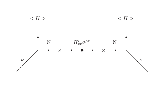
Figure 1: Tree level diagram giving rise to electrophobic see-saw suppressed LIV in the light physical left-handed neutrino $\nu$ sector due to a lepton number violating LIV operator in the right-handed neutrino $N$ sector. The dashed lines represent (possibly supersymmetric) standard model Higgs with vacuum expectation values $<H>$. The central blob represents insertion of the LIV operator in the right-handed neutrino sector, and the crosses indicate heavy right-handed Majorana masses.

In this paper we show how it is possible to satisfy both (i) and (ii) at the same time in a specific example in which the feed-down into the charged lepton sector is explicitly prevented by electric charge conservation. In this case it is possible to have naturally small (but still observable) LIV in the Majorana neutrino sector via the see-saw mechanism, without leading to any LIV in the charged lepton sector via radiative corrections, to all orders in perturbation theory. In order to ensure protection from bounds coming from the charged lepton sector the operators should be Majorana and lepton number violating. The essential point is that such operators, being lepton number violating, cannot lead to effects in the charged lepton sector due to electric charge conservation. As a consequence LIV could be large enough to be observable in the future neutrino experiments. We refer to such operators as electrophobic. We propose that such electrophobic operators arise exclusively from some heavy “right-handed neutrino” singlet sector, are fed down to physical light left-handed neutrinos via the see-saw mechanism shown in Fig. 1. The main purpose of this paper is to develop the formalism required for phenomenological studies of such electrophobic LIV operators, and to briefly study the experimental constraints at current and planned neutrino experiments.

The remainder of the paper is organised as follows. In section 2 and Appendix B we argue that only one electrophobic operator exists and show how it can give naturally small effects in the left-handed neutrino sector due to the see-saw mechanism, without inducing any charged lepton contributions. We also derive the equation of motion for the two flavour case. In section 3 we derive the neutrino oscillation probabilities in the presence of electrophobic LIV, and in section 4 we discuss the experimental constraints of electrophobic LIV at different experiments. Section 5 concludes the paper. Appendix A contains a derivation of the equation of motion and the neutrino survival probability for the usual CPT violating operator, $\bar{\nu}_{L}^{\alpha}b^{\mu}_{\alpha\beta}\gamma^{\mu}\nu_{L}^{\beta}$, while Appendix B is dedicated to the details of the electrophobic LIV Lagrangian in a two-generation formalism.

2 Operators, see-saw mechanism and equation of motion

In this section we shall first write down LIV operators in some “right-handed neutrino” singlet $N$ sector, arising from some high scale physics, possibly associated with the scale of heavy Majorana masses $M$. In principle $M$ may be associated with some string scale at which LIV may be manifest [1], but none of our results depend on this assumption. In order to be electrophobic the operator should be Majorana in nature, and violate lepton number by $\Delta L=2$. Therefore we are interested in operators like $(\overline{N_{R}^{C}})_{\alpha}{\cal O}_{\alpha\beta}(N_{R})_{\beta}$, where $N_{R}$ are right-handed neutrinos, $C$ represents charge conjugation, and $\cal{O}$ represents the remainder of the operator. There are only three such non-vanishing Majorana type fermion bilinears which break LIV:

$${H^{\prime}}_{\alpha\beta}^{\mu\nu}(\overline{N_{R}^{C}})_{\alpha}\sigma_{\mu\nu}(N_{R})_{\beta}$$ (1)

$${g^{\prime}}_{\alpha\beta}^{\mu}(\overline{N_{R}^{C}})_{\alpha}\partial^{\nu}\sigma_{\mu\nu}(N_{R})_{\beta};~{}{\rm and}~{}{g^{\prime\prime}}_{\alpha\beta}^{\lambda\mu\nu}(\overline{N_{R}^{C}})_{\alpha}\partial^{\nu}\sigma_{\lambda\mu}(N_{R})_{\beta}$$ (2)

where $\mu,\nu$ denote the Lorentz indices, $\alpha,\beta$ are flavor indices and $H^{\prime},g^{\prime},g^{\prime\prime}$ are LIV constants in the heavy “right-handed neutrino” sector. However, since the Majorana singlet that we are concerned with are very heavy, the terms in Eq.2 can be dropped in the static limit and the only remaining Majorana type LIV term which is relevant is that in Eq.1. The see-saw mechanism in Fig. 1 then induces LIV in the left-handed neutrino sector:

$${\cal L}_{LIV}\sim h_{\alpha\beta}^{\mu\nu}(\overline{\nu_{L}^{C}})_{\alpha}\sigma_{\mu\nu}(\nu_{L})_{\beta}$$ (3)

where $h^{\mu\nu}=m_{LR}^{2}{H^{\prime}}^{\mu\nu}/({H^{\prime}}^{2}+M_{RR}^{2})$. As already noted, because of the Majorana nature of the operator, LIV cannot be fed down to the charged lepton sector at any loop order, due to electric charge conservation. By comparison the usual CPT violating operator discussed in Appendix A is not Majorana, and so the charged lepton sector is not protected [5].

In Appendix B we expand ${\cal L}_{LIV}$ in a scenario with two neutrino flavors, $\nu_{\alpha}$ and $\nu_{\beta}$:

$${\cal L}_{LIV}=\bigg{[}(\nu^{C}_{\alpha R})^{\dagger}\nu_{\beta L}H_{+}-(\nu_{\alpha L})^{\dagger}\nu_{\beta R}^{C}H_{-}+(\nu_{\beta L})^{\dagger}\nu_{\alpha R}^{C}H_{-}-(\nu_{\beta R}^{C})^{\dagger}\nu_{\alpha L}H_{+}\bigg{]}$$ (4)

Therefore, in presence of the LIV operator that we consider, it is possible for a neutrino of a flavor $\alpha$ to transform into an antineutrino of another flavor $\beta$, as the neutrino beam propagates. This would give rise to neutrino-antineutrino oscillations between different flavors due to LIV. However, transitions between neutrino and antineutrino of the same flavor is strictly forbidden, since CPT is conserved.

The equation of motion for the two neutrino flavour case, including both the mass terms and the LIV terms, then follows as,

$$i\frac{d}{dt}\pmatrix{\nu_{\alpha L}\cr\bar{\nu}_{\alpha R}\cr\nu_{\beta L}\cr\bar{\nu}_{\beta R}\cr}=\pmatrix{-\delta\cos 2\theta&0&\delta\sin 2\theta&H_{-}\cr 0&-\delta\cos 2\theta&-H_{+}&\delta\sin 2\theta\cr\delta\sin 2\theta&-H_{-}&\delta\cos 2\theta&0\cr H_{+}&\delta\sin 2\theta&0&\delta\cos 2\theta\cr}\pmatrix{\nu_{\alpha L}\cr\bar{\nu}_{\alpha R}\cr\nu_{\beta L}\cr\bar{\nu}_{\beta R}\cr}$$ (5)

where $\delta=\Delta m^{2}/4E$, $\Delta m^{2}=m_{2}^{2}-m_{1}^{2}$ is the mass squared difference of the neutrinos and $E$ is the energy of the neutrino beam. The equation of motion for Majorana neutrinos with non-zero transition magnetic moment in the presence of a magnetic field also has a similar form [7].

3 Neutrino oscillation probabilities

In this section we look for the neutrino transition and survival probabilities in the presence of electrophobic LIV interactions. The neutrino mass matrix in the flavor basis can be written in vacuum as

$$M_{F}=\pmatrix{-\delta\cos 2\theta&0&\delta\sin 2\theta&H\cr 0&-\delta\cos 2\theta&-H&\delta\sin 2\theta\cr\delta\sin 2\theta&-H&\delta\cos 2\theta&0\cr H&\delta\sin 2\theta&0&\delta\cos 2\theta\cr}$$ (6)

where $H$ is the extra element due to LIV interaction. In the above we have expressed $H_{\pm}=He^{\pm i\phi}$ and have assumed $\phi=0$. We will show later that $\phi$ is related to the change in the neutrino oscillation probabilities with the direction of the propagation of the neutrino and is therefore an important parameter [4]. However for the sake of simplicity and to get an approximate idea about the constraint on the electrophobic LIV term from current and planned experiments, we choose to put $\phi=0$ in this and the next section. The case $\phi\neq 0$ will be considered in section 5. The mass matrix in Eq. 6 can be diagonalised and the eigenvalues are

$$\lambda_{1}=-\sqrt{\delta^{2}+H^{2}};~{}~{}\lambda_{2}=-\sqrt{\delta^{2}+H^{2}};~{}~{}\lambda_{3}=\sqrt{\delta^{2}+H^{2}};~{}~{}\lambda_{4}=\sqrt{\delta^{2}+H^{2}}$$ (7)

The corresponding mixing matrix $\tilde{U}$ in the presence of the LIV term is defined as

$$M_{F}=\tilde{U}^{\dagger}diag(\lambda_{1},\lambda_{2},\lambda_{3},\lambda_{4})\tilde{U}$$ (8)

and is given by

$$\tilde{U}=\frac{1}{\sqrt{2}}\pmatrix{\delta\sin 2\theta/D_{-}&H/D_{-}&\delta\sin 2\theta/D_{+}&H/D_{+}\cr-H/D_{-}&\delta\sin 2\theta/D_{-}&-H/D_{+}&\delta\sin 2\theta/D_{+}\cr-D_{-}/\sqrt{\delta^{2}+H^{2}}&0&D_{+}/\sqrt{\delta^{2}+H^{2}}&0\cr 0&-D_{-}/\sqrt{\delta^{2}+H^{2}}&0&D_{+}/\sqrt{\delta^{2}+H^{2}}}$$ (9)

where

$$D_{\pm}=\sqrt{\delta^{2}+H^{2}}\bigg{(}1\pm\frac{\delta\cos 2\theta}{\sqrt{\delta^{2}+H^{2}}}\bigg{)}^{1/2}$$ (10)

One can check that when $H=0$, the mixing matrix $\tilde{U}$ reduces to the vacuum mixing matrix in the standard case and there is no mixing between the neutrino and antineutrino states.

The general transition probability of a given flavor $\nu_{\alpha}$ to a flavor $\nu_{\beta}$ is given by

$$P_{\alpha\beta}=\delta_{\alpha\beta}-4\sum_{j>i}Re(\tilde{U}_{\alpha i}\tilde{U}_{\beta i}^{*}\tilde{U}_{\alpha j}^{*}\tilde{U}_{\beta j})\sin^{2}\bigg{(}\frac{\Delta\lambda_{ij}L}{2}\bigg{)}+2\sum_{j>i}Im(\tilde{U}_{\alpha i}\tilde{U}_{\beta i}^{*}\tilde{U}_{\alpha j}^{*}\tilde{U}_{\beta j})\sin\bigg{(}\Delta\lambda_{ij}L\bigg{)}$$ (11)

where $L$ is the distance traveled and $\Delta\lambda_{ij}=\lambda_{i}-\lambda_{j}$. We will assume that the mixing matrix $\tilde{U}$ is real so that the last term in Eq.(11) vanishes. Next we note that $\Delta\lambda_{12}=\Delta\lambda_{34}=0$ and $\Delta\lambda_{13}=\Delta\lambda_{14}=\Delta\lambda_{23}=\Delta\lambda_{24}=2\sqrt{\delta^{2}+H^{2}}$. Thus the expression for the probability in the two-generation limit that we consider here reduces to

$$P_{\alpha\beta}=\delta_{\alpha\beta}-4\bigg{[}\tilde{U}_{\alpha 1}\tilde{U}_{\beta 1}+\tilde{U}_{\alpha 2}\tilde{U}_{\beta 2}\bigg{]}\bigg{[}\delta_{\alpha\beta}-(\tilde{U}_{\alpha 1}\tilde{U}_{\beta 1}+\tilde{U}_{\alpha 2}\tilde{U}_{\beta 2})\bigg{]}\sin^{2}\bigg{(}\frac{\sqrt{(\Delta m^{2})^{2}+(4HE)^{2}}~{}L}{4E}\bigg{)}$$ (12)

We can now use Eq.(9) and (12) to get

$$P_{\alpha\alpha} = P_{\bar{\alpha}\bar{\alpha}}$$ (13)

$$= 1-\frac{(4HE)^{2}+(\Delta m^{2})^{2}\sin^{2}2\theta}{(4HE)^{2}+(\Delta m^{2})^{2}}\sin^{2}\bigg{(}\frac{\sqrt{(\Delta m^{2})^{2}+(4HE)^{2}}~{}L}{4E}\bigg{)}$$

$$P_{\alpha\beta} = \frac{(\Delta m^{2})^{2}\sin^{2}2\theta}{(4HE)^{2}+(\Delta m^{2})^{2}}\sin^{2}\bigg{(}\frac{\sqrt{(\Delta m^{2})^{2}+(4HE)^{2}}~{}L}{4E}\bigg{)}$$ (14)

$$P_{\alpha\bar{\beta}} = \frac{(4HE)^{2}}{(4HE)^{2}+(\Delta m^{2})^{2}}\sin^{2}\bigg{(}\frac{\sqrt{(\Delta m^{2})^{2}+(4HE)^{2}}~{}L}{4E}\bigg{)}$$ (15)

while $P_{\alpha\bar{\alpha}}=0$ identically, since CPT is conserved. It is again trivial to see that for $H<<\Delta m^{2}$ or $H=0$, the expressions for the probability reduces to the vacuum oscillation probabilities. On the other hand if $H\gg\mbox{$\Delta{m}^{2}$~{}}$ then,

$$P_{\alpha\alpha}=1-\sin^{2}\bigg{(}H~{}L\bigg{)}$$ (16)

$$P_{\alpha\beta}=0$$ (17)

$$P_{\alpha\bar{\beta}}=\sin^{2}\bigg{(}H~{}L\bigg{)}$$ (18)

This implies maximal conversions of the neutrino state $\nu_{\alpha}$ to the antineutrino state $\bar{\nu}_{\beta}$. But more importantly we note that the oscillations are energy independent. For the case of the usual CPT violating operator, ${\bar{\nu}_{L}}^{\alpha}b_{\alpha\beta}^{\mu}\gamma_{\mu}{\nu_{L}}^{\beta}$, the survival probability given by Eq.44 in the pure CPT limit, also has the same form and is energy independent [3]. Another case where the survival probability for the atmospheric neutrinos have the form given by Eq.16 was considered in [9], again for a CPT violating theory. The form of the probability considered for LIV in [9] had a different energy dependence. The expressions for the survival probability that we derive here, are valid for a theory which does not respect Lorentz invariance, however the CPT symmetry is conserved. We derive the expressions for the probabilities in the massless neutrino limit, as well as for the case where both neutrino mass and LIV play a role in oscillations.

The expressions Eq.13-18 are also valid for a theory with neutrino transition magnetic moment, in which both Lorentz invariance and CPT are conserved. However note that $H$ corresponding to neutrino magnetic moment is non-zero only in the presence of an electromagnetic field. Therefore the case for magnetic moment is important only in the presence of an external magnetic field. Stringent bounds on the neutrino transition magnetic moment $\mu$ can be placed from solar and astrophysical data [7]. However the LIV term, if non-zero, is always present, irrespective of any other condition.

4 Experimental constraints

Bounds on electrophobic LIV, parametrised for example by the coefficient $H$ discussed in the previous section, can be obtained from disappearance experiments using Eq.(13), and from appearance experiments using Eqs.(14) and/or (15) . While the only appearance experiment with a positive signal is LSND, among the most prominent disappearance experiments are the solar neutrino experiments, the atmospheric neutrino experiments and the reactor neutrino experiments, including KamLAND and CHOOZ/Palo Verde.

Constraints from CHOOZ/Palo Verde: The CHOOZ and Palo Verde short baseline reactor experiments are consistent with no observed oscillation of ${\bar{\nu}_{e}}$ at baseline $L\sim 1$ km [10]. This non-observation of any oscillations can be used to constrain $H_{e\bar{\beta}}\ \raisebox{-1.72218pt}{\hbox to0.0pt{$\sim$\hss}}\raisebox{1.72218pt}{$<$}\ 10^{-19}$ GeV, $H_{e\bar{\beta}}~{}(=H_{\bar{e}\beta}$ due to CPT invariance) is the LIV coeffecient responsible for ${\bar{\nu}_{e}}({\nu_{e}})\rightarrow\nu_{\beta}(\nu_{\bar{\beta}})$ transition.

Constraints from the KamLAND experiment: KamLAND observes the electron antineutrinos produced in nuclear reactors from all over Japan and Korea. The first results from KamLAND show a deficit of the antineutrino flux and are consistent with oscillations [11] with $\Delta{m}^{2}$ and mixing given by the Large Mixing Angle (LMA) solution of the solar neutrino problem [12]. KamLAND being a disappearance experiment is insensitive to whether the ${\bar{\nu}_{e}}$ oscillate into ${\nu_{\mu}}$ due to mass and mixing or ${\bar{\nu}_{\mu}}$ due to LIV. Even though the current KamLAND data, has a strong evidence for suppression of the incident antineutrino flux, the evidence for energy distortion of the resultant spectrum is not very strong – no distortion of the spectrum is allowed at the 53% C.L. [11]. Therefore the LIV driven oscillations can explain the KamLAND data with $H_{e\bar{\beta}}\sim 7.2\times 10^{-22}$ GeV. Though this LIV solution is not as good as oscillations with parameters in the LMA region, it is still allowed by the first results from the KamLAND experiment. It could be ruled out if the future KamLAND data is consistent with spectral distortion.

Constraints from the atmospheric neutrino data: The atmospheric neutrino experiments observe a deficit of the ${\nu_{\mu}}$ and ${\bar{\nu}_{\mu}}$ type neutrinos, while the observed ${\nu_{e}}$ and ${\bar{\nu}_{e}}$ are almost consistent with the atmospheric flux predictions. The LIV term would convert ${\nu_{\mu}}$(${\bar{\nu}_{\mu}}$) into ${\bar{\nu}_{\tau}}$(${\nu_{\tau}}$), while flavor oscillations convert ${\nu_{\mu}}$(${\bar{\nu}_{\mu}}$) to ${\nu_{\tau}}$(${\bar{\nu}_{\tau}}$). Since the experiments are insensitive to either ${\nu_{\tau}}$ or ${\bar{\nu}_{\tau}}$, they will be unable to distinguish between the two cases. However, since the probability for pure LIV case (cf. Eq.16) is independent of the neutrino energy, it gives the same predicted suppression for the sub-GeV, the multi-GeV as well as the upward muon data. This is in disagreement with the experimental observations. Therefore just the LIV term alone fails to explain the data and can only exist as a small subdominant effect along with mass driven flavor oscillations. Since the downward neutrinos do not show any depletion one can use Eq.13 to put a limit of $H_{\mu\bar{\tau}}\ \raisebox{-1.72218pt}{\hbox to0.0pt{$\sim$\hss}}\raisebox{1.72218pt}{$<$}\ 10^{-20}$ GeV.

Constraints from the future long baseline experiments: Better constraints on the LIV coefficient can be obtained in experiments which have longer baselines. The MINOS experiment [13] in the US and the CERN to Gran Sasso (CNGS) experiments, ICARUS and OPERA [14], have a baseline of about 732 km, though the energy of the ${\nu_{\mu}}$ beam in MINOS will be different from the energy of the CERN ${\nu_{\mu}}$ beam. However, since the LIV driven probability is independent of the neutrino energy, all these experiment would be expected to constrain $H_{\mu\bar{\beta}}\ \raisebox{-1.72218pt}{\hbox to0.0pt{$\sim$\hss}}\raisebox{1.72218pt}{$<$}\ 10^{-22}$ GeV. Among the next generation proposed experiments, the JPARC project in Japan [15] has a shorter baseline of about 300 km only, while the NuMI off-axis experiment in the US is expected to have a baseline not very different from that in MINOS and CNGS experiments. The best constraints in terrestrial experiments would come from the proposed neutrino factory experiments, using very high intensity neutrino beams propagating over very large distances [17]. Severe constraints, up to $H_{\mu\bar{\beta}}\ \raisebox{-1.72218pt}{\hbox to0.0pt{$\sim$\hss}}\raisebox{1.72218pt}{$<$}\ 10^{-23}$ GeV could be imposed for baselines of $\sim 10,000$ km.

Constraints from solar neutrinos: Neutrinos coming from the sun, travel over very long baselines $\sim 1.5\times 10^{8}$ km. So one could put stringent constraints on $H_{e\bar{\beta}}$ from the solar neutrino data. However the situation for solar neutrinos is complicated due to the presence of large matter effects in the sun.

Constraints from supernova neutrinos: Supernova are one of the largest source of astrophysical neutrinos, releasing about $3\times 10^{53}$ ergs of energy in neutrinos. The neutrinos observed from SN1987A, in the Large Magellanic Cloud, had traveled $\sim 50$ kpc to reach the earth. Neutrinos from a supernova in our own galactic center would travel distances $\sim 10$ kpc. These would produce large number of events in the terrestrial detectors like the Super-Kamiokande. The observed flux and the energy distribution of the signal can then be used to constrain the LIV coefficient.

Constraints using the time of flight delay technique: Up to now we have been considering the impact on the resultant neutrino signal at the detector due to spin-flavor oscillations in the presence of the LIV term. The violation of Lorentz invariance could also change the speed of the neutrinos and hence cause delay in their time of flight. The idea is to find the dispersion relation for the neutrinos in the presence of LIV and extract their velocity $v=\partial E/\partial p$, where $E$ is the energy and $p$ the momentum of the neutrino beam. Then by comparing the time of flight of the LIV neutrinos, with particles conserving Lorentz invariance, one could in principle constrain the LIV coefficient. The presence of the LIV term in the Lagrangian gives a see-saw suppressed correction to the mass term. Therefore

$$v\approx 1-\frac{m^{2}+m^{2}_{LIV}}{E^{2}}$$ (19)

where $m$ is the usual mass of the neutrino concerned and $m^{2}_{LIV}$ is the LIV correction. The impact of the LIV correction could be important for neutrinos coming from cosmological distances. Taking into account the expansion of the universe, the LIV part of the mass correction introduces a time delay given by [18]

$$\Delta t\approx\frac{{\xi^{\prime}}^{2}_{0}}{2}\int_{t_{e}}^{t_{0}}\frac{a(t)}{a(t_{0})}dt$$ (20)

where $a(t)$ is the scale factor of the universe, $t_{e}$ is the time when the neutrinos are produced, $t_{0}$ is the present time and we assume that ${\xi^{\prime}}^{2}_{0}\ll 1$, where

$${\xi^{\prime}}^{2}_{0}=\frac{m_{LIV}^{2}}{E_{0}}$$ (21)

$E_{0}=E(t_{0})$ being the energy of the neutrinos when they are observed. In principle, if one could estimate the $\Delta t$, the limit on $m_{LIV}$ could be used to obtain the corresponding limit on the extent of LIV in the neutrino sector, although, as discussed in [18], making such measurements in practice will be a formidable challenge.

5 Direction dependence and the reference frame

In this section we show that the oscillation probabilities change with the direction of propagation of the neutrino in the presence of the electrophobic LIV that we consider in this paper. The equation of motion in the flavor basis can be written in vacuum as

$$i\frac{d}{dt}\pmatrix{\nu_{\alpha L}\cr\bar{\nu}_{\alpha R}\cr\nu_{\beta L}\cr\bar{\nu}_{\beta R}\cr}=\pmatrix{-\delta\cos 2\theta&0&\delta\sin 2\theta&He^{i\phi(t)}\cr 0&-\delta\cos 2\theta&-He^{-i\phi(t)}&\delta\sin 2\theta\cr\delta\sin 2\theta&-He^{i\phi(t)}&\delta\cos 2\theta&0\cr He^{-i\phi(t)}&\delta\sin 2\theta&0&\delta\cos 2\theta\cr}\pmatrix{\nu_{\alpha L}\cr\bar{\nu}_{\alpha R}\cr\nu_{\beta L}\cr\bar{\nu}_{\beta R}\cr}$$ (22)

In the above we have expressed $H_{\pm}=He^{\pm i\phi}$. We make a co-ordinate transformation so that $\nu_{\alpha}=S\nu_{\alpha}^{\prime}$, where

$$S=diag(e^{i\phi(t)/2},e^{-i\phi(t)/2},e^{i\phi(t)/2},e^{-i\phi(t)/2})$$ (23)

Since $S$ is a diagonal matrix, this transformation does not change the oscillation probabilities and we still use the same notation for the neutrino flavor states. However the mass matrix changes to,

$$i\frac{d}{dt}\pmatrix{\nu_{\alpha L}\cr\bar{\nu}_{\alpha R}\cr\nu_{\beta L}\cr\bar{\nu}_{\beta R}\cr}=\pmatrix{-\delta\cos 2\theta+\frac{\dot{\phi}}{2}&0&\delta\sin 2\theta&H\cr 0&-\delta\cos 2\theta-\frac{\dot{\phi}}{2}&-H&\delta\sin 2\theta\cr\delta\sin 2\theta&-H&\delta\cos 2\theta+\frac{\dot{\phi}}{2}&0\cr H&\delta\sin 2\theta&0&\delta\cos 2\theta-\frac{\dot{\phi}}{2}\cr}\pmatrix{\nu_{\alpha L}\cr\bar{\nu}_{\alpha R}\cr\nu_{\beta L}\cr\bar{\nu}_{\beta R}\cr}$$ (24)

where $\dot{\phi}\equiv d\phi/dt$. Thus the neutrino mixing in the presence of the LIV term we consider, and hence the survival and transition probabilities, will depend on $\dot{\phi}$. One can solve Eq. (24) to get the expression for the oscillation probabilities in presence of LIV.

It has been stressed in [4] that in the presence of LIV interaction terms, one has to specify the reference frame in which the experiments are performed. They define the “Sun-centered frame” ($\{e_{1},e_{2},e_{3}\}$) as standard reference frame. If we define the reference frame in which Eq. (24) is derived with a triad of unit vectors, $\hat{p}$, $\hat{\epsilon}_{1}$ and $\hat{\epsilon}_{2}$, where $\hat{p}$ is a unit vector along the direction of propagation of the neutrino and $\epsilon_{1}$ and $\epsilon_{2}$ are the other two orthonormal vectors, then our reference frame is related to the standard frame through the unitary transformation [4]:

$$\pmatrix{\hat{p}\cr\hat{\epsilon}_{1}\cr\hat{\epsilon}_{2}}=\pmatrix{\sin\Theta\cos\Phi&\sin\Theta\sin\Phi&\cos\Theta\cr\cos\Theta\cos\Phi&\cos\Theta\sin\Phi&-\sin\Theta\cr-\sin\Phi&\cos\Phi&0}\pmatrix{e_{1}\cr e_{2}\cr e_{3}}$$ (25)

where $\Theta$ and $\Phi$ are the celestial colatitude and longitude of propagation [4]. We note that the angles $\Theta$ and $\Phi$ change with the rotation of the earth and the propagation of the neutrino. This would make $\dot{\phi}$ non-zero and change the oscillation probability. One can solve Eq. (24) to get the expressions of the mixing in presence of LIV and the oscillation probability just as we have done in section 3. Or one could make a co-ordinate transformation of the mass matrix given in Eq. (24) to the Sun-centered frame using Eq. (25) and then diagonalise it to get the oscillation probability in the Sun-centered frame.

Thus neutrino oscillation probabilities in the presence of the electrobhobic LIV that we consider depend on the direction of the propagation of the neutrino. Therefore the naive bounds on the LIV co-efficient that we have derived in the previous section would be modified once this directional dependence is taken into accout. However for the most general case for $H_{\mu\nu}$ this could be quite an involved problem. A much more detailed discussion on the phenomenology of the $H_{\mu\nu}$ Lorentz breaking terms can be found in [4].

6 Conclusion

Both Lorentz and CPT violation are usually subject to very strong constraints coming from the charged lepton sector. Although the limits from neutrino experiments are much weaker, in some cases the Lorentz and CPT violation in the neutrino sector could be fed into the charged lepton sector at the one loop level, severely restricting the allowed strength of such effects in the neutrino sector. In this paper we have explored a class of electrophobic $\Delta L=2$ lepton number violating operators that induce LIV into the Majorana neutrino sector, while protecting LIV in the charged lepton sector to all orders of perturbation theory due to electric charge conservation. Among the various possible combinations, we find that the operator $h_{\alpha\beta}^{\mu\nu}(\overline{\nu_{L}^{C}})_{\alpha}\sigma_{\mu\nu}(\nu_{L})_{\beta}$ appears to be the unique candidate. This operator is Lorentz invariance violating, but it conserves CPT. To explain the smallness of LIV in the neutrino sector we have assumed that LIV is introduced into a “right-handed neutrino” sector at some high scale, possibly close to the string scale, and feeds down into the left-handed sector through the see-saw mechanism, although our phenomenological results are independent of this assumption. Independently of this we have developed the phenomenological formalism of the low energy electrophobic operator in the light physical neutrino sector. We have derived the equation of motion for neutrinos in the presence of electrophobic LIV. For the approximate case, where we neglect the dependence of the oscillation probabilities on the direction of the neutrino propagation, we have calculated the resulting neutrino survival and transition probabilities, and briefly discussed the constraints on electrophobic LIV arising from current and future experiments. We have highlighted the importance of the direction dependence of the oscillation probability, peculiar to the class of LIV terms considered in this paper.

Acknowledgement

The authors gratefully acknowledge Martin Hirsch and Jose Valle for their collaboration during the early stages of this project. S.C. thanks Werner Rodejohann for many helpful discussions.

Appendix A: The Usual CPT Violating Operator

In this Appendix we derive the equation of motion for the previously proposed CPT violating operator [2]. The equation of motion in terms of the flavor states can be written as

$$i\frac{d}{dt}{\pmatrix{{\nu_{e}}\cr{\nu_{\mu}}\cr}}=H_{F}{\pmatrix{{\nu_{e}}\cr{\nu_{\mu}}\cr}}$$ (26)

where $H_{F}$ is the Hamiltonian in the flavor basis. In this section we consider the usual CPT violating term considered in [2, 3],

$${\bar{\nu}_{L}}^{\alpha}b_{\alpha\beta}^{\mu}\gamma_{\mu}{\nu_{L}}^{\beta}$$ (27)

They argue that the only surviving CPT violating component is $b^{0}_{\alpha\beta}$ (we may call it $b$ henceforth). It is a non-diagonal matrix in the flavor basis. This term has a form similar to the matter potential term when the neutrinos travel in matter. The Lagrangian in presence of this term has the form

$${\cal L} = u^{\dagger}i(\partial_{0}-\vec{\sigma}\cdot\vec{\partial})u+\frac{1}{2}(u^{T}\sigma_{2}Mu+u^{\dagger}M^{\dagger}\sigma_{2}u^{*})+u^{\dagger}b^{0}u$$ (28)

$$= u^{\dagger}i((\partial_{0}+b^{0})-\vec{\sigma}\cdot\vec{\partial})u+\frac{1}{2}(u^{T}\sigma_{2}Mu+u^{\dagger}M^{\dagger}\sigma_{2}u^{*})$$ (29)

We note that the extra CPT violating term changes the energy component of the 4-momentum $p^{\mu}$. The dispersion relation for the neutrino becomes

$$E=\frac{M^{2}}{2p}+b$$ (30)

where the terms have their usual meaning. We can now write $H_{F}$ explicitly in this case. The dispersion relation (30) is actually a matrix equation and $H_{F}$ is the matrix $E$ in the flavor basis. We assume that $M^{2}$ and $b$ are diagonalised by the unitary matrices $U_{m}$ and $U_{b}$ respectively so that

$$H_{F}=U_{m}^{\dagger}diag(m_{1}^{2},m_{2}^{2})U_{m}+U_{b}^{\dagger}diag(b_{1},b_{2})U_{b}$$ (31)

and the Eq.(26) becomes

$$i\frac{d}{dt}{\pmatrix{{\nu_{e}}\cr{\nu_{\mu}}\cr}}=\left[\frac{\Delta m^{2}}{4E}\pmatrix{-\cos 2\theta_{m}&\sin 2\theta_{m}\cr\sin 2\theta_{m}&\cos 2\theta_{m}}+\frac{\Delta b}{2}\pmatrix{-\cos 2\theta_{b}&\sin 2\theta_{b}\cr\sin 2\theta_{b}&\cos 2\theta_{b}}\right]{\pmatrix{{\nu_{e}}\cr{\nu_{\mu}}\cr}}$$ (32)

where $\Delta m^{2}$ is the mass squared difference in vacuum and $\Delta b=b_{2}-b_{1}$ is the difference between the eigenvalues of the matrix $b$. The mixing angles $\theta_{m}$ and $\theta_{b}$ correspond to the rotation angles that diogonalises the mass matrix and $b$ respectively. Since there are two phases, corresponding to the two mixing matrices, there will be an extra phase which cannot be absorbed into the neutrino fields. But we have put that to zero for simplicity. It is straightforward to include it.

We are interested in the evolution of the neutrino states. Let us define

$$a_{ee} = \langle{\nu_{e}}|{\nu_{e}}(t)\rangle$$ (33)

$$a_{e\mu} = \langle{\nu_{e}}|{\nu_{\mu}}(t)\rangle$$ (34)

Then Eq.(32) could be written as

$$i\frac{d}{dt}{\pmatrix{a_{ee}\cr a_{e\mu}\cr}}=\left[\frac{\Delta m^{2}}{4E}\pmatrix{-\cos 2\theta_{m}&\sin 2\theta_{m}\cr\sin 2\theta_{m}&\cos 2\theta_{m}}+\frac{\Delta b}{2}\pmatrix{-\cos 2\theta_{b}&\sin 2\theta_{b}\cr\sin 2\theta_{b}&\cos 2\theta_{b}}\right]{\pmatrix{a_{ee}\cr a_{e\mu}\cr}}$$ (35)

That means we have two coupled differential equations

$$i\frac{d}{dt}a_{ee} = -Aa_{ee}+Ba_{e\mu}$$ (36)

$$i\frac{d}{dt}a_{e\mu} = Ba_{ee}+Aa_{e\mu}$$ (37)

where

$$A=\frac{\Delta m^{2}}{4E}\cos 2\theta_{m}+\frac{\Delta b}{2}\cos 2\theta_{b}$$ (38)

$$B=\frac{\Delta m^{2}}{4E}\sin 2\theta_{m}+\frac{\Delta b}{2}\sin 2\theta_{b}$$ (39)

It is easy to solve these coupled equations using the boundary conditions

$$a_{ee} = 1~{}~{}{\rm at~{}~{}t=0}$$ (40)

$$i\frac{d}{dt}a_{ee} = -A~{}~{}{\rm at~{}~{}t=0}$$ (41)

We get

$$a_{ee}=\frac{1}{2}\left\{\left(1+\frac{A}{(A^{2}+B^{2})^{1/2}}\right)e^{-i(A^{2}+B^{2})^{1/2}t}+\left(1-\frac{A}{(A^{2}+B^{2})^{1/2}}\right)e^{i(A^{2}+B^{2})^{1/2}t}\right\}$$ (42)

The survival probability is just the modulus squared of the amplitude $a_{ee}$

$$P_{ee}=\cos^{2}(A^{2}+B^{2})^{1/2}t+\frac{A^{2}}{(A^{2}+B^{2})^{1/2}}\sin^{2}(A^{2}+B^{2})^{1/2}t$$ (43)

If we define $2A=\Delta\cos 2\Theta$ and $2B=\Delta\sin 2\Theta$ then we get the result [3],

$$P_{ee}=1-\sin^{2}2\Theta\sin^{2}(\Delta L/4)$$ (44)

where $\Delta=4((A^{2}+B^{2})^{1/2}$.

Appendix B: The lepton number violating ${\cal L}_{LIV}$

In this appendix we consider the new LIV term in Eq.3 and look for the equation of motion for the neutrinos. The Lagrangian for this case is,

$${\cal L}={\cal L}_{mass}+{\cal L}_{LIV}$$ (45)

where ${\cal L}_{mass}$ contains the usual mass terms for the light neutrinos and ${\cal L}_{LIV}$ corresponds to the LIV operator in Eq.3 but rewritten in 4-component Majorana notation:

$${\cal L}_{LIV}=-h^{\alpha\beta}_{\mu\nu}(\overline{\Psi^{C}_{M}})_{\alpha}(i\Sigma^{\mu\nu})(\Phi_{M})_{\beta}+H.C.$$ (46)

$\Sigma_{\mu\nu}=\frac{i}{2}[\gamma_{\mu},\gamma_{\nu}]$ and $\Psi_{M}$ and $\Phi_{M}$ are 4-component Majorana neutrino fields. The Hermitian conjugate term may be absorbed into a redefinition of the coefficient as follows:

$${\cal L}_{LIV}=-{\cal H}^{ab}_{\mu\nu}(\overline{\Psi^{C}_{M}})_{a}(i\Sigma^{\mu\nu})(\Phi_{M})_{b}$$ (47)

It is easy to see from Eq.47 that the coefficients ${\cal H}^{ab}_{\mu\nu}$ are antisymmetric and hence CPT is conserved.

We can write this Lagrangian in the two-component notation:

$$\sigma^{\mu\nu} = \frac{1}{4}\left[\sigma^{\mu}\bar{\sigma}^{\nu}-\sigma^{\nu}\bar{\sigma}^{\mu}\right]$$ (48)

$$\bar{\sigma}^{\mu\nu} = \frac{1}{4}\left[\bar{\sigma}^{\mu}\sigma^{\nu}-\bar{\sigma}^{\nu}\sigma^{\mu}\right]$$ (49)

$$\Sigma_{\mu\nu}=\pmatrix{i\sigma^{\mu\nu}&0\cr 0&i\bar{\sigma}^{\mu\nu}}$$ (50)

where $\sigma^{\mu}=(I_{2},{\bf\sigma})$ and $\sigma_{\mu}=\bar{\sigma}^{\mu}=(I_{2},-{\bf\sigma})$. The 4-component Majorana spinor can be written in terms of two 2-component objects as

$$\Psi_{M}=\pmatrix{\mbox{$\psi_{\alpha}$}\cr\mbox{$\overline{\psi}^{\dot{\alpha}}$}}$$ (51)

where $\alpha=1,2$ and $\psi_{\alpha}$ is a left-handed 2-component neutrino, while $\mbox{$\overline{\psi}^{\dot{\alpha}}$}=-i\mbox{$\sigma^{2}$}\psi^{*}_{\alpha}$ is the corresponding CP conjugated spinor field. For Majorana spinors

$$\Psi_{M}^{C}=\Psi_{M}$$ (52)

And

$$\overline{\Psi^{C}_{M}} = {\Psi_{M}^{C}}^{\dagger}\gamma_{0}$$ (53)

$$= \pmatrix{\overline{\psi}_{\dot{\alpha}}&\psi^{\alpha}}\gamma_{0}$$ (54)

For

$$\gamma_{0}=\pmatrix{0&1\cr 1&0}$$ (55)

we have

$$\overline{\Psi^{C}_{M}}=\pmatrix{\psi^{\alpha}&\overline{\psi}_{\dot{\alpha}}}$$ (56)

Therefore the Lagrangian (47) is given by

$${\cal L}_{LIV} = {\cal H}^{ab}_{\mu\nu}\left[\pmatrix{\psi^{\alpha}&\overline{\psi}_{\dot{\alpha}}}\pmatrix{\sigma^{\mu\nu}&0\cr 0&\bar{\sigma}^{\mu\nu}}\pmatrix{\phi_{\beta}\cr\overline{\phi}^{\dot{\beta}}}\right]$$ (57)

$$= {\cal H}^{ab}_{\mu\nu}\left[\psi^{\alpha}{(\sigma^{\mu\nu})_{\alpha}}^{\beta}\phi_{\beta}+\overline{\psi}_{\dot{\alpha}}{(\bar{\sigma}^{\mu\nu})^{\alpha}}_{\beta}\overline{\phi}^{\dot{\beta}}\right]$$

where we use $\Psi_{M}$ to denote the spinor with flavor $a$ and $\Phi_{M}$ to denote the spinor field of flavor $b$ and have suppressed the flavor index in the 2-component spinors.

Since ${\cal H}^{ab}_{\mu\nu}$ is antisymmetric we can express it in the Lorentz space as,

$${\cal H}_{\mu\nu}=\pmatrix{0&-h_{01}&-h_{02}&-h_{03}\cr h_{01}&0&-h_{12}&h_{13}\cr h_{02}&h_{12}&0&-h_{23}\cr h_{03}&-h_{13}&h_{23}&0}$$ (58)

where we have suppressed the flavor indices. Then we have

$$\sigma^{\mu\nu}{\cal H}_{\mu\nu} = \pmatrix{H_{0}&H_{+}\cr H_{-}&-H_{0}}$$ (59)

where

$$H_{0} = h_{12}+h_{03}$$ (60)

$$H_{\pm} = (h_{23}+h_{01})\pm i(h_{13}+h_{02})$$ (61)

The first term in Eq. (57) can be seen as either two incoming left-handed neutrinos of different flavors or alternatively as an incoming left-handed neutrino and an out-going right-handed neutrino of a different flavor. Therefore there is a flip of flavor as well as spin in Eq. (57). In the ultra-relativistic limit the full Lagrangian can be written as

$${\cal L}_{LIV}=\bigg{[}(\nu^{C}_{eR})^{\dagger}\nu_{\mu L}H_{+}-(\nu_{eL})^{\dagger}\nu_{\mu R}^{C}H_{-}+(\nu_{\mu L})^{\dagger}\nu_{eR}^{C}H_{-}-(\nu_{\mu R}^{C})^{\dagger}\nu_{eL}H_{+}\bigg{]}$$ (62)

We use this ${\cal L}_{LIV}$ to get the equation of motion for the neutrinos.

References

- [1] D. Colladay and V. A. Kostelecky, Phys. Rev. D 55 (1997) 6760 [arXiv:hep-ph/9703464].
- [2] S. R. Coleman and S. L. Glashow, Phys. Rev. D 59 (1999) 116008 [arXiv:hep-ph/9812418].
- [3] V. D. Barger, S. Pakvasa, T. J. Weiler and K. Whisnant, Phys. Rev. Lett. 85 (2000) 5055 [arXiv:hep-ph/0005197].
- [4] V. A. Kostelecky and M. Mewes, arXiv:hep-ph/0309025; A. V. Kostelecky and M. Mewes, arXiv:hep-ph/0308300.
- [5] I. Mocioiu and M. Pospelov, Phys. Lett. B 534 (2002) 114 [arXiv:hep-ph/0202160].
- [6] J. Schechter and J. W. F. Valle, Phys. Rev. D 24, 1883 (1981) [Erratum-ibid. D 25, 283 (1982)].
- [7] W. Grimus, M. Maltoni, T. Schwetz, M. A. Tortola and J. W. F. Valle, Nucl. Phys. B 648, 376 (2003) [arXiv:hep-ph/0208132]; J. Barranco, O. G. Miranda, T. I. Rashba, V. B. Semikoz and J. W. F. Valle, Phys. Rev. D 66, 093009 (2002) [arXiv:hep-ph/0207326]; E. K. Akhmedov and J. Pulido, Phys. Lett. B 553, 7 (2003) [arXiv:hep-ph/0209192]; E. K. Akhmedov, S. T. Petcov and A. Y. Smirnov, Phys. Rev. D 48, 2167 (1993) [arXiv:hep-ph/9301211].
- [8] Super-Kamiokande Coll., Y. Hayato et al., Talk given at the Int. EPS Conference on High Energy Physics, July 17 - 23, 2003, Aachen, Germany.
- [9] G. L. Fogli, E. Lisi, A. Marrone and G. Scioscia, atmospheric neutrino experiment,” Phys. Rev. D 60, 053006 (1999) [arXiv:hep-ph/9904248].
- [10] M. Apollonio et al., Phys. Lett. B466 (1999) 415; F. Boehm et al., Phys. Rev. D62 (2000) 072002.
- [11] K. Eguchi et al. [KamLAND Collaboration], Phys. Rev. Lett. 90, 021802 (2003) [arXiv:hep-ex/0212021].
- [12] S. N. Ahmed et al. [SNO Collaboration], arXiv:nucl-ex/0309004; A. B. Balantekin and H. Yuksel, arXiv:hep-ph/0309079; G. L. Fogli, E. Lisi, A. Marrone and A. Palazzo, arXiv:hep-ph/0309100; M. Maltoni, T. Schwetz, M. A. Tortola and J. W. F. Valle, arXiv:hep-ph/0309130; A. Bandyopadhyay, S. Choubey, S. Goswami, S. T. Petcov and D. P. Roy, arXiv:hep-ph/0309174; P. C. de Holanda and A. Y. Smirnov, arXiv:hep-ph/0309299.
- [13] MINOS collaboration, R. Saakian, Nucl. Phys. Proc. Suppl. 111, 169 (2002). M.V. Diwan, hep-ex/0211026.
- [14] F. Arneodo, talk given at TAUP 2003, http://mocha.phys.washington.edu/taup2003/; K. Kodama, talk given at Nufact 2003, http://www.cap.bnl.gov/nufact03/agenda_ug1.xhtml.
- [15] Y. Itow et al., arXiv:hep-ex/0106019.
- [16] D. Ayres et al., arXiv:hep-ex/0210005.
- [17] M. Apollonio et al., arXiv:hep-ph/0210192 and references therein.
- [18] S. Choubey and S. F. King, Phys. Rev. D 67, 073005 (2003) [arXiv:hep-ph/0207260].