Radiative Corrections, New Physics Fits and $e^{+}e^{-}\rightarrow?\rightarrow f\bar{f}$.

K.M.Hamilton

Denys Wilkinson Building, Keble Road, Oxford OX1 3RH, U.K.

November 2003

Abstract

This document reviews the general approach to correcting the process $e^{+}e^{-}\rightarrow X^{0}\rightarrow f\bar{f}$ for radiative effects, where $X^{0}$ represents an exchanged boson arising from some new physics. The validity of current methods is discussed in the context of the differential cross section. To this end the universality of the dominant QED radiative corrections to such processes is discussed and an attempt is made to quantify it. The paper aims to justify, as much as possible, the general approach taken by $e^{+}e^{-}$ collider experiments to the issue of how to treat the dominant radiative corrections in fitting models of new physics using inclusive and exclusive cross section measurements. We conclude that in all but the most pathological of new physics models the dominant radiative corrections (QED) to the tree level processes of the standard model can be expected to hold well for new physics. This argument follows from the fact that the phase space of indirect new physics searches is generally restrictive (high $\sqrt{s^{\prime}}$ events) in such a way that the factorization of radiative corrections is expected to hold well and generally universal infrared corrections should be prevalent.

1 Introduction.

In this document we discuss how radiative corrections which significantly affect the standard model difermion process maybe exploited such that they can be used with analogous difermion processes containing new physics components, i.e. we discuss the universality of radiative corrections to the difermion process. To this end we must derive again the significant QED corrections to the difermion process. The results of our derivations agree with those in the literature. It has also long been known that QED radiative corrections can exhibit soft behavior which is independent of the underlying process, the so called hard process (see e.g. [1, 2]), it is this behaviour that we wish to find and study. The known radiative corrections generally manifest themselves as long and complicated analytic expressions and one generally has no clue as to whether they are significant or universal or, ideally, both. In reviewing and “dismantling” known results we are able to thoroughly check the dependence of radiative corrections on the hard scattering process thus highlighting, as much as possible, universal parts of radiative corrections which are relevant to more general difermion processes.

2 Fitting Beyond the Standard Model Physics.

Currently there are a large number of models involving physics beyond the standard model which may be constrained from measurements of the difermion process $e^{+}e^{-}\rightarrow f\bar{f}$. New physics models appear frequently in the literature which propose modifications to these observables. It is common for these models to involve the exchange of a new gauge boson mimicking the exchange of a $Z^{0}$ or photon in difermion processes. Let us generically denote these particles $X^{0}$. The result of such exchanges is to increase the measured cross sections above that which one would expect for difermion processes as defined above, the differential cross section will also be modified.

The new physics contribution to the measured difermion cross section is always given as a function of some parameters of the theory, typically the energy scale of the new physics. The total new physics contribution due to exchange of $X^{0}$ bosons comprises of a term due to interference of $X^{0}$ exchange amplitudes with each of the $Z^{0}$ and $\gamma$ exchange amplitudes, as well as a pure $X^{0}$ exchange term. Given that new physics effects are weak the largest contribution from them comes from the interference term. By adding this new physics prediction to the prediction for genuine difermion events and fitting the result to the data for various values of the new physics parameters one can obtain $\chi^{2}$ as a function of the parameters. From this $\chi^{2}$ function one can obtain confidence limits on the parameters.

Due to the fact that the standard model generally agrees well with experimental measurements any new physics effect which may be occurring in current $e^{+}e^{-}$ collider experiments must be small. Generally one is trying to set the most stringent constraints on the new physics model one can. It is for these reasons that when selecting events with which to set limits one should not include events for which $\sqrt{s^{\prime}}\ll\sqrt{s}$ as previous runs of the experiment will have directly probed these energies (and found nothing) so including such effects will essentially dilute the effects of a new physics contribution resulting in a more relaxed limit. Obviously there is a trade off between the number of events in the sample and the amount by which new physics would be diluted. At LEP2 limits are set on the various models of new physics using only samples of events for which $\sqrt{s^{\prime}}\geq 0.85\sqrt{s}$.

Given that radiative corrections have striking consequences for difermion events it would be naive to think that they are inconsequential for new physics processes. New physics cross sections and differential cross sections that appear in the literature are only ever given to tree level, to obtain realistic limits for the parameters of the model one should try to correct these predictions for radiative effects. Effective theories are generally non-renormalizable, so the idea of computing radiative corrections to processes derived from them may not seem sensible. Nevertheless the idea of fitting the born level predictions is certainly not correct. Finally, in the event that explicit calculations of radiative corrections were possible, to do this would be unfeasible given the current rate at which new physics scenarios are conceived.

The conventional method employed by experiments to improve the tree level new physics predictions of an observable $O_{NP}$, to include radiative effects $\left.O^{\prime}\right|_{NP}$, is to multiply the tree level prediction by a simple factor of the standard model prediction including radiative corrections $\left.O^{\prime}\right|_{SM}$ divided by the standard model prediction at tree level $\left.O\right|_{SM}$,

$$\left.O^{\prime}\right|_{NP}=\left.O\right|_{NP}\times\frac{\left.O^{\prime}\right|_{SM}}{\left.O\right|_{SM}}.$$ (2.1)

This correction factor embodies the aggregated effects of all of the standard model radiative corrections. This approach amounts to claiming that all standard model radiative corrections factorize trivially from the born level quantity, that radiative corrections are independent of the born level process. In the rest of the paper we investigate whether the approach of equation 2.1 is at all valid.

3 Radiator Functions: A “Black Box” Empirical Study.

The effect of bremsstrahlung on $e^{+}e^{-}$ collisions is highly significant, the data show that the cross-sections for events with $\sqrt{s^{\prime}}\geq 75\textrm{ GeV}$ is larger than those events with $\sqrt{\frac{s^{\prime}}{s}}\geq 0.85$ by a factor of two or more. If one imagines a single bremsstrahlung correction to a difermion process, in which one of the colliding particles emits a photon, one effect will be to lower the invariant mass of the basic difermion reaction we are trying to measure from $\sqrt{s}$ to $\sqrt{s^{\prime}}$ (or $\sqrt{t}$ to $\sqrt{t^{\prime}}$ for $t$-channel processes). Assuming that the processes of emitting a photon and undergoing a difermion reaction are otherwise independent, that is to say they factorize, one can think of the cross section $\sigma\left(s\right)$measured at some value of $\sqrt{s}$, in some range $s_{min}\leq s^{\prime}\leq s$ as being comprised of a weighted sum over all of the tree level cross sections $\sigma_{Tree}\left(s^{\prime}\right)$ in that $\sqrt{s^{\prime}}$ range,

$$\sigma\left(s\right)=\int_{s_{min}}^{s}\textrm{d}s^{\prime}\textrm{ }R\left(s,s^{\prime}\right)\sigma_{Tree}\left(s^{\prime}\right).$$ (3.1)

$R\left(s,s^{\prime}\right)$ is the weighting function, it is known in the literature as the radiator function. Given that the cross section is proportional to the number of events in the sample we could write

$$N\left(s\right)=\int_{s_{min}}^{s}\textrm{d}s^{\prime}\textrm{ }R\left(s,s^{\prime}\right)N_{Tree}\left(s^{\prime}\right),$$ (3.2)

which tells us that $\textrm{d}s^{\prime}\textrm{ }R\left(s,s^{\prime}\right)N_{Tree}\left(s^{\prime}\right)$ is the number of tree level difermion events in the range $s^{\prime}\rightarrow s^{\prime}+\textrm{d}s^{\prime}$ entering the measured sample of $N\left(s\right)$. Therefore $\textrm{d}s^{\prime}\textrm{ }R\left(s,s^{\prime}\right)$ is the fraction of the tree level cross section $\sigma_{Tree}\left(s^{\prime}\right)$ that goes into making $\sigma\left(s\right)$. What is being described here is essentially the structure function approach, this is the idea that the electron and positron are not to be thought of as fundamental but rather they should be thought of as objects containing truly fundamental electrons, positrons and photons. With this in mind one can define a structure function for the electron $D_{e}\left(x\right)$. $D_{e}\left(x\right)$ is a probability density function of $x$ which is the fraction of the longitudinal component of the electrons momentum that it has when it undergoes the tree level hard scattering process. $D_{e}\left(x\right)\textrm{d}x$ is therefore the probability that the electron collides with the positron with a fraction $x$ of its original longitudinal four momentum. The positron structure function is the same as the electron structure function. Neglecting transverse momenta for the time being we have

$$s^{\prime}=x_{1}x_{2}s.$$ (3.3)

With these definitions the cross section for an electron and positron to undergo a difermion interaction such that $s^{\prime}\geq s_{min}^{\prime}$ is

$$\sigma\left(s\right)=\int_{\frac{s_{min}}{s}}^{1}\textrm{d}x_{1}\int_{\frac{s_{min}}{x_{1}s}}^{1}\textrm{d}x_{2}\textrm{ }D_{e}\left(x_{1}\right)D_{e}\left(x_{2}\right)\sigma_{Tree}\left(x_{1}x_{2}s\right).$$ (3.4)

Defining $1-x=x_{1}x_{2}$ and demanding it be greater than $\frac{s_{min}}{s}$ this can be written

$$\begin{array}[]{rcl}\sigma\left(s\right)&=&\int_{0}^{1-\frac{s_{min}}{s}}\textrm{d}x\left[\int_{1-x}^{1}\textrm{d}x_{2}\textrm{ }\frac{1}{x_{2}}\textrm{ }D_{e}\left(\frac{1-x}{x_{2}}\right)D_{e}\left(x_{2}\right)\right]\sigma_{Tree}\left(\left(1-x\right)s\right)\\ &=&\int_{0}^{1-\frac{s_{min}}{s}}\textrm{d}x\textrm{ }H\left(x,s\right)\sigma_{Tree}\left(\left(1-x\right)s\right)\end{array},$$ (3.5)

allowing an identification between the radiator function and the structure functions. Clearly $H\left(x,s\right)$ and $R\left(s,s^{\prime}\right)$ are related by a factor.

The most general new physics distribution to fit is the differential cross section. In this case the quantity $\left.O\right|_{NP}$ to be corrected via equation 2.1 is the value of the differential cross section in a given angular bin. Conventionally one would then use a number of correction factors determined using the aforementioned standard model cross sections in that bin to correct the bins of the new physics tree level angular distribution. It is however hard to attach a physical meaning to these correction factors, they do not lend themselves to a description in terms of a radiator function or structure functions. Ideally one would like to employ a radiator function approach to correcting new physics observables and so correct them by folding the given tree level quantities with the radiator function. This raises two questions, does a radiator function approach exist for the differential cross section and if it does exist how should it be implemented?

Radiator functions for the differential cross section do exist and are present inside $e^{+}e^{-}\rightarrow f\bar{f}$ simulation programs. There are a variety of such programs which are freely available. There are two kinds of $e^{+}e^{-}\rightarrow f\bar{f}$ simulation packages. Semi-analytic simulations such as TOPAZ0 [15] and ZFITTER [16] produce predictions of observables like cross-sections and differential cross sections. They contain analytic expressions for these quantities corrected for a myriad of radiative corrections all in the context of the standard model. Some outputs of these programs involve numerical integrations hence “Semi-analytical”. In addition to the semi-analytic packages there are difermion Monte Carlo programs such as ${\cal{KK}}\textrm{2f}$ [17] which simulate actual difermion events i.e. there output includes four vectors for the various final state particles. At the heart of the Monte Carlo is a random number generator, as the number of generated events tends to infinity the cross sections etc that are calculable with the generated events tend to those of the standard model i.e. random fluctuations die away. Naturally the semi-analytic packages have the advantage of requiring much less computational time than the Monte Carlo programs and the ZFITTER package appears to be the most popular of these in the experimental community.

In [3] (and the ZFITTER manual [16]) the differential cross section for difermion production in the presence of ISR is given in the form

$$\frac{{\rm{d}}\sigma\left(s,\cos\theta\right)}{{\rm{d}}\cos\theta}=\int_{s_{min}^{\prime}}^{s}{\rm{d}}s^{\prime}\textrm{ }R\left(s,s^{\prime},\cos\theta\right)\sigma_{Tree}\left(s^{\prime}\right).$$ (3.6)

Note crucially that all angular dependence is contained within the radiator function. Let us denote the cross section for a new physics process incorporating radiative corrections by $\sigma_{NP}$ and the corresponding tree level cross section $\sigma_{Tree,NP}$. Assuming that it is possible to extract $R\left(s,s^{\prime},\cos\theta\right)$ from the ZFITTER package

$$\frac{{\rm{d}}\sigma_{NP}\left(s,\cos\theta\right)}{{\rm{d}}\cos\theta}=\int_{s_{min}^{\prime}}^{s}{\rm{d}}s^{\prime}\textrm{ }R\left(s,s^{\prime},\cos\theta\right)\sigma_{Tree,NP}\left(s^{\prime}\right),$$ (3.7)

will not be the correct differential cross section for a new physics process, obviously there is absolutely no reference to the angular distribution of new physics in the above formula, only to that of the standard model. Studying references [3] and [16] in a more detail one finds that in fact the radiator function which exactly factorizes at the level of the integrated cross section (by integrated we mean integrated over the full solid angle), as shown in 3.6, also largely factorizes from the differential cross section i.e. 3.6 is of the form

$$\begin{array}[]{rcl}\frac{{\textrm{{d}}}\sigma\left(s,\cos\theta\right)}{{\textrm{{d}}}\cos\theta}&=&\int_{s_{min}^{\prime}}^{s}{\textrm{{d}}}s^{\prime}\textrm{ }\tilde{R}_{1}\left(s,s^{\prime}\right)\frac{{\rm{d}}\sigma_{Tree}\left(s,\cos\theta\right)}{{\rm{d}}\cos\theta}+\int_{s_{min}^{\prime}}^{s}{\textrm{{d}}}s^{\prime}\textrm{ }\tilde{R}_{2}\left(s,s^{\prime},\cos\theta\right)\sigma_{Tree}\left(s^{\prime}\right)\\ &=&\int_{s_{min}^{\prime}}^{s}{\textrm{{d}}}s^{\prime}\textrm{ }\tilde{R}_{1}\left(s,s^{\prime}\right)\frac{{\rm{d}}\sigma_{Tree}\left(s,\cos\theta\right)}{{\rm{d}}\cos\theta}+\textrm{Non-factorizable.}\end{array}.$$ (3.8)

In 3.8 $\textrm{ }R\left(s,s^{\prime},\cos\theta\right)$ has been split into a factorizable part $\tilde{R}_{1}\left(s,s^{\prime}\right)\frac{{\rm{d}}\sigma_{0}\left(s,\cos\theta\right)}{{\rm{d}}\cos\theta}$ and a non-factorizable part $\tilde{R}_{2}\left(s,s^{\prime},\cos\theta\right)$. If the parts of the above which do not factorize into the differential cross section are negligible then it appears that the radiator function does not depend on the tree level differential cross section, in fact it does not depend on angles at all. If this is true then $\tilde{R}_{1}\left(s,s^{\prime}\right)$ would appear to be independent of the tree level physics analogous to a structure function (the electron structure function is discussed in the next section), then one would appear to have a recipe for making new physics angular distribution corrected for radiative effects

$$\frac{{\rm{d}}\sigma_{NP}\left(s,\cos\theta\right)}{{\rm{d}}\cos\theta}=\int_{s_{min}^{\prime}}^{s}\textrm{d}s^{\prime}\textrm{ }\tilde{R}_{1}\left(s,s^{\prime}\right)\frac{{\rm{d}}\sigma_{T,NP}\left(s,\cos\theta\right)}{{\rm{d}}\cos\theta}.$$ (3.9)

Assuming it is true that the non-factorizable parts of $R\left(s,s^{\prime},\cos\theta\right)$ are negligible we then wish to obtain $\tilde{R}_{1}\left(s,s^{\prime}\right)$.

The ZFITTER package contains just this information though as much as the function is convoluted with the standard model in the above equations it is convoluted to an greater extent with the standard model in terms of the actual coding of the package. A different, more practical means of deconvolving the radiator function is required. Denoting $\sigma\left(s,c_{b}\right)$ as the cross section for the difermion process occurring such that the final state fermion goes into the $\cos\theta$ bin in the range $\cos\theta_{b}\leq\cos\theta\leq\cos\theta_{b+1}$ denoted by $c_{b}$ we have

$$\begin{array}[]{rcl}\sigma\left(s,c_{b}\right)&=&\int_{s_{min}^{\prime}}^{s}\textrm{d}s^{\prime}\textrm{ }\left\{\tilde{R}_{1}\left(s,s^{\prime}\right)\sigma_{T}\left(s,c_{b}\right)+\int_{\cos\theta_{b}}^{\cos\theta_{b+1}}{\rm{d}}\cos\theta\textrm{ }\int_{s_{min}^{\prime}}^{s}\textrm{d}s^{\prime}\textrm{ }\tilde{R}_{2}\left(s,s^{\prime},\cos\theta\right)\sigma_{T}\left(s^{\prime}\right)\right\}\\ &=&\int_{s_{min}^{\prime}}^{s}\textrm{d}s^{\prime}\textrm{ }\left\{\tilde{R}_{1}\left(s,s^{\prime}\right)\sigma_{T}\left(s,c_{b}\right)+\int_{\cos\theta_{b}}^{\cos\theta_{b+1}}{\rm{d}}\cos\theta\textrm{ Non-factorizable}\right\}\end{array},$$

where here “Non-factorizable” is the same as in 3.8. The method by which we extract the radiator function assumes that the non-factorizable part is zero. If this assumption is true one should get the same function $\tilde{R}\left(s,s^{\prime}\right)$ regardless of what binning one uses in the equation above. The fact that the non-factorizable part has a complex angular form (this can be checked by reference to [16]) will mean that the $\tilde{R}_{1}\left(s,s^{\prime}\right)$ which one extracts from the program could look very different depending on which angular bin is used and, importantly, the size of the non-factorizable contributions. If the non-factorizable component really is small then the $\tilde{R}_{1}\left(s,s^{\prime}\right)$ which is extracted from the program should not be a function of the bin used to extract it, it should be flat when plotted against the bin used to extract it. The author has devised a means of extracting a numerical version of $\tilde{R}_{1}\left(s,s^{\prime}\right)$ from the ZFITTER package by making finite approximations to the integral over $s^{{}^{\prime}}$. The resulting numerical radiator function is shown in figure 1, it is, as hoped, flat across the angular region shown.

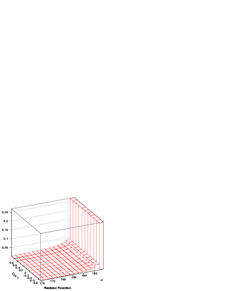
Figure 1: The radiator function $\tilde{R}_{1}\left(s,s^{\prime}\right)$ with $s=\left(200\textrm{ GeV}\right)^{2}$, obtained from the ZFITTER package by extracting it separately for each angular bin for the $\mu^{+}\mu^{-}$ final state.

4 Structure Functions, Leading Log Approximation.

The purpose of this section is to add weight to the empirical observations of the last section by deriving the electron structure function. The idea for a structure function for the electron originates from the paper of Gribov and Lipatov [11]. In the papers of Kuraev, Fadin, Jadach and Skrzypek [6, 9] the authors consider the process of $e^{+}e^{-}$ annihilation as being a Drell-Yan process and exploit the perturbative nature of QED to calculate the electron structure function analytically using the Gribov-Lipatov Altarelli-Parisi equations. This structure function approach represents a leading logarithmic approximation (LLA), this corresponds to assuming near collinear emission of photons from the incoming $e^{+}e^{-}$. The radiator function in the literature is by no means unique. The structure function approach / the leading log approximation, is one way to take into account the effects of ISR. The structure function approach is intuitive, simple and it produces a cross section to better than $0.015$% [7], this alone is a good reason to discuss it. For clarity and completeness we review the results of Kuraev and Fadin (KF) as well as Jadach and Skrzypek (JS) with the help of a combination of papers [6, 7, 9, 10, 12]. In doing this we explicitly confirm (as noted in the introduction of [7]) that no element of the underlying hard scattering process enters this description of ISR and check whether or not it may be applied to the differential cross section as well as the integrated cross section.

The non-singlet structure function $D^{NS}\left(x,s\right)$ corresponds to the probability of finding an electron with longitudinal momentum fraction $x$ ‘inside’ the original on-shell electron at energy scale $\sqrt{s}$. The generic starting point for determining the structure function is Lipatov’s equation (see e.g. [2])

$$D^{NS}\left(x,s\right)=\delta\left(1-x\right)+\int_{m_{e}^{2}}^{s}\frac{{\rm{d}}s_{1}}{s_{1}}\frac{\alpha\left(s_{1}\right)}{2\pi}\int_{x}^{1}\frac{{\rm{d}}x_{1}}{x_{1}}\textrm{ }P\left(x_{1}\right)D^{NS}\left(\frac{x}{x_{1}},s_{1}\right).$$ (4.1)

where $P\left(z\right)$ is the regularized splitting function

$$P\left(x_{1}\right)=\frac{1+x_{1}^{2}}{1-x_{1}}-\delta\left(1-x_{1}\right)\int_{0}^{1}\textrm{d}z\textrm{ }\frac{1+z^{2}}{1-z}.$$ (4.2)

For our purposes a more useful form of the regularized splitting function involves introducing a cut off at $z=1-\epsilon$ where $\epsilon\ll 1$ is very small

$$-\int_{0}^{1}\textrm{d}z\textrm{ }\frac{1+z^{2}}{1-z}=\lim_{\epsilon\rightarrow 0}2\left(\frac{3}{4}+\log\epsilon\right)-2\epsilon+\frac{1}{2}\epsilon^{2}.$$ (4.3)

In this way we can define a different regularized splitting function

$$\textrm{ }P\left(x_{1}\right)=\textrm{ }2\delta\left(1-x_{1}\right)\left(\frac{3}{4}+\log\epsilon\right)+\theta\left(1-\epsilon-x_{1}\right)\frac{1+x_{1}^{2}}{1-x_{1}}.$$ (4.4)

which is finite when integrated over in the limit $\epsilon\rightarrow 0$. Clearly this form is the natural extension of 4.2, in the limit $\epsilon\rightarrow 0$ 4.2 and 4.3 are identical. Henceforth we omit writing $\lim_{\epsilon\rightarrow 0}$ and drop all terms from our calculations which are vanishing in the limit $\epsilon\rightarrow 0$.

Lipatov’s equation 4.1 has an obvious iterative solution, to see this it is convenient to first rewrite the second integral using

$$\int_{0}^{1}\textrm{d}x_{1}\textrm{d}x_{2}\textrm{ }\delta\left(x-x_{1}x_{2}\right)P\left(x_{1}\right)D^{NS}\left(x_{2},s_{1}\right)=\int_{x}^{1}\frac{\textrm{d}x_{1}}{x_{1}}\textrm{ }P\left(x_{1}\right)D^{NS}\left(\frac{x}{x_{1}},s_{1}\right).$$ (4.5)

In addition we approximate the running coupling constant to a constant $\alpha\left(s\right)=\alpha$ and define $\eta\equiv\eta\left(s\right)=\frac{2\alpha}{\pi}\log\frac{s}{m_{e}^{2}}$, $\eta_{i}\equiv\eta\left(s_{i}\right)$ therefore

$$\textrm{d}\eta_{i}=\frac{\textrm{d}s_{i}}{s_{i}}\frac{2\alpha}{\pi}.$$ (4.6)

With these substitutions Lipatov’s equation 4.1 becomes,

$$D^{NS}\left(x,\eta\right)=\delta\left(1-x\right)+\frac{1}{4}\int_{0}^{\eta}\textrm{d}\eta_{1}\int_{0}^{1}\textrm{d}x_{1}\textrm{d}x_{2}\textrm{ }\delta\left(x-x_{1}x_{2}\right)P\left(x_{1}\right)D^{NS}\left(x_{2},\eta_{1}\right)$$ (4.7)

Substituting relation 4.6 into Lipatov’s equation 4.1 and iterating it i.e. substituting $D\left(x_{i},\eta_{i}\right)$as defined by 4.1 back into 4.1 we have an expansion in $\eta$;

$$\begin{array}[]{rcl}D^{NS}\left(x,\eta\right)&=&\delta\left(1-x\right)\\ &+&\frac{1}{4}\int_{0}^{\eta}{\rm{d}}\eta_{1}\int_{0}^{1}{\rm{d}}x_{1}{\rm{d}}x_{2}\textrm{ }\delta\left(x-x_{1}x_{2}\right)P\left(x_{1}\right)\delta\left(1-x_{2}\right)\\ &+&\frac{1}{4}\int_{0}^{\eta}{\rm{d}}\eta_{1}\int_{0}^{1}{\rm{d}}x_{1}{\rm{d}}x_{2}\textrm{ }\delta\left(x-x_{1}x_{2}\right)P\left(x_{1}\right)\frac{1}{4}\int_{0}^{\eta_{1}}{\rm{d}}\eta_{2}\int_{0}^{1}{\rm{d}}x_{3}{\rm{d}}x_{4}\textrm{ }\delta\left(x_{2}-x_{3}x_{4}\right)P\left(x_{3}\right).....\\ &+&{\mathcal{{O}}}\left(\eta^{3}\right)\end{array}.$$ (4.8)

The fact that the integrals $\int_{0}^{\eta_{i}}\textrm{d}\eta_{i}$ are nested, that is to say the upper limit of one integrand is the dummy variable of the one preceding it, results in a sequence of exponential factors $\frac{1}{i!}$ multiplying the terms above. 4.7 is condensed by simple delta function manipulations

$$\begin{array}[]{rl}&D^{NS}\left(x,\eta\right)\\ =&\delta\left(1-x\right)\\ +&1\times\left(\frac{\eta}{4}\right)^{1}P\left(x\right)\\ +&\frac{1}{2}\times\left(\frac{\eta}{4}\right)^{2}\int_{0}^{1}{\rm{d}}x_{1}{\rm{d}}x_{2}\textrm{ }\delta\left(x-x_{1}x_{2}\right)P\left(x_{1}\right)P\left(x_{2}\right)\\ +&\frac{1}{6}\times\left(\frac{\eta}{4}\right)^{3}\int_{0}^{1}{\rm{d}}x_{1}{\rm{d}}x_{2}\textrm{ }\delta\left(x-x_{1}x_{2}\right)P\left(x_{1}\right)\int_{0}^{1}{\rm{d}}x_{3}{\rm{d}}x_{4}\textrm{ }\delta\left(x_{2}-x_{3}x_{4}\right)P\left(x_{3}\right)P\left(x_{4}\right)\\ +&{\mathcal{{O}}}\left(\eta^{4}\right)\end{array}.$$ (4.9)

Denoting the convolution integrals above by

$$\int_{0}^{1}\textrm{d}x_{i}\textrm{d}x_{j}\textrm{ }\delta\left(x-x_{i}x_{j}\right)f\left(x_{i}\right)g\left(x_{j}\right)=f\left(.\right)\otimes g\left(.\right)\left(x\right),$$ (4.10)

equation 4.8 becomes

$$D^{NS}\left(x,s\right)=\delta\left(1-x\right)+\sum_{i=1}^{\infty}\frac{1}{i!}\left(\frac{\eta}{4}\right)^{i}P^{\otimes i}\left(x\right),$$ (4.11)

where

$$P^{\otimes 3}\left(x\right)=\int_{0}^{1}\textrm{d}x_{1}\textrm{d}x_{2}\textrm{ }\delta\left(x-x_{1}x_{2}\right)P\left(x_{1}\right)\int_{0}^{1}\textrm{d}x_{3}\textrm{d}x_{4}\textrm{ }\delta\left(x_{2}-x_{3}x_{4}\right)P\left(x_{3}\right)P\left(x_{4}\right)$$ (4.12)

etc.

The ${\mathcal{{O}}}\left(\eta\right)$ term is simply the regularized splitting function, $\frac{1}{4}\eta P\left(x\right)$. In calculating the ${\mathcal{{O}}}\left(\eta^{2}\right)$ term first we calculate the theta term, we proceed essentially in an identical way to that in which we calculated the regularized splitting function. We calculate a regularized version of this term by taking $x$ to be less than a cut off $x<1-\epsilon$.

$$\begin{array}[]{rl}&\theta\left(1-x-\epsilon\right)\int_{0}^{1}{\rm{d}}x_{1}{\rm{d}}x_{2}\textrm{ }\delta\left(x-x_{1}x_{2}\right)P\left(x_{1}\right)P\left(x_{2}\right)\\ =&\theta\left(1-x-\epsilon\right)4\left(\frac{3}{4}+\log\epsilon\right)^{2}\int_{0}^{1}{\rm{d}}x_{1}{\rm{d}}x_{2}\textrm{ }\delta\left(x-x_{1}x_{2}\right)\delta\left(1-x_{1}\right)\delta\left(1-x_{2}\right)\\ +&\theta\left(1-x-\epsilon\right)2\left(\frac{3}{4}+\log\epsilon\right)\int_{0}^{1-\epsilon}{\rm{d}}x_{1}\int_{0}^{1}{\rm{d}}x_{2}\textrm{ }\delta\left(x-x_{1}x_{2}\right)\delta\left(1-x_{2}\right)\frac{1+x_{1}^{2}}{1-x_{1}}\\ +&\theta\left(1-x-\epsilon\right)2\left(\frac{3}{4}+\log\epsilon\right)\int_{0}^{1}{\rm{d}}x_{1}\int_{0}^{1-\epsilon}{\rm{d}}x_{2}\textrm{ }\delta\left(x-x_{1}x_{2}\right)\textrm{ }\delta\left(1-x_{1}\right)\frac{1+x_{2}^{2}}{1-x_{2}}\\ +&\theta\left(1-x-\epsilon\right)\int_{0}^{1}{\rm{d}}x_{1}\int_{0}^{1}{\rm{d}}x_{2}\delta\left(x-x_{1}x_{2}\right)\textrm{ }\theta\left(1-\epsilon-x_{1}\right)\theta\left(1-\epsilon-x_{2}\right)\frac{1+x_{1}^{2}}{1-x_{1}}\frac{1+x_{2}^{2}}{1-x_{2}}\end{array}$$ (4.13)

The first term is zero due to the cut off we impose on $x$, the other terms are also straightforward to evaluate. As stated earlier small terms ${\mathcal{{O}}}\left(\epsilon\right)$ and above, vanishing in the limit $\epsilon\rightarrow 0$, are dropped. The total theta term obtained with the cut off $x<1-\epsilon$ is

$$\begin{array}[]{rl}&\theta\left(1-\epsilon-x\right)\int_{0}^{1}{\rm{d}}x_{1}{\rm{d}}x_{2}\textrm{ }\delta\left(x-x_{1}x_{2}\right)P\left(x_{1}\right)P\left(x_{2}\right)\\ =&\theta\left(1-x-\epsilon\right)2\left(\frac{1+x^{2}}{1-x}\left(2\log\left(1-x\right)-\log x+\frac{3}{2}\right)+\frac{1}{2}\left(1+x\right)\log x-1+x\right)\end{array}$$ (4.14)

The delta term, analogous to the delta function term in the regularized splitting function 4.4, “soaks up” the divergent part of the term above arising from the limit $x\rightarrow 1$ $\left(\epsilon\rightarrow 0\right)$

$$\begin{array}[]{rl}&-\lim_{\epsilon\rightarrow 0}\int_{0}^{1-\epsilon}{\rm{d}}x\textrm{ }2\left(\frac{1+x^{2}}{1-x}\left(2\log\left(1-x\right)-\log x+\frac{3}{2}\right)+\frac{1}{2}\left(1+x\right)\log x-1+x\right)\\ =&4\left(\left(\frac{3}{4}+\log\epsilon\right)^{2}-\zeta\left(2\right)\right)\end{array}.$$ (4.15)

Finally the full regularized ${\mathcal{{O}}}\left(\eta^{2}\right)$ term is

$$\begin{array}[]{rl}&\frac{1}{2}\left(\frac{\eta}{4}\right)^{2}\int_{0}^{1}{\rm{d}}x_{1}{\rm{d}}x_{2}\textrm{ }\delta\left(x-x_{1}x_{2}\right)P\left(x_{1}\right)P\left(x_{2}\right)\\ =&\left(\frac{\eta}{4}\right)^{2}\delta\left(1-x\right)\left(2\left(\frac{3}{4}+\log\epsilon\right)^{2}-2\zeta\left(2\right)\right)\\ +&\left(\frac{\eta}{4}\right)^{2}\theta\left(1-x-\epsilon\right)\left(\frac{1+x^{2}}{1-x}\left(2\log\left(1-x\right)-\log x+\frac{3}{2}\right)+\frac{1}{2}\left(1+x\right)\log x-1+x\right)\end{array}.$$ (4.16)

The third order term, ${\mathcal{{O}}}\left(\eta^{3}\right)$, is simply

$$\frac{1}{6}\left(\frac{\beta}{4}\right)^{3}\int_{0}^{1}{\rm{d}}x_{1}{\rm{d}}x_{2}\textrm{ }\delta\left(x-x_{1}x_{2}\right)P\left(x_{1}\right)\int_{0}^{1}{\rm{d}}x_{3}{\rm{d}}x_{4}\textrm{ }\delta\left(x_{2}-x_{3}x_{4}\right)P\left(x_{3}\right)P\left(x_{4}\right).$$ (4.17)

Clearly the $\int_{0}^{1}\textrm{d}x_{3}\textrm{d}x_{4}$ part of this term is given by simply substituting in the ${\mathcal{{O}}}\left(\eta^{2}\right)$ term with the replacement, $x\rightarrow x_{2}$. Noting this simplification the resulting calculation is significantly simplified and a long but straightforward sequence of integrations gives the ${\mathcal{{O}}}\left(\eta^{3}\right)$ theta and delta terms of [6].

The Lipatov equation can also be solved analytically in the soft limit $x\rightarrow 0$ by means of a Mellin transformation. The Mellin transform is defined as,

$$\tilde{D}^{NS\left(z\right)}\left(\eta\right)=\int_{0}^{1}{\rm{d}}x\textrm{ }x^{z-1}D^{NS}\left(x,\eta\right)$$ (4.18)

for which the inverse is,

$$D^{NS}\left(x,\eta\right)=\frac{1}{2\pi i}\int_{c-i\infty}^{c+i\infty}{\rm{d}}z\textrm{ }x^{-z}\tilde{D}^{\left(z\right)}\left(\eta\right).$$ (4.19)

The transform exists if $\int_{0}^{1}\textrm{d}x\textrm{ }x^{z-1}\left|D^{NS}\left(x,\eta\right)\right|$ is bounded for some $z>0$ in which case the inverse exists for $c>z$.

Taking the Mellin transform of Lipatov’s equation (4.7) gives

$$\tilde{D}^{NS\left(z\right)}\left(\eta\right)=1+\frac{1}{4}\int_{0}^{\eta}\textrm{d}\eta_{1}\tilde{P}^{\left(z\right)}\tilde{D}^{NS\left(z\right)}\left(\eta_{1}\right)$$ (4.20)

Differentiating the above with respect to $\eta$ gives,

$$\frac{\textrm{d}}{\textrm{d}\eta}\tilde{D}^{NS\left(z\right)}\left(\eta\right)=\frac{1}{4}\tilde{P}^{\left(z\right)}\tilde{D}^{NS\left(z\right)}\left(\eta\right).$$ (4.21)

Integrating this equation one finds a simple expression for the Mellin moments of the structure function in terms of those of the splitting function

$$\tilde{D}^{NS\left(z\right)}\left(\eta\right)=\exp\left(\frac{1}{4}\eta\tilde{P}^{\left(z\right)}\right)$$ (4.22)

where we have used as an initial condition $\tilde{D}^{NS\left(z\right)}\left(m_{e}^{2}\right)=1$. The Mellin moments for the splitting function $\tilde{P}^{\left(z\right)}$ are

$$\tilde{P}^{\left(z\right)}=2\left(\frac{3}{4}+\log\epsilon\right)-\int_{0}^{1-\epsilon}\textrm{d}x\textrm{ }\frac{1-x^{z-1}}{1-x}+\frac{1-x^{z+1}}{1-x}-\frac{2}{1-x}$$ (4.23)

Using the Taylor expansion $\frac{x^{z}}{1-x}=\sum_{n=z}^{\infty}x^{n}$ the integral in 4.23 is trivial, as before we drop terms vanishing in the limit $\epsilon\rightarrow 0$. With a little manipulation of the summations $\tilde{P}^{\left(z\right)}$ becomes,

$$\begin{array}[]{rcl}\tilde{P}^{\left(z\right)}&=&2\left(\frac{3}{4}+\log\epsilon\right)+\int_{0}^{1-\epsilon}\textrm{d}x\textrm{ }x^{z-1}+x^{z}+\frac{2}{1-x}-2\sum_{n=0}^{z}x^{n}\\ &=&-\sum_{n=3}^{z+1}\textrm{ }\frac{1}{n}-\sum_{n=1}^{z-1}\textrm{ }\frac{1}{n}\end{array}.$$ (4.24)

It is worth pointing out that in dropping the terms vanishing in the limit $\epsilon\rightarrow 0$ the cut off $\epsilon$ has now disappeared altogether from the calculation. The Euler function is defined as

$$\psi\left(x\right)=\frac{\textrm{d}}{\textrm{d}x}\log\Gamma\left(x\right)$$ (4.25)

hence,

$$\psi\left(x+1\right)-\psi\left(x\right)=\frac{1}{x}$$ (4.26)

($\Gamma\left(x\right)$ is the Gamma function). In terms of the Euler function,

$$\tilde{P}^{\left(z\right)}=-\psi\left(z+2\right)-\psi\left(z\right)+\psi\left(3\right)+\psi\left(1\right).$$ (4.27)

Using the identity 4.26 again and expanding $\Gamma\left(x\right)$ around $x=1$ we find

$$\tilde{P}^{\left(z\right)}=-\psi\left(z+2\right)-\psi\left(z\right)+\frac{3}{2}-2\gamma.$$ (4.28)

Finally, substituting 4.28 into 4.22, we have an explicit expression for the structure function in terms of its Mellin transform (4.19)

$$D^{NS}\left(x,\eta\right)=\frac{1}{2\pi i}\exp\left(\frac{1}{2}\eta\left(\frac{3}{4}-\gamma\right)\right)\int_{c-i\infty}^{c+i\infty}\textrm{d}z\textrm{ }x^{-z}\exp\left(\frac{1}{4}\eta\left(-\psi\left(z+2\right)-\psi\left(z\right)\right)\right).$$ (4.29)

An analytic expression for the integral above is not known. The integral may be performed in the soft limit $x\rightarrow 1$, this is known as the Gribov approximation. The factor $x^{-z}$ shows that the integral is dominated by large values of $z$. The Euler Gamma function is defined,

$$\Gamma\left(z\right)=\left(z-1\right)!$$ (4.30)

in the large $z$ limit one can approximate the factorial operation by Stirling’s formula $n!\approx\sqrt{2\pi}z^{z+\frac{1}{2}}\exp\left(-z\right)$. In the large $z$ limit we have $\psi\left(z\right)\approx\log z$

$$\Rightarrow D^{NS}\left(x,\eta\right)=\frac{1}{2\pi i}\exp\left(\frac{1}{2}\eta\left(\frac{3}{4}-\gamma\right)\right)\int_{c-i\infty}^{c+i\infty}\textrm{d}z\textrm{ }x^{-z}z^{-\frac{1}{2}\eta}.$$ (4.31)

By substituting $y=z\log x$,

$$D^{NS}\left(x,\eta\right)=\frac{1}{2\pi i}\exp\left(\frac{1}{2}\eta\left(\frac{3}{4}-\gamma\right)\right)\left(\log x\right)^{\frac{1}{2}\eta-1}\int_{c^{\prime}+i\infty}^{c^{\prime}-i\infty}\textrm{d}y\textrm{ }y^{-\frac{1}{2}\eta}\exp\left(-y\right).$$ (4.32)

After the transformation the limits have changed $c+i\infty\rightarrow c\log x+i\infty\log x=c^{\prime}-i\infty$. Importantly $c^{\prime}$ is negative as $\log x<0$ and $c>z>0$ is required for the Mellin transform to exist. The integrand has two obvious singularities, one at $y=0$ and another at $\textrm{Re}\left(y\right)\rightarrow-\infty$ $\left(\textrm{Re}\left(z\right)\rightarrow\infty\right)$. For $\left|y\right|\rightarrow\infty$ and $\textrm{Re}\left(y\right)\neq-\infty$ the integrand is zero, this being the case we can close the integration contour by joining up the two ends at $c^{\prime}+i\infty$ and $c^{\prime}-i\infty$ such that it becomes a hemisphere of radius $\left|y\right|=\infty$ in the $\textrm{Re}\left(y\right)>c^{\prime}$ region of the complex $y-$plane, as the integrand is zero along this addition to the contour. Given the contour is closed in the complex plane we can deform it as we please so long has we keep all poles inside it as its value is given by $2\pi i$ times the residue at the pole, in this case the only pole is at $y=0$. The Hankel contour ${\mathcal{{C_{H}}}}$ in the complex plane is an open contour which comes in along just under the real axis from $+\infty$ goes around the origin and back out to $-\infty$ just above the real axis. We can clearly deform our contour to Hankel’s contour as it contains the origin and no other poles and because our integrand is zero at $\left|y\right|=\infty$ and $\textrm{Re}\left(y\right)\neq-\infty$ we can open the contour again at $\left|y\right|=\infty$ making it exactly the Hankel contour. The integral can then be brought into the form of Hankel’s integral representation of the Gamma function

$$\Gamma\left(\frac{1}{2}\eta\right)^{-1}=-\frac{1}{2\pi i}\int_{{\mathcal{{C_{H}}}}}\textrm{d}y\textrm{ }\left(-y\right)^{-\frac{1}{2}\eta}\exp\left(-y\right).$$ (4.33)

Inserting $1=\left(-1\right)^{-\frac{1}{2}\eta}\left(-1\right)^{+\frac{1}{2}\eta-1}\left(-1\right)^{+1}$ and 4.33 into 4.32 gives

$$D_{Gribov}^{NS}\left(x,\eta\right)=\exp\left(\frac{1}{2}\eta\left(\frac{3}{4}-\gamma\right)\right)\frac{\left(1-x\right)^{\frac{1}{2}\eta-1}}{\Gamma\left(\frac{1}{2}\eta\right)}.$$ (4.34)

(we have used $\lim_{x\rightarrow 1}-\log\left(x\right)=\lim_{x\rightarrow 1}1-x$).

The result of the Gribov approximation constitutes the perturbative result derived earlier extended to all orders with the caveat that it is only valid for the limit $x\rightarrow 1$. To quote Gribov and Lipatov [10] the approximation above “can be considered as a generalization of the Sudakov form factor”. The perturbative structure function calculated earlier has no such constraint on it but is nonetheless a finite order perturbative result. Ideally one wants a single expression for the structure function which tends to the Gribov result at in the soft limit and to the perturbative result away from $x\rightarrow 1$, the desired expression will interpolate between the perturbative structure function and the Gribov approximation. Such interpolation constitutes what is known as exponentiation. Integrating 4.34 over the soft phase space gives,

$$\int_{1-\epsilon}^{1}\textrm{d}x\textrm{ }D_{Gribov}^{NS}\left(x,\eta\right)=\exp\left(\frac{1}{2}\eta\left(\frac{3}{4}-\gamma\right)\right)\frac{\epsilon^{\frac{1}{2}\eta}}{\Gamma\left(1+\frac{1}{2}\eta\right)}.$$ (4.35)

We denote this $D_{Soft}^{NS}\left(\epsilon,\eta\right)$ and rewrite the $\epsilon$ term $\exp\left(\frac{1}{2}\log\epsilon\right)$,

$$D_{Soft}^{NS}\left(\epsilon,\eta\right)=\frac{\exp\left(-\frac{1}{2}\eta\gamma\right)}{\Gamma\left(1+\frac{1}{2}\eta\right)}\exp\left(\frac{1}{2}\eta\left(\frac{3}{4}+\log\epsilon\right)\right).$$ (4.36)

The soft part of the structure function $D_{Soft}^{NS}\left(\epsilon,\eta\right)$ gives an expansion in powers of $\eta$ with coefficients exactly the same as the coefficients of $\eta$ in the delta term obtained earlier by iterating the Lipatov equation, so justifying the earlier quote of Gribov and Lipatov. We have checked this explicitly to ${\mathcal{{O}}}\left(\beta^{3}\right)$. Had we calculated the ${\mathcal{{O}}}\left(\beta^{4}\right)$ delta term with Lipatov’s equation we would see its coefficient is the same as the coefficient of the ${\mathcal{{O}}}\left(\beta^{4}\right)$ term in the expansion of $D_{Soft}^{NS}\left(\epsilon,\eta\right)$. In the perturbative solution the delta terms give the structure function in the $1-\epsilon<x\leq 1$ region. If we were to integrate the delta terms over $1-\epsilon<x\leq 1$ and expand in $\eta$ we would get the same result as we would just expanding $D_{Soft}^{NS}\left(\epsilon,\eta\right)$ up to the same power in $\eta$. Denoting the delta term in the perturbative expansion calculated to ${\mathcal{{O}}}\left(\eta^{i}\right)$ as $\delta\left(1-x\right)\Delta^{\left(i\right)}\left(\epsilon,\eta\right)$ we have,

$$\int_{1-\epsilon}^{1}\textrm{d}x\textrm{ }\delta\left(1-x\right)\Delta^{\left(i\right)}\left(\epsilon,\eta\right)-\int_{1-\epsilon}^{1}\textrm{d}x\textrm{ }D_{Gribov}^{NS}\left(x,\eta\right)\sim{\mathcal{{O}}}\left(\eta^{i+1}\right)$$ (4.37)

this suggests that we modify the structure function by hand to include higher order soft effects by replacing the delta term altogether with $D_{Gribov}^{NS}\left(x,\eta\right)$,

$$\delta\left(1-x\right)\Delta^{\left(i\right)}\left(\epsilon,\eta\right)\rightarrow D_{Gribov}^{NS}\left(x,\eta\right).$$ (4.38)

How does this affect the theta term etc? With this replacement we can safely take the already implied limit $\epsilon\rightarrow 0$, the theta function for the theta term is then replaced by $1$. Then the most obvious thing to do is to demand that, up to the same order in $\eta$, the new structure function is the same as the old purely perturbative one was in the region $0<x<1-\epsilon$ and not care about the terms that are higher order in $\eta$. Expanding in $\eta$ we have

$$\begin{array}[]{rcl}D_{Gribov}^{NS}\left(x,\eta\right)&=&\frac{2}{1-x}\left(\frac{\eta}{4}\right)^{1}\\ &+&\frac{3+4\log\left(1-x\right)}{1-x}\left(\frac{\eta}{4}\right)^{2}\\ &+&\frac{\frac{9}{4}-\frac{3}{4}\pi^{2}+6\log\left(1-x\right)+4\log^{2}\left(1-x\right)}{1-x}\left(\frac{\eta}{4}\right)^{3}\\ &+&{\mathcal{{O}}}\left(\eta^{4}\right)\end{array}.$$ (4.39)

Recall that the Gribov solution is valid in the large $x$ limit. The perturbative solution obtained order by order in $\eta$ by iterating solutions through Lipatov’s equation requires no such approximation. Consequently one expects that the perturbative solution and the Gribov approximation should agree in the limit $x\rightarrow 1$. This is indeed the case, it is easy to verify that the $x\rightarrow 1$ limit of the theta terms obtained in the perturbative case are equal to those obtained in the non-perturbative case. If we denote the $ith$ order in $\eta$ of a quantity by appending superscript $\left(i\right)$ to it we can define an improved structure function

$$D^{\prime NS\left(i\right)}\left(x,\eta\right)=\left\{\begin{array}[]{ll}D_{Gribov}^{NS\left(i\right)}\left(x,\eta\right)+\left(\left.D^{NS\left(i\right)}\left(x,\eta\right)\right|_{\theta-term}-D_{Gribov}^{NS\left(i\right)}\left(x,\eta\right)\right)&0<i\leq 3\\ D_{Gribov}^{NS\left(i\right)}\left(x,\eta\right)&i>3\end{array}\right.$$ (4.40)

i.e.

$$D^{\prime NS}\left(x,\eta\right)=D_{Gribov}^{NS}\left(x,\eta\right)+\sum_{i=0}^{3}\left(\left.D^{NS\left(i\right)}\left(x,\eta\right)\right|_{\theta-term}-D_{Gribov}^{NS\left(i\right)}\left(x,\eta\right)\right).$$ (4.41)

This is the exponentiation prescription of Kuraev and Fadin [9]. The condition on $i$ relates to the order to which the perturbative solution was found, in our case $3$. Applying prescription 4.40 to the perturbative theta terms obtained so far is trivial albeit tedious subtraction, we find agreement with the results in [6, 7]. It is of note that the integral of this function over the range $1-\epsilon\rightarrow\epsilon$ is finite in the limit $\epsilon\rightarrow 0$. The integral is finite because, as stated above, in the divergent $x\rightarrow 1$ limit the theta terms are equal to the corresponding Gribov terms inside the summation, in addition the integral over the all orders Gribov approximation to the left of the sum is finite (see equation 4.36).

An alternative exponentiation prescription is that of Jadach and Ward called YFS exponentiation. Here the only difference is that the Gribov term is extracted from the iterative solution as a factor rather than subtracted as in the Kuraev Fadin exponentiation viz

$$D^{\prime NS\left(i\right)}\left(x,\eta\right)=\left\{\begin{array}[]{ll}\sum_{j+k=i}D_{Gribov}^{NS\left(j\right)}\left(x,\eta\right)\Delta^{\left(k\right)}\left(x,\eta\right)&0<i\leq 3\\ D_{Gribov}^{NS\left(i\right)}\left(x,\eta\right)\Delta^{\left(k\right)}\left(x,\eta\right)&i>3\end{array}\right.,$$ (4.42)

where $\Delta^{\left(k\right)}\left(x,\eta\right)$ is defined by

$$\left.D^{NS\left(i\right)}\left(x,\eta\right)\right|_{\theta-term}=\sum_{j+k=i}D_{Gribov}^{NS\left(j\right)}\left(x,\eta\right)\Delta^{\left(k\right)}\left(x,\eta\right)\textrm{ }\left(1\leq j+k\leq 3,\textrm{ }0\leq k\leq 2\right).$$ (4.43)

This is a system of linear equations that is easily solved for the $\Delta^{\left(k\right)}\left(x,\eta\right)$,

$$\begin{array}[]{rcl}\Delta^{\left(0\right)}\left(x,\eta\right)&=&\frac{\left.D^{NS\left(1\right)}\left(x,\eta\right)\right|_{\theta-term}}{D_{Gribov}^{NS\left(1\right)}\left(x,\eta\right)}\\ \Delta^{\left(1\right)}\left(x,\eta\right)&=&\frac{\left.D^{NS\left(2\right)}\left(x,\eta\right)\right|_{\theta-term}}{D_{Gribov}^{NS\left(1\right)}\left(x,\eta\right)}-\frac{D_{Gribov}^{NS\left(2\right)}\left(x,\eta\right)}{D_{Gribov}^{NS\left(1\right)}\left(x,\eta\right)}\Delta^{\left(0\right)}\left(x,\eta\right)\\ \Delta^{\left(2\right)}\left(x,\eta\right)&=&\frac{\left.D^{NS\left(3\right)}\left(x,\eta\right)\right|_{\theta-term}}{D_{Gribov}^{NS\left(1\right)}\left(x,\eta\right)}-\frac{D_{Gribov}^{NS\left(3\right)}\left(x,\eta\right)}{D_{Gribov}^{NS\left(1\right)}\left(x,\eta\right)}\Delta^{\left(0\right)}\left(x,\eta\right)-\frac{D_{Gribov}^{NS\left(2\right)}\left(x,\eta\right)}{D_{Gribov}^{NS\left(1\right)}\left(x,\eta\right)}\Delta^{\left(1\right)}\left(x,\eta\right)\end{array}$$ (4.44)

giving

$$\begin{array}[]{rl}&D^{\prime NS}\left(x,\eta\right)\\ =&D_{Gribov}^{NS}\left(x,\eta\right)\times\left(\frac{1}{2}\left(1+x\right)^{2}+\frac{1}{16}\left(-2\left(1-x\right)^{2}-\left(1+3x^{2}\right)\log x\right)\eta\right.\\ +&\left.\frac{1}{384}\left(12\left(1-x\right)^{2}+\left(6\left(1-4x+3x^{2}\right)+\left(1+7x^{2}\right)\log x\right)\log x-12\left(1-x\right)^{2}\textrm{Li}_{2}\left(1-x\right)\right)\eta^{2}\right)\end{array}.$$ (4.45)

This is the result given in [6, 7].

To summarize, we have re-derived in this section again the structure functions of Kuraev and Fadin 4.40 and Jadach and Skrzypek. At no point is the underlying hard scattering process referred to, with this approach folding the radiator function with New Physics is just as valid as folding it with the standard model. In addition, within the context of Lipatov’s equation (i.e. for the case of near collinear emission of radiation) the calculations suggest that the factorization of the corrections holds at the level of the differential cross section not just the total cross section. We are seeing this effect in the flatness of the radiator functions we have derived in figure 1. In fact the third order Kuraev-Fadin structure function 4.40 is folded with itself 3.5 and present within ZFITTER as the default setting for the flag higher FOT2 which governs the implementation of higher order radiative corrections. Crucially at this level of approximation the hard scattering interaction is not referred to, this is clearly good news for fits to new physics. Approximations are made in the leading log approximations e.g. the finite order perturbative result nevertheless they have been found to agree very well (KF better than 0.2%, YFS better than ~0.01%) with exact numerical solutions of the Lipatov equation. This would seem to vindicate the use of ISR corrections, the numerical radiator function, derived from ZFITTER and other such packages.

5 The Breakdown of the Simple LLA Structure Function Approach.

In general the standard model predictions obtained from ZFITTER and the other standard model difermion packages allow many more sophisticated radiative corrections to be applied to the process in question besides just ISR. In particular initial state-final state interference (ISR*FSR) effects corresponding to interference between diagrams with bremsstrahlung emitted from initial state particles and diagrams with bremsstrahlung emitted from final state particles, as well as box diagrams resulting from emission and re-absorption of photons, have a significant (~10%) effect at the level of the differential cross section despite having only a negligible (<1%) effect on the total cross section. The radiator functions derived from ZFITTER with these corrections included are shown in figure 2 where they have acquired a significant angular dependence that was not seen in figure 1.

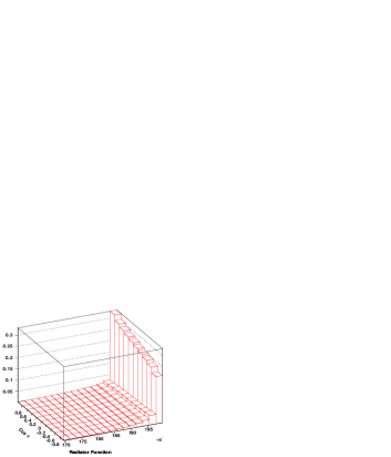
Figure 2: The plot above shows the radiator functions $\tilde{R}_{1}\left(s,s^{\prime}\right)$ with $s=\left(200\textrm{ GeV}\right)^{2}$, obtained from the ZFITTER package by extracting it separately for each angular bin just as in figure 1 but this time including initial state-final state interference effects.

This angular dependence would seem to ruin the argument put forward in 3, which says that these corrections should be independent of the polar angle if in fact they are independent of the hard physics process. It also highlights the weak point in the leading log approximation, the leading log approximation starts to break down for exclusive observables i.e. highly differential quantities and measurements obtained with strong cuts [6]. ISR*FSR interference corrections clearly fall outside the mandate of the structure function / leading log approach which describes ISR effects so well.

In fact the cross section obtained with angular cuts requires two radiator functions. The $\cos\theta$ symmetric and $\cos\theta$ asymmetric parts of the tree level cross section are convoluted separately with different radiator functions and the result added [18, 19, 16]. The cross section in an angular bin $i$ with edges at $c=\cos\theta=c_{i},c_{i+1}$ $\sigma_{i}\left(s,c_{i},c_{i+1}\right)$ is

$$\sigma\left(s,c_{i},c_{i+1}\right)=\int_{c_{i}}^{c_{i+1}}\textrm{d}c\textrm{ }\frac{{\rm{d}}\sigma}{{\rm{d}}c}.$$ (5.1)

Defining the symmetric and asymmetric cross sections $\sigma_{T}\left(s,-c_{i},c_{i}\right)$ and $\sigma_{FB}\left(s,-c_{i},c_{i}\right)$ respectively in the region $-c_{i}<c\leq c_{i}$ as

$$\begin{array}[]{rcl}\sigma_{T}\left(s,-c_{i},c_{i}\right)&=&\frac{1}{2}\left[\int_{0}^{c_{i}}\textrm{d}c\textrm{ }\frac{{\rm{d}}\sigma}{{\rm{d}}c}+\int_{-c_{i}}^{0}\textrm{d}c\textrm{ }\frac{{\rm{d}}\sigma}{{\rm{d}}c}\right]\\ \sigma_{FB}\left(s,-c_{i},c_{i}\right)&=&\frac{1}{2}\left[\int_{0}^{c_{i}}\textrm{d}c\textrm{ }\frac{{\rm{d}}\sigma}{{\rm{d}}}-\int_{-c_{i}}^{0}\textrm{d}c\textrm{ }\frac{{\rm{d}}\sigma}{{\rm{d}}c}\right]\end{array},$$ (5.2)

the cross section in the angular bin is

$$\sigma\left(s,c_{i},c_{i+1}\right)=\sigma_{T}\left(s,-c_{i+1},c_{i+1}\right)+\sigma_{FB}\left(s,-c_{i+1},c_{i+1}\right)-\sigma_{T}\left(s,-c_{i},c_{i}\right)-\sigma_{FB}\left(s,-c_{i},c_{i}\right).$$ (5.3)

In terms of a cross section corrected for radiative effects we have

$$\begin{array}[]{rcl}\sigma_{T}\left(s,-c_{i},c_{i}\right)&=&\int_{s_{min}^{\prime}}^{s}\textrm{d}s^{\prime}\textrm{ }R_{T}\left(s,s^{\prime},c_{i}\right)\sigma_{Tree}\left(s^{\prime}\right)\\ \sigma_{FB}\left(s,-c_{i},c_{i}\right)&=&\int_{s_{min}^{\prime}}^{s}\textrm{d}s^{\prime}\textrm{ }R_{FB}\left(s,s^{\prime},c_{i}\right)\sigma_{Tree}\left(s^{\prime}\right)\end{array}.$$ (5.4)

So far we have assumed

$$R_{T}\left(s,s^{\prime},c_{i}\right)=R_{FB}\left(s,s^{\prime},c_{i}\right),$$ (5.5)

and that to good approximation (3.8),

$$\sigma\left(s,c_{i},c_{i+1}\right)=\int_{s_{min}^{\prime}}^{s}\textrm{d}s^{\prime}\textrm{ }\tilde{R}_{1}\left(s,s^{\prime}\right)\sigma_{Tree}\left(s^{\prime},c_{i},c_{i+1}\right)$$ (5.6)

where, recalling section 3, $\tilde{R}\left(s,s^{\prime}\right)$ is a universally applicable radiator function. According to Bardin et al [19] “Strictly speaking an ansatz like 5.5 is wrong.” In [19] the authors go on to say that near the Z peak the ansatz 5.5 nonetheless gives “excellent agreement with the correct result”. The authors say that this effect is due to the dominant corrections being from soft photons. They go on to say that if an $s^{\prime}$ cut is in use the agreement is even better. We appeal to this soft photon dominance ansatz due to the restrictive $s^{\prime}$ cuts used in obtaining samples to fit with, $\sqrt{s^{\prime}}\geq 0.85\sqrt{s}$, the degree to which it holds is born out by the flatness in $\cos\theta$ of the corrections we derived, $\tilde{R}\left(s,s^{\prime}\right)$ in figure 1. If the corrections were significantly different for the $\cos\theta$ symmetric and asymmetric parts of the differential cross section $\tilde{R}\left(s,s^{\prime}\right)$would not be flat in $\cos\theta$ as we essentially are just dividing the corrected cross section in each angular bin by the born cross section in each angular bin, bin by bin in $s^{\prime}$, the born cross section could not possibly factor out. Prior to considering initial state-final state interference effects there seems to be nothing wrong in using the same radiator function for $c$ even and $c$ odd parts of the cross section, the structure functions we derived describe the radiator function very well.

As you can see in figure 2 the addition of initial state-final state interference effects seem to ruin all our previous hypotheses. Ideally one would hope that just because the radiative corrections have acquired this angular dependence they are still nonetheless essentially universal like the other (ISR) corrections or at least largely process independent in our phase space. Given that we are dealing with box diagrams such factorization seems like wishful thinking.

6 ISR*FSR Universality.

In this section we describe how the ISR*FSR interference corrections, despite giving the naive radiator function an important angular dependence, is nonetheless mostly a universal correction. The ISR*FSR interference corrections for some underlying hard scattering involving the exchange of an unknown particle (???) may be represented at ${\mathcal{{O}}}\left(\alpha^{3}\right)$ by the Feynman diagrams in figures 3 and 4.

Figure 3: ISR*FSR terms in the cross section originate from diagrams with photons emitted from the initial legs and final state legs interfering.

Figure 4: In addition to the bremsstrahlung diagrams in figure 3, at the same order in $\alpha$, ISR*FSR terms in the cross section also originate from diagrams with photons box diagrams interfering with the lowest order diagram.

In subsections 6.1 and 6.2 we will use the Feynman rules of [2] and the kinematic notations of appendix A. In these subsections we will try to maintain an explicit notation. The matrix elements of the two fermion events under discussion at this order have four fermions and hence four spinors in them, $\bar{\nu}_{e}\left(p_{+}\right),\textrm{ }u_{e}\left(p_{-}\right)$ represent the incoming $e^{+}$ and $e^{-}$, $\nu_{f}\left(q_{+}\right),\textrm{ }\bar{u}_{f}\left(q_{-}\right)$ represent the outgoing antifermion and fermion respectively. Given that we are trying to discuss radiative corrections in such a way as to find and highlight any universal features of them it will therefore be useful to denote the born level process generically as

$${\mathcal{{A}}}_{Born}=\bar{\nu}_{e}\left(p_{+}\right)...Hard...\nu_{f}\left(q_{+}\right)$$ (6.1)

where $...Hard...$ is defined to contain the electron and fermion spinors and more importantly, the propagator of the exchanged particle and its couplings to the incoming and outgoing particles (see also equation 6.3). For example in the case of QED we have simply

$$...Hard...=iQ_{e}e\gamma^{\mu}u_{e}\left(p_{-}\right)\frac{-ig_{\mu\nu}}{\left(p_{-}+p_{+}\right)^{2}}\bar{u}_{f}\left(q_{-}\right)iQ_{f}e\gamma^{\nu}.$$ (6.2)

6.1 ${\mathcal{{O}}}\left(\alpha^{3}\right)$ Soft Bremsstrahlung.

The contribution of soft bremsstrahlung corrections to 2-fermion processes are greatly important. By soft bremsstrahlung we mean bremsstrahlung which carries off an amount of energy smaller than the energy resolution of the detector, soft photons carry off a negligible amount of energy. Given that the detector cannot therefore tell the difference between a genuine ${\mathcal{{O}}}\left(\alpha\right)$ process and an ${\mathcal{{O}}}\left(\alpha^{3}\right)$ soft bremsstrahlung correction to it, we must add such contributions to our predicted cross section. The amplitude for a general difermion process with bremsstrahlung emitted from the external positron leg of the diagram (figure 5) will be of the form

Figure 5: Some ${\mathcal{{O}}}\left(\alpha^{3}\right)$ bremsstrahlung correction diagrams.

$${\mathcal{{A}}}_{Brem}=\epsilon_{\lambda}^{*}\left(k\right)\bar{\nu}_{e}\left(p_{+}\right)\left\{iQ_{e}e\gamma^{\lambda}\frac{i\left(-\left(\not p_{+}-\not k\right)+m_{e}\right)}{\left(p_{+}-k\right)^{2}-m_{e}^{2}}\right\}...Hard...\nu_{f}\left(q_{+}\right),$$ (6.3)

with $Q_{e}=-1$ for an electron (generally $Q_{f}$ is the charge on the fermion/antifermion $f$ in units of $e$). If we now work in the limit that $\left|k\right|\rightarrow 0$, $s^{\prime}\rightarrow s$, the soft photon approximation, we see that

$${\mathcal{{A}}}_{Soft}=-Q_{e}e\epsilon_{\lambda}^{*}\left(k\right)\bar{\nu}_{e}\left(p_{+}\right)\gamma^{\lambda}\frac{\not p_{+}-m}{2k.p_{+}}...Hard...\nu_{f}\left(q_{+}\right).$$ (6.4)

Simple $\gamma$ matrix manipulation and the application of the Dirac equation to 6.4 gives

$$\begin{array}[]{rcl}{\mathcal{{A}}}_{soft}&=&-\frac{1}{2k.p_{+}}Q_{e}e\epsilon_{\lambda}^{*}\left(k\right)\bar{\nu}_{e}\left(p_{+}\right)\left(2p_{+}^{\lambda}\right)...Hard...\nu_{f}\left(q_{+}\right)\\ &=&-Q_{e}e\frac{\epsilon^{*}.p_{+}}{k.p_{+}}{\mathcal{{A}}}_{born}\end{array}.$$ (6.5)

From this we see that in the soft photon approximation the bremsstrahlung corrections to the born level process are independent of what that born process is, we have extracted the bremsstrahlung correction as an over all constant factor while staying blissfully ignorant of the underlying process. Hopefully it is clear that these tricks can be employed with the other external legs in considering bremsstrahlung emitted from them in the soft photon approximation giving for bremsstrahlung emitted from the $i$th external leg of the diagram

$${\mathcal{{A}}}_{Soft}^{\left(i\right)}=-Q_{i}e\frac{\epsilon^{*}.p_{i}}{k.p_{i}}{\mathcal{{A}}}_{Born}$$ (6.6)

where $p_{i}$ denotes the momentum of the external leg. Consequently, taking into account the bremsstrahlung emitted from all different legs we find the matrix element

$${\mathcal{{A}}}_{Soft}^{\dagger}{\mathcal{{A}}}_{Soft}=\sum_{i,j}Q_{i}Q_{j}e^{2}\frac{\left(\epsilon.p_{i}\right)\left(\epsilon^{*}.p_{j}\right)}{\left(k.p_{i}\right)\left(k.p_{j}\right)}{\mathcal{{A}}}_{Born}^{\dagger}{\mathcal{{A}}}_{Born}.$$ (6.7)

Summing fermion spins and polarizations of the photon $\left(\sum_{pols}\epsilon^{\mu}\epsilon^{*\nu}=-g^{\mu\nu}\right)$ and inserting the phase space and flux factors factors gives in the $k\approx 0$ soft photon approximation

$$\textrm{d}\sigma=-\frac{\alpha}{4\pi^{2}}\sum_{i,j}Q_{i}Q_{j}p_{i}.p_{j}\frac{{\rm{d}}^{3}k}{k_{0}}\frac{1}{\left(k.p_{i}\right)\left(k.p_{j}\right)}\textrm{d}\sigma_{Born}.$$ (6.8)

The soft photon cross section is the contribution to the cross section from soft photons where soft photons were defined earlier as being those low enough in energy to render the bremsstrahlung process indistinguishable from the tree level process, we denote this energy $\omega$, the soft photon cut-off. Integrating over the final state phase space of the soft photon we have

$$\textrm{d}\sigma_{Soft}=-\frac{\alpha}{\pi}\sum_{i,j}Q_{i}Q_{j}p_{i}.p_{j}\left(\frac{1}{4\pi}\int_{\left|\vec{k}\right|<\omega}\frac{{\rm{d}}^{3}\vec{k}}{k_{0}}\frac{1}{\left(k.p_{i}\right)\left(k.p_{j}\right)}\right)\textrm{d}\sigma_{Born}.$$ (6.9)

Note that this differential cross section contains contributions from pairs of diagrams which constitute initial state-final state interference. This would appear to be the desired result, the radiative corrections are factorized from the hard scattering process at the level of the differential cross section.

On its own the result 6.9 arguably does not make much sense as the phase space integral

$$\frac{1}{4\pi}\int_{\left|\vec{k}\right|<\omega}\frac{{\rm{d}}^{3}\vec{k}}{k_{0}}\frac{1}{\left(k.p_{i}\right)\left(k.p_{j}\right)}$$ (6.10)

is infrared divergent, as $k\rightarrow 0$ $\textrm{d}\sigma\rightarrow\infty$. The infrared divergence of the ISR*FSR bremsstrahlung contribution actually cancels an infrared divergence from the ISR*FSR box diagrams. The phase space integral must be expressed in a form whereby we can add the bremsstrahlung and box contributions to cancel the divergences before we can fully assess the universality of the ISR*FSR interference. We have treated the divergence with dimensional regularization. We replace all four dimensional dependence with the usual prescription $4\rightarrow n=4+\epsilon^{\prime}$

$$\frac{1}{4\pi}\int_{\left|\vec{k}\right|<\omega}\frac{{\rm{d}}^{3}\vec{k}}{k_{0}}\frac{1}{\left(k.p_{i}\right)\left(k.p_{j}\right)}\rightarrow\frac{1}{4\pi}\mu^{N}\int_{\left|\vec{k}\right|<\omega}\frac{{\rm{d}}^{n-1}\vec{k}}{k_{0}}\frac{1}{\left(k.p_{i}\right)\left(k.p_{j}\right)}.$$ (6.11)

The factor $\mu^{N}$ is introduced to keep the overall mass dimensions of the integral the same as they were before extending to $N$ dimensions. $\mu^{N}$ has mass dimensions $\left[\mu^{N}\right]=N$ i.e. $N=-\epsilon^{\prime}$ i.e. 6.11 is

$$\frac{1}{4\pi}\left(\frac{1}{\mu}\right)^{\epsilon^{\prime}}\int_{\left|\vec{k}\right|<\omega}\frac{{\rm{d}}^{\epsilon^{\prime}+3}\vec{k}}{k_{0}}\frac{1}{\left(k.p_{i}\right)\left(k.p_{j}\right)}.$$ (6.12)

This photon phase space integral is technical and not so illuminating for our present discussion so we shall confine it to appendix B. After completing the integral the contribution to the differential cross section from ${\mathcal{{O}}}\left(\alpha^{3}\right)$ soft bremsstrahlung diagrams is found to be

$$\textrm{d}\sigma_{Soft,Int}=\frac{2\alpha}{\pi}\left[\left(\frac{1}{\hat{\epsilon}}+\log\left(\frac{4\omega^{2}}{\mu^{2}}\right)\right)\log\left(\frac{t}{u}\right)-\textrm{Li}_{2}\left(1+\frac{s}{t}\right)+\textrm{Li}_{2}\left(1+\frac{s}{u}\right)\right]\textrm{d}\sigma_{Born}.$$ (6.13)

This is the universal soft photon bremsstrahlung correction to the differential cross section from ISR*FSR interference. Left as it is above, the correction to the differential cross section is infrared divergent, there are terms ${\mathcal{{O}}}\left(\epsilon^{\prime-1}\right)$ and the limit $\epsilon^{\prime}\rightarrow 0$ must be taken to return to four dimensional Minkowski space. For our purposes the essential feature of this result is that the radiative correction is factorized from / independent of the new physics exchange process.

6.2 ${\mathcal{{O}}}\left(\alpha^{3}\right)$ Virtual Diagrams.

The infrared divergences $\left(\frac{1}{\hat{\epsilon}}\right)$ in the soft bremsstrahlung result are well known to be physical, that is to say that they are a real part of the theory as opposed to the ultraviolet divergences encountered in renormalization which are a consequence of our ignorance of short distance physics, likewise the infrared divergences cannot be subtracted ad hoc. The infrared divergences due to the emission of soft photons do however cancel against the corresponding virtual diagrams, it is a well known fact that the soft photon contribution to the cross section from initial state bremsstrahlung cancels against a corresponding infrared divergence from the corresponding vertex diagram which involves emitting a photon from one initial state leg and absorbing it on the other. Likewise the initial state-final state interference cross section arising from the interference of initial and final state bremsstrahlung diagrams does not make much sense on its own, it must be added to the corresponding virtual graph. The virtual graph for ISR*FSR bremsstrahlung is by analogy to the case of initial state bremsstrahlung the one formed by taking the photon emitted from an initial state fermion and joining it to a final state fermion. This gives the two diagrams of figure 6.

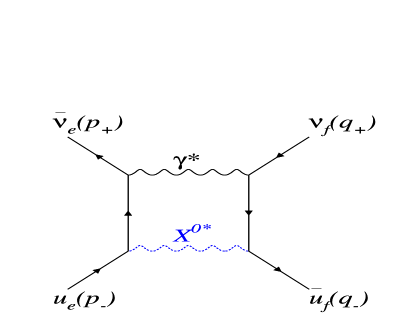
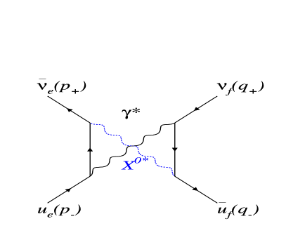
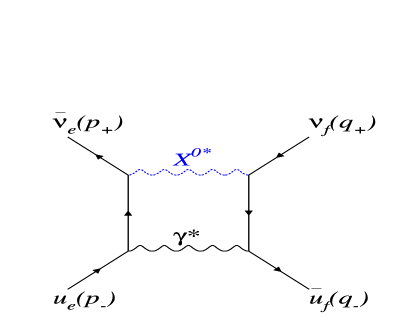
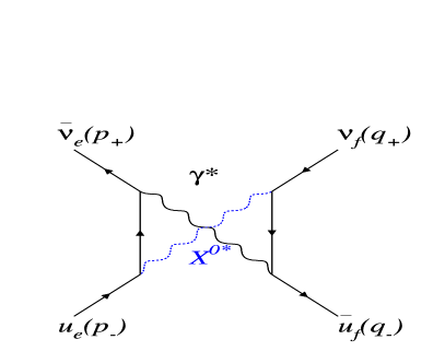
Figure 6: The box diagrams contributing to the ISR*FSR interference cross section. On the left hand side we have direct box diagrams, from top to bottom these are represented by amplitudes ${\mathcal{{A}}}_{D1}$ and ${\mathcal{{A}}}_{D2}$ respectively. On the right hand side we have crossed box diagrams, from top to bottom these are represented by amplitudes ${\mathcal{{A}}}_{C1}$ and ${\mathcal{{A}}}_{C2}$ respectively.

At ${\mathcal{{O}}}\left(\alpha^{3}\right)$ these diagrams only contribute by their interference with the tree level (hard) process. Unlike the soft bremsstrahlung corrections the ISR*FSR box diagrams do not simply represent multiplicative corrections to the born level amplitude. These diagrams were studied in the the hope that, though they do not fall under the banner of universal radiative corrections, they may have some component which is universal. It is quite easy to show that the box diagrams have universal, factorizable corrections. The tricks previously applied to the soft bremsstrahlung diagrams also work, to some degree, with box diagrams (provided there is an internal photon). Let us write down the amplitude for the first direct box diagram in figure 6, were we feign ignorance of the couplings and propagator of the $X^{0}$ boson. We denote the couplings associated of $X^{0}$ some particle $A$ as ${\mathcal{{C}}}_{A}$ and propagator contributions to the numerator as ${\mathcal{{P}}}_{X^{0}}$. We assume the denominator of the propagator is the usual $\left(k^{2}-m_{X}^{2}\right)$ form (for an $X^{0}$ particle four momentum $k$ and mass $m_{X}$). The couplings can be considered to have Dirac and Lorentz indices, the Dirac indices are contracted with the rest of the Dirac algebra in the numerator and the Lorentz indices are contracted with those in ${\mathcal{{P}}}_{X^{0}}$. With these notations ${\mathcal{{P}}}_{X^{0}}...{\mathcal{{C}}}_{e}u\left(p_{-}\right)\bar{u}\left(p_{+}\right){\mathcal{{C}}}_{f}.../\left(s^{2}-m_{X}^{2}\right)$ corresponds to $...Hard...$ in the case of the soft bremsstrahlung. Finally we shall assume the interaction is charge conjugation invariant i.e. ${\mathcal{{C}}}_{A}=-{\mathcal{{C}}}_{\bar{A}}$. The amplitudes for the diagrams in figure 6 are then

$$\begin{array}[]{rcl}{\mathcal{{A}}}_{D1}&=&-ie^{2}\int\frac{{\rm{d}}^{4}k}{\left(2\pi\right)^{4}}\textrm{ }{\mathcal{{P}}}_{X^{0}}\frac{\bar{\nu}\left(p_{+}\right)\gamma^{\mu}\left(-{\not k}-\not p_{+}+m_{e}\right){\mathcal{{C}}}_{e^{-}}u\left(p_{-}\right)\bar{u}\left(q_{-}\right){\mathcal{{C}}}_{f}\left(-{\not k}-\not q_{+}+m_{f}\right)\gamma_{\mu}\nu\left(q_{+}\right)}{k^{2}\left(k^{2}+2k.p_{+}\right)\left(k^{2}+2k.q_{+}\right)\left(k^{2}+s+2k.\left(p_{+}+p_{-}\right)-m_{X}^{2}\right)}\\ {\mathcal{{A}}}_{D2}&=&-ie^{2}\int\frac{{\rm{d}}^{4}k}{\left(2\pi\right)^{4}}\textrm{ }{\mathcal{{P}}}_{X^{0}}\frac{\bar{\nu}\left(p_{+}\right){\mathcal{{C}}}_{e^{+}}\left(\not k+\not p_{-}+m_{e}\right)\gamma^{\mu}u\left(p_{-}\right)\bar{u}\left(q_{-}\right)\gamma_{\mu}\left(\not k+\not q_{-}+m_{f}\right){\mathcal{{C}}}_{\bar{f}}\nu\left(q_{+}\right)}{k^{2}\left(k^{2}+2k.p_{-}\right)\left(k^{2}+2k.q_{-}\right)\left(k^{2}+s+2k.\left(p_{+}+p_{-}\right)-m_{X}^{2}\right)}\\ {\mathcal{{A}}}_{C1}&=&+ie^{2}\int\frac{{\rm{d}}^{4}k}{\left(2\pi\right)^{4}}\textrm{ }{\mathcal{{P}}}_{X^{0}}\frac{\bar{\nu}\left(p_{+}\right){\mathcal{{C}}}_{e^{+}}\left(\not k+\not p_{-}+m_{e}\right)\gamma^{\mu}u\left(p_{-}\right)\bar{u}\left(q_{-}\right){\mathcal{{C}}}_{f}\left(-{\not k}-\not q_{+}+m_{f}\right)\gamma_{\mu}\nu\left(q_{+}\right)}{k^{2}\left(k^{2}+2k.p_{-}\right)\left(k^{2}+2k.q_{+}\right)\left(k^{2}+s+2k.\left(p_{+}+p_{-}\right)-m_{X}^{2}\right)}\\ {\mathcal{{A}}}_{C2}&=&+ie^{2}\int\frac{{\rm{d}}^{4}k}{\left(2\pi\right)^{4}}\textrm{ }{\mathcal{{P}}}_{X^{0}}\frac{\bar{\nu}\left(p_{+}\right)\gamma^{\mu}\left(-{\not k}-\not p_{+}+m_{e}\right){\mathcal{{C}}}_{e^{-}}u\left(p_{-}\right)\bar{u}\left(q_{-}\right)\gamma_{\mu}\left(\not k+\not q_{-}+m_{f}\right){\mathcal{{C}}}_{\bar{f}}\nu\left(q_{+}\right)}{k^{2}\left(k^{2}+2k.p_{+}\right)\left(k^{2}+2k.q_{-}\right)\left(k^{2}+s+2k.\left(p_{+}+p_{-}\right)-m_{X}^{2}\right)}\end{array},$$ (6.14)

where we have defined the loop momentum in each case such that it flows counter-clockwise with the $X^{0}$ propagator carrying momentum $k+p_{+}+p_{-}$i.e. the propagator is the same in each diagram. We have defined the loop momentum $k$ such that in each diagram it is the photon four momentum flowing into the incoming antifermion line. Firstly condense the numerator as much as possible. The ${\not p}$ terms in the numerator may be quickly got rid of by anticommuting them so that the on-shell Dirac equation may be used. Considering the left hand side of the numerator of ${\mathcal{{A}}}_{D1}$

$$\begin{array}[]{rl}&\bar{\nu}\left(p_{+}\right)\gamma^{\mu}\left(-{\not k}-{\not p_{+}}+m_{e}\right)...\\ =&e\bar{\nu}\left(p_{+}\right)\left(-\gamma^{\mu}{\not k}+2p_{+}^{\mu}\right)...\end{array}.$$ (6.15)

Using the same techniques on the right hand side of the various numerators the amplitude can be simplified to

$$\begin{array}[]{rcl}{\mathcal{{A}}}_{D1}&=&-ie^{2}\int\frac{{\rm{d}}^{4}k}{\left(2\pi\right)^{4}}\textrm{ }{\mathcal{{P}}}_{X^{0}}\frac{\bar{\nu}\left(p_{+}\right)\left(\gamma^{\mu}\not k+2p_{+}^{\mu}\right){\mathcal{{C}}}_{e^{-}}u\left(p_{-}\right)\bar{u}\left(q_{-}\right){\mathcal{{C}}}_{f}\left(\not k\gamma_{\mu}+2q_{+\mu}\right)\nu\left(q_{+}\right)}{k^{2}\left(k^{2}+2k.p_{+}\right)\left(k^{2}+2k.q_{+}\right)\left(k^{2}+s+2k.\left(p_{+}+p_{-}\right)-m_{X}^{2}\right)}\\ {\mathcal{{A}}}_{D1}&=&-ie^{2}\int\frac{{\rm{d}}^{4}k}{\left(2\pi\right)^{4}}\textrm{ }{\mathcal{{P}}}_{X^{0}}\frac{\bar{\nu}\left(p_{+}\right){\mathcal{{C}}}_{e^{-}}\left(\not k\gamma^{\mu}+2p_{-}^{\mu}\right)u\left(p_{-}\right)\bar{u}\left(q_{-}\right)\left(\gamma_{\mu}\not k+2q_{-\mu}\right){\mathcal{{C}}}_{f}\nu\left(q_{+}\right)}{k^{2}\left(k^{2}+2k.p_{-}\right)\left(k^{2}+2k.q_{-}\right)\left(k^{2}+s+2k.\left(p_{+}+p_{-}\right)-m_{X}^{2}\right)}\\ {\mathcal{{A}}}_{C1}&=&+ie^{2}\int\frac{{\rm{d}}^{4}k}{\left(2\pi\right)^{4}}\textrm{ }{\mathcal{{P}}}_{X^{0}}\frac{\bar{\nu}\left(p_{+}\right){\mathcal{{C}}}_{e^{-}}\left(\not k\gamma^{\mu}+2p_{-}^{\mu}\right)u\left(p_{-}\right)\bar{u}\left(q_{-}\right){\mathcal{{C}}}_{f}\left(\not k\gamma_{\mu}+2q_{+\mu}\right)\nu\left(q_{+}\right)}{k^{2}\left(k^{2}+2k.p_{-}\right)\left(k^{2}+2k.q_{+}\right)\left(k^{2}+s+2k.\left(p_{+}+p_{-}\right)-m_{X}^{2}\right)}\\ {\mathcal{{A}}}_{C2}&=&+ie^{2}\int\frac{{\rm{d}}^{4}k}{\left(2\pi\right)^{4}}\textrm{ }{\mathcal{{P}}}_{X^{0}}\frac{\bar{\nu}\left(p_{+}\right)\left(\gamma^{\mu}\not k+2p_{+}^{\mu}\right){\mathcal{{C}}}_{e^{-}}u\left(p_{-}\right)\bar{u}\left(q_{-}\right)\left(\gamma_{\mu}\not k+2q_{-\mu}\right){\mathcal{{C}}}_{f}\nu\left(q_{+}\right)}{k^{2}\left(k^{2}+2k.p_{+}\right)\left(k^{2}+2k.q_{-}\right)\left(k^{2}+s+2k.\left(p_{+}+p_{-}\right)-m_{X}^{2}\right)}\end{array}.$$ (6.16)

Assuming that the couplings $\left({\mathcal{{C}}}_{e/f}\right)$and numerator of the $X^{0}$ propagator ${\mathcal{{P}}}_{X^{0}}$ do not depend on the loop momentum we can decompose the amplitudes into tensor $\left(T_{\alpha\beta}\right)$, vector $\left(V_{\alpha}\right)$ and scalar $\left(S\right)$ loop integrals according to the number of powers of $k$ in the numerator

$$\begin{array}[]{rcl}{\mathcal{{A}}}_{D1}&=&-ie^{2}\bar{\nu}\left(p_{+}\right)\gamma^{\mu}\gamma^{\alpha}...\gamma^{\beta}\gamma_{\mu}\nu\left(q_{+}\right)\times T_{\alpha\beta}\\ &&-ie^{2}\bar{\nu}\left(p_{+}\right)\left(\gamma^{\mu}\gamma^{\alpha}...2q_{+\mu}+2p_{+}^{\mu}...\gamma^{\alpha}\gamma_{\mu}\right)\nu\left(q_{+}\right)\times V_{\alpha}\\ &&-4ie^{2}\left(p_{+}.q_{+}\right)\bar{\nu}\left(p_{+}\right)...\nu\left(q_{+}\right)\times S\end{array},$$ (6.17)

where

$$\begin{array}[]{lcl}T_{\alpha\beta}&=&\int\frac{{\rm{d}}^{4}k}{\left(2\pi\right)^{4}}\frac{k_{\alpha}k_{\beta}}{k^{2}\left(\left(k+p_{+}\right)^{2}-m_{e}^{2}\right)\left(\left(k+q_{+}\right)^{2}-m_{f}^{2}\right)\left(\left(k+p_{+}+p_{-}\right)^{2}-m_{X}^{2}\right)}\\ V_{\alpha}&=&\int\frac{{\rm{d}}^{4}k}{\left(2\pi\right)^{4}}\frac{k_{\alpha}}{k^{2}\left(\left(k+p_{+}\right)^{2}-m_{e}^{2}\right)\left(\left(k+q_{+}\right)^{2}-m_{f}^{2}\right)\left(\left(k+p_{+}+p_{-}\right)^{2}-m_{X}^{2}\right)}\\ S&=&\int\frac{{\rm{d}}^{4}k}{\left(2\pi\right)^{4}}\frac{1}{k^{2}\left(\left(k+p_{+}\right)^{2}-m_{e}^{2}\right)\left(\left(k+q_{+}\right)^{2}-m_{f}^{2}\right)\left(\left(k+p_{+}+p_{-}\right)^{2}-m_{X}^{2}\right)}\end{array}$$ (6.18)

and ${\mathcal{{C}}}_{e^{-}}u\left(p_{-}\right)\bar{u}\left(q_{-}\right){\mathcal{{C}}}_{f}$ has been replaced with “$...$” for brevity. We can see that the scalar term in the amplitude of 6.17 is a factor multiplied by the born scattering amplitude of the $X^{0}$particle

$$2it\times e^{2}\times S\times\left(s-m_{X}^{2}\right)\times\left(\frac{\bar{\nu}\left(p_{+}\right){\mathcal{{C}}}_{e^{-}}u\left(p_{-}\right)\bar{u}\left(q_{-}\right){\mathcal{{C}}}_{f}\nu\left(q_{+}\right)}{s-m_{X}^{2}}\right)=2it\times e^{2}\times S\times\left(s-m_{X}^{2}\right)\times{\mathcal{{A}}}_{Born}.$$ (6.19)

The numerator algebra has given a universal factor which multiplies the tree level numerator algebra $4\left(p_{+}.q_{+}\right)=-2t$ however the same is not true of the denominator. The factor $S\times\left(s-m_{X}^{2}\right)$ depends on the underlying hard scattering process through the dependence of $S$ on $m_{X}$, the mass of the exchanged particle. Using the on mass shell relations we can rewrite the denominator of the integrals in the $\left|k\right|\rightarrow 0$ limit as

$$\begin{array}[]{rl}&\lim_{\left|k\right|\rightarrow 0}\frac{1}{k^{2}\left(\left(k+p_{+}\right)^{2}-m_{e}^{2}\right)\left(\left(k+q_{+}\right)^{2}-m_{f}^{2}\right)\left(\left(k+p_{+}+p_{-}\right)^{2}-m_{X}^{2}\right)}\\ =&\frac{1}{k^{2}\left(2k.p_{+}\right)\left(2k.q_{+}\right)\left(s-m_{X}^{2}\right)}\end{array}.$$ (6.20)

By trivially counting powers of $\left|k\right|$ we see that in limit $\left|k\right|\rightarrow 0$ the tensor integral goes as $\int\textrm{d}\left|k\right|\left|k\right|$, the vector integral goes as $\int\textrm{d}\left|k\right|$ and the scalar integral as $\int\textrm{d}\left|k\right|\left|k\right|^{-1}$. Consequently the scalar integral is infrared divergent and the other integrals are infrared finite. Simple power counting also shows that all of the integrals are finite in the ultraviolet limit $\left|k\right|\rightarrow\infty$. Expanding the last bracket in the denominator we can write,

$$S=\int\frac{{\rm{d}}^{4}k}{\left(2\pi\right)^{4}}\frac{1}{k^{2}\left(\left(k+p_{+}\right)^{2}-m_{e}^{2}\right)\left(\left(k+q_{+}\right)^{2}-m_{f}^{2}\right)\left(k^{2}+s+2k.\left(p_{+}+p_{-}\right)-m_{X}^{2}\right)}.$$ (6.21)

In the infrared divergent $\left|k\right|\rightarrow 0$ limit we can rewrite the last part of the denominator

$$\left(k^{2}+s+2k.\left(p_{+}+p_{-}\right)-m_{X}^{2}\right)=\left(s-m_{X}^{2}\right),$$ (6.22)

therefore the radiative correction factor in the scalar integral term

$$2it\times e^{2}\times S\times\left(s-m_{X}^{2}\right),$$ (6.23)

has a divergent piece which is universal because the constant factor $\left(s-m_{X}^{2}\right)$ in 6.23 cancels that which appears in the divergent limit of 6.21. We can perhaps express this result in a better way writing

$$\frac{\left(s-m_{X}^{2}\right)}{\left(k^{2}+2k.\left(p_{+}+p_{-}\right)+s-m_{X}^{2}\right)}=1-\frac{k^{2}+2k.\left(p_{+}+p_{-}\right)}{\left(k^{2}+2k.\left(p_{+}+p_{-}\right)+s-m_{X}^{2}\right)},$$ (6.24)

which makes the scalar integral term equal to

$$\begin{array}[]{rcl}2it\times e^{2}\times S\times\left(s-m_{X}^{2}\right)&=&\int\frac{{\rm{d}}^{4}k}{\left(2\pi\right)^{4}}\frac{2it\times e^{2}}{k^{2}\left(\left(k+p_{+}\right)^{2}-m_{e}^{2}\right)\left(\left(k+q_{+}\right)^{2}-m_{f}^{2}\right)}\\ &-&\int\frac{{\rm{d}}^{4}k}{\left(2\pi\right)^{4}}\frac{2it\times e^{2}\times\left(k^{2}+2k.\left(p_{+}+p_{-}\right)\right)}{k^{2}\left(\left(k+p_{+}\right)^{2}-m_{e}^{2}\right)\left(\left(k+q_{+}\right)^{2}-m_{f}^{2}\right)\left(k^{2}+s+2k.\left(p_{+}+p_{-}\right)-m_{X}^{2}\right)}\end{array}.$$ (6.25)

The first term on the right hand side of 6.25 is universal, the terms in the denominator correspond to the photon propagator and two fermion propagators and the $-2t$ in the numerator came from the universal part of the numerator algebra. The second term on the right hand side of 6.25 clearly depends on the hard scattering process (note the $m_{X}$ terms), it is actually a vector and a tensor loop integral. The universal term goes as $\int\textrm{d}\left|k\right|\left|k\right|^{-1}$ in the $\left|k\right|\rightarrow 0$ limit while the other term goes as $\int\textrm{d}\left|k\right|$ i.e. only the universal part of the scalar integral is infrared divergent. The degree to which the box diagram corrections are universal depends on how big the first integral is in 6.25 relative to the other terms. If we denote the universal part of the scalar integral coming from the denominator of the amplitude

$$S_{U}\left(p_{+},q_{+}\right)=\int\frac{{\rm{d}}^{4}k}{\left(2\pi\right)^{4}}\frac{1}{k^{2}\left(\left(k+p_{+}\right)^{2}-m_{e}^{2}\right)\left(\left(k+q_{+}\right)^{2}-m_{f}^{2}\right)},$$ (6.26)

we can then rewrite the amplitude 6.17

$$\begin{array}[]{rcl}{\mathcal{{A}}}_{D1}&=&-ie^{2}\bar{\nu}\left(p_{+}\right)\gamma^{\mu}\gamma^{\alpha}...\gamma^{\beta}\gamma_{\mu}\nu\left(q_{+}\right)T_{\alpha\beta}-2ie^{2}tT_{\alpha}^{\alpha}{\mathcal{{A}}}_{Born}\\ &&-ie^{2}\bar{\nu}\left(p_{+}\right)\left(\gamma^{\mu}\gamma^{\alpha}...2q_{+\mu}+2p_{+}^{\mu}...\gamma^{\alpha}\gamma_{\mu}\right)\nu\left(q_{+}\right)V_{\alpha}-4ie^{2}tV.\left(p_{+}+p_{-}\right){\mathcal{{A}}}_{Born}\\ &&+2ie^{2}tS_{U}\left(p_{+},q_{+}\right){\mathcal{{A}}}_{Born}\end{array}.$$ (6.27)

where “$...$” represents ${\mathcal{{C}}}_{e^{-}}u\left(p_{-}\right)\bar{u}\left(q_{-}\right){\mathcal{{C}}}_{f}$. Hopefully it is clear that the decomposition of such scalar integrals into a universal part and non-universal part is as general as propagators with denominators of the form $p^{2}-m^{2}$, that is to say no matter what $X^{0}$is we will always find a term $S_{U}$ 6.26.

We can repeat this process with the other diagrams (figure 6) in exactly the same way, in each case we have the generic result that the radiative correction from ISR*FSR box diagrams factorizes from the tree level process in the infrared divergent part of the scalar loop integral. Referring back to 6.16 we see that the other topologies of the process give the following scalar terms

$$\begin{array}[]{rcl}\left.{\mathcal{{A}}}_{D1}\right|_{Scalar}&=&+2ie^{2}tS_{U}\left(p_{+},q_{+}\right){\mathcal{{A}}}_{Born}\\ \left.{\mathcal{{A}}}_{D2}\right|_{Scalar}&=&+2ie^{2}tS_{U}\left(p_{-},q_{-}\right){\mathcal{{A}}}_{Born}\\ \left.{\mathcal{{A}}}_{C1}\right|_{Scalar}&=&-2ie^{2}uS_{U}\left(p_{-},q_{+}\right){\mathcal{{A}}}_{Born}\\ \left.{\mathcal{{A}}}_{C2}\right|_{Scalar}&=&-2ie^{2}uS_{U}\left(p_{+},q_{-}\right){\mathcal{{A}}}_{Born}\end{array}.$$ (6.28)

Again we have found what we are looking for, factorization of the radiative corrections. The ideal result, namely that the differential cross section due to ISR*FSR box diagrams interfering with the tree level process is of the form

$$\textrm{d}\sigma_{Box}=\textrm{Universal Factor}\times\textrm{d}\sigma_{Born},$$ (6.29)

i.e. exactly factorizable requires that the vector and tensor integral terms as well as the non-universal parts of $S$ are negligible relative to the infrared divergent, universal piece of $S$. Clearly an exact factorization is impossible, factorization will only ever occur to some degree. The question then becomes, is a good degree of factorization possible and generic? Requiring a universally good degree of factorization means that the factorizable part of the amplitude must somehow dominate all of the other parts. It does not seem improbable that this be the case as the universal correction we are interested in always corresponds to an infrared divergence, in fact it corresponds to the only divergence, infrared or otherwise. We shall briefly postpone the discussion regarding the relative sizes of the various contributions to $\textrm{d}\sigma_{Box}$ to discuss an initial simplifying assumption.

It is important to note that some of the new physics $X^{0}$ particles which we hope to apply this analysis to will have momentum dependent couplings e.g. gravitons (gravitons couple to the energy momentum tensor). Another, more pertinent point is that bosonic propagators generically contribute polynomials in the momentum of the particle they represent to the numerator as well as the denominator of the amplitude. This does not change our current analysis except at the point of decomposition into scalar vector and tensor integrals 6.17 as gravitons will give ${\mathcal{{C}}}_{e^{-}},\textrm{ }{\mathcal{{C}}}_{f}$ and ${\mathcal{{P}}}_{X^{0}}$ then have a dependence on the loop momentum. In this case the same decomposition can be done into scalar, vector and tensor integrals and crucially one finds that the scalar term is the same as in equation 6.27. To see this all one has to do is simply multiply out any $k$ dependence in ${\mathcal{{P}}}_{X^{0}},\textrm{ }{\mathcal{{C}}}_{e^{-}},\textrm{ }{\mathcal{{C}}}_{f}$ i.e. decompose ${\mathcal{{P}}}_{X^{0}},\textrm{ }{\mathcal{{C}}}_{e^{-}},\textrm{ }{\mathcal{{C}}}_{f}$ into scalar, vector bits etc. Another way to understand this is to recall that the scalar part is infrared divergent and the momentum in the photon in our diagrams is just $k$ the loop momentum, so naively one can think of the photon line in the diagrams as vanishing in the infrared divergent limit. Thus even in the case where there is a non-trivial dependence of the couplings and propagator of $X^{0}$ on the loop momentum the generic infrared term still occurs, essentially one just has to expand in the loop momentum. In the case of momentum dependence of the couplings etc the tensor integrals will naturally involve tensors of higher rank than just two i.e. we will have tensor integrals of the form

$$\int\frac{\textrm{d}^{4}k}{\left(2\pi\right)^{4}}\frac{k_{\alpha}k_{\beta}k_{\gamma}...}{k^{2}\left(\left(k+p_{+}\right)^{2}-m_{e}^{2}\right)\left(\left(k+q_{+}\right)^{2}-m_{f}^{2}\right)\left(\left(k+p_{+}+p_{-}\right)^{2}-m_{X}^{2}\right)}.$$ (6.30)

This causes us to rethink the divergent structure of the amplitude, up to now only the term involving the scalar integral, the term that represents the universal radiative correction was (infrared) divergent, all other terms were ultraviolet and infrared finite. This was encouraging from the point of view that this could be expected to make the universal correction the dominant one. In the most general scenario momentum dependent couplings and the numerator of the propagator could give ultraviolet terms. Power counting shows that one requires four powers of the loop momentum in the numerator to have an ultraviolet divergence. In Giudice et al [28] the Feynman rules are derived in the unitary gauge in which the graviton has a propagator similar to that of the standard model gauge bosons in unitary gauge, that is to say the high energy behavior goes as $\frac{1}{m^{2}}$. We shall suppose that in this model (or at least in a fully consistent theory of gravity) it is possible to work in a gauge analogous to the the $R_{\xi}$ gauges in which the graviton propagator goes as $\frac{1}{p^{2}}$ at high energy. With this assumption then we have at most four powers of the loop momentum in the numerator of any loop integral, two from the internal fermions and one from each coupling of the graviton to the fermions. Such integrals diverge logarithmically. Assuming we cut the integral off at $\left|k\right|=\Lambda$ they should contribute logarithms $\sim\log\frac{\Lambda^{2}}{s}$ ($\Lambda$ and $\sqrt{s}$ are essentially the only two energy scales in the diagram). The model of [28] has a cut off of order $1\textrm{ TeV}$. For $\Lambda=10\textrm{ TeV}$, $s=200\textrm{ GeV}$ we have $\log\frac{\Lambda^{2}}{s}=5$, this is something we should be mindful of when considering the size of any infrared divergences.

The infrared divergent universal term must cancel the corresponding infrared divergence from the bremsstrahlung calculated in the last section. To see this we have to regularize the integral. We extend the dimensionality of the integral from $4$ to $n=4+\epsilon^{\prime}$ dimensions as in section 6.1

$$S_{U}\left(p_{+},q_{+}\right)=\frac{1}{\left(2\pi\right)^{4}}\lim_{\epsilon^{\prime}\rightarrow 0}\left(\frac{1}{\mu}\right)^{\epsilon^{\prime}}\int\textrm{d}^{4+\epsilon^{\prime}}k\textrm{ }\frac{1}{k^{2}\left(\left(k+p_{+}\right)^{2}-m_{e}^{2}\right)\left(\left(k+q_{+}\right)^{2}-m_{f}^{2}\right)}.$$ (6.31)

The denominators can be combined through the usual method of introducing Feynman parameters

$$\frac{1}{k^{2}\left(\left(k+p_{+}\right)^{2}-m_{e}^{2}\right)\left(\left(k+q_{+}\right)^{2}-m_{f}^{2}\right)}=2\int_{0}^{1}\textrm{d}y\textrm{ }y\int_{0}^{1}\textrm{d}x\textrm{ }\frac{1}{\left(k^{2}+2yk.\left(xp_{+}+\left(1-x\right)q_{+}\right)\right)^{3}}.$$ (6.32)

To use the standard integrals we complete the square in the denominator and shift the variable of integration by a constant amount, $k^{\mu}\rightarrow\tilde{k}^{\mu}=k^{\mu}+y\left(xp_{+}^{\mu}+\left(1-x\right)q_{+}^{\mu}\right)$ to give

$$S_{U}\left(p_{+},q_{+}\right)=\frac{-i\pi^{2}}{\left(2\pi\right)^{4}}\lim_{\epsilon^{\prime}\rightarrow 0}\left(\frac{1}{\mu}\right)^{\epsilon^{\prime}}\int_{0}^{1}\textrm{d}x\textrm{ }\int_{0}^{1}\textrm{d}y\textrm{ }y\textrm{ }\pi^{\frac{1}{2}\epsilon^{\prime}}\Gamma\left(1-\frac{1}{2}\epsilon^{\prime}\right)\left(\frac{1}{y^{2}\left(xp_{+}+\left(1-x\right)q_{+}\right)^{2}}\right)^{1-\frac{1}{2}\epsilon^{\prime}}.$$ (6.33)

From now on we denote $\Delta\left(p_{+},q_{+}\right)=\left(xp_{+}+\left(1-x\right)q_{+}\right)^{2}$. In the current form we can perform the integral over $y$,

$$\int_{0}^{1}\textrm{d}y\textrm{ }y\left(\frac{1}{y^{2}}\right)^{1-\frac{1}{2}\epsilon^{\prime}}=\left[\frac{1}{\epsilon^{\prime}}y^{\epsilon^{\prime}}\right]_{0}^{1}=\frac{1}{\epsilon^{\prime}}.$$ (6.34)

Substituting this into $S_{U}\left(p_{+},q_{+}\right)$ and expanding the term in brackets about $\epsilon^{\prime}=0$ gives

$$S_{U}\left(p_{+},q_{+}\right)=-\frac{i}{32\pi^{2}}\lim_{\epsilon^{\prime}\rightarrow 0}\int_{0}^{1}\textrm{d}x\textrm{ }\frac{1}{\Delta}\left(\frac{1}{\hat{\epsilon}}-\log\left(\frac{\mu^{2}}{s}\right)+\log\left(\frac{\Delta}{s}\right)\right).$$ (6.35)

Expanding $\Delta\left(p_{+},q_{+}\right)$ (keeping all masses)

$$\Delta\left(p_{+},q_{+}\right)=\left(x^{2}t-x\left(t-m_{e}^{2}+m_{f}^{2}\right)+m_{f}^{2}\right),$$ (6.36)

we see that $S_{U}\left(p_{+},q_{+}\right)$ is really a function of the Mandelstam variable $t$. Likewise $\Delta\left(p_{+},q_{+}\right)$ is really a function of $t$, $\Delta\left(t\right)$. We can perform the integral by completing the square in $\Delta\left(t\right)$

$$\Delta\left(p_{+},q_{+}\right)=-t\left(k^{2}-y^{2}\right),$$ (6.37)

where

$$\begin{array}[]{rcl}y&=&x-\frac{1}{2}\left(1+\delta\right)\\ k^{2}&=&\frac{1}{4}\left(1+\delta\right)^{2}-\frac{m_{f}^{2}}{t}\\ \delta&=&\frac{m_{f}^{2}-m_{e}^{2}}{t}\end{array}.$$ (6.38)

In this case we have

$$\int_{0}^{1}\textrm{d}x\textrm{ }\frac{1}{\Delta\left(t\right)}\log\left(\frac{\Delta\left(t\right)}{s}\right)=-\frac{1}{t}\int_{-\frac{1}{2}\left(1+\delta\right)}^{\frac{1}{2}\left(1-\delta\right)}\textrm{d}y\textrm{ }\frac{1}{k^{2}-y^{2}}\log\frac{-t}{s}\left(k^{2}-y^{2}\right).$$ (6.39)

The integral is awkward and may be made easier by using the following relation

$$\frac{1}{k-y}\log\left(k+y\right)=\frac{\textrm{d}}{\textrm{d}y}\textrm{Li}_{2}\left(\frac{1}{2k}\left(k-y\right)\right)+\frac{1}{k-y}\log\left(2k\right).$$ (6.40)

Substituting back in for $k^{2}$ $\left(k=\frac{1}{2}+\frac{1}{2}\delta-\frac{m_{f}^{2}}{t}\right)$ etc and dropping terms ${O}\left(\delta^{2}\right)$ the integral is found to be

$$\begin{array}[]{rcl}\int_{0}^{1}\textrm{d}x\textrm{ }\frac{1}{\Delta\left(t\right)}\log\left(\frac{\Delta\left(t\right)}{s}\right)&=&\frac{1}{4kt}\left[\log^{2}\left(\frac{m_{e}^{2}}{s}\right)+\log^{2}\left(\frac{m_{f}^{2}}{s}\right)-2\log^{2}\left(\frac{-t}{s}\right)\right]\\ &+&\frac{1}{2kt}\left[\textrm{Li}_{2}\left(1+\frac{m_{f}^{2}}{t}\right)-\textrm{Li}_{2}\left(-\frac{m_{e}^{2}}{t}\right)\right]\\ &+&\frac{1}{2kt}\left[\textrm{Li}_{2}\left(1+\frac{m_{e}^{2}}{t}\right)-\textrm{Li}_{2}\left(-\frac{m_{f}^{2}}{t}\right)\right]\end{array}.$$ (6.41)

This simple step is illustrated to condense the structure of divergences that are present in the limit $m_{e},m_{f}\rightarrow 0$, the collinear divergences. A similar decomposition to that in equation 6.38 gives the first two terms in 6.35 as

$$\int_{0}^{1}\textrm{d}x\textrm{ }\frac{1}{\Delta}\left(\frac{1}{\hat{\epsilon}}-\log\left(\frac{\mu^{2}}{s}\right)\right)=\frac{1}{2kt}\left(\frac{1}{\hat{\epsilon}}-\log\left(\frac{\mu^{2}}{s}\right)\right)\left(\log\left(-\frac{m_{e}^{2}}{t}\right)+\log\left(-\frac{m_{f}^{2}}{t}\right)\right).$$ (6.42)

Finally, taking $2k\approx 1$ outside logarithms gives

$$S_{U}\left(t\right)=-\frac{i}{32\pi^{2}}\lim_{\epsilon^{\prime}\rightarrow 0}\left[\frac{1}{t}\left(\log\left(-\frac{m_{e}^{2}}{t}\right)+\log\left(-\frac{m_{f}^{2}}{t}\right)\right)\left(\frac{1}{\hat{\epsilon}}-\log\left(\frac{\mu^{2}}{s}\right)\right)+\int_{0}^{1}\textrm{d}x\textrm{ }\frac{1}{\Delta\left(t\right)}\log\left(\frac{\Delta\left(t\right)}{s}\right)\right].$$ (6.43)

In summary we have that in the most general case the box diagrams under consideration have an amplitude which consists of a scalar IR divergent term $2ie^{2}tS_{U}\left(t\right){\mathcal{{A}}}_{Born}$ ($-2ie^{2}uS_{U}\left(u\right){\mathcal{{A}}}_{Born}$ for the crossed box diagrams) along with other infrared finite terms the exact nature of which depends on the physics of the exchanged $X^{0}$ boson. In addition it is possible that ultraviolet divergences are present among the other non-universal terms, in the case of the quantum gravity model of Giudice et al the amplitude is at most logarithmically divergent and we expect that divergence enhances such a term by a small factor. Adding the universal contributions of the four diagrams 6 together we have

$$\begin{array}[]{rl}&\left.{\mathcal{{A}}}_{Box}\right|_{Universal}\\ =&{\mathcal{{A}}}_{D1}+{\mathcal{{A}}}_{D2}+{\mathcal{{A}}}_{C1}+{\mathcal{{A}}}_{C2}\\ =&\frac{\alpha}{\pi}\lim_{\epsilon^{\prime}\rightarrow 0}\left[\left(-\frac{1}{\hat{\epsilon}}+\log\left(\frac{\mu^{2}}{s}\right)\right)\log\left(\frac{t}{u}\right)+\frac{t}{2}\int_{0}^{1}\textrm{d}x\textrm{ }\frac{1}{\Delta\left(t\right)}\log\left(\frac{\Delta\left(t\right)}{s}\right)-\frac{u}{2}\int_{0}^{1}{\rm{d}}x\textrm{ }\frac{1}{\Delta\left(u\right)}\log\left(\frac{\Delta\left(u\right)}{s}\right)\right]{\mathcal{{A}}}_{Born}\end{array}.$$ (6.44)

The integral final integral in 6.44 is the same as the one preceding it (shown in 6.41) with the replacement $t\rightarrow u$. These two integrals add to give terms which are finite as $m_{e},m_{f}\rightarrow 0$. It is known in the literature that the initial state-final state interference corrections contain no collinear divergences, here we see explicitly that this result is true also for the universal correction as one would expect. We can safely take the limit $m_{e},m_{f}\rightarrow 0$ leaving

$$\left.{\mathcal{{A}}}_{Box}\right|_{Universal}=\frac{\alpha}{\pi}\lim_{\epsilon^{\prime}\rightarrow 0}\left[\left(-\frac{1}{\hat{\epsilon}}+\log\left(\frac{\mu^{2}}{s}\right)\right)\log\left(\frac{t}{u}\right)+\frac{1}{2}\log^{2}\left(\frac{-u}{s}\right)-\frac{1}{2}\log^{2}\left(\frac{-t}{s}\right)\right].$$ (6.45)

Denoting $\lim_{\hat{\epsilon}\rightarrow 0}\left[...\right]$ as ${\mathcal{{F}}}$, the interference of the box diagrams with the born amplitude may be written

$$\Sigma_{spins}\left(A_{Born}A_{Box}^{\dagger}+A_{Box}A_{Born}^{\dagger}\right)=\frac{2\alpha}{\pi}{\mathcal{{F}}}\textrm{ }\Sigma_{spins}\textrm{ }A_{Born}^{\dagger}A_{Born},$$ (6.46)

hence

$$\left.\textrm{d}\sigma_{Box}\right|_{Universal}=\frac{2\alpha}{\pi}{\mathcal{{F}}}\textrm{d}\sigma_{Born}.$$ (6.47)

If we now add the differential cross section due to box diagrams interfering with the Born level amplitude to the differential cross section due to soft bremsstrahlung diagrams we obtain the total differential cross section for the universal part of initial state-final state interference as

$$\begin{array}[]{rcl}\textrm{d}\sigma_{Universal}&=&\textrm{d}\sigma_{Soft,Int}+\left.\textrm{d}\sigma_{Box}\right|_{Universal}\\ &=&\frac{2\alpha}{\pi}\left(\log\left(\frac{s}{4\omega^{2}}\right)\log\left(\frac{u}{t}\right)-\textrm{Li}_{2}\left(1+\frac{s}{t}\right)+\textrm{Li}_{2}\left(1+\frac{s}{u}\right)\right.\\ &&\left.+\frac{1}{2}\log^{2}\left(\frac{-u}{s}\right)-\frac{1}{2}\log^{2}\left(\frac{-t}{s}\right)\right)\textrm{d}\sigma_{Born}\end{array}.$$ (6.48)

This is the universal contribution to the differential cross section from initial state-final state interference contributions to some new physics exchange process $\left(X^{0}\right)$ with tree level differential cross section $\textrm{d}\sigma_{Born}$. For $\sqrt{s}\sim 200\textrm{ GeV}$ while one may take the soft photon cut-off to be $\omega\sim 50\textrm{ MeV}$ (i.e. typical LEP experiments) this gives $\log\left(\frac{s}{4\omega^{2}}\right)=15$, this constitutes a so-called large logarithm. This large logarithm $\log\left(\frac{s}{4\omega^{2}}\right)$ arises from the cancellation of the infrared divergences in the box diagram and initial and final state bremsstrahlung contributions. As noted earlier only the universal scalar integral terms are infrared divergent thus no other terms will undergo this large logarithmic enhancement. These universal factorizable corrections maybe resummed (exponentiated) as in the conventional treatment of the Sudakov effect. Considering only terms ${\mathcal{{O}}}\left(\alpha\log\left(\frac{s}{4\omega^{2}}\right)\right)$ corresponds to the leading log approximation for initial state-final state interference. We stress that terms which are not universal are not infrared divergent and so they will not have the large logarithm $\log\left(\frac{s}{4\omega^{2}}\right)$, they correspond to sub-leading terms ${\mathcal{{O}}}\left(\alpha\right)$. We conclude that initial state-final state interference corrections are universal within the leading log approximation and we anticipate, conservatively, that the leading log (universal) terms dominate non-universal sub-leading terms by a factor of 10.

It is of note that the theoretical study of the ISR*FSR interference by the author began with the calculation of the QED box diagram (i.e. for the case that $X^{0}$ is simply a photon). The FeynCalc [29] package was used to assist Dirac traces and reduction of the Passarino Veltman functions [23]. The universal leading log term was compared to the non-universal terms in this case and was found to dominate the sub-leading terms by a factor of at least $13$ across the $\cos\theta$ region under study.

7 Summary and Conclusions

We have seen that the radiator functions describing ISR, the dominant correction, are merely the result of an intrinsically factorized DGLAP type analysis with no additional non-factorizable components and that these describe the total cross section to better than the 1% level. In addition we have established that even ISR*FSR interference contributions to the differential cross section are universal to better than the leading log approximation (note that equation 6.48 contains sub-leading terms which are nonetheless universal). With this in mind we feel justified in using the numerical radiator functions obtained from the ZFITTER program or its relatives to correct the tree-level differential cross sections of processes involving the exchange of some new particle. This method is valid within the context of the leading log approximation (and also somewhat beyond).

We would like to stress however that though we conclude that to good approximation the radiative corrections we have discussed are independent of the new physics in the diagrams they are not independent of the topology of the diagrams. The ZFITTER package and this analysis is only strictly valid for the case of $s$-channel difermion processes. ZFITTER treats the $t$-channel processes i.e. $e^{+}e^{-}\rightarrow e^{+}e^{-}$ differently to the other difermion final states. Our analysis of the DGLAP electron structure function approach to ISR will still hold for $t$-channel processes, these corrections pertain only to the incoming particles. On the other hand we expect that our analysis of the universality of ISR*FSR interference as discussed in section 6.2 will be modified, certainly one should expect the angular dependence of the radiative corrections to be different. Nevertheless a large logarithmic, universal, factorizable term will result. This term will be, by analogy to the $s$-channel result, of the form $\frac{2\alpha}{\pi}\log\left(\frac{t}{4\omega^{2}}\right)\log\left(...\right)$ i.e. the $t$-channel result should still involve a logarithm of the ratio of the hard scale physics scale to the soft scale $\left(\omega^{2}\right)$. Provided that the cuts on the $\cos\theta$ region are not too loose i.e. provided all the events in the sample are such that $t\gg\omega^{2}$, the resulting enhancement for the universal term $\left(\log\left(\frac{t}{4\omega^{2}}\right)\right)$ will still be large thus making the use of radiative corrections to $e^{+}e^{-}\rightarrow e^{+}e^{-}$ in the standard model valid, to good approximation, for new physics $e^{+}e^{-}\rightarrow e^{+}e^{-}$ processes.

8 Acknowledgments

Thanks to P.Renton, P.J.Holt and O.Vives for helpful discussions.

Appendix A

A difermion event is basically an event where an electron and positron in the initial state exchange a $Z^{0*}$ or a photon $\gamma^{*}$ and leaves a fermion and an anti-fermion in the final state. This can happen via $s$-channel $t$-channel exchange, these are depicted in figure 7 at tree level. $t$-channel processes are only possible for a dielectron final state.

Figure 7: The diagrams for tree level difermion processes. From left to right these are $s$-channel and $t$-channel processes respectively. Only electron-positron final states may result from $t$-channel processes.

Radiative corrections to these processes are significant in the experiment and the definition of a difermion process is modified. More generally we define a difermion event as an event where an electron and positron emit photons in the initial state then undergo an interaction which produces a fermion anti-fermion pair and photons, finally the fermion and anti-fermion may emit additional bremsstrahlung photons. Generally this can be reduced to three types of diagram, the tree level diagrams with bremsstrahlung from the external legs and vertices replaced by effective vertices (one-particle-irreducible diagrams with possible photons emitted from them) and one with photons radiated off the external legs and a single 4-point effective vertex, to lowest order this is a simple box diagram. In addition it is possible that photons are radiated off the one-particle-irreducible diagrams representing the vertices.

Figure 8: Diagrams corresponding to difermion events involving bremsstrahlung. The black circles denote all possible one-particle-irreducible diagrams. The arrows denote the flow of fermion number, momenta $p_{+}$, $p_{-}$ are flowing inward, $q_{+}$,$q_{-}$ are flowing outward.

We define the Mandelstam variables $s$, $t$ , $u$ as

$$\begin{array}[]{lclcl}s&=&\left(p_{+}+p_{-}\right)^{2}&=&\left(q_{+}+q_{-}\right)^{2}\\ t&=&\left(p_{-}-q_{-}\right)^{2}&=&\left(p_{+}-q_{+}\right)^{2}\\ u&=&\left(p_{-}-q_{+}\right)^{2}&=&\left(p_{+}-q_{-}\right)^{2}\end{array}.$$ (A.1)

Neglecting the mass of the electron it has four momentum $p_{-}=\left(E_{b},0,0,E_{b}\right)$ prior to any bremsstrahlung, this defines the $z$-axis for the experiment, the positron has four momentum $p_{-}=\left(E_{b},0,0,-E_{b}\right)$, consequently

$$E_{b}=\frac{1}{2}\sqrt{s}.$$ (A.2)

The initial state radiation (ISR) is defined as that which is emitted from the external legs of the diagrams. We denote the combined outgoing momentum of the radiation emitted from the external legs of momentum $p_{i}$ by $k_{j}$ $\left(i=+,-,\textrm{ }j=1,2\right)$ and from the external legs of momentum $q_{i}$ by $k_{j}$ $\left(i=+,-,\textrm{ }j=3,4\right)$. Primed variables are defined to enable us to discuss the difermion process in the presence of radiative corrections where the invariant mass is reduced

$$\begin{array}[]{rcl}p_{-}^{\prime}&=&p_{-}-k_{1}\\ p_{+}^{\prime}&=&p_{+}-k_{2}\\ q_{-}^{\prime}&=&q_{-}+k_{3}\\ q_{+}^{\prime}&=&q_{+}+k_{4}\end{array}.$$ (A.3)

In the presence of such radiative corrections there is some ambiguity in the definition of $s$, $t$, $u$ as

$$\left(p_{-}+p_{+}\right)^{2}\neq\left(q_{-}+q_{+}\right)^{2}$$ (A.4)

etc, hence for the case of radiative corrections we use

$$\begin{array}[]{lclcl}s&=&\left(p_{-}+p_{+}\right)^{2}\\ t&=&\left(p_{-}-q_{-}\right)^{2}\\ u&=&\left(p_{+}-q_{-}\right)^{2}\\ s^{\prime}&=&\left(p_{-}^{\prime}+p_{+}^{\prime}\right)^{2}&=&\left(q_{-}^{\prime}+q_{+}^{\prime}\right)^{2}\\ t^{\prime}&=&\left(p_{-}^{\prime}-q_{-}^{\prime}\right)^{2}&=&\left(p_{+}^{\prime}-q_{+}^{\prime}\right)^{2}\\ u^{\prime}&=&\left(p_{-}^{\prime}-q_{+}^{\prime}\right)^{2}&=&\left(p_{+}^{\prime}-q_{-}^{\prime}\right)^{2}\end{array}.$$ (A.5)

Appendix B

In this appendix we show briefly the integration of the soft photon phase space factor associated with the soft bremsstrahlung discussed in subsection 6.1. The integral to be performed is

$$\frac{1}{4\pi}\left(\frac{1}{\mu}\right)^{\epsilon^{\prime}}\int_{\left|\vec{k}\right|<\omega}\frac{\textrm{d}^{\epsilon^{\prime}+3}\vec{k}}{k_{0}}\frac{1}{\left(k.p_{i}\right)\left(k.p_{j}\right)}.$$ (B.1)

Following ’t Hooft and Veltman [27] we introduce a parameter $\kappa$ and define

$$\begin{array}[]{rcl}p&=&\kappa p_{i}\\ q&=&p_{j}\end{array},$$ (B.2)

where $\kappa$ is defined to be the solution of $\left(p-q\right)^{2}=0$ which gives $q_{0}$ with the same sign as $p_{0}-q_{0}$. With these definitions B.1 becomes,

$$\frac{\kappa}{4\pi}\left(\frac{1}{\mu}\right)^{\epsilon^{\prime}}\int_{\left|\vec{k}\right|<\omega}\frac{\textrm{d}^{\epsilon^{\prime}+3}\vec{k}}{k_{0}}\frac{1}{\left(k.p\right)\left(k.q\right)}.$$ (B.3)

now combine the denominators with a Feynman parameter $\left(ab\right)^{-1}=\int_{0}^{1}\textrm{d}x\textrm{ }\left[ax+b\left(1-x\right)\right]^{-2}$. This easily gives,

$$\begin{array}[]{rl}&\frac{\kappa}{4\pi}\left(\frac{1}{\mu}\right)^{\epsilon^{\prime}}\int_{\left|\vec{k}\right|<\omega}\frac{{\rm{d}}^{\epsilon^{\prime}+3}\vec{k}}{k_{0}}\int_{0}^{1}\textrm{d}x\textrm{ }\frac{1}{\left(k.P\right)^{2}}\\ =&\frac{\kappa}{4\pi}\left(\frac{1}{\mu}\right)^{\epsilon^{\prime}}\int_{0}^{1}\textrm{d}x\int_{\left|\vec{k}\right|<\omega}\frac{{\rm{d}}^{\epsilon^{\prime}+3}\vec{k}}{k_{0}}\textrm{ }\frac{1}{k_{0}^{2}\left(P_{0}-\left|\vec{P}\right|\cos\tilde{\theta}\right)^{2}}\end{array}$$ (B.4)

where we have defined $P=q+x\left(p-q\right)$.

The integration measure can be written explicitly in terms of its angular components and momentum component in the usual way. The angular integrations are simplified by essentially redefining the photon momentum space axes such that $\tilde{\theta}$ is the polar angle, in this case all but the polar angle integration is trivial. This is analogous to how integration over the azimuthal angle in three dimensional problems gives a factor $2\pi$ when the integrand has rotational symmetry about one axis, the $d$-dimensional analogy is a well known result see e.g. [3]

$$\int\textrm{d}\Omega_{d}=\frac{2\pi^{\frac{d}{2}}}{\Gamma\left(\frac{d}{2}\right)}\int_{0}^{\pi}\textrm{d}\tilde{\theta}\textrm{ }\sin^{d-1}\tilde{\theta}.$$ (B.5)

Equation B.2 gives the integration measure $\textrm{d}\Omega_{d}$ on a $d$-sphere, in our case the phase space is a $d=n-2$ dimensional sphere of radius $\left|\vec{k}\right|$ embedded in $n-1$ dimensions. Hence we decompose $\textrm{d}^{\epsilon^{\prime}+3}\vec{k}=\left|\vec{k}\right|^{\epsilon^{\prime}+2}\textrm{d}\left|\vec{k}\right|\textrm{d}\Omega_{\epsilon^{\prime}+2}$ giving B.1 as

$$\frac{\kappa}{4\pi}\left(\frac{1}{\mu}\right)^{\epsilon^{\prime}}\frac{2\pi^{1+\frac{\epsilon^{\prime}}{2}}}{\Gamma\left(1+\frac{\epsilon^{\prime}}{2}\right)}\int_{0}^{1}\textrm{d}x\int_{0}^{\pi}\textrm{d}\tilde{\theta}\textrm{ }\frac{\sin^{\epsilon^{\prime}+1}\tilde{\theta}}{\left(P_{0}-\left|\vec{P}\right|\cos\tilde{\theta}\right)^{2}}\int_{\left|\vec{k}\right|<\omega}\textrm{d}\left|\vec{k}\right|k_{0}^{\epsilon^{\prime}-1},$$ (B.6)

making the replacement $\sin\tilde{\theta}\textrm{d}\tilde{\theta}\rightarrow-\textrm{d}\cos\tilde{\theta}$ this becomes,

$$\frac{1}{4\pi}\left(\frac{1}{\mu}\right)^{\epsilon^{\prime}}\int_{\left|\vec{k}\right|<\omega}\frac{\textrm{d}^{\epsilon^{\prime}+3}\vec{k}}{k_{0}}\frac{1}{\left(k.p_{i}\right)\left(k.p_{j}\right)}=\frac{\kappa}{2}\frac{\pi^{\frac{\epsilon^{\prime}}{2}}}{\Gamma\left(1+\frac{\epsilon^{\prime}}{2}\right)}\frac{1}{\epsilon^{\prime}}\left(\frac{\omega}{\mu}\right)^{\epsilon^{\prime}}\int_{0}^{1}\textrm{d}x\int_{-1}^{+1}\textrm{d}\cos\tilde{\theta}\textrm{ }\frac{\left(1-\cos^{2}\tilde{\theta}\right)^{\frac{\epsilon^{\prime}}{2}}}{\left(P_{0}-\left|\vec{P}\right|\cos\tilde{\theta}\right)^{2}}.$$ (B.7)

Expanding in $\epsilon^{\prime}$, dropping terms ${\mathcal{{O}}}\left(\epsilon^{\prime}\right)$ and above this becomes,

$$\frac{\kappa}{2}\int_{0}^{1}\textrm{d}x\int_{-1}^{+1}\textrm{d}C\textrm{ }\frac{1}{\left(P_{0}-\left|\vec{P}\right|C\right)^{2}}\left(\frac{1}{\epsilon^{\prime}}+\log\frac{\omega}{\mu}+\frac{\gamma}{2}+\frac{1}{2}\log\pi+\frac{1}{2}\log\left(1-C^{2}\right)\right)$$ (B.8)

with $\cos\theta$ relabeled as $C$. The angular integrations maybe safely carried out using a symbolic computer algebra package giving for integral B.8

$$\frac{\kappa}{2}\int_{0}^{1}\textrm{d}x\textrm{ }\frac{1}{P^{2}}\left(\frac{1}{\hat{\epsilon}}+\log\left(\frac{\omega}{\mu}\right)^{2}+2\log 2+\frac{P_{0}}{\left|\vec{P}\right|}\log\frac{P_{0}-\left|\vec{P}\right|}{P_{0}+\left|\vec{P}\right|}\right),$$ (B.9)

(recall $P=q+x\left(p-q\right)$) where we have introduced the infrared regulator

$$\frac{1}{\hat{\epsilon}}=\frac{2}{\epsilon^{\prime}}+\gamma+\log\pi.$$ (B.10)

Again by analogy to [27], the integration is transformed such that it is over $m=P_{0}-\left|\vec{P}\right|$ using

$$\begin{array}[]{lcl}v&=&\frac{1}{2}\frac{p^{2}-q^{2}}{p_{0}-q_{0}}\\ P^{2}&=&q^{2}+\frac{P_{0}-q_{0}}{p_{0}-q_{0}}\left(p^{2}-q^{2}\right)\\ &=&q^{2}+2vP_{0}-2vq_{0}\\ \left|\vec{P}\right|^{2}&=&P_{0}^{2}-P^{2}\\ &=&P_{0}^{2}-q^{2}-2vP_{0}+2vq_{0}\end{array},$$ (B.11)

where we have used the fact that $\kappa$ was defined so that $\left(p-q\right)^{2}=0$ in determining $P^{2}$ and $\left|\vec{P}\right|^{2}$ above. In terms of the new variables we have

$$\log\left(\frac{P_{0}-\left|\vec{P}\right|}{P_{0}+\left|\vec{P}\right|}\right)=\log\left(\frac{m-v}{v}.\frac{m}{m-\frac{1}{v}\left(2vq_{0}-q^{2}\right)}\right).$$ (B.12)

The rest of the integrand and the integration measure transforms as

$$\textrm{d}x\textrm{ }\frac{1}{P^{2}}\frac{P_{0}}{\left|\vec{P}\right|}=\frac{\textrm{d}m}{2vl}\textrm{ }\left(\frac{2}{P^{2}}.\frac{vP_{0}}{\left|\vec{P}\right|}\frac{\textrm{d}P_{0}}{\textrm{d}m}\textrm{ }\right).$$ (B.13)

Differentiating B.12 with respect to $m$ we find

$$\frac{\textrm{d}}{\textrm{d}m}\log\left(\frac{P_{0}-\left|\vec{P}\right|}{P_{0}+\left|\vec{P}\right|}\right)=\frac{2}{P^{2}}\left(\frac{\left|\vec{P}\right|^{2}-P_{0}^{2}}{\left|\vec{P}\right|}\right)\frac{\textrm{d}P_{0}}{\textrm{d}m}+\frac{2}{P^{2}}\frac{vP_{0}}{\left|\vec{P}\right|}\frac{\textrm{d}P_{0}}{\textrm{d}m},$$ (B.14)

this enables us to rewrite B.13 as

$$\textrm{d}x\textrm{ }\frac{1}{P^{2}}\frac{P_{0}}{\left|\vec{P}\right|}=\frac{\textrm{d}m}{2vl}\textrm{ }\left(\frac{\textrm{d}}{\textrm{d}m}\log\left(\frac{P_{0}-\left|\vec{P}\right|}{P_{0}+\left|\vec{P}\right|}\right)-\frac{2}{m-v}\right).$$ (B.15)

Substituting these transformed quantities B.13 and B.15 into the phase space integral B.7 gives

$$\begin{array}[]{rl}&\frac{1}{4\pi}\left(\frac{1}{\mu}\right)^{\epsilon^{\prime}}\int_{\left|\vec{k}\right|<\omega}\frac{{\rm{d}}^{\epsilon^{\prime}+3}\vec{k}}{k_{0}}\frac{1}{\left(k.p_{i}\right)\left(k.p_{j}\right)}\\ =&\frac{\kappa}{2}\left(\frac{1}{\hat{\epsilon}}+\log\left(\frac{\omega}{\mu}\right)^{2}+2\log 2\right)\int_{0}^{1}\textrm{d}x\textrm{ }\frac{1}{P^{2}}\\ +&\frac{\kappa}{2}\int_{q_{0}-\left|\vec{q}\right|}^{p_{0}-\left|\vec{p}\right|}\frac{{\rm{d}}m}{2vl}\textrm{ }\left(\frac{{\rm{d}}}{{\rm{d}}m}\log\left(\frac{m-v}{v}.\frac{m}{m-\frac{1}{v}\left(2vq_{0}-q^{2}\right)}\right)-\frac{2}{m-v}\right)\log\left(\frac{m-v}{v}.\frac{m}{m-\frac{1}{v}\left(2vq_{0}-q^{2}\right)}\right)\end{array}.$$ (B.16)

The term $\log\left(...\right)\frac{\textrm{d}}{\textrm{d}m}\log\left(...\right)$ can be rewritten as $\frac{1}{2}\frac{\textrm{d}}{\textrm{d}m}\log^{2}\left(...\right)$ in which case the integration is trivial. The first integral is also easy,

$$\int_{0}^{1}\textrm{d}x\textrm{ }\frac{1}{P^{2}}=\frac{1}{2vl}\log\left(1+\frac{2vl}{q^{2}}\right).$$ (B.17)

This leaves one integral

$$\begin{array}[]{rl}&\frac{1}{4\pi}\left(\frac{1}{\mu}\right)^{\epsilon^{\prime}}\int_{\left|\vec{k}\right|<\omega}\frac{{\rm{d}}^{\epsilon^{\prime}+3}\vec{k}}{k_{0}}\frac{1}{\left(k.p_{i}\right)\left(k.p_{j}\right)}\\ =&\frac{\kappa}{4vl}\left(\frac{1}{\hat{\epsilon}}+\log\left(\frac{\omega}{\mu}\right)^{2}+2\log 2\right)\log\left(1+\frac{2vl}{q^{2}}\right)\\ +&\frac{\kappa}{2vl}\textrm{ }\left[\frac{1}{4}\log^{2}\left(\frac{m\left(m-v\right)}{q^{2}+mv-2vq_{0}}\right)\right]_{q_{0}-\left|\vec{q}\right|}^{p_{0}-\left|\vec{p}\right|}-\frac{\kappa}{2vl}\int_{q_{0}-\left|\vec{q}\right|}^{p_{0}-\left|\vec{p}\right|}\textrm{d}m\textrm{ }\frac{1}{m-v}\log\left(\frac{m-v}{v}.\frac{m}{m-\frac{1}{v}\left(2vq_{0}-q^{2}\right)}\right)\end{array}.$$ (B.18)

The final integral is awkward and is done with the help of the following two identities

$$\begin{array}[]{lcl}\log\left(m-a\right)&=&\log\left(1-\frac{m-v}{a-v}\right)+\log\left(v-a\right)\\ \frac{\textrm{d}}{\textrm{d}m}\textrm{Li}_{2}\left(A\left(m-v\right)\right)&=&-\frac{1}{m-v}\log\left(1-A\left(m-v\right)\right)\end{array},$$ (B.19)

$$\begin{array}[]{rl}&\int_{q_{0}-\left|\vec{q}\right|}^{p_{0}-\left|\vec{p}\right|}{\rm{d}}m\textrm{ }\frac{1}{m-v}\log\left(\frac{m-v}{v}.\frac{m}{m-\frac{1}{v}\left(2vq_{0}-q^{2}\right)}\right)\\ =&\left[-\textrm{Li}_{2}\left(1-\frac{m}{v}\right)+\textrm{Li}_{2}\left(\frac{v\left(m-v\right)}{\left(2vq_{0}-q^{2}\right)-v^{2}}\right)\right]_{q_{0}-\left|\vec{q}\right|}^{p_{0}-\left|\vec{p}\right|}+\int_{q_{0}-\left|\vec{q}\right|}^{p_{0}-\left|\vec{p}\right|}{\rm{d}}m\textrm{ }\frac{1}{m-v}\log\left(\frac{\left(m-v\right)v}{v^{2}-2vq_{0}+q^{2}}\right)\end{array}.$$ (B.20)

Finally we abbreviate $v\left(v^{2}-2vq_{0}+q^{2}\right)^{-1}=c$ and perform a transformation of variables $x=\left(m-v\right)c$, $\textrm{d}m=\frac{1}{c}\textrm{d}x$ hence

$$\begin{array}[]{rcl}\int_{q_{0}-\left|\vec{q}\right|}^{p_{0}-\left|\vec{p}\right|}\textrm{d}m\textrm{ }\frac{c}{\left(m-v\right)c}\log\left(\left(m-v\right)c\right)&=&\int_{x_{1}}^{x_{2}}\textrm{d}x\textrm{ }\frac{1}{x}\log\left(x\right)\\ &=&\left[\frac{1}{2}\log^{2}\left(\frac{v\left(m-v\right)}{v^{2}-2vq_{0}+q^{2}}\right)\right]_{q_{0}-\left|\vec{q}\right|}^{p_{0}-\left|\vec{p}\right|}\end{array}.$$ (B.21)

For the phase space integral 6.11 we now have

$$\begin{array}[]{rl}\Rightarrow&\frac{1}{4\pi}\left(\frac{1}{\mu}\right)^{\epsilon^{\prime}}\int_{\left|\vec{k}\right|<\omega}\frac{{\rm{d}}^{\epsilon^{\prime}+3}\vec{k}}{k_{0}}\frac{1}{\left(k.p_{i}\right)\left(k.p_{j}\right)}\\ =&\frac{\kappa}{4vl}\left(\frac{1}{\hat{\epsilon}}+\log\left(\frac{4\omega^{2}}{\mu^{2}}\right)\right)\log\left(1+\frac{2vl}{q^{2}}\right)\\ +&\frac{\kappa}{2vl}\textrm{ }\left[\frac{1}{4}\log^{2}\left(\frac{m\left(m-v\right)}{q^{2}+mv-2vq_{0}}\right)-\frac{1}{2}\log^{2}\left(\frac{v\left(m-v\right)}{q^{2}+v^{2}-2vq_{0}}\right)+\textrm{Li}_{2}\left(1-\frac{m}{v}\right)-\textrm{Li}_{2}\left(\frac{v\left(m-v\right)}{2vq_{0}-q^{2}-v^{2}}\right)\right]_{q_{0}-\left|\vec{q}\right|}^{p_{0}-\left|\vec{p}\right|}\end{array}.$$ (B.22)

Using the identity for the dilogarithm identity $\textrm{Li}_{2}\left(\frac{1}{z}\right)=-\textrm{Li}_{2}\left(z\right)-\frac{1}{2}\log^{2}\left(-z\right)-\zeta\left(2\right)$ this becomes

$$\begin{array}[]{rl}\Rightarrow&\frac{1}{4\pi}\left(\frac{1}{\mu}\right)^{\epsilon^{\prime}}\int_{\left|\vec{k}\right|<\omega}\frac{{\rm{d}}^{\epsilon^{\prime}+3}\vec{k}}{k_{0}}\frac{1}{\left(k.p_{i}\right)\left(k.p_{j}\right)}\\ =&\frac{\kappa}{4vl}\left(\frac{1}{\hat{\epsilon}}+\log\left(\frac{4\omega^{2}}{\mu^{2}}\right)\right)\log\left(1+\frac{2vl}{q^{2}}\right)\\ +&\frac{\kappa}{2vl}\textrm{ }\left[\frac{1}{4}\log^{2}\left(\frac{m\left(m-v\right)}{q^{2}+mv-2vq_{0}}\right)+\textrm{Li}_{2}\left(1-\frac{m}{v}\right)+\textrm{Li}_{2}\left(\frac{2vq_{0}-q^{2}-v^{2}}{v\left(m-v\right)}\right)\right]_{q_{0}-\left|\vec{q}\right|}^{p_{0}-\left|\vec{p}\right|}\end{array}.$$ (B.23)

Retracing the algebra of B.12 backward and using the relation $p^{2}-2vp_{0}=q^{2}-2vq_{0}$ we can write

$$\begin{array}[]{rcl}\frac{\left(q_{0}-\left|\vec{q}\right|\right)\left(q_{0}-\left|\vec{q}\right|-v\right)}{q^{2}+\left(q_{0}-\left|\vec{q}\right|\right)v-2vq_{0}}&=&\frac{q_{0}-\left|\vec{q}\right|}{q_{0}+\left|\vec{q}\right|}\\ \frac{\left(p_{0}-\left|\vec{p}\right|\right)\left(p_{0}-\left|\vec{p}\right|-v\right)}{p^{2}+\left(p_{0}-\left|\vec{p}\right|\right)v-2vp_{0}}&=&\frac{p_{0}-\left|\vec{p}\right|}{p_{0}+\left|\vec{p}\right|}\\ \frac{2vq_{0}-q^{2}-v^{2}}{v\left(q_{0}-\left|\vec{q}\right|-v\right)}&=&\frac{v-q_{0}-\left|\vec{q}\right|}{v}\\ \frac{2vp_{0}-p^{2}-v^{2}}{v\left(p_{0}-\left|\vec{p}\right|-v\right)}&=&\frac{v-p_{0}-\left|\vec{p}\right|}{v}\end{array}.$$ (B.24)

Also for any momentum four vector $V$, in the limit of small masses, $V^{2}\ll V_{0}^{2}$ and we can approximate,

$$\begin{array}[]{lclcl}V_{0}-\left|\vec{V}\right|&=&V_{0}-V_{0}\left(1-\frac{V^{2}}{V_{0}^{2}}\right)^{\frac{1}{2}}&=&\frac{V^{2}}{2V_{0}}\\ V_{0}+\left|\vec{V}\right|&=&V_{0}+V_{0}\left(1-\frac{V^{2}}{V_{0}^{2}}\right)^{\frac{1}{2}}&=&2V_{0}\end{array}.$$ (B.25)

Specifically in the case of initial state-final state interference contributions to $\textrm{d}\sigma_{Soft}$ we require four phase space integrals corresponding to all possible permutations of a bremsstrahlung photon from an initial state leg and a bremsstrahlung photon from a final state leg i.e. all combinations of $p_{i}$ and $p_{j}$ where $p_{i}=p_{-},\textrm{ }p_{+}$ and $p_{j}=q_{-},\textrm{ }q_{+}$. Working also in the limit that the photon carries off no energy $p_{i,0}=p_{j,0}$, the phase space integral can now be written

$$\begin{array}[]{rl}\Rightarrow&\frac{1}{4\pi}\left(\frac{1}{\mu}\right)^{\epsilon^{\prime}}\int_{\left|\vec{k}\right|<\omega}\frac{{\rm{d}}^{\epsilon^{\prime}+3}\vec{k}}{k_{0}}\frac{1}{\left(k.p_{i}\right)\left(k.p_{j}\right)}\\ =&\frac{\kappa}{4vl}\left(\frac{1}{\hat{\epsilon}}+\log\left(\frac{4\omega^{2}}{\mu^{2}}\right)\right)\log\left(1+\frac{2vl}{q^{2}}\right)+\frac{\kappa}{8vl}\log^{2}\left(\frac{m_{e}^{2}}{s}\right)-\frac{\kappa}{8vl}\log^{2}\left(\frac{m_{f}^{2}}{s}\right)\\ +&\frac{\kappa}{2vl}\textrm{ }\left[\textrm{Li}_{2}\left(\frac{v-m_{0}+\left|\vec{m}\right|}{v}\right)+\textrm{Li}_{2}\left(\frac{v-m_{0}-\left|\vec{m}\right|}{v}\right)\right]_{m=p_{j}}^{m=\kappa p_{i}}\end{array}.$$ (B.26)

Returning to equation 6.9 we see that the soft photon contribution to ISR*FSR bremsstrahlung is

$${\textrm{{d}}}\sigma_{Soft,Int}=-\frac{\alpha}{4\pi^{2}}\int_{\left|\vec{k}\right|<\omega}\frac{{\rm{d}}^{3}\vec{k}}{k_{0}}\left(\frac{t}{\left(k.p_{+}\right)\left(k.q_{+}\right)}+\frac{t}{\left(k.p_{-}\right)\left(k.q_{-}\right)}-\frac{u}{\left(k.p_{+}\right)\left(k.q_{-}\right)}-\frac{u}{\left(k.p_{-}\right)\left(k.q_{+}\right)}\right){\textrm{{d}}}\sigma_{Born}.$$ (B.27)

Finally we must determine $\kappa$ for each phase space integral where $\kappa$ was defined earlier as the solution to

$$\left(\kappa p_{i}-p_{j}\right)^{2}=0,$$ (B.28)

for which $\kappa p_{i,0}-p_{j,0}$ and $p_{j,0}$ have the same sign. We shall demonstrate how to obtain $\kappa$ for the case $p_{i}=p_{+}$ $p_{j}=q_{+}$, the results generalize easily to the other combinations of momenta. In this case expanding B.28 gives a simple quadratic equation for $\kappa$. Working in the limit $t\gg m_{f}^{2}$ gives the two solutions $\left(\kappa_{+},\kappa_{-}\right)$ for $\kappa$ to first order as

$$\begin{array}[]{lcl}\kappa_{+}&=&-\frac{t}{m_{e}^{2}}\\ \kappa_{-}&=&-\frac{m_{f}^{2}}{t}\end{array}.$$ (B.29)

In the massless limit the Mandelstam variable $t$ is

$$t=-\frac{s}{2}\left(1-\cos\theta_{++}\right),$$ (B.30)

where $\theta_{++}$ is the angle between $\left|\vec{p_{+}}\right|$ and $\left|\vec{q_{+}}\right|$, therefore $t$ is a negative quantity. We require the solution for which $\textrm{sign}\left(\kappa p_{+,0}-q_{+,0}\right)=\textrm{sign}\left(q_{+,0}\right)$ i.e.

$$\textrm{sign}\left(\frac{1}{2}\sqrt{s}\left(\kappa-1\right)\right)=\textrm{sign}\left(\frac{1}{2}\sqrt{s}\right)$$ (B.31)

so we require $\kappa>1$. Again working in the limit $t\gg m_{f}^{2}$ this means taking solution $\kappa_{+}=-\frac{t}{m_{e}^{2}}$. Exactly the same mathematics and the same $\kappa$ are obtained using $p_{i}=p_{-}$, $p_{j}=q_{-}$ and only marginal differences in working give $\kappa_{+}=-\frac{u}{m_{e}^{2}}$ for the other two combinations of momenta. Noting that $\kappa$ is large we have that to lowest order in small things

$$\begin{array}[]{rcl}v&=&\frac{1}{2\kappa p_{0}}\kappa^{2}p^{2}\left(1-\frac{q^{2}}{\kappa^{2}p^{2}}\right)\left(1-\frac{q_{0}}{\kappa p_{0}}\right)^{-1}\\ &\approx&\frac{\kappa m_{e}^{2}}{\sqrt{s}}\end{array}.$$ (B.32)

Now considering solely the dilogarithm terms in the small mass approximation B.25, we have for $\kappa=-\frac{t}{m_{e}^{2}}$

$$\left[\textrm{Li}_{2}\left(1-\frac{m_{0}-\left|\vec{m}\right|}{v}\right)+\textrm{Li}_{2}\left(1-\frac{m_{0}+\left|\vec{m}\right|}{v}\right)\right]_{m=p_{j}}^{m=\kappa p_{i}}=-\frac{1}{2}\log\left(\frac{m_{e}^{2}}{s}\right)-\textrm{Li}_{2}\left(1+\frac{s}{t}\right)-\frac{\pi^{2}}{3},$$ (B.33)

where we have used $\textrm{Li}_{2}\left(-\frac{s}{m_{e}^{2}}\right)=-\textrm{Li}_{2}\left(-\frac{m_{e}^{2}}{s}\right)-\frac{1}{2}\log\left(\frac{m_{e}^{2}}{s}\right)-\zeta\left(2\right)$ and $\textrm{Li}_{2}\left(1\right)=\zeta\left(2\right)$. The same term for the second solution $\kappa=-\frac{u}{m_{e}^{2}}$ takes the same form as above but with the replacement $t\rightarrow u$. Substituting all of this into B.27 gives finally

$$\textrm{d}\sigma_{Soft,Int}=\frac{2\alpha}{\pi}\left[\left(\frac{1}{\hat{\epsilon}}+\log\left(\frac{4\omega^{2}}{\mu^{2}}\right)\right)\log\left(\frac{t}{u}\right)-\textrm{Li}_{2}\left(1+\frac{s}{t}\right)+\textrm{Li}_{2}\left(1+\frac{s}{u}\right)\right]\textrm{d}\sigma_{Born}.$$ (B.34)

References

- [1] P. Renton, “Electroweak Interactions: An Introduction To The Physics Of Quarks And Leptons,” Cambridge, UK: Univ. Pr. (1990).
- [2] M. E. Peskin and D. V. Schroeder, “An Introduction To Quantum Field Theory,” Reading, USA: Addison-Wesley (1995).
- [3] D. Y. Bardin and G. Passarino, “The Standard Model In The Making: Precision Study Of The Electroweak Interactions,” Oxford, UK: Clarendon (1999).
- [4] R. D. Field, “Applications Of Perturbative QCD,” Redwood City, USA: Addison-Wesley (1989).
- [5] K. M. Hamilton and J. F. Wheater, arXiv:hep-ph/0310065.
- [6] M. Skrzypek and S. Jadach, Z. Phys. C 49 (1991) 577.
- [7] M. Skrzypek, Acta Phys. Polon. B 23 (1992) 135.
- [8] Heitmann, A. (1996), Approximation der Elektron-Strukturfunktion im Monte Carlo CLOV (In German), Diplom Thesis, Technische Hochschule, Darmstadt (http://www.physik.uni-kassel.de/~aheit/).
- [9] E. A. Kuraev and V. S. Fadin, Sov. J. Nucl. Phys. 41 (1985) 466 [Yad. Fiz. 41 (1985) 733].
- [10] V. N. Gribov and L. N. Lipatov, Yad. Fiz. 15 (1972) 781 [Sov. J. Nucl. Phys. 15 (1972) 438].
- [11] V. N. Gribov and L. N. Lipatov, Yad. Fiz. 15 (1972) 1218 [Sov. J. Nucl. Phys. 15 (1972) 675].
- [12] O. Nicrosini and L. Trentadue, Phys. Lett. B 196 (1987) 551.
- [13] F. Boudjema et al., arXiv:hep-ph/9601224.
- [14] F. A. Berends, W. L. van Neerven and G. J. H. Burgers, Nucl. Phys. B 297 (1988) 429 [Erratum-ibid. B 304 (1988) 921].
- [15] G. Montagna, O. Nicrosini, F. Piccinini and G. Passarino, Comput. Phys. Commun. 117 (1999) 278 [arXiv:hep-ph/9804211].
- [16] D. Y. Bardin, P. Christova, M. Jack, L. Kalinovskaya, A. Olchevski, S. Riemann and T. Riemann, Comput. Phys. Commun. 133 (2001) 229 [arXiv:hep-ph/9908433].
- [17] B. F. L. Ward, S. Jadach and Z. Was, Nucl. Phys. Proc. Suppl. 116 (2003) 73 [arXiv:hep-ph/0211132].
- [18] D. Y. Bardin et al., Phys. Lett. B 229 (1989) 405.
- [19] D. Y. Bardin et al., Nucl. Phys. B 351 (1991) 1 [arXiv:hep-ph/9801208].
- [20] D. Y. Bardin, CERN-OPEN-2000-292 7th European School of High-Energy Physics, Casta-Papiernicka, Slovak Republic, 22 Aug - 4 Sep 1999
- [21] F. A. Berends, R. Kleiss and S. Jadach, Nucl. Phys. B 202 (1982) 63.
- [22] O. Nicrosini and L. Trentadue, Z. Phys. C 39 (1988) 479.
- [23] G. Passarino and M. J. G. Veltman, Nucl. Phys. B 160 (1979) 151.
- [24] A. B. Krammer and B. Lautrup, Nucl. Phys. B 95 (1975) 380.
- [25] M. J. G. Veltman, Nucl. Phys. B 319 (1989) 253.
- [26] Z. Was, CERN-TH-7154-94 Written on the basis of lectures given at the 1993 European School of High Energy Physics, Zakopane, Poland, 12-25 Sep 1993
- [27] G. ’t Hooft and M. J. G. Veltman, Nucl. Phys. B 153 (1979) 365.
- [28] G. F. Giudice, R. Rattazzi and J. D. Wells, Nucl. Phys. B 544 (1999) 3 [arXiv:hep-ph/9811291].
- [29] R. Mertig, M. Bohm and A. Denner, Comput. Phys. Commun. 64 (1991) 345.