Softening the Supersymmetric Flavor Problem
in Orbifold GUTs

Abstract

The infra-red attractive force of the bulk gauge interactions is applied to soften the supersymmetric flavor problem in the orbifold SU(5) GUT of Kawamura. Then this force aligns in the infra-red regime the soft supersymmetry breaking terms out of their anarchical disorder at a fundamental scale, in such a way that flavor-changing neutral currents as well as dangerous CP-violating phases are suppressed at low energies. It is found that this dynamical alignment is sufficiently good compared with the current experimental bounds, as long as the diagonalization matrices of the Yukawa couplings are CKM-like.

The major success of grand unified theories (GUTs) based on softly broken $N=1$ supersymmetry (SUSY) is the gauge coupling unification that makes possible to predict one of the three gauge couplings of the standard model (SM) susy . Despite the success, there are still problems that we are faced with and deserve theoretical attentions. One of them is the problem of the “doublet-triplet splitting”: If the SM Higgs doublet is embedded to a larger representation of a GUT, there will be colored partners of the SM Higgs doublet. These colored partners will cause the fast nucleon decay in general, unless there are extremely heavy d5 ; murayama . So, the question how one can arrange without fine tuning of parameters to keep the Higgs doublet light while making the colored Higgs superheavy should be answered. Recently, Kawamura kawamura1 suggested a simple idea in five dimensions that is compactified on $S^{1}/(Z_{2}\times Z_{2}^{\prime})$ barbieri . He showed that the zero modes of the $N=2$ gauge supermultiplet of $SU(5)$ and two pairs of the Higgs hypermultiplets in ${\bf 5}$ and ${\bf\bar{5}}$ can be so projected out that only those that correspond to the minimal supersymmetric standard model (MSSM) remain as zero modes . So, the doublet-triplet splitting problem is shifted to that of the space-time geometry, which may be answered in a more fundamental theory that contains gravity witten .

Another very difficult problem is the SUSY flavor problem: In its phenomenological applications, SUSY is introduced to protect the Higgs mass from the quadratic divergence. Therefore, the effects of supersymmetry breaking should appear at low-energies as soft supersymmetry breaking (SSB) terms susy . However, if only renormalizability is used to guide the SSB parameters, it is possible to introduce more than 100 new parameters into the MSSM dimopoulos1 . The problem is not only this large number of the independent parameters, but also the fact that one has to highly fine tune these parameters so that they do not cause problems with experimental observations on the flavor changing neutral current (FCNC) processes and CP-violation phenomena fcnc-mueg ; fcnc-k ; fcnc-edm ; fcnc-bsg ; fcnc . There are several approaches gauge ; anomaly ; gaugino ; susy to overcome this problem. Their common feature is the assumption that there exists a hidden sector in which SUSY is broken by some flavor blind mechanism, and that SUSY breaking is mediated by flavor blind interactions to the MSSM sector . Another type of idea to overcome the SUSY flavor problem is to use the infrared attractive force of the gauge interactions ross ; karch ; ns ; knt ; ls ; abel . Along this line of thought, it was recently suggested in kubo6 (see also choi1 ) to introduce extra dimensions in SUSY GUTs to amplify the infrared attractive force of gauge interactions. It was found that this force can align the SSB terms out of their anarchical disorder at a fundamental scale, even if the ratio of the fundamental scale $M_{\rm PL}$ to the GUT scale $M_{\rm GUT}$ is small $\mathrel{\mathchoice{\vbox{\offinterlineskip\halign{$\m@th\displaystyle\hfil#\hfil$\cr<\crcr\sim\crcr} }}{\vbox{\offinterlineskip\halign{$\m@th\textstyle\hfil#\hfil$\cr<\crcr\sim\crcr} }}{\vbox{\offinterlineskip\halign{$\m@th\scriptstyle\hfil#\hfil$\cr<\crcr\sim\crcr} }}{\vbox{\offinterlineskip\halign{$\m@th\scriptscriptstyle\hfil#\hfil$\cr<\crcr\sim\crcr} }}}O(10^{3})$.

The reason of this dynamical alignment of the SSB parameters is simple. The couplings in the Kaluza-Klein (K-K) theories show power-law running behavior. Therefore the running gauge coupling and the corresponding gaugino mass are highly enhanced towards infra-red in asymptotically free theories. Then the radiative corrections by the gauge interaction, which dominate over the tree level values, make the effective soft parameters aligned to the flavor universal forms at low-energy. The main assumption in kubo6 was that only the gauge supermultiplet propagates in the bulk of the extra dimensions to suppress the flavor dependent contributions of the Yukawa couplings to the RG running of the SSB parameters; the Yukawa couplings obey only the logarithmic law of running in this assumption. Therefore, the assumption of kubo6 as it stands does not fit to the orbifold GUT of kawamura1 .

In this paper, we are motivated by the desire to combine the mechanism of kubo6 to solve the SUSY flavor problem with the idea of kawamura1 to overcome the doublet-triplet splitting problem. Since in the orbifold GUT of kawamura1 it is essential that the Higgs hypermultiplets also propagate in the bulk, the Yukawa couplings obey the power law of running veneziano ; dienes1 ; kobayashi1 ; ejiri and nontrivially contribute to the RG running of the SSB parameters, and hence can introduce a flavor dependence in the SSB parameters. Since, however, the Yukawa couplings of the first two generations may be assumed to be small, the flavor-blind infrared attractive force of the gauge interactions are still dominant in the running of the SSB parameters of the first two generations. In contrast to them, the running of the SSB parameters of the third generation will be modified, because the Yukawa couplings of the third generation can be comparable with the gauge coupling in magnitude. We therefore expect a certain splitting between the soft scalar masses of the first two and third generations. We will see that this splitting, especially by the top quark Yukawa coupling, is sizable, however the flavor mixing masses at low energy can be consistent with the observations on the FCNC processes.

I Gauge Coupling Unification in Orbifold GUTs

In ordinary GUTs, the gauge coupling unification is a consequence of the unification of the SM gauge groups into a simple unified gauge group ${\cal G}$. In orbifold GUTs, however, ${\cal G}$ is explicitly broken by the boundary condition. Therefore, the gauge coupling unification is not an automatic consequence of ${\cal G}$. Below we would like to make a quantitative consideration on the consequence of this breaking.

Let us start by assuming that the $\beta$ functions of the SM gauge couplings $g_{1},g_{2}$ and $g_{3}$ above the compactification scale $\Lambda_{C}=1/R$ can be written in the one-loop level as veneziano ; dienes1 ; kobayashi1 ; ejiri ; hall1

$$\beta_{i} = \Lambda\frac{dg_{i}}{d\Lambda}=\frac{g_{i}^{3}}{16\pi^{2}}\left[-bX_{\delta}(R\Lambda)^{\delta}+\Delta b_{i}\right],$$ (1)

where $X_{\delta}$ expresses the regularization dependent coefficient kubo1 . The first term represents contributions of the bulk fields, which are common for all gauge couplings. The second term $\Delta b_{i}$ results from the massless modes, where the structure of the massless modes depends on the boundary condition of an orbifold model. Eq. (1) can be easily integrated, and we find

$$\frac{1}{g_{i}^{2}}(\Lambda) = \frac{1}{g_{i}^{2}}(\Lambda_{0})+\frac{1}{8\pi^{2}}\left\{bX_{\delta}[(R\Lambda)^{\delta}-(R\Lambda_{0})^{\delta}]-\Delta b_{i}\ln\frac{\Lambda}{\Lambda_{0}}\right\}.$$ (2)

We emphasize that the unification of the SM gauge symmetry takes place not in $D=4$ rather in $D=4+\delta$ dimensions in which the original theory is formulated. Note also that the gauge couplings in Eq. (1) are appropriately normalized for four dimensions. We therefore consider the (dimensionless) couplings $\hat{g}_{i}$ which are the true expansion parameters in $4+\delta$ dimensions:

$$\hat{g}_{i} = g_{i}(R\Lambda)^{\delta/2},$$ (3)

where their $\beta$ functions are given by

$$\hat{\beta}_{i} = \Lambda\frac{d\hat{g}_{i}}{d\Lambda}=\frac{\delta}{2}\hat{g}_{i}+\frac{\hat{g}_{i}^{3}}{16\pi^{2}}\left[-bX_{\delta}+\frac{\Delta b_{i}}{(R\Lambda)^{\delta}}\right].$$ (4)

So, in terms of the $4+\delta$ dimensional gauge couplings $\hat{g}_{i}$, we see explicitly that the breaking term $\Delta b_{i}$ is suppressed by the inverse power of $\Lambda$ and hence the unified group ${\cal G}$ recovers as $\Lambda$ goes to $\infty$. Further, the analog of Eq. (2) becomes

$$\frac{1}{\hat{g}_{i}^{2}}(\Lambda) = \left(\frac{\Lambda_{0}}{\Lambda}\right)^{\delta}\frac{1}{\hat{g}_{i}^{2}}(\Lambda_{0})+\frac{1}{8\pi^{2}}\left\{\frac{bX_{\delta}}{\delta}\left[1-\left(\frac{\Lambda_{0}}{\Lambda}\right)^{\delta}\right]-\frac{\Delta b_{i}}{(R\Lambda)^{\delta}}\ln\frac{\Lambda}{\Lambda_{0}}\right\},$$ (5)

so that the difference of two gauge couplings at $\Lambda$ is

$$\frac{1}{\hat{g}_{i}^{2}}(\Lambda)-\frac{1}{\hat{g}_{j}^{2}}(\Lambda) = \left(\frac{\Lambda_{0}}{\Lambda}\right)^{\delta}\left[\frac{1}{\hat{g}_{i}^{2}}(\Lambda_{0})-\frac{1}{\hat{g}_{j}^{2}}(\Lambda_{0})\right]-\frac{1}{8\pi^{2}}\frac{(\Delta b_{i}-\Delta b_{j})}{(R\Lambda)^{\delta}}\ln\frac{\Lambda}{\Lambda_{0}}.$$ (6)

The point is that Eq. (6) does not imply that all three couplings have to coincide with each other at a single scale $\Lambda_{0}$ in order for the unified symmetry to recover at $\Lambda=\infty$. This consequence seems to be rather natural, since the boundary effect breaking ${\cal G}$ should not influence to a much shorter length scale than the radius of the compactified dimensions. We may call this “asymptotic unification”.

Here it may be wondered if the fundamental scale cannot be taken much higher than the compactification scale, since the $4+\delta$ dimensional gauge coupling seems to exceed its strong-coupling value with which the loop expansion becomes meaningless. This naive dimensional observation gaugino follows from Eq. (3) with keeping the four dimensional gauge coupling to be a constant. However the running behavior of the coupling should be taken into account. It is indicated by Eq. (5) that the $4+\delta$ dimensional gauge coupling approaches to a UV fixed point ejiri ; dienes2 . Therefore we assume that the fundamental scale can be taken up to the Planck scale and the 1-loop RG analysis is at least qualitatively valid there.

On the other hand the interpretation of Hall and Nomura hall1 may be called “rigid unification”. In their scheme all the gauge couplings should coincide with each other at a single scale and above that scale the orbifold model goes over to a fundamental theory so that the evolution of the gauge couplings described by Eq. (1) can be used only below that scale. This may be a possible scenario, but not the one that is forced by the orbifold model without knowing what the fundamental theory is. So, at least to our understanding, the question of what the gauge coupling unification in orbifold GUTs means is still open. In this paper, we would like to adopt the “asymptotic unification”, though this notion includes the “rigid unification”.

The difference of a K-K GUT (in which the boundary condition does not break ${\cal G}$) and an orbifold model is the boundary condition, and it appears as the logarithmic corrections in the evolution of the gauge couplings Eq. (5), which originate from $\Delta b_{i}$. As we see in Eq. (5), the effect of $\Delta b_{i}$ becomes smaller and smaller as $\Lambda$ increases. So, at the zeroth order of approximation, we may neglect $\Delta b_{i}$. At this order the orbifold model behaves exactly the same as the K-K model: all the couplings meet at $M_{\rm GUT}$ and $g_{i}(M_{\rm GUT})=g_{\rm GUT}$.

In practice the gauge couplings do not meet at the single scale $M_{\rm GUT}$ when the logarithmic corrections are included. Since this should be recovered in the limit $\Delta b_{i}\to 0$, we may write

$$\frac{1}{\hat{g}_{i}^{2}}(M_{\rm GUT}) = \frac{1}{\hat{g}^{2}_{\rm GUT}}+\sum_{k}A^{i}_{k}\Delta b_{k},$$ (7)

where $A$’s are $O(1)$ constants. Therefore, unification of gauge couplings should be disturbed only by uncontrollable $O(g^{2})$ corrections. The main point of our analysis is to see alignment of the soft supersymmetry breaking parameters and the effect of the logarithmic corrections to their RG running is slight even quantitatively. Hence we adopt the lowest order approximation, in which the logarithmic corrections are neglected, in this paper.

Here we would like to emphasize that even in this approximation the power-law-running Yukawa couplings split the SSB parameters of the first two and third generations, as is seen later on. So the most dominant flavor dependent effects by the Yukawa couplings can be studied in this order. Throughout this paper, we therefore shall work in the lowest order of approximation in the scheme of “asymptotic unification”.

II The Kawamura Model with Soft Supersymmetry Breaking

II.1 Action

Let us start by considering the $SU(5)$ orbifold model proposed in kawamura1 ; hall1 , where to simplify the situation, we also would like to neglect the neutrino masses and their mixings. The field content is as follows. The $N=2$ vector supermultiplet contains an $N=1$ gauge supermultiplet $V=(V^{a}~{},~{}V^{\hat{a}})$ and an $N=1$ chiral supermultiplet $\Sigma=(\Sigma^{a}~{},~{}\Sigma^{\hat{a}})$ in the adjoint representation, where $a$ denotes the generators of the SM gauge group $SU(3)\times SU(2)\times U(1)$, and $\hat{a}$ stands for the rest of the $SU(5)$ generators. Two MSSM Higgs superfields are a part of two pairs of $N=2$ hypermultiplets, $\{~{}H({\bf 5})~{},~{}H^{c}({\bar{\bf 5}})~{}\}~{},~{}\{~{}\overline{H}^{c}({\bf 5})~{},~{}\overline{H}({\bar{\bf 5}})~{}\}$, where the MSSM Higgs doublets $H_{u}$ and $H_{d}$ are contained in $H$ and $\overline{H}$, i.e., $H=(H_{C}({\bf 3,1})~{},~{}H_{u}({\bf 1,2}))~{},~{}\overline{H}=(H_{\bar{C}}({\bf\bar{3},1})~{},~{}H_{d}({\bf 1,2}))$. The parity assignment of the fields under $Z_{2}\times Z_{2}^{\prime}$ is the same as in kawamura1 :

$$V^{a},H_{u},H_{d} : (+,+)~{},~{}V^{\hat{a}},H_{C},H_{\bar{C}}:(+,-)~{},$$ (8)

$$\Sigma^{\hat{a}},H_{C}^{c},H_{\bar{C}}^{c} : (-,+)~{},~{}\Sigma^{a},H_{u}^{c},H_{d}^{c}:(-,-)~{},$$ (9)

where the mode expansions are given by hall1

$$\phi_{++}(x^{\mu},y) = \sum_{n=0}\frac{1}{\sqrt{2^{\delta_{n,0}}\pi R}}\phi_{++}^{(2n)}\cos\frac{2ny}{R}~{},$$ (10)

$$\phi_{+-}(x^{\mu},y) = \sum_{n=0}\frac{1}{\sqrt{\pi R}}\phi_{+-}^{(2n+1)}\cos\frac{(2n+1)y}{R}~{},$$ (11)

$$\phi_{-+}(x^{\mu},y) = \sum_{n=0}\frac{1}{\sqrt{\pi R}}\phi_{-+}^{(2n+1)}\sin\frac{(2n+1)y}{R}~{},$$ (12)

$$\phi_{--}(x^{\mu},y) = \sum_{n=0}\frac{1}{\sqrt{\pi R}}\phi_{--}^{(2n+2)}\sin\frac{(2n+2)y}{R}~{}.$$ (13)

Further, three generations of quarks and leptons are accommodated by three chiral superfields, $T^{i}_{10}=\{U^{c}~{},~{}Q~{},~{}E^{c}\}$ in ${\bf 10}$ and $F^{i}_{\bar{5}}=\{D^{c}~{},~{}L\}$ in $\overline{\bf 5}$, where $i$ runs over the three generations. As in kawamura1 , we assume that they are boundary fields. To preserve $SU(5)$ symmetry, we have to locate them at $y=(0,\pi R)$ hall1 . Accordingly, the $Z_{2}\times Z_{2}^{\prime}$ invariant Yukawa interactions can be introduced, and we obtain, after integrating out the fifth coordinate $y$, the following superpotential hall1

$$W = \frac{Y_{U}^{ij}}{4}\,T_{10}^{i}T_{10}^{j}H(y=0)+\sqrt{2}\,Y_{D}^{ij}\,F_{\bar{5}}^{i}T_{10}^{j}\overline{H}(y=0)~{}$$ (14)

$$= \sum_{n=0}~{}\left[~{}\sqrt{2}\,Y_{U}^{ij}\left(~{}\frac{1}{\sqrt{2^{\delta_{n,0}}}}QU^{c}H_{u}^{(2n)}+QQH_{C}^{(2n+1)}+U^{c}E^{c}H_{C}^{(2n+1)}\right)\right.$$

$$\left.+\sqrt{2}\,Y_{D}^{ij}\left(~{}\frac{1}{\sqrt{2^{\delta_{n,0}}}}QD^{c}H_{d}^{(2n)}+\frac{1}{\sqrt{2^{\delta_{n,0}}}}LE^{c}H_{d}^{(2n)}+QLH_{\bar{C}}^{(2n+1)}+U^{c}D^{c}H_{\bar{C}}^{(2n+1)}~{}\right)~{}\right]~{},$$

where $Y_{U}^{ij}$ and $Y_{D}^{ij}$ are the Yukawa couplings. As we see from (10), the normalization of the zero mode $\phi_{++}^{(0)}$ and the massive $\phi_{++}^{(2n)}$ with $n\neq 0$ is different. Consequently, the normalization of the Yukawa coupling (14) for the zero modes and higher order modes are different. The factor $\sqrt{2}$ takes care that only half (not a quarter) of the original massive Kaluza-Klein modes are circulating in loops.

The superpotential given by (14) admits a $U(1)_{R}$ symmetry, which forbids the dimension 5 operators inducing proton decay hall1 . The so-called $\mu$ term is not allowed by the $U(1)_{R}$ either. However the D term of $\bar{H}H$ is allowed, offering a possibility that a $\mu$ term can be produced by the Giudice-Masiero mechanism giudice after local supersymmetry is broken. The $\mu$ term appears via an explicit or spontaneous breaking of the $U(1)_{R}$. So we also consider this case and add

$$W_{\mu}=\mu_{H}\bar{H}H$$ (15)

to the superpotential (14).

It is a key point of our setup that the supersymmetry breaking occurs not only at the branes, but also in the bulk, which is in contrast to the gaugino mediation gaugino . In the gaugino mediation, the tree level contributions for the SSB parameters at a fundamental scale $M_{\rm PL}$ are assumed to be sufficiently suppressed by the sequestering of branes. However it has been argued dine also that such a sequestering mechanism is not realized in generic supergravity or superstring inspired models. In our approach, however, we do not assume the brane sequestering nor that supersymmetry breaking is flavor universal at the fundamental scale $M_{\rm PL}$. So, it may be completely disordered at $M_{\rm PL}$.

Further we make the following assumptions on supersymmetry breaking: (i) Supersymmetry breaking does not break $SU(5)$ gauge symmetry, (ii) respects five-dimensional Lorentz invariance at least in the bulk locally, (iii) is $Z_{2}\times Z_{2}^{\prime}$ invariant, (iv) respects $R$ parity (a part of $U(1)_{R}$), (v) exists also at the brane, and (vi) appears as soft-supersymmetry breaking terms in the four-dimensional Lagrangian. Then the most general Lagrangian of renormalizable form, in the four dimensional sense, that satisfies these assumptions is

$$-L_{\rm SSB} = \left(~{}\int d^{2}\theta\eta\int dy\left\{~{}\frac{1}{2}MWW+B_{H}\overline{H}H+B_{H^{c}}\overline{H}^{c}H^{c}+\frac{1}{2}B_{\Sigma}\Sigma\Sigma+h_{f}{H}\Sigma H^{c}+h_{\bar{f}}\overline{H}^{c}\Sigma\overline{H}~{}\right.\right.$$ (16)

$$\left.\left.+\frac{\sqrt{2\pi R}}{2}(\delta(y)-\delta(y-\pi R))(~{}\frac{h_{U}^{ij}}{4}\,T_{10}^{i}T_{10}^{j}H+\sqrt{2}\,h_{D}^{ij}\,F_{\bar{5}}^{i}T_{10}^{j}\overline{H}~{})\right\}+h.c.~{}\right)$$

$$+\int d^{4}\theta\eta\bar{\eta}\int dy\left\{~{}\frac{1}{2}m_{\Sigma}^{2}\Sigma^{*}\Sigma+m_{H_{d}}^{2}\overline{H}^{*}\overline{H}+m_{H_{u}}^{2}H^{*}H+m_{H_{d}^{c}}^{2}\overline{H}^{c*}\overline{H}^{c}+m_{H_{u}^{c}}^{2}H^{c*}H^{c}\right.$$

$$\left.+\frac{1}{2}(\delta(y)+\delta(y-\pi R))[~{}(m_{10}^{2})^{i}_{j}T_{10i}^{*}T_{10}^{j}+(m_{5}^{2})^{i}_{j}F_{5i}^{*}F_{5}^{j}~{}]~{}\right\},$$

where $\eta=\theta^{2}$, $\bar{\eta}=\bar{\theta}^{2}$ are the external spurion superfields (which are sometimes interpreted as the $F$ components of scalar chiral multiplets).

II.2 Infrared Attractiveness of the SSB Parameters

We identify $M_{c}=1/R$ with $M_{\rm GUT}$ ($\sim 2\times 10^{16}$ GeV), and require that the MSSM is the effective theory below $M_{\rm GUT}$. Indeed it has been seen kubo6 ; choi1 that sufficiently strong alignment of the SSB parameters avoiding all the SUSY flavor problem does not occur in one extra dimensional models, since the range of energy scale for the power-law running $M_{\rm PL}/M_{c}\sim 10^{2}$ is not large enough. However it has been also found protondecay that the the compactification scale of the 5D orbifold GUT can be lowered to $M_{c}\sim 10^{15}$ GeV with avoiding the rapid proton decay. Therefore we also assume that $M_{\rm PL}=10^{3}\times M_{c}$ in this paper. Then, exactly speaking $M_{c}$ does not coincide with the gauge coupling unification scale $M_{\rm GUT}$. However we neglect this difference of scales as the first approximation and simply set $M_{c}=1/R=M_{\rm GUT}$ in calculating the RG flows.

The one-loop $\beta$ functions above $M_{\rm GUT}$ is found to be ($d{\rm A}/d\ln\Lambda=\beta(A)/16\pi^{2}$, $N(\Lambda)=X_{\delta=1}R\Lambda/4$):

$$\beta(g) = -8N~{}g^{3},$$ (17)

$$\beta(Y_{t}) = \left(-\frac{72}{5}\,g^{2}+6\,|Y_{t}|^{2}+4\,|Y_{b}|^{2}\right)\,N~{}Y_{t},$$ (18)

$$\beta(Y_{b}) = \left(-\frac{60}{5}\,g^{2}+3\,|Y_{t}|^{2}+6\,|Y_{b}|^{2}\right)\,N~{}Y_{b},$$ (19)

where $Y_{t}=Y_{U}^{33}$, $Y_{b}=Y_{D}^{33}$ and we have neglected the other elements of the Yukawa couplings. The initial values of the above couplings are adjusted so as to give their low energy values. It is noted also that the Yukawa couplings $Y_{t},~{}Y_{b}$ at $M_{\rm GUT}$ cannot be chosen arbitrarily, because $Y_{t}$ and $Y_{b}$ are related to the top quark mass $M_{t}$ and $\tan\beta=\langle\hat{H}\rangle/\langle\hat{\overline{H}}\rangle$. So we use $M_{t}=174$ GeV and $M_{\tau}$ (mass of the tau lepton) $=1.78$ GeV, and impose the $b-\tau$ unification at $M_{\rm GUT}$ .

The beta functions for the SSB parameters are given similarly. Here we introduce the A-parameters for the later purpose by $h_{U(D)}^{IJ}=-a_{U(D)}^{IJ}Y_{U(D)}^{IJ}~{}(I,J=1\sim 3)$ and $h_{f(\bar{f})}=-a_{f(\bar{f})}g$. Then the beta functions for the gaugino mass and the A-parameters are found to be

$$\beta(M) = -16N~{}M~{}g^{2},$$ (20)

$$\beta(a_{t}) = \left(-\frac{192}{5}Mg^{2}+12a_{t}|Y_{t}|^{2}+8a_{b}|Y_{b}|^{2}+\frac{48}{5}a_{f}g^{2}\right)\,N,$$ (21)

$$\beta(a_{b}) = \left(-\frac{168}{5}Mg^{2}+6a_{t}|Y_{t}|^{2}+12a_{b}|Y_{b}|^{2}+\frac{48}{5}a_{\bar{f}}g^{2}\right)\,N,$$ (22)

$$\beta(a_{U}^{ij}) = \left(-\frac{192}{5}M+\frac{48}{5}a_{f}\right)\,g^{2}~{}N~{}~{}~{}(i,j=1,2),$$ (23)

$$\beta(a_{D}^{ij}) = \left(-\frac{168}{5}M+\frac{48}{5}a_{\bar{f}}\right)\,g^{2}~{}N~{}~{}~{}(i,j=1,2),$$ (24)

$$\beta(a_{f}) = \left(-\frac{196}{5}M+\frac{106}{5}a_{f}+2a_{\bar{f}}\right)\,g^{2}~{}N,$$ (25)

$$\beta(a_{\bar{f}}) = \left(-\frac{196}{5}M+\frac{106}{5}a_{\bar{f}}+2a_{f}\right)\,g^{2}~{}N,$$ (26)

where $a_{t}=a_{U}^{33}$, $a_{b}=a_{D}^{33}$.

Here we should make some comments on the $\beta$ functions for $a_{D}^{i3(3i)}$ and $a_{U}^{i3(3i)}(i,j=1,2)$. In the approximation that the Yukawa couplings except for $Y_{t},Y_{b}$ are infinitesimally small, the beta functions for these A-parameters are undetermined. For example, the beta function for $a_{U}^{i3}$ is given in the form of $Y_{U}^{i3}\beta(a_{U}^{i3})=Y_{U}^{i3}[\cdots]+Y_{D}^{i3}[\cdots]$. Therefore, $\beta(a_{U}^{i3})$ becomes dependent on the ratio of $Y_{D}^{i3}/Y_{U}^{i3}$. We may evaluate these small Yukawa couplings and give the beta functions. Here, however, we take another way. Note that we may obtain $\beta(a_{D}^{i3})$ unambiguously as

$$\beta(a_{D}^{i3}) = \left(4a_{D}^{i3}Y_{b}^{2}-\frac{168}{5}Mg^{2}+6a_{t}|Y_{t}|^{2}+8a_{b}|Y_{b}|^{2}+\frac{48}{5}a_{\bar{f}}g^{2}\right)\,N~{}~{}~{}(i=1,2).$$ (27)

On the other hand, it will be seen that only the approximate values of the A-parameters at $M_{\rm GUT}$ are important for the later arguments. Hence we estimate $a_{D}^{3i}$ and $a_{U}^{i3(3i)}$ at $M_{\rm GUT}$ simply by substituting them with $a_{D}^{i3}$.

For the soft scalar masses, the beta functions are given as follows;

$$\beta(m_{H_{d}}^{2}) = \left(-\frac{96}{5}g^{2}|M|^{2}+\frac{48}{5}g^{2}(|a_{\bar{f}}|^{2}+m_{H_{d}^{c}}^{2}+m_{H_{d}}^{2}+m_{\Sigma}^{2})\right)N,$$ (28)

$$\beta(m_{H_{d}^{c}}^{2}) = \left(-\frac{96}{5}g^{2}|M|^{2}+\frac{48}{5}g^{2}(|a_{\bar{f}}|^{2}+m_{H_{d}^{c}}^{2}+m_{H_{d}}^{2}+m_{\Sigma}^{2})\right)N,$$ (29)

$$\beta(m_{H_{u}}^{2}) = \left(-\frac{96}{5}g^{2}|M|^{2}+\frac{48}{5}g^{2}(|a_{f}|^{2}+m_{H_{u}}^{2}+m_{H_{u}^{c}}^{2}+m_{\Sigma}^{2})\right)N,$$ (30)

$$\beta(m_{H_{u}^{c}}^{2}) = \left(-\frac{96}{5}g^{2}|M|^{2}+\frac{48}{5}g^{2}(|a_{f}|^{2}+m_{H_{u}}^{2}+m_{H_{u}^{c}}^{2}+m_{\Sigma}^{2})\right)N,$$ (31)

$$\beta(m_{\Sigma}^{2}) = \left(-40g^{2}|M|^{2}+2g^{2}(|a_{\bar{f}}|^{2}+m_{H_{d}^{c}}^{2}+m_{H_{d}}^{2}+m_{\Sigma}^{2})\right.$$ (32)

$$+ \Bigl{.}2g^{2}(|a_{f}|^{2}+m_{H_{u}^{c}}^{2}+m_{H_{u}}^{2}+m_{\Sigma}^{2})\Bigr{)}N,$$

$$\beta(m_{5^{33}}^{2}) = \left(-\frac{96}{5}g^{2}|M|^{2}+8|Y_{b}|^{2}(m_{H_{d}}^{2}+m_{10^{33}}^{2}+m_{5^{33}}^{2})+8|a_{b}Y_{b}|^{2}\right)N,$$ (33)

$$\beta(m_{10^{33}}^{2}) = \left(-\frac{144}{5}g^{2}|M|^{2}+6|Y_{t}|^{2}(m_{H_{u}}^{2}+2m_{10^{33}}^{2})+4|Y_{b}|^{2}(m_{H_{d}}^{2}+m_{10^{33}}^{2}+m_{5^{33}}^{2})\right.$$ (34)

$$+ \biggl{.}6|a_{t}Y_{t}|^{2}+4|a_{b}Y_{b}|^{2}\biggr{)}N,$$

$$\beta(m_{5^{i3}}^{2}) = 4m_{5^{i3}}^{2}|Y_{b}|^{2}N~{}~{}~{}(i=1,2),$$ (35)

$$\beta(m_{10^{i3}}^{2}) = m_{10^{i3}}^{2}(3|Y_{t}|^{2}+2|Y_{b}|^{2})N~{}~{}~{}(i=1,2),$$ (36)

$$\beta(m_{5^{ij}}^{2}) = -\frac{96}{5}g^{2}|M|^{2}\delta_{ij}N~{}~{}~{}(i,j=1,2),$$ (37)

$$\beta(m_{10^{ij}}^{2}) = -\frac{144}{5}g^{2}|M|^{2}\delta_{ij}N~{}~{}~{}(i,j=1,2).$$ (38)

If we neglect the Yukawa couplings in the beta functions, then it is found that both of $a/M$ and $m^{2}/M^{2}$ rapidly approaches to their “infra-red fixed point” values, which are flavor universal kubo6 . The rate of convergence of the SSB parameters from the Planck scale to the GUT scale is roughly given by $g^{2}(M_{\rm GUT})/g^{2}(M_{\rm PL})$ for the A-parameters and $(g^{2}(M_{\rm GUT})/g^{2}(M_{\rm PL}))^{2}$ for the squared soft scalar masses. Contrary to the K-K GUT models, however, radiative corrections by the Yukawa interactions also show power-law behavior. Therefore, the (3,3) component of the A-parameters and the soft scalar masses converge to values different from the (1,1) or (2,2) components. This discrepancy may cause new sources of FCNC compared with the case that only the gauge multiplets propagate in the bulk kubo6 .

Now we evaluate the actual converging behavior of the SSB parameters at $M_{\rm GUT}$. To be explicit, in what follows we consider only one case: $g=(0.0406\times 4\pi)^{1/2},M_{\rm GUT}=1.83\times 10^{16}~{}\mbox{GeV}$, and

$$Y_{t}=0.899g,~{}Y_{b}=0.0397g,~{}\tan\beta=3.7~{}.$$ (39)

Note that the mass scale of the SSB parameters are totally determined by the GUT gaugino mass due to convergence towards the infra-red fixed points. So we evaluate the SSB parameters in the unit of the gaugino mass at $M_{\rm GUT}$, which may be chosen freely.

The RG flows between $M_{\rm PL}$ and $M_{\rm GUT}$ for $m^{2}_{10}$, $m^{2}_{5}$, Re$[a_{U}]$, Re$[a_{D}]$ are shown in Figs.1, 2, 3 and 4, respectively.

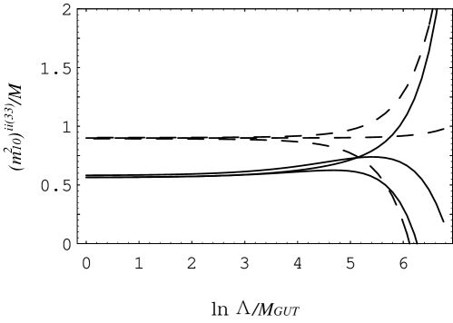
Figure 1: Converging RG flows of ${m_{10}^{2}}^{ii}/M^{2}(i=1,2)$(dashed line) and ${m_{10}^{2}}^{33}/M^{2}$(solid line).

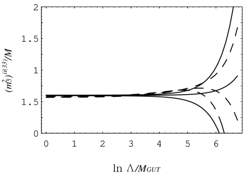
Figure 2: Converging RG flows of ${m_{5}^{2}}^{ii}/M^{2}(i=1,2)$(dashed line) and ${m_{5}^{2}}^{33}/M^{2}$(solid line).

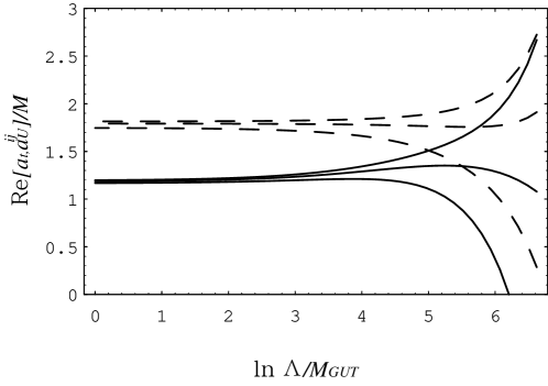
Figure 3: Converging RG flows of $\mbox{Re}[a^{ij}_{U}]/M(i,j=1,2)$(dashed line) and $\mbox{Re}[a_{t}]/M$(solid line).

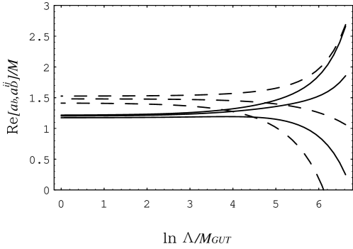
Figure 4: Converging RG flows of $\mbox{Re}[a^{ij}_{D}]/M(i,j=1,2)$(dashed line) and $\mbox{Re}[a_{b}]/M$(solid line).

It is seen that the convergence of the squared soft scalar masses are remarkable. Also the discrepances of the converging values between $(m^{2})^{ii}(i=1,2)$ and $(m^{2})^{33}$ are sizable for the 10-multiplets. The convergence of the A-parameters are weak compared with the soft scalar masses. However it will be seen that this degree of convergence gives quite enough alignment satisfying the FCNC bounds. Rather what we have to care is the sizable discrepancies between $a^{ij}(i,j=1,2)$ and $a^{33}$.

To be more explicit, we also give the converging values of SSB parameters at $M_{\rm GUT}$ in Tables 1 and 2. The range of convergence is evaluated by starting with the initial values of $m^{2}/M^{2}\in[-1,1]$ for the soft scalar masses and $a/M\in[-1,1]$ for the A-parameters at $M_{\rm PL}$. The infra-red fixed point values in the case of fixed (non-running) Yukawa couplings are also shown.

Table 1: The converging values of the squared soft scalar masses at $M_{\rm GUT}$ starting with the initial values of $m^{2}/M^{2}\in[-1,1]$ at $M_{\rm PL}$. The indeces run $i,j=1,2$. Their infra-red fixed point values in the case of fixed (non-running) Yukawa couplings are also shown.

	IR fixed points	Convergence at $M_{\rm GUT}$
$\left(m_{10}^{2}\right)^{33}/M^{2}$	0.54	0.574 $\pm$0.005
$\left(m_{5}^{2}\right)^{33}/M^{2}$	0.60	0.598 $\pm$0.002
$\left(m_{10}^{2}\right)^{ii}/M^{2}$	0.90	0.899 $\pm$0.001
$\left(m_{5}^{2}\right)^{ii}/M^{2}$	0.60	0.599 $\pm$ 0.001
$\mbox{Re}\left[\left(m_{10(5)}^{2}\right)^{ij}\right]/M^{2}$	0	0 $\pm$0.002
$\mbox{Im}\left[\left(m_{10(5)}^{2}\right)^{ij}\right]/M^{2}$	0	0 $\pm$0.002
$\mbox{Re}\left[\left(m_{10(5)}^{2}\right)^{i3}\right]/M^{2}$	0	0 $\pm 0.001(0.002)$
$\mbox{Im}\left[\left(m_{10(5)}^{2}\right)^{i3}\right]/M^{2}$	0	0 $\pm 0.001(0.002)$
$m_{h_{u}}^{2}/M^{2}$	0	0.0016 $\pm$ 0.0004
$m_{h_{d}}^{2}/M^{2}$	0	0.0012 $\pm$ 0.0008
$m_{\Sigma}^{2}/M^{2}$	1	0.9991 $\pm$ 0.0008

Table 2: The converging values of the A-parameters at $M_{\rm GUT}$ starting with the initial values of $a/M\in[-1,1]$ at $M_{\rm PL}$. The indeces run $i,j=1,2$. Their infra-red fixed point values in the case of fixed (non-running) Yukawa couplings are also shown.

	IR fixed points	Convergence at $M_{\rm GUT}$
$\mbox{Re}\left[a_{t}\right]/M$	1.12	1.18$\pm$0.01
$\mbox{Re}\left[a_{b}\right]/M$	1.26	1.17$\pm$0.01
$\mbox{Re}\left[a_{U}^{ij}\right]/M$	1.80	1.75$\pm$0.02
$\mbox{Re}\left[a_{D}^{ij}\right]/M$	1.50	1.46$\pm$0.02
$\mbox{Re}\left[a_{D}^{i3}\right]/M$	1.16	1.17$\pm$0.01
$\mbox{Im}\left[a_{t}\right]/M$	0	0$\pm$0.01
$\mbox{Im}\left[a_{b}\right]/M$	0	0$\pm$0.02
$\mbox{Im}\left[a_{U,D}^{ij}\right]/M$	0	0$\pm$0.02
$\mbox{Im}\left[a_{D}^{i3}\right]/M$	0	0$\pm$0.02
$\mbox{Re}\left[a_{f}\right]/M$	1	0.98988$\pm$0.00007

Lastly let us make some remarks on the parameters $\mu_{H}$ and $B_{H}$. It should be noted that $\mu_{H}$ receives only logarithmic corrections due to the $N=2$ supersymmetry in the bulk. On the other hand the soft parameter $B_{H}$ does not show converging behavior, since its beta function, which is given explicitly as

$$\beta(B_{H})=\left(\frac{96}{5}Mg^{2}-\frac{48}{5}a_{f}g^{2}-\frac{48}{5}a_{\bar{f}}g^{2}\right)N,$$ (40)

vanishes rapidly with scaling down. Thus we cannot explain the $\mu$ term by the RG running behavior in the extra-dimensions. However it has been known also that the $\mu$ and $B$ parameters may be generated at lower energy scale by assuming extra scalar fields hall1 ; muterm . Therefore we suppose the $\mu$ term to be generated by other mechanisms at lower energy scale and take $\mu_{H}$ and $B_{H}$ as free parameters in our analysis.

III Evaluation of FCNCs and CP violations at $M_{\rm SUSY}$

We are now interested in verifying whether the infrared attractive values of the SSB parameters given in TABLE I and II are consistent with the experimental constraints coming from the dangerous FCNC and CP-violating processes at low energies. For this purpose, first the SSB parameters should be evaluated at $M_{\rm SUSY}$. We operate the two-loop RG functions to calculate the low-energy values of the dimensionless parameters, while we use the one-loop RG functions for the SSB parameters. Then the flavor mixing masses, which are of our present concern in evaluating the amount of FCNC, are evaluated in the bases of the mass eigenstates for the quarks and leptons. To begin with, we recall that the mass matrices ${\bf M}_{I}~{}(I=u,d,e)$ for the quarks and leptons and ${\bf M}_{\nu}$ for the left-handed neutrinos, respectively, are diagonalized by the unitary matrices as

$$U_{u(d,e)L}^{{\dagger}}{\bf M}_{u(d,e)}U_{u(d,e)R} = \mbox{diag}(m_{u(d,e)},m_{c(s,\mu)},m_{t(b,\tau)}),$$ (41)

$$U_{\nu}^{T}{\bf M_{\nu}}U_{\nu} = \mbox{diag}(m_{\nu_{e}},m_{\nu_{\mu}},m_{\nu_{\tau}}).$$ (42)

These diagonalization matrices are not known, unless the matrices of Yukawa couplings are explicitly fixed. However, the mixing matrices defined by

$$V_{CKM} = U_{uL}^{{\dagger}}U_{dL}~{},~{}V_{MNS}=U_{eL}^{{\dagger}}U_{\nu},$$ (43)

are observables. Roughly $V_{\rm CKM}$ and $V_{\rm MNS}$ may be represented by the following matrices,

$$V_{\rm CKM} \sim \left(\begin{array}[]{ccc}0.98&0.22&0.003\\ -0.22&0.97&0.04\\ 0.01&-0.04&1\\ \end{array}\right)~{},~{}~{}~{}~{}V_{\rm MNS}=\left(\begin{array}[]{ccc}1/\sqrt{2}&1/\sqrt{2}&0\\ -1/2&1/2&1/\sqrt{2}\\ 1/2&-1/2&1/\sqrt{2}\\ \end{array}\right).$$ (50)

So we perform order estimation of the flavor mixing masses by simply assuming that mixings of the diagonalization matrices are similar to those of the above mixing matrices.

III.1 The slepton sector

First we consider the soft scalar masses of sleptons. The slepton mass matrices at $M_{\rm SUSY}$ are found to be

$$\frac{{\bf\tilde{m}^{2}}_{LL}}{M^{2}} = \left(\begin{array}[]{ccc}1.152\pm 0.002&0\pm 0.002(1+I)&0\pm 0.002(1+I)\\ 0\pm 0.002(1+I)&1.152\pm 0.002&0\pm 0.002(1+I)\\ 0\pm 0.002(1+I)&0\pm 0.002(1+I)&1.148\pm 0.002\end{array}\right),$$ (54)

$$\frac{{\bf\tilde{m}^{2}}_{RR}}{M^{2}} = \left(\begin{array}[]{ccc}1.054\pm 0.002&0\pm 0.002(1+I)&0\pm 0.001(1+I)\\ 0\pm 0.002(1+I)&1.054\pm 0.002&0\pm 0.001(1+I)\\ 0\pm 0.001(1+I)&0\pm 0.001(1+I)&0.718\pm 0.005\end{array}\right),$$ (58)

where $M$ denotes the gaugino mass at $M_{\rm GUT}$. Note that the branching ratios of lepton flavor violating processes are proportional to the off-diagonal elements of $U_{eL}^{\dagger}{\bf\tilde{m}^{2}}_{LL}U_{eL}$ and $U_{eR}^{\dagger}{\bf\tilde{m}^{2}}_{RR}U_{eR}$ fcnc , where the unitary matrices $U_{eL}$ and $U_{eR}$ are not explicitly known. In our following calculations, we first assume that the rotation matrices to be

$$U_{eR}\sim V_{\rm CKM}~{},~{}~{}~{}U_{eL}\sim V_{\rm MNS}^{{\dagger}},$$ (59)

which are regarded as their maximal estimations. According to fcnc , we then calculate the ratios of the off-diagonal elements of $U_{eL(R)}^{\dagger}{\bf\tilde{m}^{2}}_{LL(RR)}U_{eL(R)}$ to their diagonal elements $(m_{\tilde{l}}^{2})$, which are denoted by $(\delta^{\ell}_{ij})_{LL(RR)}$.

Here the origin of FCNC can be separated into two parts. (i)The difference of the fixed point for $({\bf\tilde{m}^{2}})^{ii}(i=1,2)$ and $({\bf\tilde{m}^{2}})^{33}$ because of $Y_{t,b}$. Note that ${\bf\tilde{m}^{2}}_{LL}$ and ${\bf\tilde{m}^{2}}_{RR}$ are embedded in the $m_{5}^{2}$ and $m_{10}^{2}$ respectively, and that the $\beta$ function of $m_{5}^{2}$ depends only on $Y_{b}$ while that of $m_{10}^{2}$ on $Y_{t}$ ((33)$\sim$(38)). Since these effects of $Y_{t,b}$ spoil the degeneracy for the soft scalar masses, the flavor mixing masses generating FCNC arise through the rotation given by Eq. (59). (ii)The deviation from the fixed points also can be the origin of FCNC. Since each parameter cannot converge exactly to the IR fixed point due to finite energy range of the GUT theory, there are small deviations from the fixed points. Therefore if we assume the initial value of parameters at $M_{\rm PL}$ to be arbitrary, then misalignment of the soft masses remains slightly and also generates FCNC.

However, it is found that ${\bf\tilde{m}^{2}}_{LL(RR)}$ given above are enough degenerate so as to suppress FCNC. While ${\bf\tilde{m}^{2}}_{RR}$ is strongly affected by $Y_{t}$ (in the meaning of (i)), the discrepancy does not give rise to a large contribution to the off-diagonal elements of $\delta_{RR}$ because of the small mixing matrix $V_{\rm CKM}$. On the other hand, the degeneracy in ${\bf\tilde{m}^{2}}_{LL}$ is good enough, even if it is transformed by the large mixing matrix $V_{\rm MNS}$ (59). This is one of our main findings on the orbifold GUT model.

Then, estimating $\delta$’s by taking into account the effects both (i) and (ii), we find:

$$\mbox{Re}\left[(\delta^{\ell}_{12})_{LL}\right] \sim 3.1\times 10^{-3}~{},~{}\mbox{Im}\left[(\delta^{\ell}_{12})_{LL}\right]\sim 2.0\times 10^{-3},$$ (60)

$$\mbox{Re}\left[(\delta^{\ell}_{13})_{LL}\right] \sim 3.8\times 10^{-3}~{},~{}\mbox{Im}\left[(\delta^{\ell}_{13})_{LL}\right]\sim 2.5\times 10^{-3}~{},$$ (61)

$$\mbox{Re}\left[(\delta^{\ell}_{23})_{LL}\right] \sim 3.8\times 10^{-3}~{},~{}\mbox{Im}\left[(\delta^{\ell}_{23})_{LL}\right]\sim 2.5\times 10^{-3},$$ (62)

$$\mbox{Re}\left[(\delta^{\ell}_{12})_{RR}\right] \sim 2.1\times 10^{-3}~{},~{}\mbox{Im}\left[(\delta^{\ell}_{12})_{RR}\right]\sim 1.5\times 10^{-3}~{},$$ (63)

$$\mbox{Re}\left[(\delta^{\ell}_{13})_{RR}\right] \sim 3.0\times 10^{-3}~{},~{}\mbox{Im}\left[(\delta^{\ell}_{13})_{RR}\right]\sim 1.3\times 10^{-3}~{},$$ (64)

$$\mbox{Re}\left[(\delta^{\ell}_{23})_{RR}\right] \sim 1.6\times 10^{-2}~{},~{}\mbox{Im}\left[(\delta^{\ell}_{23})_{RR}\right]\sim 1.3\times 10^{-3}~{}.$$ (65)

The experimental upper bounds of $(\delta^{\ell}_{ij})_{LL,RR}$ are given in fcnc , and are shown in TABLE III. Constraints appearing in TABLE III are shown in the case that the ratio of the squared photino mass and the squared slepton mass is 0.3. Actually in the case of (39),  the gaugino and the average sfermion masses are found to be

$$m_{{\tilde{q}}_{u(d)}}=3.03(3.12)M,~{}~{}m_{\tilde{l}}=1.02M,~{}~{}m_{\tilde{\gamma}}=M_{1}=0.39M,~{}~{}m_{\tilde{g}}=M_{3}=3.36M$$ (66)

at the weak scale. Therefore the ratio $m^{2}_{\tilde{\gamma}}/m^{2}_{\tilde{\ell}}$ is about $0.15$. The constraints for this case are not much different from those given in TABLE III. Here it should be noted also that the above ratios are low energy predictions for the orbifold GUT model, which are completely independent of the fundamental physics at $M_{\rm PL}$. Comparing the results given in (60)–(65) with TABLE III, it is seen that the off-diagonal elements $(\delta^{\ell}_{ij})_{LL,RR}$ are small enough to satisfy the constraints.

Table 3: Limits on the $|\delta^{\ell}_{ij}|$ from $\ell_{j}\rightarrow\ell_{i}\gamma$ decays,EDM of the electron for $m^{2}_{\tilde{\gamma}}/m^{2}_{\tilde{\ell}}=0.3$. Here the parameter $\tilde{m}_{\tilde{\ell}}$ denotes $m_{\tilde{\ell}}(\mbox{GeV})/100$. See fcnc for details.

$|(\delta^{\ell}_{12})_{LL,RR}|$	$|(\delta^{\ell}_{13})_{LL,RR}|$	$|(\delta^{\ell}_{23})_{LL,RR}|$
$4.1\times 10^{-3}~{}\tilde{m}_{\tilde{\ell}}^{2}$	$1.5\times 10^{+1}~{}\tilde{m}_{\tilde{\ell}}^{2}$	$2.8~{}\tilde{m}_{\tilde{\ell}}^{2}$
$|(\delta^{\ell}_{12})_{LR}|$	$|(\delta^{\ell}_{13})_{LR}|$	$|(\delta^{\ell}_{23})_{LR}|$
$1.4\times 10^{-6}~{}\tilde{m}_{\tilde{\ell}}^{2}$	$8.9\times 10^{-2}~{}\tilde{m}_{\tilde{\ell}}^{2}$	$1.7\times 10^{-2}~{}\tilde{m}_{\tilde{\ell}}^{2}$

To satisfy the FCNC constraints, it is also necessary to take into account the mass matrices among the left-handed and right-handed sleptons, which are generated through the A-terms . The A-parameters $a_{e}$ at the weak scale are found to be

$$\frac{a_{e}}{M}=\left(\begin{array}[]{ccc}a&a&b\\ a&a&b\\ b&b&c\end{array}\right),~{}~{}~{}\begin{array}[]{l}a=(2.175\pm 0.023)+I~{}(0\pm 0.023)\\ b=c=(1.888\pm 0.014)+I~{}(0\pm 0.018).\end{array}$$ (72)

The left-right mixing mass matrix is given by ${\bf\tilde{m}^{2}}_{LR}=v_{d}h_{e}=-v_{d}(Y_{e}a_{e})$, where

$$v_{d}Y_{e}=U_{eL}~{}m_{e}^{diag}~{}U_{eR}^{{\dagger}}=\left(\begin{array}[]{ccc}-6.9&-12.1&890.0\\ 7.7&11.9&-890.0\\ 22.9&128.6&1252.0\end{array}\right)~{}(\mbox{MeV}).$$ (76)

There are two origins of FCNC here again, that is, (i)the flavor non-universality in the fixed points due to the Yukawa couplings. It spoils the alignment of the A-term. (ii)The deviations from the fixed point values similar to the case of the scalar masses. This effect is actually irrelevant for the left-right mixing masses. Now the index $(\delta^{\ell})_{LR}$ is given by the ratio of ${\bf\tilde{m}^{2}}_{LR}$ and the average slepton mass squared $m^{2}_{\tilde{\ell}}$. Note that the left-right mixing mass matrix is given by the product of the A-parameters proportional to the gaugino mass scale and the lepton mass matrix (76), which does not depend on the gaugino mass. Therefore, $\delta_{LR}$ is dependent on the SSB mass scale differently from $\delta_{LL(RR)}$. Here we represent the index in the unit of $100{\mbox{GeV}}$ for the slepton mass. Then $(\delta^{\ell})_{LR}$ are estimated as follows,

$$\mbox{Re}[(\delta^{\ell}_{12})_{LR}] \sim 1.3\times 10^{-4}\left(\frac{100}{m_{\tilde{\ell}}(\mbox{GeV})}\right)^{2},~{}$$ (77)

$$\mbox{Re}[(\delta^{\ell}_{13})_{LR}] \sim 1.3\times 10^{-4}\left(\frac{100}{m_{\tilde{\ell}}(\mbox{GeV})}\right)^{2},~{}$$ (78)

$$\mbox{Re}[(\delta^{\ell}_{23})_{LR}] \sim 3.8\times 10^{-4}\left(\frac{100}{m_{\tilde{\ell}}(\mbox{GeV})}\right)^{2}.$$ (79)

All the fixed points are real and, therefore, the imaginary parts of the left-right mixings can be treated as zero.

Unfortunately $(\delta^{\ell}_{12})_{LR}$ obtained in this analysis exceeds the experimental bound given in TABLE III. This is due to the large mixings of the $V_{\rm MNS}$ matrix. However, this implies only that our assumption $U_{eL}=V_{\rm MNS}$, which would be maximal estimation of the matrix, is not viable phenomenologically in the orbifold GUT models. Therefore let us repeat the above estimation by setting $U_{eL}=V_{\rm CKM}$, for example. Then it is found that the indices $(\delta_{ij})_{LR}$ become fairly smaller, such as

$$\mbox{Re}[(\delta^{\ell}_{12})_{LR}] \sim 1.1\times 10^{-5}\left(\frac{100}{m_{\tilde{\ell}}(\mbox{GeV})}\right)^{2}.$$ (80)

This result shows that the BRs of dangerous lepton flavor violating processes like $\mu\to e+\gamma$ do not exceed the stringent bounds as long as $m_{\tilde{\ell}}>170{\mbox{GeV}}$. As results of the above analyses, it may be said that the lepton flavor violation as well as the CP violation can be less than their present experimental bounds, in the case of $U_{eL}$ containing only small mixings.

III.2 The squark sector

As in the leptonic sector (58), the squark soft mass matrices turn out at $M_{\rm SUSY}$ to be

$$\frac{{\bf\tilde{m}^{2}}_{QLL}}{M^{2}} = \left(\begin{array}[]{ccc}10.542\pm 0.002&0\pm 0.002(1+I)&0\pm 0.001(1+I)\\ 0\pm 0.002(1+I)&10.542\pm 0.002&0\pm 0.001(1+I)\\ 0\pm 0.001(1+I)&0\pm 0.001(1+I)&8.192\pm 0.002\end{array}\right),$$ (84)

$$\frac{{\bf\tilde{m}^{2}}_{uRR}}{M^{2}} = \left(\begin{array}[]{ccc}10.092\pm 0.002&0\pm 0.002(1+I)&0\pm 0.001(1+I)\\ 0\pm 0.002(1+I)&10.092\pm 0.002&0\pm 0.001(1+I)\\ 0\pm 0.001(1+I)&0\pm 0.001(1+I)&5.7878\pm 0.002\end{array}\right),$$ (88)

$$\frac{{\bf\tilde{m}^{2}}_{dRR}}{M^{2}} = \left(\begin{array}[]{ccc}9.741\pm 0.002&0\pm 0.002(1+I)&0\pm 0.001(1+I)\\ 0\pm 0.002(1+I)&9.741\pm 0.002&0\pm 0.001(1+I)\\ 0\pm 0.001(1+I)&0\pm 0.001(1+I)&9.678\pm 0.001\end{array}\right).$$ (92)

We can obtain $\delta$’s by estimating $U_{uL(uR)}^{{\dagger}}{\bf\tilde{m}^{2}}_{QLL(uRR)}U_{uL(uR)}$ and $U_{dL(dR)}^{{\dagger}}{\bf\tilde{m}^{2}}_{QLL(dRR)}U_{dL(dR)}$. Also here we assume that

$$U_{uR}=U_{uL}=U_{dL}=V_{\rm CKM}~{},~{}U_{dR}=V_{\rm MNS}^{{\dagger}},$$ (93)

therefore $(\delta^{u})_{LL}=(\delta^{d})_{LL}$.

Taking into account the FCNC contribution from both (i) and (ii), we find that

$$\mbox{Re}[(\delta^{u,d}_{12})_{LL}] \sim 2.6\times 10^{-4}~{},~{}\mbox{Im}[(\delta^{u,d}_{12})_{LL}]\sim 1.6\times 10^{-4}~{},$$ (94)

$$\mbox{Re}[(\delta^{u,d}_{13})_{LL}] \sim 1.3\times 10^{-3}~{},~{}\mbox{Im}[(\delta^{u,d}_{13})_{LL}]\sim 1.2\times 10^{-4}~{},$$ (95)

$$\mbox{Re}[(\delta^{u,d}_{23})_{LL}] \sim 1.1\times 10^{-2}~{},~{}\mbox{Im}[(\delta^{u,d}_{23})_{LL}]\sim 1.2\times 10^{-4}~{},$$ (96)

$$\mbox{Re}\left[(\delta^{u}_{12})_{RR}\right] \sim 3.5\times 10^{-4}~{},~{}\mbox{Im}\left[(\delta^{u}_{12})_{RR}\right]\sim 1.8\times 10^{-4}~{},$$ (97)

$$\mbox{Re}\left[(\delta^{u}_{13})_{RR}\right] \sim 2.6\times 10^{-3}~{},~{}\mbox{Im}\left[(\delta^{u}_{13})_{RR}\right]\sim 1.2\times 10^{-4}~{},$$ (98)

$$\mbox{Re}\left[(\delta^{u}_{23})_{RR}\right] \sim 2.2\times 10^{-2}~{},~{}\mbox{Im}\left[(\delta^{u}_{23})_{RR}\right]\sim 1.1\times 10^{-4}~{},$$ (99)

$$\mbox{Re}\left[(\delta^{d}_{12})_{RR}\right] \sim 1.9\times 10^{-3}~{},~{}\mbox{Im}\left[(\delta^{d}_{12})_{RR}\right]\sim 2.2\times 10^{-4}~{},$$ (100)

$$\mbox{Re}\left[(\delta^{d}_{13})_{RR}\right] \sim 2.6\times 10^{-3}~{},~{}\mbox{Im}\left[(\delta^{d}_{13})_{RR}\right]\sim 2.6\times 10^{-4}~{},$$ (101)

$$\mbox{Re}\left[(\delta^{d}_{23})_{RR}\right] \sim 2.6\times 10^{-3}~{},~{}\mbox{Im}\left[(\delta^{d}_{23})_{RR}\right]\sim 2.6\times 10^{-4}~{}.$$ (102)

The upper bounds for $\delta$’s coming from the measurements of $K-\bar{K}$, $D-\bar{D}$, $B_{d}-\bar{B}_{d}$ mixing, $\epsilon_{K}$, $b\rightarrow s~{}\gamma$ and $\epsilon^{\prime}/\epsilon$ fcnc are shown in TABLE IV, where the imaginary parts are constrained by CP-violating processes. It is seen that $\delta$’s given above satisfy well the experimental constraints except for $\sqrt{|\mbox{Im}(\delta^{d}_{12})_{LL}(\delta^{d}_{12})_{RR}|}$, which is comparable to the constraint.

Table 4: Limits on the $|\delta^{d(u)}_{ij}|$ from $K-\bar{K}$, $D-\bar{D}$, $B_{d}-\bar{B}_{d}$ mixing, $\epsilon_{K}$, $b\rightarrow s~{}\gamma$ and $\epsilon^{\prime}/\epsilon$ for $m_{\tilde{g}}^{2}/m_{\tilde{q}}^{2}=1$ fcnc . Here the parameter $\tilde{m}_{\tilde{q}}$ denotes $m_{\tilde{q}}(\mbox{GeV})/500$.

$\sqrt{|\mbox{Re}(\delta^{d}_{12})^{2}_{LL,RR}|}$	$\sqrt{|\mbox{Re}(\delta^{d}_{12})_{LL}(\delta^{d}_{12})_{RR}|}$	$\sqrt{|\mbox{Re}(\delta^{d}_{12})^{2}_{LR}|}$
$4.0\times 10^{-2}~{}\tilde{m}_{\tilde{q}}$	$2.8\times 10^{-3}~{}\tilde{m}_{\tilde{q}}$	$4.4\times 10^{-3}~{}\tilde{m}_{\tilde{q}}$
$\sqrt{|\mbox{Re}(\delta^{d}_{13})^{2}_{LL,RR}|}$	$\sqrt{|\mbox{Re}(\delta^{d}_{13})_{LL}(\delta^{d}_{13})_{RR}|}$	$\sqrt{|\mbox{Re}(\delta^{d}_{13})^{2}_{LR}|}$
$9.8\times 10^{-2}~{}\tilde{m}_{\tilde{q}}$	$1.8\times 10^{-2}~{}\tilde{m}_{\tilde{q}}$	$3.3\times 10^{-3}~{}\tilde{m}_{\tilde{q}}$
$\sqrt{|\mbox{Re}(\delta^{u}_{12})^{2}_{LL,RR}|}$	$\sqrt{|\mbox{Re}(\delta^{u}_{12})_{LL}(\delta^{u}_{12})_{RR}|}$	$\sqrt{|\mbox{Re}(\delta^{u}_{12})^{2}_{LR}|}$
$1.0\times 10^{-1}~{}\tilde{m}_{\tilde{q}}$	$1.7\times 10^{-2}~{}\tilde{m}_{\tilde{q}}$	$3.1\times 10^{-3}~{}\tilde{m}_{\tilde{q}}$
$\sqrt{|\mbox{Im}(\delta^{d}_{12})^{2}_{LL,RR}|}$	$\sqrt{|\mbox{Im}(\delta^{d}_{12})_{LL}(\delta^{d}_{12})_{RR}|}$	$\sqrt{|\mbox{Im}(\delta^{d}_{12})^{2}_{LR}|}$
$3.2\times 10^{-3}~{}\tilde{m}_{\tilde{q}}$	$2.2\times 10^{-4}~{}\tilde{m}_{\tilde{q}}$	$3.5\times 10^{-4}~{}\tilde{m}_{\tilde{q}}$
$|(\delta^{d}_{23})_{LL,RR}|$		$|(\delta^{d}_{23})_{LR}|$
$8.2~{}\tilde{m}_{\tilde{q}}^{2}$		$1.6\times 10^{-2}~{}\tilde{m}_{\tilde{q}}^{2}$
$|\mbox{Im}(\delta^{d}_{12})_{LL,RR}|$		$|\mbox{Im}(\delta^{d}_{12})_{LR}|$
$4.8\times 10^{-1}~{}\tilde{m}_{\tilde{q}}^{2}$		$2.0\times 10^{-5}~{}\tilde{m}_{\tilde{q}}^{2}$

The mixing masses between the left-handed and right-handed squarks and also their effects to FCNC and CP-violation may be evaluated just as done for the slepton sector. The A-parameters at the weak scale are given by

$$\frac{a_{u}}{M} = \left(\begin{array}[]{ccc}a&a&b\\ a&a&b\\ b&b&c\end{array}\right),~{}~{}~{}\begin{array}[]{l}a=(4.929\pm 0.020)+I~{}(0\pm 0.017)\\ b=(2.701\pm 0.007)+I~{}(0\pm 0.005)\\ c=(2.705\pm 0.001)+I~{}(0\pm 0.002),\\ \end{array}$$ (109)

$$\frac{a_{d}}{M} = \left(\begin{array}[]{ccc}a&a&b\\ a&a&b\\ b&b&c\end{array}\right),~{}~{}~{}\begin{array}[]{l}a=(6.241\pm 0.020)+I~{}(0\pm 0.017)\\ b=c=(5.391\pm 0.013)+I~{}(0\pm 0.016),\end{array}$$ (115)

The indices $\delta$, which should be compared with the experimental constraints shown also in TABLE IV, are found to be

$$\mbox{Re}\left[(\delta^{u}_{12})_{LR}\right] \sim 3.9\times 10^{-4}~{}\tilde{m}_{\tilde{q_{u}}}^{-2}~{},~{}\mbox{Im}\left[(\delta^{u}_{12})_{LR}\right]\sim 4.1\times 10^{-5}~{}\tilde{m}_{\tilde{q}_{u}}^{-2}~{},$$ (116)

$$\mbox{Re}\left[(\delta^{u}_{13})_{LR}\right] \sim 7.7\times 10^{-5}~{}\tilde{m}_{\tilde{q}_{u}}^{-2}~{},~{}\mbox{Im}\left[(\delta^{u}_{13})_{LR}\right]\sim 6.2\times 10^{-5}~{}\tilde{m}_{\tilde{q}_{u}}^{-2}~{},$$ (117)

$$\mbox{Re}\left[(\delta^{u}_{23})_{LR}\right] \sim 6.5\times 10^{-4}~{}\tilde{m}_{\tilde{q}_{u}}^{-2}~{},~{}\mbox{Im}\left[(\delta^{u}_{23})_{LR}\right]\sim 2.3\times 10^{-4}~{}\tilde{m}_{\tilde{q}_{u}}^{-2}~{},$$ (118)

$$\mbox{Re}\left[(\delta^{d}_{12})_{LR}\right] \sim 3.9\times 10^{-5}~{}\tilde{m}_{\tilde{q}_{d}}^{-2}~{},~{}\mbox{Im}\left[(\delta^{d}_{12})_{LR}\right]\sim 1.4\times 10^{-5}~{}\tilde{m}_{\tilde{q}_{d}}^{-2}~{},$$ (119)

$$\mbox{Re}\left[(\delta^{d}_{13})_{LR}\right] \sim 1.5\times 10^{-4}~{}\tilde{m}_{\tilde{q}_{d}}^{-2}~{},~{}\mbox{Im}\left[(\delta^{d}_{13})_{LR}\right]\sim 1.8\times 10^{-4}~{}\tilde{m}_{\tilde{q}_{d}}^{-2}~{},$$ (120)

$$\mbox{Re}\left[(\delta^{d}_{23})_{LR}\right] \sim 2.2\times 10^{-4}~{}\tilde{m}_{\tilde{q}_{d}}^{-2}~{},~{}\mbox{Im}\left[(\delta^{d}_{23})_{LR}\right]\sim 2.6\times 10^{-4}~{}\tilde{m}_{\tilde{q}_{d}}^{-2}~{},$$ (121)

where $\tilde{m}_{\tilde{q}_{u(d)}}^{-2}=(500/m_{\tilde{q}_{u(d)}}(\mbox{GeV}))^{2}$. For squarks, all of them are small enough to suppress the FCNC and the CP violation within the bounds, although we have assumed $U_{dR}$ to be the bi-maximal mixing matrix.

IV Conclusion

In this paper, we investigated how much the infra-red attractive force of gauge interactions can soften the SUSY flavor problem in the orbifold GUT of Kawamura kawamura1 . First we discussed the notion of gauge coupling unification in the orbifold GUT models, where the unified gauge symmetry is explicitly broken by the boundary conditions. It is natural for the bulk theory to recover the unified symmetry as the scale goes much shorter than the radius of compactified dimensions. We showed explicitly that the running gauge couplings defined in the extra-dimensional sense approach to each other asymptotically (asymptotic unification). In the four-dimensional picture, this occurs due to the power-law running behavior of the gauge couplings.

The radiative corrections by the bulk gauge fields make the SSB parameters subject to the power-law running also. Then the ratio of the SSB parameters to the gaugino mass at the compactification scale are fixed to their infra-red attractive fixed point values, which are totally flavor universal kubo6 . It should be noted that the SSB parameters at low energy are also fixed solely by the gaugino mass scale, and, therefore, insensitive to those in the fundamental theory. Thus this suggests an interesting possibility for the SUSY flavor problem and the CP problem.

We examined the one-loop RG flows for the general soft SSB parameters in the orbifold GUT models. Then the Yukawa couplings to the bulk Higgs fields, which also show power-law running behavior, split the SSB parameters of the first two and the third generations. In the calculations we neglected the logarithmic corrections including the breaking effects of the GUT symmetry due to boundary conditions, since the most dominant flavor dependence comes from the corrections due to the bulk Yukawa couplings. We assumed also $M_{\rm PL}/M_{c}\sim 10^{3}$.

Now there are two sources for the flavor violating masses of the SUSY particles; (i) flavor dependence in the fixed points induced by the Yukawa couplings, (ii) deviation from the fixed point values due to finite radius of the compactified dimensions. As for (ii), we found that the arbitrary disorder in the SSB parameters at the fundamental scale are sufficiently suppressed at $M_{\rm GUT}$. Therefore this effect does not cause any problems in FCNC processes or in dangerous CP-violating phenomena, since the fixed points are real. So what we should be concerned more is the effect (i) in the orbifold GUT models.

The key ingredients for the FCNC processes are the flavor changing elements of the mass matrices of squarks and sleptons obtained after rotation to the basis of mass eigenstates for quarks and leptons. However the rotation matrices are unknown, though the mixing matrices $V_{\rm CKM}$ and $V_{\rm NMS}$ are given experimentally. We first assume that the rotation matrices of the fields belonging to ${\bf 10}$ of SU(5) GUT are given by $V_{\rm CKM}$, while the rotation matrices of the fields belonging to $\overline{\bf 5}$ are $V_{\rm NMS}$ (59). This would be regarded as the maximal estimation of the rotations. Then it is found that the indices of the off-diagonal elements of the soft scalar masses $\delta_{LL}$ and $\delta_{RR}$ are both suppressed sufficiently. The reason of this is as follows. Indeed splitting of the fixed points values for the third generation to others are sizable for the fields in ${\bf 10}$ due to large $Y_{t}$. However the rotation matrix $V_{\rm CKM}$ contains only small mixings. On the other hand the degeneracy of the fixed points for the fields in $\overline{\bf 5}$ is fairly good. Therefore the off-diagonal elements remain tiny, even if the mass matrices are transformed by the large mixing matrix $V_{\rm MNS}$.

Unfortunately, however, it is found to be hard for the A-parameters to satisfy the experimental constraints under the above assumption on the rotation matrices. The index $(\delta^{\ell}_{12})_{LR}$ in the slepton sector appears exceeding the present experimental bound, though all the other indices in the both sectors are lower than their limit. However, if the rotation matrix $U_{eL}$ is a small mixing one like $V_{\rm CKM}$, (namely $V_{\rm MNS}\sim U_{\nu}$), then the index $(\delta^{\ell}_{12})_{LR}$ is found to become lower than the constraint unless the slepton masses are very light. Thus our mechanism can soften the SUSY flavor problem and also the CP problem. After all we conclude that the mechanism of kubo6 to solve the SUSY flavor problem may be combined with the mechanism of kawamura1 to overcome the doublet-triplet splitting problem in extra dimensions.

In this paper we have not discussed the case with the right-handed neutrino. It has been well-known that the Yukawa coupling between the lepton-doublet and the right-handed neutrino generates sizable mixings in the slepton masses in comparison with the current bounds for the lepton violating processes bm ; LFV , unless the neutrino Yukawa coupling is rather small. This effect is caused by the large mixing angles of $V_{\rm MNS}$. In the orbifold GUT, the fixed points are not degenerate, therefore the off-diagonal elements would be generated more due to the large mixings. Also it should be concerned also that the running above the GUT scale is affected by the neutrino Yukawa coupling GUTmixing . Then larger mass mixings could appear in $\bar{\bf 5}$-sector, therefore not only the sleptons but also the squarks sectors should be reanalyzed. Here we would like to leave these problems to future studies.

References

• (1) For a recent review, see, for instance, G. L. Kane, hep-ph/0202185, and references therein.
• (2) S. Weinberg, Phys. Rev. D26, 287 (1982); N. Sakai and T. Yanagida, Nucl. Phys. B197, 533 (1982).
• (3) H. Murayama and A. Pierce, Phys. Rev. D65, 055009 (2002).
• (4) Y. Kawamura, Prog. Theor. Phys. 105, 691 (2001); 105, 999 (2001).
• (5) R. Barbieri, L.J. Hall and Y. Nomura, Phys. Rev. D63, 105007 (2001).
• (6) G. Altarelli and F. Feruglio, Phys. Lett. B511, 257 (2001).
• (7) L.J. Hall and Y. Nomura, Phys. Rev. D64, 055003 (2001).
• (8) E. Witten, hep-ph/0201018; T. Friedmann and E. Witten, hep-th/0211269.
• (9) S. Dimopoulos and D. Sutter, Nucl. Phys. B452, 496 (1995).
• (10) L. Hall, V.A. Kostelecky and S. Raby, Nucl. Phys. B267, 415 (1986); F. Gabbiani and A. Masiero, Phys. Lett. B209, 289 (1988).
• (11) J. Ellis and D.V. Nanopoulos, Phys. Lett. B110, 44 (1982); R. Barbieri and R. Gatto, Phys. Lett. B110, 211 (1982); B. Campbell, Phys. Rev. D 28, 209 (1983); M.J. Duncan, Nucl. Phys. B221, 285 (1983); J.F. Donoghue and H.P. Nilles and D. Wyler, Phys. Lett. B128, 55 (1983).
• (12) J. Ellis, S. Ferrara and D.V. Nanopoulos, Phys. Lett. B114, 231 (1982); W. Buchmüller and D. Wyler, Phys. Lett. B121, 321 (1983); J. Polchinski and M.B. Wise, Phys. Lett. B125, 393 (1983); F. del Aguila, M.B. Gavela, J.A. Grifols and A. Méndez, Phys. Lett. B126, 71 (1983); D.V. Nanopoulos and M. Srednicki, Phys. Lett. B128, 61 (1983).
• (13) S. Bertolini, F. Borzumati, A. Masiero and G. Ridolfi, Nucl. Phys. B353, 591 (1991); R. Barbieri and G.F. Giudice, Phys. Lett. B309, 86 (1993).
• (14) F. Gabbiani, E. Gabrielli, A. Masiero and L. Silvestrini, Nucl. Phys. B477, 321 (1996); A. Bartl, T. Gajdosik, E. Lunghi, A. Masiero, W. Porod, H. Stremnitzer and O. Vives, Phys. Rev. D64, 076009 (2001), and references therein.
• (15) M. Dine and A. E. Nelson, Phys. Rev. D48, 1277 (1993); M. Dine, A. E. Nelson and Y. Shirman, Phys. Rev. D51, 1362 (1995); For a review, G. F. Giudice and R. Rattazzi, Phys. Rept. 322, 419 (1999).
• (16) L. Randall and R. Sundrum, Nucl. Phys. B557, 79 (1999); G. F. Giudice, M. A. Luty, H. Murayama and R. Rattazi, JHEP 12, 027 (1998).
• (17) D. E. Kaplan, G. D. Kribs and M. Schmaltz, Phys. Rev. D62, 035010 (2000); Z. Chacko, M. A. Luty, A. E. Nelson and E. Ponton, JHEP 01, 003 (2000).
• (18) L.J. Hall and H. Murayama, Phys. Rev. Lett. 75 (1995) 3985; C.D. Carone, L.J. Hall and H. Murayama, Phys. Rev. D53, 6282 (1996).
• (19) K. Hamaguchi, M. Kakizaki and M. Yamaguchi, Phys. Rev. D68, 056007 (2003).
• (20) K.S. Babu, T. Kobayashi and J. Kubo, Phys. Rev. D67, 075018 (2003).
• (21) T. Kobayashi, J. Kubo and H. Terao, Phys. Lett. B568, 83 (2003).
• (22) M. Lanzagorta and G.G. Ross, Phys. Lett. B364, 163 (1995); P.M. Ferreira, I. Jack and D.R.T. Jones, Phys. Lett. B357, 359 (1995); S.A. Abel and B.C. Allanach, Phys. Lett. B415, 371 (1997); S.F. King and G.G. Ross, Nucl. Phys. B530, 3 (1998); I. Jack and D.R.T. Jones, Phys. Lett. B443, 177 (1998); G.K. Yeghiyan, M. Jurcisin and D.I. Kazakov, Mod. Phys. Lett. A14, 601 (1999); M. Jurcisin and D.I. Kazakov, Mod. Phys. Lett. A14, 671 (1999).
• (23) A. Karch, T. Kobayashi, J. Kubo, and G. Zoupanos, Phys. Lett. B441, 235 (1998); M. Luty and R. Rattazzi, JHEP 11, 001 (1999).
• (24) A. E. Nelson and M. J. Strassler, JHEP 09, (2000) 030; T. Kobayashi and H. Terao, Phys. Rev. D64, 075003 (2001).
• (25) T. Kobayashi , H. Nakano and H. Terao, Phys. Rev. D65, 015006 (2002); T. Kobayashi, H. Nakano, T. Noguchi and H. Terao, Phys. Rev. D66 095011 (2002); JHEP 0302, 022 (2003).
• (26) M. A. Luty and R. Sundrum, Phys. Rev. D65, 066004 (2002); Phys. Rev. D67, 045007 (2003).
• (27) S.A. Abel and S.F. King, Phys. Rev. D59, 095010 (1999); T. Kobayashi and K. Yoshioka, Phys. Rev. D62, 115003 (2000); M. Bando, T. Kobayashi, T. Noguchi and K. Yoshioka, Phys. Rev. D63, 113017 (2001).
• (28) J. Kubo and H. Terao, Phys. Rev. D66, 116003 (2002).
• (29) K-S. Choi, K-Y. Choi and J.E. Kim, Phys. Rev. D68, 035003 (2003).
• (30) K-Y. Choi, J.E. Kim and H. M. Lee, JHEP 0306, 040 (2003).
• (31) T. R. Taylor and G. Veneziano, Phys. Lett. B212, 147 (1988).
• (32) K. Dienes, E. Dudas and T. Gherghetta, Nucl. Phys. B537, 47 (1999).
• (33) T. Kobayashi, J. Kubo, M. Mondragon and G. Zoupanos, Nucl. Phys. B550, 99 (1999).
• (34) S. Ejiri, J. Kubo and M. Murata, Phys. Rev. D62, 105025 (2000).
• (35) R. Barbieri and L. J. Hall, Phys. Lett. B338 (1994) 212; R. Barbieri, L. J. Hall and A. Strumia, Nucl. Phys. B445 (1995) 219; B449 (1995) 437; P. Ciafaloni, A. Romanino and A. Strumia, Nucl. Phys. B458 (1996) 3; J. Hisano, T. Moroi, K. Tobe and M. Yamaguchi, Phys. Lett. B391 (1997) 341; J. Hisano, D. Nomura, Y. Okada, Y.Shimizu and M. Tanaka, Phys. Rev. D58 (1998) 116010; J. Hisano, D. Nomura and T. Yanagida, Phys. Lett. B437 (1998) 351.
• (36) J. Kubo, H. Terao and G. Zoupanos, Nucl. Phys. B574, 495 (2000).
• (37) K. Dienes, E. Dudas and T. Gherghetta, Phys. Rev. Lett. 91, 061601 (2003).
• (38) I. Antoniadis, Phys. Lett. B246, 377 (1990); I. Antoniadis, C. Muñoz and M. Quirós, Nucl. Phys. B397, 515 (1993).
• (39) N. Arkani-Hamed, S. Dimopoulos and G. Dvali, Phys. Rev. D59, 086004 (1999).
• (40) G.F. Giudice and A. Masireo, Phys. Lett. B206, 480 (1988).
• (41) A. Anisimov, M. Dine, M. Graesser and S. Thomas, Phys. Rev. D65 (2002) 105011; JHEP 0203 (2002) 036.
• (42) A. Hebecker and J. March-Russell, Phys. Lett. B539 (2002) 119.
• (43) L. J. Hall, Y. Nomura and A. Pierce, Phys. Lett. B538 (2002) 359.
• (44) F. Borzumati and A. Masiero, Phys. Rev. Lett. 57 (1986) 961.
• (45) J. Hisano, T. Moroi, K. Tobe, M. Yamaguchi and T. Yanagida, Phys. Lett. B357 (1995) 579; J. Hisano, T. Moroi, K. Tobe and M. Yamaguchi, Phys. Rev. D53 (1996) 2442; J. Hisano and D. Nomura, Phys. Rev. D59 (1999) 116005; W. Buchmüller, D. Delepine and F. Vissani, Phys. Lett. B459 (1999) 171; M. E. Gomez, G. K. Leontaris, S. Lola and J. D. Vergados, Phys. Rev. D59 (1999) 116009; J. R. Ellis, M. E. Gomez, G. K. Leontaris, S. Lola and D. V. Nanopoulos, Eur. Phys. J. C. 14 (2000) 319; W. Buchmüller, D. Delepine and L. T. Handoko, Nucl. Phys. B576 (2000) 445; J. L. Feng, Y. Nir and Y. Shadmi, Phys. Rev. D61 (2000) 113005; J. Sato, K. Tobe and T. Yanagida, Phys. Lett. B498 (2001) 189; J. Sato, K. Tobe, Phys. Rev. D63 (2001) 116010; S. Lavignac, I. Masina and C. A. Savoy, Nucl. Phys. B633 (2002) 139.
• (46) T. Moroi, JHEP 0003 (2000) 019; Phys. Lett. B493 (2000) 366; N. Akama, Y. Kiyo, S. Komine and T. Moroi, Phys. Rev. D64 (2001) 095012; S. W. Baek, T. Goto, Y. Okada and K. i. Okumura, Phys. Rev. D63 (2001) 051701; T. Goto, Y. Okada, Y. Shimizu, T. Shindou and M. Tanaka, Phys. Rev. D66 (2002) 035009; D. Chang, A. Masiero and H. Murayama, Phys. Rev. D67 (2003) 075013; J. Hisano and Y. Shimizu, Phys. Lett. B565 (2003) 183.