We calculate the amplitudes and the cross sections of the charm dissociation processes $J/\psi+\pi\to D\overline{D},D^{\ast}\overline{D}\,(\overline{D^{\ast}}D),D^{\ast}\overline{D^{\ast}}$ within a relativistic constituent quark model. We consistently account for the contributions coming from both the box and triangle diagrams that contribute to the dissociation processes. The cross section is dominated by the $D^{\ast}\overline{D}$ and $D^{\ast}\overline{D^{\ast}}$ channels. When summing up the four channels we find a maximum total cross section of about 2.3 mb at $\sqrt{s}\approx 4.1$ GeV. We compare our results to the results of other model calculations.

$J/\psi$ dissociation cross sections in a relativistic quark model

I Introduction

The analysis of the $J/\psi$ dissociation cross section is important for understanding the suppression of $J/\psi$ production observed in Pb-Pb collisions by the NA50 Collaboration at the CERN Super Proton Synchrotron (SPS) NA50 . There are a number of theoretical calculations on the $c\bar{c}$ + light hadron cross sections (see, e.g., the review Ref. Barnes:2003vt ). However, they give widely divergent results, which implies that one is still far away from a real understanding of the scattering mechanism. The nonrelativistic quark model has been applied in Martins:1994hd and Wong:1999zb ; Wong:2001td ; Barnes:2003dg for the calculation of the cross sections for the dissociation processes $c\bar{c}+q\bar{q}\to c\bar{q}+q\bar{c}$. The calculated cross sections for the reactions $J/\psi+\pi\to D\overline{D}$, $D^{\ast}\overline{D}$, $D\overline{D^{\ast}}$, $D^{\ast}\overline{D^{\ast}}$ have the following common features: they rise very fast from zero at threshold to a maximum value and finally fall off due the Gaussian form of the potential. The magnitude of the maximum total cross section was found to be $\approx 7$ mb at $\sqrt{s}\approx 4.1$ GeV in Martins:1994hd and a somewhat smaller value of $\approx 1.4$ mb at $\sqrt{s}\approx 3.9$ GeV in Wong:1999zb ; Wong:2001td ; Barnes:2003dg .

Another approach to studying the charm dissociation process started with the model proposed by Matinian and Müller Matinian:1998cb . They assumed that the dissociation cross section is dominated, in the $t$ channel, by the D meson exchange. A generalization of this approach can be found in Haglin:1999xs ; Haglin:2003fh ; Lin:1999ad ; Oh:2000qr ; Oh:2002vg ; Ivanov:2001th where an effective chiral SU(4) Lagrangian was employed. Such an approach seems to us quite problematic for the following reasons: (i) SU(4) is a badly broken symmetry, and (ii) some of the couplings in the chiral SU(4) Lagrangian are unknown. Nevertheless, this is a relativistic approach that allows one to study the above processes in a systematic fashion. In this framework, the dissociation cross section of $J/\psi$ by light hadrons is predicted to be, near the physical threshold, in the range 1-10 mb. Moreover, it is interesting to refer to the paper Oh:2002vg , where the $J/\psi$ dissociation by $\pi$ and $\rho$ mesons was examined in the meson exchange model Oh:2002vg and compared to the quark interchange model. The authors of this paper found that the meson exchange model could give predictions similar to those of the quark interchange models, not only for the magnitudes but also for the energy dependence of the low-energy dissociation cross sections of the $J/\psi$ by $\pi$ and $\rho$ mesons.

It appears that the microscopic quark nature of hadrons is important in the charm dissociation processes. The first step is to calculate the relevant form factors corresponding to the triple and quartic meson vertices in the kinematical region of the dissociation reaction. QCD sum rules have been used in Refs.  Navarra:2001jy ; Navarra:2001ju ; Matheus:2002nq ; Duraes:2002ux to evaluate those form factors and to determine the charm cross section. The cross section was found to be about 1 mb at $\sqrt{s}\approx 4.1$ GeV with a monotonic growth when the energy is increased Duraes:2002ux .

An approach based on the 1/N expansion in QCD combined with the Regge theory gives, for the total dissociation cross section, a value of a few millibarns near to $\sqrt{s}\approx 4$ GeV 1/N_Regge .

We also mention the work of Deandrea et al., where the strong couplings $J/\psi D^{\ast}D^{\ast}$ and $J/\psi D^{\ast}D^{\ast}\pi$ were evaluated in the constituent quark model Deandrea:2003pv . Finally, an extension of the finite-temperature Dyson-Schwinger equation approach to heavy mesons and its application to the reaction $J/\psi+\pi\to D+\overline{D}$ was considered in Blaschke:2000zm .

We employ a relativistic quark model model-1 to calculate the charm dissociation amplitudes and cross sections. This model is based on an effective Lagrangian which describes the coupling of hadrons $H$ to their constituent quarks. The coupling strength is determined by the compositeness condition $Z_{H}=0$ z=0 where $Z_{H}$ is the wave function renormalization constant of the hadron $H$. One starts with an effective Lagrangian written down in terms of quark and hadron fields. Then, by using Feynman rules, the S-matrix elements describing the hadronic interactions are given in terms of a set of quark diagrams. In particular, the compositeness condition enables one to avoid a double counting of the hadronic degrees of freedom. The approach is self-consistent and universally applicable. All calculations of physical observables are straightforward. The model has only a small set of adjustable parameters given by the values of the constituent quark masses and the scale parameters that define the size of the distribution of the constituent quarks inside a given hadron. The values of all fit parameters are within the window of expectations.

The shape of the vertex functions and the quark propagators can in principle be found from an analysis of the Bethe-Salpeter and Dyson-Schwinger equations as was done, e.g., in Ivanov:1998ms . In this paper, however, we choose a phenomenological approach where the vertex functions are modeled by a Gaussian form, the size parameter of which is determined by a fit to the leptonic and radiative decays of the lowest-lying light, charm, and bottom mesons. For the quark propagators we use a local representation.

We calculate the amplitudes and the cross sections of the charm dissociation processes

$$J/\psi+\pi \to D+\overline{D},$$

$$J/\psi+\pi \to D^{\ast}+\overline{D}\,\,\,(\overline{D^{\ast}}+D),$$

$$J/\psi+\pi \to D^{\ast}+\overline{D^{\ast}}.$$

These processes are described by both box and resonance diagrams which can be calculated straightforwardly in our approach. We compare our results with the results of other studies.

The layout of the paper is as follows. In Sec. II we briefly discuss our relativistic quark model. In Sec. III we outline the calculational technique of the arbitrary $n$-point one-loop diagrams with local propagators and Gaussian vertex functions. We give explicit result for the triangle and box diagrams which are the building blocks of the charm dissociation amplitudes. In Sec. IV we calculate the charm dissociation amplitudes and the total cross sections. In Sec V we perform the numerical analysis and give our prediction for the cross sections.

II The Model

The coupling of a meson $H$ to its constituent quarks $q_{1}$ and $\bar{q}_{2}$ is determined by the Lagrangian

$${\cal L}_{\rm int}^{\rm Str}(x)=g_{H}H(x)\int\!\!dx_{1}\!\!\int\!\!dx_{2}F_{H}(x,x_{1},x_{2})\bar{q}_{2}(x_{2})\Gamma_{H}\lambda_{H}q_{1}(x_{1})\,+{\rm h.c.}\,.$$ (1)

Here, $\lambda_{H}$ and $\Gamma_{H}$ are Gell-Mann and Dirac matrices which describe the flavor and spin quantum numbers of the meson field $H(x)$. The function $F_{H}$ is related to the scalar part of the Bethe-Salpeter amplitude and characterizes the finite size of the meson. To satisfy translational invariance, the function $F_{H}$ has to satisfy the identity $F_{H}(x+a,x_{1}+a,x_{2}+a)=F_{H}(x,x_{1},x_{2})$ for any four-vector $a$. In the following we use a particular form for the vertex function,

$$F_{H}(x,x_{1},x_{2})=\delta(x-c^{1}_{12}x_{1}-c^{2}_{12}x_{2})\Phi_{H}\left((x_{1}-x_{2})^{2}\right),$$ (2)

where $\Phi_{H}$ is the correlation function of two constituent quarks with masses $m_{1}$, $m_{2}$ and $c^{k}_{ij}=m_{k}/(m_{i}+m_{j})$.

The coupling constant $g_{H}$ in Eq. (1) is determined by the so-called compositeness condition originally proposed in z=0 and extensively used in model-2 . The compositeness condition requires that the renormalization constant of the elementary meson field $H(x)$ is set to zero,

$$Z_{H}\,=\,1-\,\frac{3g^{2}_{H}}{4\pi^{2}}\,\tilde{\Pi}^{\prime}_{H}(M^{2}_{H})\,=\,0,$$ (3)

where $\tilde{\Pi}^{\prime}_{H}$ is the derivative of the meson mass operator. In order to clarify the physical meaning of this condition, we note that $Z_{H}^{1/2}$ is also interpreted as the matrix element between a physical particle state and the corresponding bare state. For $Z_{H}=0$ it then follows that the physical state does not contain the bare one and is described as a bound state. The interaction Lagrangian in Eq. (1) and the corresponding free Lagrangian describe both the constituents (quarks) and the physical particles (hadrons) which are bound states of the quarks. As a result of the interaction, the physical particle is dressed, i.e., its mass and wave function have to be renormalized. The condition $Z_{H}=0$ also effectively excludes the constituent degrees of freedom from the physical space and thereby guarantees that a double counting of physical observables is avoided. The constituent quarks exist in virtual states only. One of the corollaries of the compositeness condition is the absence of a direct interaction of the dressed charged particle with the electromagnetic field. Taking into account both the tree-level diagram and the diagrams with the self-energy insertions into the external legs yields a common factor $Z_{H}$ which is equal to zero. We refer the interested reader to our previous papers model-1 ; model-2 ; model-3 where these points are discussed in more detail.

We briefly discuss the introduction of the electromagnetic field into the nonlocal Lagrangian in Eq. (1) in a gauge invariant manner. This can be accomplished by using the path exponential Mandelstam

$${\cal L}_{\rm int}^{\rm Str+em}(x) = g_{H}H(x)\int\!\!dx_{1}\!\!\int\!\!dx_{2}F_{H}(x,x_{1},x_{2})\bar{q}_{2}(x_{2})\,e^{ie_{q_{2}}I(x_{2},x,P)}\,\Gamma_{H}\lambda_{H}\,e^{-ie_{q_{1}}I(x_{1},x,P)}\,q_{1}(x_{1}),$$ (4)

where

$$I(x_{i},x,P)=\int\limits_{x}^{x_{i}}dz_{\mu}A^{\mu}(z)$$ (5)

and where $z^{\mu}$ is a coordinate point on the path $P$. At first sight it appears that the results depend on the path $P$ which connects the end points $x$ and $x_{1}$ in the path integral in Eq. (5). However, we need to know only derivatives of such integrals for the perturbative calculations here. Therefore, we use a formalism Mandelstam which is based on the path-independent definition of the derivative of $I(x,y,P)$:

$$\lim\limits_{dx^{\mu}\to 0}dx^{\mu}\frac{\partial}{\partial x^{\mu}}I(x,y,P)\,=\,\lim\limits_{dx^{\mu}\to 0}[I(x+dx,y,P^{\prime})-I(x,y,P)]\ ,$$ (6)

where the path $P^{\prime}$ is obtained from $P$ by shifting the end point $x$ by $dx$. The use of the definition in Eq. (6) leads to the key rule

$$\frac{\partial}{\partial x^{\mu}}I(x,y,P)=A_{\mu}(x)\ ,$$ (7)

which in turn states that the derivative of the path integral $I(x,y,P)$ does not depend on the path P originally used in the definition. This allows one to construct the perturbation theory in a consistent way and guarantees the implementation of charge conservation and the Ward identities.

As an example, we consider the transition $J/\psi\to\gamma$ which is now described by two diagrams in Fig. 1: (a) the standard “bubble” and (b) the “tadpole” ones. The total matrix element has a manifestly gauge invariant form

$$M^{\mu\nu}_{J/\psi}(p)=(g^{\mu\nu}\,p^{2}-p^{\mu}p^{\nu})\,M_{J/\psi}(p^{2})\ ,$$ (8)

where

$$M_{J/\psi}(p^{2}) = e_{c}\frac{3g_{J/\psi}}{4\pi^{2}}\frac{1}{p^{2}}\int\limits_{0}^{\infty}dt\frac{t}{(1+t)^{2}}\int\limits_{0}^{1}d\alpha\left\{y_{a}\tilde{\Phi}_{J/\psi}(z_{a})-y_{b}\tilde{\Phi}_{J/\psi}(z_{b})\right\}\ ,$$

$$y_{a} = \left(1+\frac{t}{2}\right)\,m_{c}^{2}+\frac{p^{2}}{4}\frac{1+3\,t/2-2\,t^{3}\,\alpha(1-\alpha)}{(1+t)^{2}}\ ,$$

$$z_{a} = t\,[m_{c}^{2}-\alpha(1-\alpha)\,p^{2}]-\frac{t}{1+t}\left(\frac{1}{2}-\alpha\right)^{2}\,p^{2}\ ,$$

$$y_{b} = \left(1+\frac{t}{2}\right)\left[m_{c}^{2}-\frac{\alpha^{2}}{(1+t)^{2}}\frac{p^{2}}{4}\right]\ ,$$

$$z_{b} = t\,m^{2}_{c}-\left(1-\frac{\alpha}{1+t}\right)\frac{\alpha\,p^{2}}{4}\ .$$

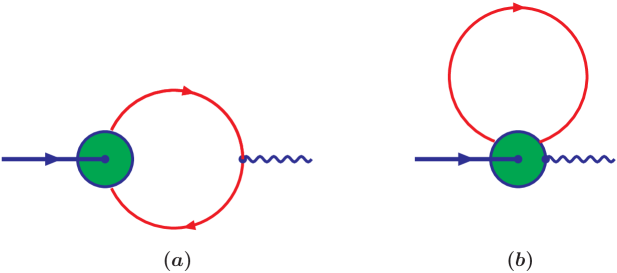
Figure 1: The diagrams corresponding to the $J/\psi\to\gamma$ transition: (a) the usual one and (b) the ”tadpole”.

For the pseudoscalar and vector mesons treated in this paper the derivatives of the mass operators are written as

$$\tilde{\Pi}^{\prime}_{P}(p^{2}) = \frac{1}{2p^{2}}\,p^{\alpha}\frac{d}{dp^{\alpha}}\,\int\!\!\frac{d^{4}k}{4\pi^{2}i}\tilde{\Phi}^{2}_{P}(-k^{2}){\rm tr}\biggl{[}\gamma^{5}S_{1}(\not\!k+c^{1}_{12}\not\!p)\gamma^{5}S_{2}(\not\!k-c^{2}_{12}\not\!p)\biggr{]},$$

$$\tilde{\Pi}^{\prime}_{V}(p^{2}) = \frac{1}{3}\biggl{[}g^{\mu\nu}-\frac{p^{\mu}p^{\nu}}{p^{2}}\biggr{]}\frac{1}{2p^{2}}\,p^{\alpha}\frac{d}{dp^{\alpha}}\,\int\!\!\frac{d^{4}k}{4\pi^{2}i}\tilde{\Phi}^{2}_{V}(-k^{2}){\rm tr}\biggl{[}\gamma^{\nu}S_{1}(\not\!k+c^{1}_{21}\not\!p)\gamma^{\mu}S_{2}(\not\!k-c^{2}_{12}\not\!p)\biggr{]}.$$

The leptonic decay constants $f_{P}$ and $f_{V}$ are

$$\frac{3g_{P}}{4\pi^{2}}\,\int\!\!\frac{d^{4}k}{4\pi^{2}i}\tilde{\Phi}_{P}(-k^{2}){\rm tr}\biggl{[}\gamma^{\mu}\gamma^{5}S_{1}(\not\!k+c^{1}_{12}\not\!p)\gamma^{5}S_{2}(\not\!k-c^{2}_{12}\not\!p)\biggr{]}=f_{P}\,p^{\mu}\,,$$

$$\frac{3g_{V}}{4\pi^{2}}\,\int\!\!\frac{d^{4}k}{4\pi^{2}i}\tilde{\Phi}_{V}(-k^{2}){\rm tr}\biggl{[}\gamma^{\mu}S_{1}(\not\!k+c^{1}_{12}\not\!p)\gamma\cdot\epsilon_{V}S_{2}(\not\!k-c^{2}_{12}\not\!p)\biggr{]}=m_{V}\,f_{V}\,\epsilon_{V}^{\mu}\,.$$

We use free fermion propagators for the valence quarks

$$S_{i}(\not\!k)=\frac{1}{m_{i}-\not\!k}$$ (10)

with an effective constituent quark mass $m_{i}$. As discussed in model-1 ; model-2 we assume for the meson mass $M_{H}$ that

$$M_{H}<m_{1}+m_{2}$$ (11)

in order to avoid the appearance of imaginary parts in the physical amplitudes. This holds true for the light pseudoscalar mesons but is no longer true for the light vector mesons. We shall therefore employ identical masses for the pseudoscalar mesons and the vector mesons in our matrix element calculations but use physical masses in the phase space calculation. This is quite a reliable approximation for the heavy vector mesons, e.g. $D^{\ast}$ and $B^{\ast}$, where the hyperfine splitting between the $D^{\ast}$ and $D$ and the $B^{\ast}$ and $B$, respectively, is quite small.

The shape of the vertex functions and the quark propagators can in principle be found from an analysis of the Bethe-Salpeter and Dyson-Schwinger equations as was done, e.g., in Roberts:dr ; Ivanov:1998ms . In this paper, however, we choose a phenomenological approach where the vertex functions are modeled by a Gaussian form, the size parameter of which is determined by a fit to the leptonic and radiative decays of the lowest-lying light, charm, and bottom mesons (see Table 1). Our previous studies of phenomena involving the low-lying hadrons have shown that this approximation is successful and reliable model-1 ; model-2 . We employ a Gaussian for the vertex function of the form $\tilde{\Phi}_{H}(k^{2}_{E})\doteq\exp(-k^{2}_{E}/\Lambda^{2}_{H})$, where $k_{E}$ is a Euclidean momentum. The size parameters $\Lambda^{2}_{H}$ are determined by a fit to experimental data, when available, or to lattice results for the leptonic decay constants $f_{P}$ and $f_{V}$ where $P=\pi,D,B$ and $V=J/\psi,\Upsilon$. Here we improve the fit by using the MINUIT code in a least-squares fit. The values of the fit parameters are displayed in Table 2. The quality of the fit may be assessed from the entries in Table 1.

$\begin{array}[]{||c|c|c||c|c|c|}\hline\cr\hline\cr&\mbox{This model}&\mbox{Expt. or lattice}&&\mbox{This model}&\mbox{Expt. or lattice}\\ \hline\cr\hline\cr f_{\pi}&130.7&130.7\pm 0.1\pm 0.36&g_{\pi^{0}\gamma\gamma}&0.272\mbox{ GeV${}^{-1}$}&0.273\mbox{ GeV${}^{-1}$}\\ \hline\cr f_{K}&159.8&159.8\pm 1.4\pm 0.44&f_{J/\psi}&405&405\pm 17\\ \hline\cr f_{D}&211&\begin{array}[]{c}203\pm 14\\ 226\pm 15\end{array}&f_{B}&182&\begin{array}[]{c}173\pm 23\\ 198\pm 30\end{array}\\ \hline\cr f_{D_{s}}&244&\begin{array}[]{c}230\pm 14\\ 250\pm 30\end{array}&f_{B_{s}}&209&\begin{array}[]{c}200\pm 20\\ 230\pm 30\end{array}\\ \hline\cr f_{B_{c}}&360&360&f_{\Upsilon}&710&710\pm 37\\ \hline\cr\hline\cr\hline\cr\end{array}$

Table 1: The physical quantities used in least-squares fitting our parameters. The values are taken from the Particle Data Group PDB or from lattice simulations Ryan . The value of $f_{B_{c}}$ is our average of QCD sum rules calculations QCDSR . All numbers are given in MeV except for $g_{\pi^{0}\gamma\gamma}$.

$\begin{array}[]{||c|c||c|c||c|c||}\hline\cr\hline\cr\mbox{Quark masses}&\mbox{(GeV)}&\Lambda_{H}&\mbox{(GeV)}&\Lambda_{H}&\mbox{(GeV)}\\ \hline\cr\hline\cr m_{u}=m_{d}&0.223&\Lambda_{\pi}&1.074&\Lambda_{B_{c}}&1.959\\ \hline\cr m_{s}&0.356&\Lambda_{K}&1.514&\Lambda_{J/\psi}&2.622\\ \hline\cr m_{c}&1.707&\Lambda_{D}=\Lambda_{D_{s}}&1.844&\Lambda_{\Upsilon}&3.965\\ \hline\cr m_{b}&5.121&\Lambda_{B}=\Lambda_{B_{s}}&1.887&&\\ \hline\cr\hline\cr\end{array}$

Table 2: The fitted values of the model parameters.

III Strong triangle and box diagrams

Transition matrix elements involving composite hadrons are specified in the model by the appropriate quark diagram. Here, we give explicit expressions for the integrals corresponding to the strong triangle and box diagrams shown in Fig. 2.

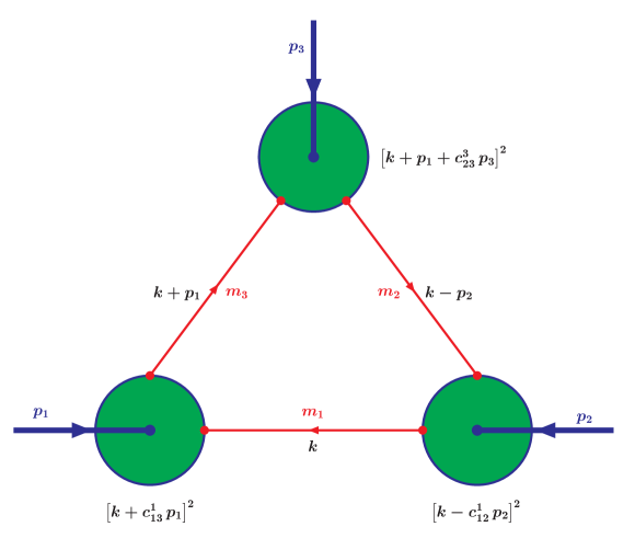
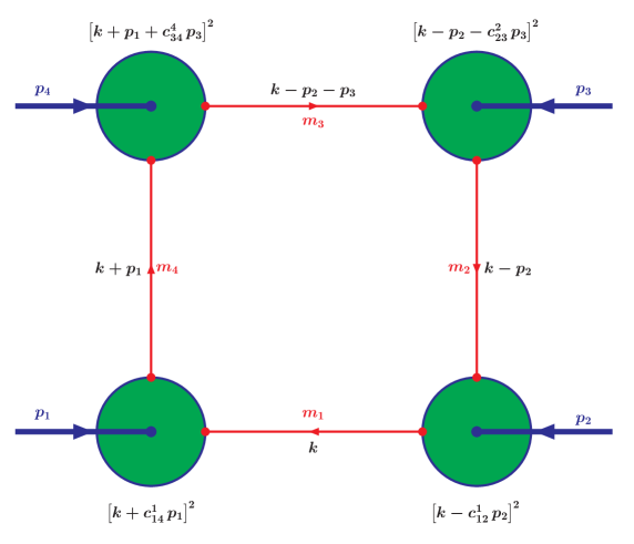
Figure 2: The strong triangle and box diagrams.

First, we will make the transformations which are common for all one-loop diagrams with local propagators and Gaussian vertex functions. The Feynman integral corresponding to a one-loop diagram with $n$ propagators and, respectively, $n$ vertex functions may be written in Minkowskii space as

$$I_{n}(p_{1},...,p_{n})=\int\!\!\frac{d^{4}k}{4\pi^{2}i}\,{\rm tr}\left[\prod\limits_{i=1}^{n}\tilde{\Phi}_{i}\left(-(k+v_{i+n})^{2}\right)\,\Gamma_{i}\,S_{i}(\not\!k+\not\!v_{i})\right]$$ (12)

where the vectors $v_{i}$ are linear combinations of the external momenta $p_{i}$ to be specified later on, $k$ is the loop momentum, and $\Gamma_{i}$ are Dirac matrices for the $i$ meson (cf. Eq. (1)). The external momenta are all chosen as ingoing such that one has $\sum\limits_{i=1}^{n}p_{i}=0$.

The propagators can be written as

$$S_{i}(\not\!k+\not\!v_{i}) = (m_{i}+\not\!k+\not\!v_{i})\cdot\int\limits_{0}^{\infty}\!d\beta_{i}\,e^{-\beta_{i}\,(m^{2}_{i}-(k+v_{i})^{2})}\,.$$ (13)

For the vertex functions one writes

$$\tilde{\Phi}_{i}\left(-(k+v_{i+n})^{2}\right) = e^{\beta_{i+n}\cdot(k+v_{i+n})^{2}}\hskip 28.45274pti=1,...,n\,,$$ (14)

where the parameters $\beta_{i+n}=s_{i}=1/\Lambda^{2}_{i}$ are the size parameters. One can then easily perform the integration over $k$:

$$\int\!\!\frac{d^{4}k}{\pi^{2}i}\,\exp\left\{\sum\limits_{i=1}^{2\,n}\beta_{i}\,(k+v_{i})^{2}\right\}=\frac{1}{\beta^{2}}\exp\left\{\frac{1}{\beta}\sum\limits_{1\leq i<j\leq 2\,n}\beta_{i}\,\beta_{j}\,(v_{i}-v_{j})^{2}\right\}\,.$$ (15)

Here, $\beta=\sum\limits_{i=1}^{2\,n}\beta_{i}$. The numerator $m_{i}\,+\!\not\!k\,+\!\not\!v_{i}$ can be replaced by a differential operator in the following manner:

$$\int\!\!\frac{d^{4}k}{\pi^{2}i}\,\prod\limits_{i=1}^{n}\Gamma_{i}\left(m_{i}+\not\!k+\not\!v_{i}\right)e^{\beta k^{2}+2kr} = \prod\limits_{i=1}^{n}\Gamma_{i}\left(m_{i}+\not\!v_{i}+\frac{1}{2}\not\!\partial_{r}\right)\cdot\frac{1}{\beta^{2}}e^{-r^{2}/\beta}$$

$$= \frac{1}{\beta^{2}}e^{-r^{2}/\beta}\prod\limits_{i=1}^{n}\Gamma_{i}\left(m_{i}+\not\!v_{i}-\frac{1}{\beta}\not\!r+\frac{1}{2}\not\!\partial_{r}\right).$$

We thus have

$$I_{n}(p_{1},...,p_{n}) = \prod\limits_{i=1}^{n}\int\limits_{0}^{\infty}\frac{d\beta_{i}}{\beta^{2}}\times\exp\left\{-\sum\limits_{i=1}^{n}\beta_{i}m^{2}_{i}+\frac{1}{\beta}\sum\limits_{1\leq i<j\leq 2\,n}\beta_{i}\,\beta_{j}\,(v_{i}-v_{j})^{2}\right\}$$

$$\times \frac{1}{4}{\rm tr}\,\left[\prod\limits_{i=1}^{n}\Gamma_{i}\left(m_{i}+\not\!v_{i}-\frac{1}{\beta}\not\!r+\frac{1}{2}\not\!\partial_{r}\right)\right]\,,$$

where $r=\sum\limits_{i=1}^{2\,n}\beta_{i}\,v_{i}$. Finally, we effect some further transformations on the integration variables to get the integral into a form suitable for numerical evaluation:

• we use the formula

  $$\prod\limits_{i=1}^{n}\int\limits_{0}^{\infty}\!d\beta_{i}\,f(\beta_{1},...,\beta_{n})=\int\limits_{0}^{\infty}\!dt\,t^{n-1}\prod\limits_{i=1}^{n}\int\limits_{0}^{\infty}\!d\alpha_{i}\,\delta\left(1-\sum\limits_{i=1}^{n}\alpha_{i}\right)f(t\,\alpha_{1},...,t\,\alpha_{n})\,;$$

• we scale the $t$ variable by $t\to w\,t$ with $w=\sum\limits_{i=1}^{n}\beta_{i+n}=\sum\limits_{i=1}^{n}\,s_{i}$ and introduce the new variable $\tilde{\beta}_{i}=\beta_{i}/w$ ($i=n+1,...,2n)$.

We have

$$I_{n}(p_{1},...,p_{n}) = \int\limits_{0}^{\infty}\!dt\frac{t^{n-1}}{(1+t)^{2}}\prod\limits_{i=1}^{n}\int\limits_{0}^{\infty}\!d\alpha_{i}\,\delta\left(1-\sum\limits_{i=1}^{n}\alpha_{i}\right)\cdot e^{-w\,z}$$

$$\times \frac{w^{2}}{4}{\rm tr}\,\left[\prod\limits_{i=1}^{n}\Gamma_{i}\left(m_{i}+\not\!v_{i}-\frac{1}{1+t}\not\!\tilde{r}+\frac{1}{2\,w}\not\!\partial_{\tilde{r}}\right)\right]\,,$$

where

$$\tilde{r}=t\,\sum_{i=1}^{n}\alpha_{i}\,v_{i}+\sum_{i=n+1}^{2\,n}\tilde{\beta}_{i}\,v_{i}\,.$$

The $z$ form in the exponential function is written as

$$z = t\,z_{\,\rm loc}-\frac{t}{1+t}\,z_{1}-\frac{1}{1+t}\,z_{2}\,,$$ (19)

$$z_{\,\rm loc} = \sum_{i=1}^{n}\alpha_{i}\,m^{2}_{i}-\sum_{1\leq i<j\leq n}\alpha_{i}\,\alpha_{j}\,a_{ij}\,,$$

$$z_{1} = \sum_{i=1}^{n}\alpha_{i}\,\sum_{j=n+1}^{2\,n}\tilde{\beta}_{j}\,a_{ij}-\sum_{1\leq i<j\leq n}\alpha_{i}\,\alpha_{j}\,a_{ij}\,,$$

$$z_{2} = \sum_{n+1\leq i<j\leq 2\,n}\tilde{\beta}_{i}\,\tilde{\beta}_{j}\,a_{ij}\,.$$

The matrix $a_{ij}=(v_{i}-v_{j})^{2}$ depends on the invariant kinematical variables. Explicit expressions for this matrix for the triangle and box diagrams are given in Tables 3 and 4, respectively. We will introduce the variable $v=t/(1+t)$ ($0\leq v\leq 1$) in Eq. (III) in what follows.

$a_{12}=p_{2}^{2}$	$a_{13}=p_{1}^{2}$	$a_{23}=p_{3}^{2}$
$a_{14}=\left(c_{13}^{1}\right)^{2}p_{1}^{2}$	$a_{15}=\left(c_{12}^{1}\right)^{2}p_{2}^{2}$	$a_{16}=c_{23}^{2}\,p_{1}^{2}-c_{23}^{2}\,c_{23}^{3}\,p_{3}^{2}+c_{23}^{3}\,p_{2}^{2}$
$a_{24}=c_{13}^{3}\,p_{2}^{2}-c_{13}^{1}\,c_{13}^{3}\,p_{1}^{2}+c_{13}^{1}\,p_{3}^{2}$	$a_{25}=\left(c_{12}^{2}\right)^{2}p_{2}^{2}$	$a_{26}=\left(c_{23}^{2}\right)^{2}p_{3}^{2}$
$a_{34}=\left(c_{13}^{3}\right)^{2}p_{1}^{2}$	$a_{35}=c_{12}^{2}\,p_{1}^{2}-c_{12}^{1}\,c_{12}^{2}\,p_{2}^{2}+c_{12}^{1}\,p_{3}^{2}$	$a_{36}=\left(c_{23}^{3}\right)^{2}p_{3}^{2}$
$a_{45}=c_{13}^{1}\,(c_{13}^{1}-c_{12}^{1})\,p_{1}^{2}$	$a_{46}=c_{13}^{3}\,(c_{13}^{3}-c_{23}^{3})\,p_{1}^{2}$	$a_{56}=c_{12}^{2}\,(c_{12}^{2}-c_{23}^{2})\,p_{2}^{2}$
$+c_{12}^{1}\,(c_{12}^{1}-c_{13}^{1})\,p_{2}^{2}+c_{12}^{1}\,c_{13}^{1}\,p_{3}^{2}$	$+c_{23}^{3}\,(c_{23}^{3}-c_{13}^{3})\,p_{2}^{2}+c_{13}^{3}\,c_{23}^{3}\,p_{3}^{2}$	$+c_{23}^{2}\,(c_{23}^{2}-c_{12}^{2})\,p_{3}^{2}+c_{12}^{2}\,c_{23}^{2}\,p_{1}^{2}$

Table 3: The matrix $a_{ij}=(v_{i}-v_{j})^{2}$ for the triangle diagram. Here, $v_{1}=0$, $v_{2}=-p_{2}$, $v_{3}=p_{1}$, $v_{4}=c_{13}^{1}\,p_{1}$, $v_{5}=-c_{12}^{1}\,p_{2}$, $v_{6}=p_{1}+c_{23}^{3}\,p_{3}$.

$a_{12}=p_{2}^{2}$	$a_{13}=(p_{2}+p_{3})^{2}$	$a_{14}=p_{1}^{2}$
$a_{23}=p_{3}^{2}$	$a_{24}=(p_{1}+p_{2})^{2}$	$a_{34}=p_{4}^{2}$
$a_{15}=\left(c_{14}^{1}\right)^{2}p_{1}^{2}$	$a_{16}=\left(c_{12}^{1}\right)^{2}p_{2}^{2}$	$a_{17}=c_{23}^{3}\,p_{2}^{2}-c_{23}^{2}\,c_{23}^{3}\,p_{3}^{2}$
		$+c_{23}^{2}\,(p_{2}+p_{3})^{2}$
$a_{18}=c_{34}^{3}\,p_{1}^{2}-c_{34}^{3}\,c_{34}^{4}\,p_{4}^{2}$	$a_{25}=c_{14}^{4}p_{2}^{2}-c_{14}^{1}\,c_{14}^{4}\,p_{1}^{2}$	$a_{26}=\left(c_{12}^{2}\right)^{2}p_{2}^{2}$
$+c_{34}^{4}\,(p_{1}+p_{4})^{2}$	$+c_{14}^{1}\,(p_{1}+p_{2})^{2}$
$a_{27}=\left(c_{23}^{2}\right)^{2}p_{3}^{2}$	$a_{28}=c_{34}^{4}\,p_{3}^{2}-c_{34}^{3}\,c_{34}^{4}\,p_{4}^{2}$	$a_{35}=c_{14}^{1}\,p_{4}^{2}-c_{14}^{1}\,c_{14}^{4}\,p_{1}^{2}$
	$+c_{34}^{3}\,(p_{3}+p_{4})^{2}$	$+c_{14}^{4}\,(p_{1}+p_{4})^{2}$
$a_{36}=c_{12}^{1}\,p_{3}^{2}-c_{12}^{1}\,c_{12}^{2}\,p_{2}^{2}+c_{12}^{2}\,(p_{2}+p_{3})^{2}$	$a_{37}=\left(c_{23}^{3}\right)^{2}p_{3}^{2}$	$a_{38}=\left(c_{34}^{3}\right)^{2}p_{4}^{2}$
$a_{45}=\left(c_{14}^{4}\right)^{2}p_{1}^{2}$	$a_{46}=c_{12}^{2}\,p_{1}^{2}-c_{12}^{1}\,c_{12}^{2}\,p_{2}^{2}$	$a_{47}=c_{23}^{2}\,p_{4}^{2}-c_{23}^{2}\,c_{23}^{3}\,p_{3}^{2}$
	$+c_{12}^{1}\,(p_{1}+p_{2})^{2}$	$+c_{23}^{3}\,(p_{3}+p_{4})^{2}$
$a_{48}=\left(c_{34}^{4}\right)^{2}p_{4}^{2}$

Table 4: The matrix $a_{ij}=(v_{i}-v_{j})^{2}$ for the box diagram. Here, $v_{1}=0$, $v_{2}=-p_{2}$, $v_{3}=-p_{2}-p_{3}$, $v_{4}=p_{1}$, $v_{5}=c_{14}^{1}\,p_{1}$, $v_{6}=-c_{12}^{1}\,p_{2}$, $v_{7}=-p_{2}-c_{23}^{2}\,p_{3}$, $v_{8}=p_{1}+c_{34}^{4}\,p_{4}$.

Some further remarks are appropriate. One can see that the existence of the loop integral Eq. (III) is defined by the local $\alpha$ form $z_{\,\rm loc}$. Even if we apply the constraints Eq. (11) it does not guarantee that this form is always positive. For instance, in the simplest triangle diagram with $p_{1}^{2}=p_{2}^{2}=p_{3}^{2}\equiv p^{2}$ and $m_{1}=m_{2}=m_{3}=m$ the form $z_{\,\rm loc}=0$ if $p^{2}=3m^{2}$. Such singularities in the Feynman diagrams with local propagators are called anomalous thresholds (see the discussion in Ref. Davydychev:2001uj and other references therein). The situation is much more complicated in the case of the box diagrams. Obviously, we cannot consider the annihilation processes when the energy is large enough to go beyond the normal thresholds corresponding to quark production. However, in the case of the dissociation processes considered here, the local form $z_{\,\rm loc}$ is always positive, and we are able to make self-consistent and reliable predictions for physical observables.

IV The $J/\psi$ dissociation amplitudes and cross sections

In our approach the dissociation processes $J/\psi+\pi^{+}\to D+\overline{D^{0}}$, $D^{\ast\,+}+\overline{D^{0}}$, and $D^{\ast\,+}+\overline{D^{\ast\,0}}$ are described by the diagrams in Fig. 3.

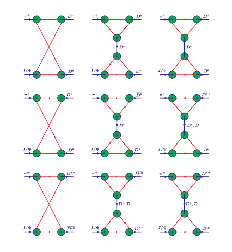
Figure 3: The Feynman diagrams describing the charm dissociation processes $J/\psi+\pi^{+}\to D^{+}+\overline{D^{0}}$, $D^{\ast\,+}+\overline{D^{0}}$, $D^{\ast\,+}+\overline{D^{\ast\,0}}$.

Our momentum labeling is defined by

$$J/\psi(p_{1})+\pi^{+}(p_{2})\to D^{+}_{3}(q_{1})+\overline{D_{4}^{0}}(q_{2})$$ (20)

where $D_{3}^{+}=D^{+}$ or $D^{\ast\,+}$, $\overline{D_{4}^{0}}=\overline{D^{0}}$ or $\overline{D^{\ast\,0}}$, $p_{1}^{2}=m_{H1}^{2}\equiv m_{J/\psi}^{2}$, $p_{2}^{2}=m_{H2}^{2}\equiv m_{\pi}^{2}$, $q_{1}^{2}=m_{H3}^{2}\equiv m^{2}_{D^{+}}\,(m^{2}_{D^{\ast\,+}})$, $q_{2}^{2}=m_{H4}^{2}\equiv m^{2}_{\overline{D^{0}}}\,(m^{2}_{\overline{D^{\ast\,0}}})$.

The Mandelstam variables are defined in the standard form

$$s = (p_{1}+p_{2})^{2}=(q_{1}+q_{2})^{2},$$

$$t = (p_{1}-q_{1})^{2}=(p_{2}-q_{2})^{2},$$

$$u = (p_{1}-q_{2})^{2}=(p_{2}-q_{1})^{2},$$

where $s+t+u=m_{H1}^{2}+m_{H2}^{2}+m_{H3}^{2}+m_{H4}^{2}$.

Cross sections are calculated by using the formula

$$\sigma(s)=\frac{1}{192\pi s}\frac{1}{p^{2}_{1,\rm cm}}\int\limits_{t_{-}}^{t_{+}}\!dt\,|M(s,t)|^{2}$$ (21)

where $M(s,t)$ is an invariant amplitude and

$$t_{\pm} = (E_{1,\rm cm}-E_{3,\rm cm})^{2}-(p_{1,\rm cm}\mp q_{1,\rm cm})^{2},$$

$$E_{1,\rm cm} = \frac{s+m^{2}_{H1}-m^{2}_{H2}}{2\sqrt{s}},\hskip 28.45274ptE_{3,\rm cm}=\frac{s+m^{2}_{H3}-m^{2}_{H4}}{2\sqrt{s}},$$

$$p_{1,\rm cm} = \frac{\lambda^{1/2}(s,m^{2}_{H1},m^{2}_{H2})}{2\sqrt{s}},\hskip 28.45274ptq_{1,\rm cm}=\frac{\lambda^{1/2}(s,m^{2}_{H3},m^{2}_{H4})}{2\sqrt{s}}.$$

The reaction threshold is equal to $s_{0}=(m_{H3}+m_{H4})^{2}$. Note that Eq. (21) contains the statistical factor 1/3 which comes from averaging over the initial state $J/\psi$ polarizations.

The dissociation processes are described by both the box and the resonance diagrams as shown in Fig. 3. The resonance diagrams depend explicitly only on the $t$ or $u$ variables whereas the box diagrams are functions of $s$ and $t$.

In the following three subsections we write explicitly the amplitudes for the processes $J/\psi+\pi^{+}\to D^{+}+\overline{D^{0}}$, $D^{\ast\,+}+\overline{D^{0}}$, $D^{\ast\,+}+\overline{D^{\ast\,0}}$ in terms of form factors; all the analytical expressions for them are reported.

IV.1 The channel $J/\psi+\pi^{+}\to D^{+}+\overline{D^{0}}$

The invariant matrix element is written as

$$M({\rm VPPP})=M_{\Box}({\rm VPPP})\,+\,M_{\rm res}({\rm VPPP}),$$ (22)

where

$$M_{\Box}({\rm VPPP}) = \epsilon_{\mu_{1}}(p_{1})\cdot\varepsilon^{\mu_{1}p_{1}p_{2}q_{2}}\,F_{\rm VPPP}(s,t),$$ (23)

$$M_{\rm res}({\rm VPPP}) = \epsilon_{\mu_{1}}(p_{1})\cdot\left\{-\,M^{\alpha}_{\triangle\,a}({\rm PVP})\,D^{\alpha\beta}_{D^{\ast}}(p_{2}-q_{2})\,M^{\mu_{1}\beta}_{\triangle\,a}({\rm VVP})\right.$$

$$- \left.M^{\alpha}_{\triangle\,b}({\rm PPV})\,D^{\alpha\beta}_{D^{\ast}}(p_{2}-q_{1})\,M^{\mu_{1}\beta}_{\triangle,b}({\rm VPV})\right\}\,,$$

$$M^{\alpha}_{\triangle\,a}({\rm PVP}) = p_{2}^{\alpha}\,F^{(1a)}_{\rm PVP}(t),\hskip 28.45274ptM^{\mu_{1}\beta}_{\triangle\,a}({\rm VVP})=\varepsilon^{\mu_{1}\beta p_{1}(p_{2}-q_{2})}\,F^{(a)}_{\rm VVP}(t),$$

$$M^{\alpha}_{\triangle\,b}({\rm PPV}) = p_{2}^{\alpha}\,F^{(1b)}_{\rm PPV}(u),\hskip 28.45274ptM^{\mu_{1}\beta}_{\triangle\,b}({\rm VPV})=\varepsilon^{\mu_{1}\beta p_{1}(p_{2}-q_{1})}\,F^{(b)}_{\rm VPV}(u).$$

The common minus sign is due to the extra quark loop in the resonance diagrams as compared to the box diagram. This extra sign is very important, as will be seen later on, since the extra sign leads to a constructive interference of resonance and box graph contributions. The loop momenta directions come from explicit calculation of the S-matrix elements and are shown in Fig. 3. The vector ($D^{\ast}$) and pseudoscalar ($D$) meson propagators are given by

$$D^{\alpha\beta}_{D^{\ast}}(p)=\frac{-g^{\alpha\beta}+p^{\alpha}p^{\beta}/m^{2}_{D^{\ast}}}{m^{2}_{D^{\ast}}-p^{2}},\hskip 28.45274pti^{2}D_{D}(p)=\frac{-1}{m^{2}_{D}-p^{2}}.$$

For the form factors one obtains

$$F_{\rm VPPP}(s,t) = g_{J/\psi}\,g^{2}_{D}\,g_{\pi}\int\!d\sigma_{\Box}\cdot\exp(-w\cdot z_{\Box}(s,t))\cdot w^{2}\,(m_{c}\,(1+d_{2})-m_{q}\,d_{2}),$$

$$F^{(1a)}_{\rm PVP}(t) = g_{\pi}\,g_{D^{\ast}}\,g_{D}\,\int\!d\sigma_{\triangle}\cdot\exp(-wz_{\triangle}(t))\,\cdot[w\,(-m_{q}\,m_{c}-m_{q}^{2}\,b_{1}$$

$$+m^{2}_{\pi}\,b_{1}^{2}\,(b_{1}+b_{2}-1)-m^{2}_{D}\,b_{1}^{2}\,b_{2}$$

$$+t\,b_{2}\,(b_{1}\,b_{2}+b_{1}^{2}-1+b_{2}))$$

$$-(1-v)\,(1+3\,b_{1})],$$

$$F^{(a)}_{\rm VVP}(t) = g_{J/\psi}\,g_{D^{\ast}}\,g_{D}\,\int\!d\sigma_{\triangle}\cdot\exp(-wz_{\triangle}(t))\,\cdot[w\,(m_{c}\,(b_{2}-1)-m_{q}\,b_{2})],$$

$$F^{(1b)}_{\rm PPV}(u) = g_{\pi}\,g_{D^{\ast}}\,g_{D}\,\int d\sigma_{\triangle}\cdot\exp(-wz_{\triangle}(u))\,\cdot[w\,(m_{q}\,m_{c}+m_{q}^{2}\,(1-b_{1}-b_{2})$$

$$+m^{2}_{\pi}\,(-2\,b_{1}\,b_{2}+b_{1}\,b_{2}^{2}+b_{1}+2\,b_{1}^{2}\,b_{2}-2\,b_{1}^{2}+b_{1}^{3})$$

$$+m^{2}_{D}\,(-2\,b_{1}\,b_{2}+2\,b_{1}\,b_{2}^{2}+b_{1}^{2}\,b_{2}+b_{2}-2\,b_{2}^{2}+b_{2}^{3})$$

$$+u\,(2\,b_{1}\,b_{2}-b_{1}\,b_{2}^{2}-b_{1}^{2}\,b_{2}))$$

$$+4+3\,b_{1}\,v-3\,b_{1}+3\,b_{2}\,v-3\,b_{2}-4\,v],$$

$$F^{(b)}_{\rm VPV}(u) = g_{J/\psi}\,g_{D}\,g_{D^{\ast}}\,\int\!d\sigma_{\triangle}\cdot\exp(-wz_{\triangle}(u))\cdot[w\,(-m_{c}+b_{2}\,(m_{c}-m_{q}))].$$

The integration measures are defined by

$$\int\!d\sigma_{\Box} = \frac{3}{4\pi^{2}}\,\int\limits_{0}^{1}dv\left(\frac{v}{1-v}\right)^{3}\int d^{4}\alpha\,\delta\left(1-\sum\limits_{i=1}^{4}\alpha_{i}\right),$$

$$\int d\sigma_{\triangle} = \frac{3}{4\pi^{2}}\,\int\limits_{0}^{1}\!dv\left(\frac{v}{1-v}\right)^{2}\int d^{3}\alpha\,\delta\left(1-\sum\limits_{i=1}^{3}\alpha_{i}\right).$$

The coefficients $b_{i}$ (triangle diagrams) and $d_{i}$ (box diagrams) are given by

$$b_{1} = v\,\alpha_{3}+(1-v)\,(\tilde{s}_{1}\,c_{13}^{1}+\tilde{s}_{3}\,c_{23}^{2}),$$

$$b_{2} = v\,\alpha_{2}+(1-v)\,(\tilde{s}_{2}\,c_{12}^{1}+\tilde{s}_{3}\,c_{23}^{3}),$$

$$d_{1} = v\,\alpha_{4}+(1-v)\,(\tilde{s}_{1}\,c_{14}^{1}+\tilde{s}_{4}\,c_{34}^{3}),$$

$$d_{2} = -\,v\,(\alpha_{2}+\alpha_{3})-(1-v)\,(\tilde{s}_{2}\,c_{12}^{1}+\tilde{s}_{3}+\tilde{s}_{4}\,c_{34}^{4}),$$

$$d_{3} = -\,v\,\alpha_{3}-(1-v)\,(\tilde{s}_{3}\,c_{23}^{2}+\tilde{s}_{3}+\tilde{s}_{4}\,c_{34}^{4})\,.$$

The values of $z_{\triangle}$, $z_{\Box}$, and $w$ are defined by the relevant diagrams (size parameters and quark and hadron masses).

IV.2 The channel $J/\psi+\pi^{+}\to D^{\ast\,+}+\overline{D^{0}}$

The invariant matrix element can be written as:

$$M({\rm VPPV})=M_{\Box}({\rm VPPV})\,+\,M_{\rm res}({\rm VPPV})\,,$$ (25)

with

$$M_{\Box}({\rm VPPV}) = \epsilon_{\mu_{1}}(p_{1})\epsilon_{\mu_{2}}(q_{1})\cdot\left(p_{2}^{\mu_{1}}\,p_{1}^{\mu_{2}}\,F^{(1)}_{\rm VPPV}(s,t)+q_{2}^{\mu_{1}}\,p_{1}^{\mu_{2}}\,F^{(2)}_{\rm VPPV}(s,t)\right.$$

$$+ \left.p_{2}^{\mu_{1}}\,p_{2}^{\mu_{2}}\,F^{(3)}_{\rm VPPV}(s,t)+q_{2}^{\mu_{1}}\,p_{2}^{\mu_{2}}\,F^{(4)}_{\rm VPPV}(s,t)+g^{\mu_{1}\mu_{2}}\,F^{(5)}_{\rm VPPV}(s,t)\right)\,,$$

$$M_{\rm res}({\rm VPPV}) = \epsilon_{\mu_{1}}(p_{1})\epsilon_{\mu_{2}}(q_{1})$$

$$\times \left(-\,M^{\alpha}_{\triangle\,a}({\rm PVP})\,D^{\alpha\beta}_{D^{\ast}}(p_{2}-q_{2})\,M^{\mu_{1}\beta\mu_{2}}_{\triangle\,a}({\rm VVV})-\,M^{\alpha\mu_{2}}_{\triangle\,b}({\rm PVV})\,D^{\alpha\beta}_{D^{\ast}}(p_{2}-q_{1})\,M^{\mu_{1}\beta}_{\triangle,b}({\rm VPV})\right.$$

$$+ \left.M^{\mu_{2}}_{\triangle\,c}({\rm PVP})\,D_{D}(p_{2}-q_{1})\,M^{\mu_{1}}_{\triangle,c}({\rm VPP})\right)\,.$$

The expressions for the form factors are given in the Appendix.

IV.3 The channel $J/\psi+\pi^{+}\to D^{\ast\,+}+\overline{D^{\ast\,0}}$

The amplitude for the process $J/\psi+\pi^{+}\to D^{\ast\,+}+\overline{D^{\ast\,0}}$ can be written as

$$M({\rm VVPV})=M_{\Box}({\rm VVPV})\,+\,M_{\rm res}({\rm VVPV}),$$ (26)

where

$$M_{\Box}({\rm VVPV}) = \epsilon_{\mu_{1}}(p_{1})\epsilon_{\mu_{2}}(q_{2})\epsilon_{\mu_{3}}(q_{1})$$

$$\times \left(g^{\mu_{2}\mu_{3}}\varepsilon^{p_{1}p_{2}q_{2}\mu_{1}}\,F^{(1)}_{\rm VVPV}(s,t)+g^{\mu_{1}\mu_{3}}\varepsilon^{p_{1}p_{2}q_{2}\mu_{2}}\,F^{(2)}_{\rm VVPV}(s,t)+g^{\mu_{1}\mu_{2}}\varepsilon^{p_{1}p_{2}q_{2}\mu_{3}}\,F^{(3)}_{\rm VVPV}(s,t)\right.$$

$$+p_{1}^{\mu_{3}}\varepsilon^{p_{1}p_{2}\mu_{1}\mu_{2}}\,F^{(4)}_{\rm VVPV}(s,t)+p_{1}^{\mu_{2}}\varepsilon^{p_{1}p_{2}\mu_{1}\mu_{3}}\,F^{(5)}_{\rm VVPV}(s,t)+p_{2}^{\mu_{3}}\varepsilon^{p_{1}p_{2}\mu_{1}\mu_{2}}\,F^{(6)}_{\rm VVPV}(s,t)$$

$$+p_{2}^{\mu_{2}}\varepsilon^{p_{1}p_{2}\mu_{1}\mu_{3}}\,F^{(7)}_{\rm VVPV}(s,t)+p_{2}^{\mu_{1}}\varepsilon^{p_{1}p_{2}\mu_{2}\mu_{3}}\,F^{(8)}_{\rm VVPV}(s,t)+q_{2}^{\mu_{1}}\varepsilon^{p_{1}p_{2}\mu_{2}\mu_{3}}\,F^{(9)}_{\rm VVPV}(s,t)$$

$$+p_{2}^{\mu_{2}}\varepsilon^{p_{1}q_{2}\mu_{1}\mu_{3}}\,F^{(10)}_{\rm VVPV}(s,t)+p_{2}^{\mu_{3}}\varepsilon^{p_{1}q_{2}\mu_{1}\mu_{2}}\,F^{(11)}_{\rm VVPV}(s,t)+p_{1}^{\mu_{3}}\varepsilon^{p_{2}q_{2}\mu_{1}\mu_{2}}\,F^{(12)}_{\rm VVPV}(s,t)$$

$$+p_{1}^{\mu_{2}}\varepsilon^{p_{2}q_{2}\mu_{1}\mu_{3}}\,F^{(13)}_{\rm VVPV}(s,t)+p_{2}^{\mu_{1}}\varepsilon^{p_{2}q_{2}\mu_{2}\mu_{3}}\,F^{(14)}_{\rm VVPV}(s,t)+q_{2}^{\mu_{1}}\varepsilon^{p_{2}q_{2}\mu_{2}\mu_{3}}\,F^{(15)}_{\rm VVPV}(s,t)$$

$$\left.+\varepsilon^{p_{1}\mu_{1}\mu_{2}\mu_{3}}\,F^{(16)}_{\rm VVPV}(s,t)+\varepsilon^{p_{2}\mu_{1}\mu_{2}\mu_{3}}\,F^{(17)}_{\rm VVPV}(s,t)\right).$$

When taking into account parity invariance one knows from helicity counting that there are only 14 independent amplitudes in the $(VVPV)$ case. The above set of 17 amplitudes are in fact not independent. They can be reduced to a set of 14 independent amplitudes by making use of the Schouten identity (see, e.g., Korner:2003zq )

$$g^{\mu\mu_{1}}\varepsilon^{\mu_{2}\mu_{3}\mu_{4}\mu_{5}}+{\rm cycl.(\mu_{1},\mu_{2},\mu_{3},\mu_{4},\mu_{5})}=0.$$

We have made use of the Schouten identity as an additional check on our numerical calculations.

Moreover, the resonance term, $M_{\rm res}({\rm VVPV})$, and all the structures involved are reported in the following expressions:

$$M_{\rm res}({\rm VVPV}) = \epsilon_{\mu_{1}}(p_{1})\epsilon_{\mu_{2}}(q_{2})\epsilon_{\mu_{3}}(q_{1})$$

$$\times \left(-\,M^{\alpha\mu_{2}}_{\triangle\,a}({\rm PVV})\,D^{\alpha\beta}_{D^{\ast}}(p_{2}-q_{2})\,M^{\mu_{1}\beta\mu_{3}}_{\triangle\,a}({\rm VVV})-\,M^{\alpha\mu_{3}}_{\triangle\,b}({\rm PVV})\,D^{\alpha\beta}_{D^{\ast}}(p_{2}-q_{1})\,M^{\mu_{1}\beta\mu_{2}}_{\triangle,b}({\rm VVV})\right.$$

$$+ \left.M^{\mu_{2}}_{\triangle\,c}({\rm PPV})\,D_{D}(p_{2}-q_{2})\,M^{\mu_{1}\mu_{3}}_{\triangle,c}({\rm VPV})+\,M^{\mu_{3}}_{\triangle,d}({\rm PVP})\,D_{D}(p_{2}-q_{1})\,M^{\mu_{1}\mu_{2}}_{\triangle,d}({\rm VVP})\right)\,,$$

$$M^{\alpha\mu_{2}}_{\triangle\,a}({\rm PVV}) = \varepsilon^{p_{2}(p_{2}-q_{2})\mu_{2}\alpha}\,F^{(a)}_{\rm PVV}(t)\,,$$

$$M^{\mu_{1}\beta\mu_{3}}_{\triangle\,a}({\rm VVV}) = (p_{2}-q_{2})^{\mu_{1}}p_{1}^{\beta}p_{1}^{\mu_{3}}\,F^{(1a)}_{\rm VVV}(t)+(p_{2}-q_{2})^{\mu_{1}}(p_{2}-q_{2})^{\beta}p_{1}^{\mu_{3}}\,F^{(2a)}_{\rm VVV}(t)$$

$$+ g^{\mu_{1}\mu_{3}}p_{1}^{\beta}\,F^{(3a)}_{\rm VVV}(t)+g^{\mu_{1}\mu_{3}}(p_{2}-q_{2})^{\beta}\,F^{(4a)}_{\rm VVV}(t)$$

$$+ g^{\mu_{1}\beta}p_{1}^{\mu_{3}}\,F^{(5a)}_{\rm VVV}(t)+g^{\mu_{3}\beta}(p_{2}-q_{2})^{\mu_{1}}\,F^{(6a)}_{\rm VVV}(t)\,,$$

$$M^{\alpha\mu_{3}}_{\triangle\,b}({\rm PVV}) = \varepsilon^{p_{2}(p_{2}-q_{1})\mu_{3}\alpha}\,F^{(b)}_{\rm PVV}(u)\,,$$

$$M^{\mu_{1}\beta\mu_{2}}_{\triangle\,b}({\rm VVV}) = (p_{2}-q_{1})^{\mu_{1}}p_{1}^{\beta}p_{1}^{\mu_{2}}\,F^{(1b)}_{\rm VVV}(u)+(p_{2}-q_{1})^{\mu_{1}}(p_{2}-q_{1})^{\beta}p_{1}^{\mu_{2}}\,F^{(2b)}_{\rm VVV}(u)$$

$$+ g^{\mu_{1}\mu_{2}}p_{1}^{\beta}\,F^{(3b)}_{\rm VVV}(u)+g^{\mu_{1}\mu_{2}}(p_{2}-q_{1})^{\beta}\,F^{(4b)}_{\rm VVV}(u)$$

$$+ g^{\mu_{1}\beta}p_{1}^{\mu_{2}}\,F^{(5b)}_{\rm VVV}(u)+g^{\mu_{2}\beta}(p_{2}-q_{1})^{\mu_{1}}\,F^{(6b)}_{\rm VVV}(u)\,,$$

$$M^{\mu_{2}}_{\triangle\,c}({\rm PPV}) = p_{2}^{\mu_{2}}\,F^{(c)}_{\rm PPV}(t)\,,$$

$$M^{\mu_{1}\mu_{3}}_{\triangle,c}({\rm VPV}) = \varepsilon^{p_{1}q_{1}\mu_{1}\mu_{3}}\,F^{(c)}_{\rm VPV}(t)\,,$$

$$M^{\mu_{3}}_{\triangle,d}({\rm PVP})\, = p_{2}^{\mu_{3}}\,F^{(d)}_{\rm PVP}(u)$$

$$M^{\mu_{1}\mu_{2}}_{\triangle,d}({\rm VVP}) = \varepsilon^{p_{1}q_{2}\mu_{1}\mu_{2}}\,F^{(d)}_{\rm VVP}(u).$$

All the expressions for the form factors are reported in the Appendix.
Note that the $J/\psi$ dissociation amplitudes are not equal to zero when contracted with the four-momentum of the $J/\psi$ except in Eq. (22) which involves the Levi-Civita tensor. In our approach we consider the $J/\psi$ and other vector mesons as bound states of constituent quarks and not as gauge fields.

V Numerical results and discussions

Some comments about and comparisons of the $t$ dependence of the form factors are in order. The behavior of $F^{(1a)}_{\rm PVP}(t)\,=\,F^{(1a)}_{\rm\pi D^{\ast}D}(t)$ (in the literature, for $t\ =\ m_{D^{\ast}}^{2}$, it is called $g_{\rm D^{\ast}D\pi}$) and $F^{(a)}_{\rm VVP}(t)\,=\,F^{(a)}_{\rm J/\psi\,D^{\ast}\,D}(t)$ in the kinematical region is shown in Figs. 4 and  5. In order to be able to compare with other calculations we quote the value of $F^{(1a)}_{\rm\pi D^{\ast}D}(m_{D^{\ast}}^{2})$ ($\equiv g_{\rm D^{\ast}D\pi}$) which is equal to 22. This value is about $2\sigma$ larger than the recent experimental results from CLEO, $g_{\rm D^{\ast}D\pi}\,=\,17.9\pm 0.3\pm 1.9$ CLEO_gDstDpi . A very small value for $g_{\rm D^{\ast}D\pi}$ was predicted by the light cone QCD sum rules approach LCSR .
For the $F^{(a)}_{\rm J/\psi D^{\ast}\pi}(t)$ form factor, we cannot go on the mass shell due to the presence of an anomalous threshold.

The dependence of $F_{\rm J/\psi\,\bar{D}\,\pi\,D}(s,t)$ on $t$ for different values of $\sqrt{s}$ is shown in Fig. 6. One can see that the $t$ behavior is rather flat. Moreover, the dependence of $F_{\rm J/\psi\,\bar{D}\,\pi\,D}(s,t)$ on $\sqrt{s}$ at $t=0$ is shown in Fig. 7.

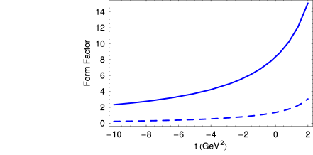
Figure 4: Dependence of $F^{(1a)}_{\rm\pi D^{\ast}D}(t)$ (solid line) and $F^{(a)}_{\rm J/\psi D^{\ast}D}(t)$ (dashed line) on the invariant variable ‘t” which is the $D^{\ast}$-momentum squared.

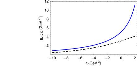
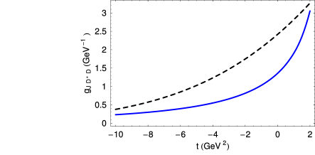
Figure 5: Comparison of our (solid line) form factors $F^{(1a)}_{\rm D\,J/\psi\,D}(t)$ and $F^{(a)}_{\rm J/\psi D^{\ast}D}(t)$ with those (dashed line) obtained in Matheus:2003pk .

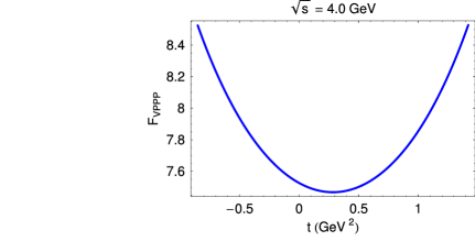
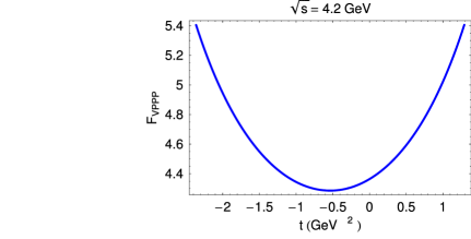
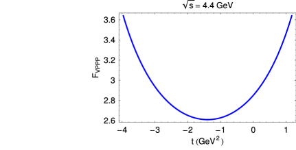
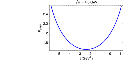
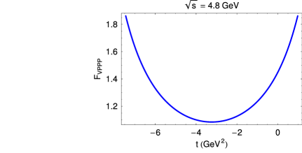
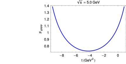
Figure 6: Dependence of the form factor $F_{\rm J/\psi\,\bar{D}\,\pi\,D}(s,t)$ on t for different values of $\sqrt{s}$.

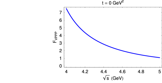
Figure 7: Dependence of the form factor $F_{\rm J/\psi\,\bar{D}\,\pi\,D}(s,t)$ on $s$ at $t=0$.

In Fig. 8 we separately plot the contributions coming from the box and resonance diagrams for the process $J/\psi+\pi^{+}\to D^{+}+\overline{D^{0}}$.

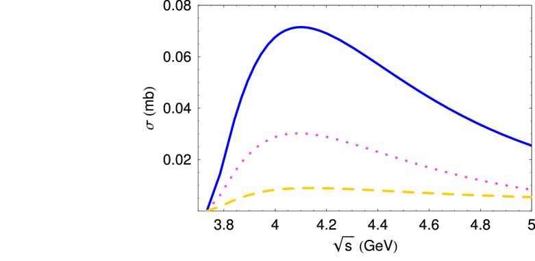
Figure 8: Contributions of the box (dotted curve) and resonance (dashed curve) diagrams to total (solid curve) cross section for the process $J/\psi+\pi^{+}\to D^{+}+\overline{D^{0}}$.

We display the dependence of the cross sections on the variable $\sqrt{s}$ for each channel in Fig. 9. The total cross section is a sum over all channels,

$$\sigma_{\rm tot}(s)=\sigma_{D^{+}\overline{D^{0}}}(s)+\sigma_{D^{\ast\,+}\overline{D^{0}}}(s)+\sigma_{D^{+}\overline{D^{\ast\,0}}}(s)+\sigma_{D^{\ast\,+}\overline{D^{\ast\,0}}}(s).$$ (27)

which are plotted in Fig. 9 Note that $\sigma_{D^{+}\overline{D^{\ast\,0}}}=\sigma_{D^{\ast\,+}\overline{D^{0}}}$. We plot $\sigma_{\rm tot}(s)$ as a function of $\sqrt{s}$ in Fig. 10. One can see that the maximum is about 2.3 mb at $\sqrt{s}\approx 4.1$ GeV. This is close to the result obtained in Wong:1999zb ; Wong:2001td ; Barnes:2003dg .

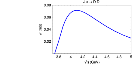
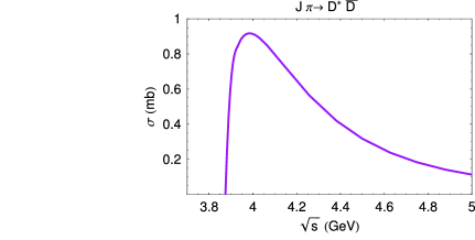
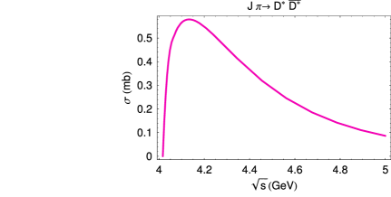
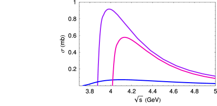
Figure 9: The cross sections of the processes $J/\psi+\pi^{+}\to D^{+}+\overline{D^{0}}$, $J/\psi+\pi^{+}\to D^{\ast\,+}+\overline{D^{0}}$ and $J/\psi+\pi^{+}\to D^{\ast\,+}+\overline{D^{\ast\,0}}$. All three curves are shown together in the last plot.

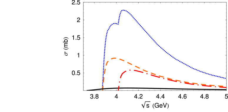
Figure 10: The total cross section (dotted line) together with the contributions already plotted in Fig. 9

Appendix A Expressions for form factors

Here we report the analytical expressions for the form factors involved in the calculation of the amplitudes $J/\psi+\pi^{+}\to D^{\ast\,+}+\overline{D^{\,0}}$ and $J/\psi+\pi^{+}\to D^{\ast\,+}+\overline{D^{\ast\,0}}$, respectively.

$J/\psi+\pi^{+}\to D^{\ast\,+}+\overline{D^{\,0}}$

$$F^{(i)}_{\rm VPPV}(s,t) = g_{J/\psi}\,g_{D}\,g_{D^{\ast}}\,g_{\pi}\int\!d\sigma_{\Box}\cdot\exp(-w\cdot z_{\Box}(s,t))\cdot N_{\rm VPPV}^{(i)}$$

$$N_{\rm VPPV}^{(1)} = -m_{q}\,m_{c}\,w^{2}+m_{q}^{2}\,w^{2}\,(2\,d_{1}\,d_{3}-2\,d_{2}\,d_{3}-d_{3})+m_{c}^{2}\,w^{2}\,(-1+d_{1}-d_{2})$$

$$+m^{2}_{J/\psi}\,w^{2}\,(-4\,d_{1}\,d_{2}\,d_{3}-2\,d_{1}\,d_{2}\,d_{3}^{2}-2\,d_{1}\,d_{2}-2\,d_{1}\,d_{2}^{2}\,d_{3}$$

$$-d_{1}\,d_{2}^{2}-2\,d_{1}\,d_{3}-d_{1}\,d_{3}^{2}-d_{1}$$

$$+4\,d_{1}^{2}\,d_{2}\,d_{3}+2\,d_{1}^{2}\,d_{2}+4\,d_{1}^{2}\,d_{3}$$

$$+2\,d_{1}^{2}\,d_{3}^{2}+2\,d_{1}^{2}-2\,d_{1}^{3}\,d_{3}-d_{1}^{3})$$

$$+m^{2}_{D}\,w^{2}\,(-6\,d_{1}\,d_{2}\,d_{3}+2\,d_{1}\,d_{2}\,d_{3}^{2}-2\,d_{1}\,d_{2}-4\,d_{1}\,d_{2}^{2}\,d_{3}-2\,d_{1}\,d_{2}^{2}-2\,d_{1}\,d_{3}$$

$$+2\,d_{1}\,d_{3}^{2}+2\,d_{1}^{2}\,d_{2}\,d_{3}+d_{1}^{2}\,d_{2}+2\,d_{1}^{2}\,d_{3}$$

$$+2\,d_{2}\,d_{3}-3\,d_{2}\,d_{3}^{2}+d_{2}+4\,d_{2}^{2}\,d_{3}-2\,d_{2}^{2}\,d_{3}^{2}+2\,d_{2}^{2}+2\,d_{2}^{3}\,d_{3}+d_{2}^{3}-d_{3}^{2})$$

$$+m^{2}_{D}\,w^{2}\,(-2\,d_{1}\,d_{3}^{3}+d_{1}^{2}\,d_{3}+2\,d_{1}^{2}\,d_{3}^{2}-2\,d_{2}\,d_{3}$$

$$-2\,d_{2}\,d_{3}^{2}+2\,d_{2}\,d_{3}^{3}-d_{2}^{2}\,d_{3}-2\,d_{2}^{2}\,d_{3}^{2}-d_{3}-d_{3}^{2}+d_{3}^{3})$$

$$+u\,w^{2}\,(3\,d_{1}\,d_{2}\,d_{3}+2\,d_{1}\,d_{2}+2\,d_{1}\,d_{2}^{2}\,d_{3}+d_{1}\,d_{2}^{2}+d_{1}\,d_{3}-2\,d_{1}^{2}\,d_{2}\,d_{3}-d_{1}^{2}\,d_{2}-2\,d_{1}^{2}\,d_{3})$$

$$+s\,w^{2}\,(d_{1}\,d_{2}\,d_{3}+2\,d_{1}\,d_{2}\,d_{3}^{2}+d_{1}\,d_{3}+d_{1}\,d_{3}^{2}-d_{1}^{2}\,d_{3}-2\,d_{1}^{2}\,d_{3}^{2})$$

$$+t\,w^{2}\,(-d_{1}\,d_{2}\,d_{3}-2\,d_{1}\,d_{2}\,d_{3}^{2}-d_{1}\,d_{3}-2\,d_{1}\,d_{3}^{2}+2\,d_{2}\,d_{3}$$

$$+3\,d_{2}\,d_{3}^{2}+d_{2}^{2}\,d_{3}+2\,d_{2}^{2}\,d_{3}^{2}+d_{3}+d_{3}^{2})$$

$$+w\,(-3-8\,v\,d_{1}\,d_{3}-3\,v\,d_{1}+8\,v\,d_{2}\,d_{3}+3\,v\,d_{2}+5\,v\,d_{3}$$

$$+3\,v+8\,d_{1}\,d_{3}+3\,d_{1}-8\,d_{2}\,d_{3}-3\,d_{2}-5\,d_{3}),$$

$$N_{\rm VPPV}^{(2)} = +m_{q}^{2}\,w^{2}\,(-2\,d_{1}\,d_{2}+d_{2}+2\,d_{2}^{2})$$

$$+m^{2}_{J/\psi}\,w^{2}\,(d_{1}\,d_{2}\,d_{3}+2\,d_{1}\,d_{2}^{2}\,d_{3}+3\,d_{1}\,d_{2}^{2}+2\,d_{1}\,d_{2}^{3}-2\,d_{1}^{2}\,$$

$$d_{2}\,d_{3}-3\,d_{1}^{2}\,d_{2}-4\,d_{1}^{2}\,d_{2}^{2}+2\,d_{1}^{3}\,d_{2})$$

$$+m^{2}_{D}\,w^{2}\,(-2\,d_{1}\,d_{2}\,d_{3}+2\,d_{1}\,d_{2}-2\,d_{1}\,d_{2}^{2}\,d_{3}+7\,d_{1}\,d_{2}^{2}$$

$$+4\,d_{1}\,d_{2}^{3}-2\,d_{1}^{2}\,d_{2}-2\,d_{1}^{2}\,d_{2}^{2}+d_{2}\,d_{3}-d_{2}+3\,d_{2}^{2}\,d_{3}-4\,d_{2}^{2}+2\,d_{2}^{3}\,d_{3}-5\,d_{2}^{3}-2\,d_{2}^{4})$$

$$+m^{2}_{\pi}\,w^{2}\,(-d_{1}\,d_{2}\,d_{3}+2\,d_{1}\,d_{2}\,d_{3}^{2}-2\,d_{1}\,d_{2}-2\,d_{1}^{2}\,d_{2}\,d_{3}$$

$$+3\,d_{2}\,d_{3}-d_{2}\,d_{3}^{2}+3\,d_{2}^{2}\,d_{3}-2\,d_{2}^{2}\,d_{3}^{2}+2\,d_{2}^{3}\,d_{3}+d_{3})$$

$$+u\,w^{2}\,(-d_{1}\,d_{2}-3\,d_{1}\,d_{2}^{2}-2\,d_{1}\,d_{2}^{3}+2\,d_{1}^{2}\,d_{2}+2\,d_{1}^{2}\,d_{2}^{2})$$

$$+s\,w^{2}\,(-d_{1}\,d_{2}\,d_{3}+d_{1}\,d_{2}-2\,d_{1}\,d_{2}^{2}\,d_{3}+2\,d_{1}^{2}\,d_{2}\,d_{3})$$

$$+t\,w^{2}\,(2\,d_{1}\,d_{2}\,d_{3}+d_{1}\,d_{2}+2\,d_{1}\,d_{2}^{2}\,d_{3}$$

$$-d_{2}\,d_{3}-3\,d_{2}^{2}\,d_{3}-2\,d_{2}^{3}\,d_{3})$$

$$+w\,(1+8\,v\,d_{1}\,d_{2}+2\,v\,d_{1}-7\,v\,d_{2}-8\,v\,d_{2}^{2}-v-8\,d_{1}\,d_{2}-2\,d_{1}+7\,d_{2}+8\,d_{2}^{2}),$$

$$N_{\rm VPPV}^{(3)} = +m_{q}\,m_{c}\,w^{2}\,(2\,d_{3})+m_{q}^{2}\,w^{2}\,(-2\,d_{2}\,d_{3}+2\,d_{3}^{2})+m_{c}^{2}\,w^{2}\,(-1-d_{2})$$

$$+m^{2}_{J/\psi}\,w^{2}\,(-d_{1}\,d_{2}\,d_{3}-d_{1}\,d_{2}-2\,d_{1}\,d_{2}^{2}\,d_{3}-d_{1}\,d_{2}^{2}+d_{1}\,d_{3}$$

$$+4\,d_{1}\,d_{3}^{2}+2\,d_{1}\,d_{3}^{3}-d_{1}+2\,d_{1}^{2}\,d_{2}\,d_{3}+d_{1}^{2}\,d_{2}-2\,d_{1}^{2}\,d_{3}-2\,d_{1}^{2}\,d_{3}^{2}+d_{1}^{2})$$

$$+m^{2}_{D}\,w^{2}\,(2\,d_{1}\,d_{2}\,d_{3}^{2}-d_{1}\,d_{2}-2\,d_{1}\,d_{2}^{2}\,d_{3}$$

$$-d_{1}\,d_{2}^{2}+d_{1}\,d_{3}+2\,d_{1}\,d_{3}^{2}-d_{2}\,d_{3}-4\,d_{2}\,d_{3}^{2}$$

$$+2\,d_{2}\,d_{3}^{3}+d_{2}^{2}\,d_{3}-4\,d_{2}^{2}\,d_{3}^{2}+d_{2}^{2}+2\,d_{2}^{3}\,d_{3}+d_{2}^{3}+2\,d_{3}^{3})$$

$$+m^{2}_{\pi}\,w^{2}\,(-d_{1}\,d_{2}\,d_{3}-2\,d_{1}\,d_{2}\,d_{3}^{2}+2\,d_{1}\,d_{3}^{2}+2\,d_{1}\,d_{3}^{3}-d_{2}\,d_{3}$$

$$+d_{2}\,d_{3}^{2}+4\,d_{2}\,d_{3}^{3}-d_{2}^{2}\,d_{3}-2\,d_{2}^{2}\,d_{3}^{2}+d_{3}^{2}-2\,d_{3}^{4})$$

$$+u\,w^{2}\,(-2\,d_{1}\,d_{2}\,d_{3}^{2}+d_{1}\,d_{2}+2\,d_{1}\,d_{2}^{2}\,d_{3}+d_{1}\,d_{2}^{2}-d_{1}\,d_{3}-2\,d_{1}\,d_{3}^{2})$$

$$+s\,w^{2}\,(d_{1}\,d_{2}\,d_{3}+2\,d_{1}\,d_{2}\,d_{3}^{2}-2\,d_{1}\,d_{3}^{2}-2\,d_{1}\,d_{3}^{3})$$

$$+t\,w^{2}\,(d_{2}\,d_{3}-2\,d_{2}\,d_{3}^{3}+d_{2}^{2}\,d_{3}+2\,d_{2}^{2}\,d_{3}^{2}-2\,d_{3}^{2}-2\,d_{3}^{3})$$

$$+w\,(-1+8\,v\,d_{2}\,d_{3}+3\,v\,d_{2}-4\,v\,d_{3}-8\,v\,d_{3}^{2}+v-8\,d_{2}\,d_{3}-3\,d_{2}+4\,d_{3}+8\,d_{3}^{2}),$$

$$N_{\rm VPPV}^{(4)} = +m_{q}\,m_{c}\,w^{2}\,(-2\,d_{2})+m_{q}^{2}\,w^{2}\,(-2\,d_{2}\,d_{3}+2\,d_{2}^{2})+m_{c}^{2}\,w^{2}\,(1+d_{2})$$

$$+m^{2}_{J/\psi}\,w^{2}\,(-3\,d_{1}\,d_{2}\,d_{3}-2\,d_{1}\,d_{2}\,d_{3}^{2}-d_{1}\,d_{2}+d_{1}\,d_{2}^{2}$$

$$+2\,d_{1}\,d_{2}^{3}+d_{1}\,d_{3}+d_{1}+2\,d_{1}^{2}\,d_{2}\,d_{3}+d_{1}^{2}\,d_{2}-2\,d_{1}^{2}\,d_{2}^{2}-d_{1}^{2})$$

$$+m^{2}_{D}\,w^{2}\,(-2\,d_{1}\,d_{2}\,d_{3}-2\,d_{1}\,d_{2}^{2}\,d_{3}+d_{1}\,d_{2}^{2}+2\,d_{1}\,d_{2}^{3}+d_{2}\,d_{3}-2\,d_{2}\,d_{3}^{2}+5\,d_{2}^{2}\,d_{3}$$

$$-2\,d_{2}^{2}\,d_{3}^{2}-d_{2}^{2}+4\,d_{2}^{3}\,d_{3}-3\,d_{2}^{3}-2\,d_{2}^{4})$$

$$+m^{2}_{\pi}\,w^{2}\,(-d_{1}\,d_{2}\,d_{3}-2\,d_{1}\,d_{2}\,d_{3}^{2}-d_{1}\,d_{2}+2\,d_{1}\,d_{2}^{2}\,d_{3}+d_{1}\,d_{3}$$

$$+d_{2}\,d_{3}-d_{2}\,d_{3}^{2}+2\,d_{2}\,d_{3}^{3}+d_{2}^{2}\,d_{3}-4\,d_{2}^{2}\,d_{3}^{2}+2\,d_{2}^{3}\,d_{3}-d_{3}^{2})$$

$$+u\,w^{2}\,(2\,d_{1}\,d_{2}\,d_{3}+2\,d_{1}\,d_{2}^{2}\,d_{3}-d_{1}\,d_{2}^{2}-2\,d_{1}\,d_{2}^{3})$$

$$+s\,w^{2}\,(d_{1}\,d_{2}\,d_{3}+2\,d_{1}\,d_{2}\,d_{3}^{2}+d_{1}\,d_{2}-2\,d_{1}\,d_{2}^{2}\,d_{3}-d_{1}\,d_{3})$$

$$+t\,w^{2}\,(d_{2}\,d_{3}+2\,d_{2}\,d_{3}^{2}-d_{2}^{2}\,d_{3}+2\,d_{2}^{2}\,d_{3}^{2}-2\,d_{2}^{3}\,d_{3})$$

$$+w\,(1+8\,v\,d_{2}\,d_{3}-v\,d_{2}-8\,v\,d_{2}^{2}+2\,v\,d_{3}-v-8\,d_{2}\,d_{3}+d_{2}+8\,d_{2}^{2}-2\,d_{3}),$$

$$N_{\rm VPPV}^{(5)} = +m_{q}\,m_{c}\,m^{2}_{J/\psi}\,w^{2}\,(-1/2)+m_{q}\,m_{c}\,m^{2}_{\pi}\,w^{2}\,(-1/2)$$

$$+m_{q}\,m_{c}\,s\,w^{2}\,(1/2)+m_{q}^{2}\,m_{c}^{2}\,w^{2}\,(1)$$

$$+m_{q}^{2}\,m^{2}_{J/\psi}\,w^{2}\,(d_{1}\,d_{2}+d_{1}\,d_{3}+d_{1}-d_{1}^{2}-1/2\,d_{2}-1/2\,d_{3})$$

$$+m_{q}^{2}\,m^{2}_{D}\,w^{2}\,(d_{1}\,d_{2}+d_{2}\,d_{3}-1/2\,d_{2}-d_{2}^{2})$$

$$+m_{q}^{2}\,m^{2}_{\pi}\,w^{2}\,(d_{1}\,d_{3}+d_{2}\,d_{3}-1/2\,d_{3}-d_{3}^{2})$$

$$+m_{q}^{2}\,u\,w^{2}\,(-d_{1}\,d_{2}+1/2\,d_{2})$$

$$+m_{q}^{2}\,s\,w^{2}\,(-d_{1}\,d_{3}+1/2\,d_{3})$$

$$+m_{q}^{2}\,t\,w^{2}\,(-d_{2}\,d_{3})$$

$$+m_{q}^{2}\,w\,(1-v)$$

$$+m_{c}^{2}\,m^{2}_{J/\psi}\,w^{2}\,(d_{1}\,d_{2}+d_{1}\,d_{3}+3/2\,d_{1}-d_{1}^{2})$$

$$+m_{c}^{2}\,m^{2}_{D}\,w^{2}\,(-1/2+d_{1}\,d_{2}+d_{1}+d_{2}\,d_{3}-3/2\,d_{2}-d_{2}^{2}+d_{3})$$

$$+m_{c}^{2}\,m^{2}_{\pi}\,w^{2}\,(1/2+d_{1}\,d_{3}+1/2\,d_{1}+d_{2}\,d_{3}+1/2\,d_{2}-d_{3}^{2})$$

$$+m_{c}^{2}\,u\,w^{2}\,(-d_{1}\,d_{2}-d_{1})$$

$$+m_{c}^{2}\,s\,w^{2}\,(-d_{1}\,d_{3}-1/2\,d_{1})$$

$$+m_{c}^{2}\,t\,w^{2}\,(-1/2-d_{2}\,d_{3}-1/2\,d_{2}-d_{3})$$

$$+m_{c}^{2}\,w\,(2-2\,v)$$

$$+m^{2}_{J/\psi}\,m^{2}_{D}\,w^{2}\,(d_{1}\,d_{2}\,d_{3}+2\,d_{1}\,d_{2}\,d_{3}^{2}-4\,d_{1}\,d_{2}-5\,d_{1}\,d_{2}^{2}$$

$$-2\,d_{1}\,d_{2}^{3}+d_{1}\,d_{3}^{2}-1/2\,d_{1}+11/2\,d_{1}^{2}\,d_{2}+4\,d_{1}^{2}\,d_{2}^{2}+3/2\,d_{1}^{2}$$

$$-2\,d_{1}^{3}\,d_{2}-d_{1}^{3}-1/2\,d_{2}\,d_{3}^{2}+d_{2}+3/2\,d_{2}^{2}+1/2\,d_{2}^{3}-1/2\,d_{3}^{2})$$

$$+m^{2}_{J/\psi}\,m^{2}_{\pi}\,w^{2}\,(2\,d_{1}\,d_{2}\,d_{3}+2\,d_{1}\,d_{2}^{2}\,d_{3}+1/2\,d_{1}\,d_{2}^{2}-7/2\,d_{1}\,d_{3}^{2}$$

$$-2\,d_{1}\,d_{3}^{3}+1/2\,d_{1}+7/2\,d_{1}^{2}\,d_{3}+4\,d_{1}^{2}\,d_{3}^{2}-2\,d_{1}^{3}\,d_{3}-1/2\,d_{1}^{3}-d_{2}\,d_{3}-1/2\,d_{2}^{2}\,d_{3}-d_{3}+1/2\,d_{3}^{3})$$

$$+m^{2}_{J/\psi}\,u\,w^{2}\,(d_{1}\,d_{2}\,d_{3}+3/2\,d_{1}\,d_{2}+d_{1}\,d_{2}^{2}+1/2\,d_{1}\,d_{3}-2\,d_{1}^{2}\,d_{2}\,d_{3}$$

$$-4\,d_{1}^{2}\,d_{2}-2\,d_{1}^{2}\,d_{2}^{2}-d_{1}^{2}\,d_{3}-d_{1}^{2}+2\,d_{1}^{3}\,d_{2}+d_{1}^{3})$$

$$+m^{2}_{J/\psi}\,s\,w^{2}\,(d_{1}\,d_{2}\,d_{3}+1/2\,d_{1}\,d_{2}+3/2\,d_{1}\,d_{3}+d_{1}\,d_{3}^{2}$$

$$-2\,d_{1}^{2}\,d_{2}\,d_{3}-1/2\,d_{1}^{2}\,d_{2}-7/2\,d_{1}^{2}\,d_{3}-2\,d_{1}^{2}\,d_{3}^{2}-1/2\,d_{1}^{2}+2\,d_{1}^{3}\,d_{3}+1/2\,d_{1}^{3})$$

$$+m^{2}_{J/\psi}\,t\,w^{2}\,(-4\,d_{1}\,d_{2}\,d_{3}-2\,d_{1}\,d_{2}\,d_{3}^{2}-1/2\,d_{1}\,d_{2}-2\,d_{1}\,d_{2}^{2}\,d_{3}$$

$$-1/2\,d_{1}\,d_{2}^{2}-3/2\,d_{1}\,d_{3}-d_{1}\,d_{3}^{2}-1/2\,d_{1}+2\,d_{1}^{2}\,d_{2}\,d_{3}$$

$$+1/2\,d_{1}^{2}\,d_{2}+d_{1}^{2}\,d_{3}+1/2\,d_{1}^{2}+d_{2}\,d_{3}+1/2\,d_{2}\,d_{3}^{2}+1/2\,d_{2}^{2}\,d_{3}+1/2\,d_{3}+1/2\,d_{3}^{2})$$

$$+m^{2}_{J/\psi}\,w\,(-3/2-5\,v\,d_{1}\,d_{2}-5\,v\,d_{1}\,d_{3}-13/2\,v\,d_{1}+5\,v\,d_{1}^{2}$$

$$+3/2\,v\,d_{2}+3/2\,v\,d_{3}+3/2\,v+5\,d_{1}\,d_{2}+5\,d_{1}\,d_{3}+13/2\,d_{1}-5\,d_{1}^{2}-3/2\,d_{2}-3/2\,d_{3})$$

$$+m^{4}_{J/\psi}\,w^{2}\,(-d_{1}\,d_{2}\,d_{3}-d_{1}\,d_{2}-1/2\,d_{1}\,d_{2}^{2}-d_{1}\,d_{3}-1/2\,d_{1}\,d_{3}^{2}$$

$$+2\,d_{1}^{2}\,d_{2}\,d_{3}+3\,d_{1}^{2}\,d_{2}+d_{1}^{2}\,d_{2}^{2}+3\,d_{1}^{2}\,d_{3}+d_{1}^{2}\,d_{3}^{2}$$

$$+3/2\,d_{1}^{2}-2\,d_{1}^{3}\,d_{2}-2\,d_{1}^{3}\,d_{3}-5/2\,d_{1}^{3}+d_{1}^{4})$$

$$+m^{2}_{D}\,m^{2}_{\pi}\,w^{2}\,(-d_{1}\,d_{2}\,d_{3}-d_{1}\,d_{3}+2\,d_{1}^{2}\,d_{2}\,d_{3}+1/2\,d_{1}^{2}\,d_{2}$$

$$+d_{1}^{2}\,d_{3}+5/2\,d_{2}\,d_{3}^{2}-2\,d_{2}\,d_{3}^{3}+1/2\,d_{2}-d_{2}^{2}\,d_{3}+4\,d_{2}^{2}\,d_{3}^{2}$$

$$-2\,d_{2}^{3}\,d_{3}-1/2\,d_{2}^{3}-1/2\,d_{3}-d_{3}^{3})$$

$$+m^{2}_{D}\,u\,w^{2}\,(-2\,d_{1}\,d_{2}\,d_{3}+3/2\,d_{1}\,d_{2}-2\,d_{1}\,d_{2}^{2}\,d_{3}$$

$$+7/2\,d_{1}\,d_{2}^{2}+2\,d_{1}\,d_{2}^{3}-2\,d_{1}^{2}\,d_{2}-2\,d_{1}^{2}\,d_{2}^{2}+1/2\,d_{2}\,d_{3}-1/2\,d_{2}$$

$$+1/2\,d_{2}^{2}\,d_{3}-d_{2}^{2}-1/2\,d_{2}^{3})$$

$$+m^{2}_{D}\,s\,w^{2}\,(2\,d_{1}\,d_{2}\,d_{3}-2\,d_{1}\,d_{2}\,d_{3}^{2}+1/2\,d_{1}\,d_{2}+2\,d_{1}\,d_{2}^{2}\,d_{3}$$

$$+1/2\,d_{1}\,d_{2}^{2}+d_{1}\,d_{3}-d_{1}\,d_{3}^{2}-2\,d_{1}^{2}\,d_{2}\,d_{3}-1/2\,d_{1}^{2}\,d_{2}-d_{1}^{2}\,d_{3}$$

$$-1/2\,d_{2}\,d_{3}+1/2\,d_{2}\,d_{3}^{2}-1/2\,d_{2}-1/2\,d_{2}^{2}\,d_{3}-1/2\,d_{2}^{2}+1/2\,d_{3}^{2})$$

$$+m^{2}_{D}\,t\,w^{2}\,(-2\,d_{1}\,d_{2}\,d_{3}-1/2\,d_{1}\,d_{2}-2\,d_{1}\,d_{2}^{2}\,d_{3}$$

$$-1/2\,d_{1}\,d_{2}^{2}+1/2\,d_{2}\,d_{3}-2\,d_{2}\,d_{3}^{2}+5/2\,d_{2}^{2}\,d_{3}-2\,d_{2}^{2}\,d_{3}^{2}$$

$$+1/2\,d_{2}^{2}+2\,d_{2}^{3}\,d_{3}+1/2\,d_{2}^{3})$$

$$+m^{2}_{D}\,w\,(-1-5\,v\,d_{1}\,d_{2}-2\,v\,d_{1}-5\,v\,d_{2}\,d_{3}+4\,v\,d_{2}$$

$$+5\,v\,d_{2}^{2}-2\,v\,d_{3}+v+5\,d_{1}\,d_{2}+2\,d_{1}+5\,d_{2}\,d_{3}-4\,d_{2}-5\,d_{2}^{2}+2\,d_{3})$$

$$+m^{4}_{D}\,w^{2}\,(2\,d_{1}\,d_{2}\,d_{3}-d_{1}\,d_{2}+2\,d_{1}\,d_{2}^{2}\,d_{3}-3\,d_{1}\,d_{2}^{2}-2\,d_{1}\,d_{2}^{3}+d_{1}^{2}\,d_{2}+d_{1}^{2}\,d_{2}^{2}$$

$$-d_{2}\,d_{3}+d_{2}\,d_{3}^{2}+1/2\,d_{2}-3\,d_{2}^{2}\,d_{3}+d_{2}^{2}\,d_{3}^{2}+3/2\,d_{2}^{2}-2\,d_{2}^{3}\,d_{3}+2\,d_{2}^{3}+d_{2}^{4})$$

$$+m^{2}_{\pi}\,u\,w^{2}\,(2\,d_{1}\,d_{2}\,d_{3}^{2}-2\,d_{1}\,d_{2}^{2}\,d_{3}-1/2\,d_{1}\,d_{2}^{2}$$

$$+1/2\,d_{1}\,d_{3}+d_{1}\,d_{3}^{2}-2\,d_{1}^{2}\,d_{2}\,d_{3}-1/2\,d_{1}^{2}\,d_{2}-d_{1}^{2}\,d_{3}+1/2\,d_{2}\,d_{3}$$

$$-1/2\,d_{2}\,d_{3}^{2}+1/2\,d_{2}^{2}\,d_{3}+1/2\,d_{3})$$

$$+m^{2}_{\pi}\,s\,w^{2}\,(-d_{1}\,d_{2}\,d_{3}-2\,d_{1}\,d_{2}\,d_{3}^{2}+1/2\,d_{1}\,d_{3}$$

$$+3/2\,d_{1}\,d_{3}^{2}+2\,d_{1}\,d_{3}^{3}-d_{1}^{2}\,d_{3}-2\,d_{1}^{2}\,d_{3}^{2}+1/2\,d_{2}\,d_{3}+1/2\,d_{2}\,d_{3}^{2}+1/2\,d_{3}-1/2\,d_{3}^{3})$$

$$+m^{2}_{\pi}\,t\,w^{2}\,(-d_{1}\,d_{2}\,d_{3}-2\,d_{1}\,d_{2}\,d_{3}^{2}-1/2\,d_{1}\,d_{3}-d_{1}\,d_{3}^{2}$$

$$-1/2\,d_{2}\,d_{3}+2\,d_{2}\,d_{3}^{3}-d_{2}^{2}\,d_{3}-2\,d_{2}^{2}\,d_{3}^{2}+1/2\,d_{3}+d_{3}^{2}+d_{3}^{3})$$

$$+m^{2}_{\pi}\,w\,(-1/2-5\,v\,d_{1}\,d_{3}-3/2\,v\,d_{1}-5\,v\,d_{2}\,d_{3}-3/2\,v\,d_{2}$$

$$+5/2\,v\,d_{3}+5\,v\,d_{3}^{2}+1/2\,v+5\,d_{1}\,d_{3}$$

$$+3/2\,d_{1}+5\,d_{2}\,d_{3}+3/2\,d_{2}-5/2\,d_{3}-5\,d_{3}^{2})$$

$$+m^{4}_{\pi}\,w^{2}\,(d_{1}\,d_{2}\,d_{3}+2\,d_{1}\,d_{2}\,d_{3}^{2}-d_{1}\,d_{3}^{2}-2\,d_{1}\,d_{3}^{3}+1/2\,d_{1}^{2}\,d_{3}$$

$$+d_{1}^{2}\,d_{3}^{2}-d_{2}\,d_{3}^{2}-2\,d_{2}\,d_{3}^{3}+1/2\,d_{2}^{2}\,d_{3}+d_{2}^{2}\,d_{3}^{2}-1/2\,d_{3}-1/2\,d_{3}^{2}+1/2\,d_{3}^{3}+d_{3}^{4})$$

$$+u\,s\,w^{2}\,(-d_{1}\,d_{2}\,d_{3}-1/2\,d_{1}\,d_{2}-1/2\,d_{1}\,d_{3}+2\,d_{1}^{2}\,d_{2}\,d_{3}+1/2\,d_{1}^{2}\,d_{2}+d_{1}^{2}\,d_{3})$$

$$+u\,t\,w^{2}\,(2\,d_{1}\,d_{2}\,d_{3}+1/2\,d_{1}\,d_{2}+2\,d_{1}\,d_{2}^{2}\,d_{3}+1/2\,d_{1}\,d_{2}^{2}-1/2\,d_{2}\,d_{3}-1/2\,d_{2}^{2}\,d_{3})$$

$$+u\,w\,(1/2+5\,v\,d_{1}\,d_{2}+2\,v\,d_{1}-3/2\,v\,d_{2}-1/2\,v-5\,d_{1}\,d_{2}-2\,d_{1}+3/2\,d_{2})$$

$$+u^{2}\,w^{2}\,(-1/2\,d_{1}\,d_{2}-1/2\,d_{1}\,d_{2}^{2}+d_{1}^{2}\,d_{2}+d_{1}^{2}\,d_{2}^{2})$$

$$+s\,t\,w^{2}\,(d_{1}\,d_{2}\,d_{3}+2\,d_{1}\,d_{2}\,d_{3}^{2}+1/2\,d_{1}\,d_{3}+d_{1}\,d_{3}^{2}-1/2\,d_{2}\,d_{3}-1/2\,d_{2}\,d_{3}^{2}-1/2\,d_{3}-1/2\,d_{3}^{2})$$

$$+s\,w\,(1+5\,v\,d_{1}\,d_{3}+3/2\,v\,d_{1}-3/2\,v\,d_{3}-v-5\,d_{1}\,d_{3}-3/2\,d_{1}+3/2\,d_{3})$$

$$+s^{2}\,w^{2}\,(-1/2\,d_{1}\,d_{3}-1/2\,d_{1}\,d_{3}^{2}+1/2\,d_{1}^{2}\,d_{3}+d_{1}^{2}\,d_{3}^{2})$$

$$+t\,w\,(-1/2+5\,v\,d_{2}\,d_{3}+3/2\,v\,d_{2}+2\,v\,d_{3}+1/2\,v-5\,d_{2}\,d_{3}-3/2\,d_{2}-2\,d_{3})$$

$$+t^{2}\,w^{2}\,(1/2\,d_{2}\,d_{3}+d_{2}\,d_{3}^{2}+1/2\,d_{2}^{2}\,d_{3}+d_{2}^{2}\,d_{3}^{2})$$

$$+3-6\,v+3\,v^{2};$$

$$F^{(1a)}_{\rm PVP}(t) = g_{\pi}\,g_{D^{\ast}}\,g_{D}\,\int\!d\sigma_{\triangle}\cdot\exp(-wz_{\triangle}(t))\,\cdot[w\,m_{q}\,m_{c}\,(-1)+w\,m_{q}^{2}\,(-b_{1})$$

$$+w\,m^{2}_{\pi}\,(b_{1}^{2}\,b_{2}-b_{1}^{2}+b_{1}^{3})+w\,t\,(b_{1}\,b_{2}^{2}+b_{1}^{2}\,b_{2}-b_{2}+b_{2}^{2})$$

$$+w\,m^{2}_{D}\,(-b_{1}^{2}\,b_{2})+v\,(1+3\,b_{1})-1-3\,b_{1}],$$

$$F^{(2a)}_{\rm PVP}(t) = g_{J/\psi}\,g_{D^{\ast}}\,g_{D}\,\int\!d\sigma_{\triangle}\cdot\exp(-wz_{\triangle}(t))\,\cdot[w\,m_{q}^{2}\,(1-b_{2})$$

$$+w\,m^{2}_{\pi}\,(-3\,b_{1}\,b_{2}+b_{1}\,b_{2}^{2}+b_{1}+b_{1}^{2}\,b_{2}-b_{1}^{2}+b_{2}-b_{2}^{2})$$

$$+w\,t\,(-b_{1}\,b_{2}+b_{1}\,b_{2}^{2}+b_{2}-2\,b_{2}^{2}+b_{2}^{3})$$

$$+w\,m^{2}_{D}\,(b_{1}\,b_{2}-b_{1}\,b_{2}^{2}-b_{2}+b_{2}^{2})$$

$$+v\,(-2+3\,b_{2})+2-3\,b_{2}],$$

$$F^{(b)}_{\rm PVV}(u) = g_{\pi}\,g^{2}_{D^{\ast}}\int\!d\sigma_{\triangle}\cdot\exp(-wz_{\triangle}(u))\,\cdot[w\,(m_{q}\,(b_{2}-1)-m_{c}\,b_{2})],$$

$$F^{(b)}_{\rm VPV}(u) = g_{J/\psi}\,g_{D}\,g_{D^{\ast}}\,\int\!d\sigma_{\triangle}\cdot\exp(-wz_{\triangle}(u))\cdot[w\,(m_{c}\,(b_{2}-1)-m_{q}\,b_{2})],$$

$$F^{(c)}_{\rm PVP}(u) = g_{\pi}\,g_{D^{\ast}}\,g_{D}\,\int\!d\sigma_{\triangle}\cdot\exp(-wz_{\triangle}(u))\,\cdot[w\,((-m_{c}\,m_{q}-m_{q}^{2}\,b_{1})$$

$$+m^{2}_{\pi}\,b_{1}^{2}\,(b_{2}-1+b_{1})$$

$$+m^{2}_{D}\,b_{2}\,(b_{1}\,b_{2}+b_{1}^{2}-1+b_{2})$$

$$-u\,b_{1}^{2}\,b_{2})-(1-v)\,(1+3\,b_{1})],$$

$$F^{(c)}_{\rm VPP}(u) = g_{J/\psi}\,g_{D}^{2}\,\int\!d\sigma_{\triangle}\cdot\exp(-wz_{\triangle}(u))\,\cdot[w\,(-2\,m_{c}\,m_{q}\,b_{2}+m_{c}^{2}\,(-1+b_{2})$$

$$+m^{2}_{J/\psi}\,b_{1}\,(b_{2}^{2}-1+b_{1}\,b_{2}+b_{1})$$

$$+m^{2}_{D}\,b_{2}^{2}\,(b_{1}-1+b_{2})-u\,b_{1}\,b_{2}^{2})$$

$$-(1-v)\,(1+3\,b_{2})]$$

$J/\psi+\pi^{+}\to D^{\ast\,+}+\overline{D^{\ast\,0}}$

$$F^{(i)}_{\rm VVPV}(s,t) = g_{J/\psi}\,g^{2}_{D^{\ast}}\,g_{\pi}\int\!d\sigma_{\Box}\cdot\exp(-w\cdot z_{\Box}(s,t))\cdot N_{\rm VVPV}^{(i)}$$

$$N_{\rm VVPV}^{(1)} = -\,w^{2}m_{q}\,d_{2},$$

$$N_{\rm VVPV}^{(2)} = w^{2}m_{c}\,d_{1},$$

$$N_{\rm VVPV}^{(3)} = w^{2}m_{c}\,(1-d_{1}+d_{2}),$$

$$N_{\rm VVPV}^{(4)} = w^{2}m_{c}\,(1-2\,d_{1}+d_{2}),$$

$$N_{\rm VVPV}^{(5)} = -w^{2}m_{c}\,d_{1},$$

$$N_{\rm VVPV}^{(6)} = w^{2}\left(m_{c}\,(1-d_{1}+d_{2})-m_{q}\,d_{3}\right),$$

$$N_{\rm VVPV}^{(7)} = -w^{2}m_{q}\,d_{3},$$

$$N_{\rm VVPV}^{(8)} = w^{2}d_{3}\,\left(m_{q}\,(2\,d_{1}-1)-2\,m_{c}\,d_{1}\right),$$

$$N_{\rm VVPV}^{(9)} = w^{2}d_{2}\,\left(m_{q}\,(1-2\,d_{1})+2\,m_{c}\,d_{1}\right),$$

$$N_{\rm VVPV}^{(10)} = w^{2}(m_{q}\,d_{2}-m_{c}\,d_{1}),$$

$$N_{\rm VVPV}^{(11)} = w^{2}\left(m_{q}\,d_{2}+m_{c}\,(d_{1}-d_{2}-1)\right),$$

$$N_{\rm VVPV}^{(12)} = -w^{2}m_{c}\,d_{1},$$

$$N_{\rm VVPV}^{(13)} = w^{2}m_{c}\,(d_{1}-d_{2}-1),$$

$$N_{\rm VVPV}^{(14)} = 2\,w^{2}d_{3}\,\left(m_{q}\,d_{2}-m_{c}\,(1+d_{2})\right),$$

$$N_{\rm VVPV}^{(15)} = -\,2\,w^{2}d_{2}\,\left(m_{q}\,d_{2}-m_{c}\,(1+d_{2})\right),$$

$$N_{\rm VVPV}^{(16)} = w^{2}m_{c}\,\left\{-m_{q}^{2}+m_{J/\psi}^{2}\,d_{1}\,\left(d_{1}-\frac{3}{2}-d_{2}-d_{3}\right)\right.$$

$$+ m_{D^{\ast}}^{2}\,\left(\frac{1}{2}-d_{1}d_{2}-d_{1}-d_{2}d_{3}+\frac{3}{2}\,d_{2}+d_{2}^{2}-d_{3}\right)$$

$$+ m_{\pi}^{2}\,\left(-\frac{1}{2}-d_{1}d_{3}-\frac{1}{2}\,d_{1}-d_{2}d_{3}-\frac{1}{2}\,d_{2}+d_{3}^{2}\right)$$

$$+ \left.u\,d_{1}\,(1+d_{2})+(p_{1}+s\,d_{1}\,\left(\frac{1}{2}+d_{3}\right)+t\,\left(\frac{1}{2}\,(1+d_{2})+d_{3}\,(1+d_{2})\right)\right\}$$

$$- 2\,m_{c}\,w(1-v),$$

$$N_{\rm VVPV}^{(17)} = w^{2}\,m_{q}\,\left\{-\,m_{c}^{2}+m_{J/\psi}^{2}\,\left(-d_{1}d_{2}-d_{1}d_{3}-d_{1}+d_{1}^{2}+\frac{1}{2}\,(d_{2}+d_{3})\right)\right.$$

$$+ m_{D^{\ast}}^{2}\,d_{2}\,\left(d_{2}-d_{1}-d_{3}+\frac{1}{2}\right)+m_{\pi}^{2}\,d_{3}\,\left(d_{3}-d_{1}-d_{2}+\frac{1}{2}\right)$$

$$+ \left.u\,d_{2}\left(d_{1}-\frac{1}{2}\right)+s\,d_{3}\,\left(d_{1}-\frac{1}{2}\right)+t\,d_{2}\,d_{3}\right\}$$

$$- w\,(1-v)\,(m_{q}+m_{c}).$$

$$F^{(a)}_{\rm PVV}(t) = g_{\pi}\,g^{2}_{D^{\ast}}\,\int\!d\sigma_{\triangle}\cdot\exp(-wz_{\triangle}(t))\,\cdot[w\,(m_{q}\,(b_{2}-1)-m_{c}\,b_{2})],$$

$$F^{(1a)}_{\rm VVV}(t) = g_{J/\psi}\,g^{2}_{D^{\ast}}\,\int\!d\sigma_{\triangle}\cdot\exp(-wz_{\triangle}(t))\,\cdot[4\,w\,b_{1}\,b_{2}\,(b_{1}+b_{2}-1)],$$

$$F^{(2a)}_{\rm VVV}(t) = g_{J/\psi}\,g^{2}_{D^{\ast}}\,\int d\sigma_{\triangle}\cdot\exp(-wz_{\triangle}(t))\,\cdot[2\,w\,b_{2}\,(b_{1}-2\,b_{1}\,b_{2}-1+3\,b_{2}-2\,b_{2}^{2})],$$

$$F^{(3a)}_{\rm VVV}(t) = g_{J/\psi}\,g^{2}_{D^{\ast}}\,\int\!d\sigma_{\triangle}\cdot\exp(-wz_{\triangle}(t))\cdot[w\,(-m_{c}\,(m_{q}+m_{c}b_{1})+m^{2}_{J/\psi}\,b_{1}^{2}\,(b_{1}+b_{2}-1)$$

$$+ t\,b_{2}\,(b_{1}^{2}+b_{1}b_{2}+b_{2}-1)-m^{2}_{D}\,b_{1}^{2}\,b_{2})-(1-v)(b_{1}+1)],$$

$$F^{(4a)}_{\rm VVV}(t) = g_{J/\psi}\,g^{2}_{D^{\ast}}\,\int\!d\sigma_{\triangle}\cdot\exp(-wz_{\triangle}(t))\cdot[w\,(m_{c}^{2}(d2-1)+m^{2}_{J/\psi}\,(3\,b_{1}\,b_{2}-b_{1}\,b_{2}^{2}-b_{1}-b_{1}^{2}\,b_{2}+b_{1}^{2}-b_{2}+b_{2}^{2})$$

$$+ t\,(b_{1}\,b_{2}-b_{1}\,b_{2}^{2}-b_{2}+2\,b_{2}^{2}-b_{2}^{3})-m^{2}_{D}\,(b_{1}\,b_{2}+b_{1}\,b_{2}^{2}+b_{2}-b_{2}^{2}))+(1-v)\,(b_{2}-1)],$$

$$F^{(5a)}_{\rm VVV}(t) = g_{J/\psi}\,g^{2}_{D^{\ast}}\,\int\!d\sigma_{\triangle}\cdot\exp(-wz_{\triangle}(t))\cdot[w\,(m_{c}\,(m_{q}-m_{c}b_{1}-m_{c}b_{2}+m_{c})$$

$$+ m^{2}_{J/\psi}\,b_{1}\,(-2\,b_{2}+b_{2}^{2}+1+2\,b_{1}\,b_{2}-2\,b_{1}+b_{1}^{2})$$

$$+ t\,b_{2}\,(-2\,b_{1}+2\,b_{1}\,b_{2}+b_{1}^{2}+1-2\,b_{2}+b_{2}^{2})+m^{2}_{D}\,b_{1}\,b_{2}\,(2-b_{2}-b_{1}))+(1-v)\,(2-b_{1}-b_{2})],$$

$$F^{(6a)}_{\rm VVV}(t) = g_{J/\psi}\,g^{2}_{D^{\ast}}\int\!d\sigma_{\triangle}\cdot\exp(-wz_{\triangle}(t))\cdot[w\,(m_{c}\,(2\,m_{q}\,b_{2}-m_{c}\,b_{2}+m_{c})+m^{2}_{J/\psi}\,b_{1}\,(-b_{2}^{2}+1-b_{1}\,b_{2}-b_{1})$$

$$+ t\,b_{2}\,(-b_{1}\,b_{2}+b_{2}-b_{2}^{2})+m^{2}_{D}\,b_{1}\,b_{2}^{2})+(1-v)\,(b_{2}+1)],$$

$$F^{(c)}_{\rm PPV}(t) = g_{\pi}\,g_{D}\,g_{D^{\ast}}\int\!d\sigma_{\triangle}\cdot\exp(-wz_{\triangle}(t))\,\cdot[w\,(m_{q}\,(m_{c}-m_{q}b_{1}-m_{q}b_{2}+m_{q})$$

$$+ m^{2}_{J/\psi}\,b_{1}\,(1-2b_{1}-2b_{2}+b_{2}^{2}+2b_{1}b_{2}+b_{1}^{2})$$

$$+ t\,b_{2}\,(1-2b_{1}-2b_{2}+b_{1}^{2}+2b_{1}b_{2}+b_{2}^{2})+m^{2}_{D}\,b_{1}\,b_{2}\,(2-b_{1}-b_{2}))+(1-v)\,(4-3\,b_{1}-3\,b_{2})]$$

$$F^{(c)}_{\rm VPV}(t) = g_{J/\psi}\,g_{D}\,g_{D^{\ast}}\,\int\!d\sigma_{\triangle}\cdot\exp(-wz_{\triangle}(t))\cdot[w\,(m_{c}-b_{2}\,(m_{c}-m_{q}))].$$

References

- (1) M. C. Abreu et al. [NA50 Collaboration], Nucl. Phys. A 698, 543 (2002). M. C. Abreu et al. [NA50 Collaboration], Phys. Lett. B 477, 28 (2000).
- (2) T. Barnes, arXiv:nucl-th/0306031.
- (3) K. Martins, D. Blaschke and E. Quack, Phys. Rev. C 51, 2723 (1995) [arXiv:hep-ph/9411302].
- (4) C. Y. Wong, E. S. Swanson and T. Barnes, Phys. Rev. C 62, 045201 (2000) [arXiv:hep-ph/9912431].
- (5) C. Y. Wong, E. S. Swanson and T. Barnes, Phys. Rev. C 65, 014903 (2002) [Erratum-ibid. C 66, 029901 (2002)] [arXiv:nucl-th/0106067].
- (6) T. Barnes, E. S. Swanson, C. Y. Wong and X. M. Xu, Phys. Rev. C 68, 014903 (2003) [arXiv:nucl-th/0302052].
- (7) S. G. Matinian and B. Muller, Phys. Rev. C 58, 2994 (1998) [arXiv:nucl-th/9806027].
- (8) K. L. Haglin, Phys. Rev. C 61, 031902 (2000) [arXiv:nucl-th/9907034].
- (9) K. Haglin and C. Gale, J. Phys. G 30, S375 (2004) [arXiv:hep-ph/0305174].
- (10) Z. W. Lin and C. M. Ko, Phys. Rev. C 62, 034903 (2000) [arXiv:nucl-th/9912046].
- (11) Y. Oh, T. Song and S. H. Lee, Phys. Rev. C 63, 034901 (2001) [arXiv:nucl-th/0010064].
- (12) Y. Oh, T. s. Song, S. H. Lee and C. Y. Wong, J. Korean Phys. Soc. 43, 1003 (2003) [arXiv:nucl-th/0205065].
- (13) V. V. Ivanov, Y. L. Kalinovsky, D. Blaschke and G. R. Burau, arXiv:hep-ph/0112354.
- (14) F. S. Navarra, M. Nielsen, R. S. Marques de Carvalho and G. Krein, Phys. Lett. B 529, 87 (2002) [arXiv:nucl-th/0105058].
- (15) F. S. Navarra, M. Nielsen and M. E. Bracco, Phys. Rev. D 65, 037502 (2002) [arXiv:hep-ph/0109188].
- (16) R. D. Matheus, F. S. Navarra, M. Nielsen and R. Rodrigues da Silva, Phys. Lett. B 541, 265 (2002) [arXiv:hep-ph/0206198].
- (17) F. O. Duraes, H. c. Kim, S. H. Lee, F. S. Navarra and M. Nielsen, Phys. Rev. C 68, 035208 (2003) [arXiv:nucl-th/0211092].
- (18) G. I. Lykasov and A. Y. Illarionov, arXiv:hep-ph/0305117.
- (19) A. Deandrea, G. Nardulli and A. D. Polosa, Phys. Rev. D 68, 034002 (2003) [arXiv:hep-ph/0302273].
- (20) D. B. Blaschke, G. R. G. Burau, M. A. Ivanov, Y. L. Kalinovsky and P. C. Tandy, arXiv:hep-ph/0002047.
-
(21)
M. A. Ivanov, M. P. Locher and V. E. Lyubovitskij, Few Body Syst. 21, 131 (1996)
[arXiv:hep-ph/9602372];
M. A. Ivanov and V. E. Lyubovitskij, Phys. Lett. B 408, 435 (1997) [arXiv:hep-ph/9705423]. -
(22)
S. Weinberg, Phys.Rev. 130, 776 (1963);
K. Hayashi et al., Fort. der Phys. 15, 625 (1967). - (23) M. A. Ivanov, Y. L. Kalinovsky and C. D. Roberts, Phys. Rev. D 60, 034018 (1999) [arXiv:nucl-th/9812063].
-
(24)
M. A. Ivanov and P. Santorelli,
Phys. Lett. B 456, 248 (1999),
[arXiv:hep-ph/9903446];
M. A. Ivanov, J. G. Körner and P. Santorelli, Phys. Rev. D 63, 074010 (2001), [arXiv:hep-ph/0007169];
A. Faessler, T. Gutsche, M. A. Ivanov, J. G. Körner and V. E. Lyubovitskij, Eur. Phys. J. directC 4, 18 (2002), [arXiv:hep-ph/0205287];
A. Faessler, T. Gutsche, M. A. Ivanov, V. E. Lyubovitskij and P. Wang, Phys. Rev. D 68, 014011 (2003) [arXiv:hep-ph/0304031]. - (25) G. V. Efimov and M. A. Ivanov, “The Quark Confinement Model Of Hadrons,” Bristol, UK: IOP (1993) 177 p; Int. J. Mod. Phys. A 4, 2031 (1989).
- (26) S. Mandelstam, Annals Phys. 19, 1 (1962).
- (27) C. D. Roberts and A. G. Williams, Prog. Part. Nucl. Phys. 33, 477 (1994) [arXiv:hep-ph/9403224].
- (28) K. Hagiwara et al. [Particle Data Group Collaboration], Phys. Rev. D 66, 010001 (2002).
- (29) S. Ryan, Nucl. Phys. B (Proc. Suppl.) 106, 86 (2002).
- (30) T. M. Aliev and O. Yilmaz, Nuovo Cim. A 105 (1992) 827. P. Colangelo, G. Nardulli and N. Paver, Z. Phys. C 57, 43 (1993); M. Chabab, Phys. Lett. B 325, 205 (1994); V. V. Kiselev, Int. J. Mod. Phys. A 11, 3689 (1996) [arXiv:hep-ph/9504313].
- (31) A. I. Davydychev, P. Osland and L. Saks, JHEP 0108, 050 (2001) [arXiv:hep-ph/0105072].
- (32) J. G. Körner and M. C. Mauser, arXiv:hep-ph/0306082.
- (33) S. Ahmed et al. [CLEO Collaboration], Phys. Rev. Lett. 87, 251801 (2001) [arXiv:hep-ex/0108013].
- (34) V. M. Belyaev, V. M. Braun, A. Khodjamirian and R. Ruckl, Phys. Rev. D 51, 6177 (1995) [arXiv:hep-ph/9410280]; A. Khodjamirian, R. Ruckl, S. Weinzierl and O. I. Yakovlev, Phys. Lett. B 457, 245 (1999) [arXiv:hep-ph/9903421].
- (35) R. D. Matheus, F. S. Navarra, M. Nielsen and R. R. da Silva, arXiv:hep-ph/0310280.