Probing the Radion-Higgs mixing at hadronic colliders

Abstract

In the Randall-Sundrum model, the radion-Higgs mixing is weakly suppressed by the effective electroweak scale. One of its novel features would be a sizable three-point vertex of $h_{\mu\nu}^{(n)}$-$h$-$\phi$. We explored the potential of the Fermilab Tevatron and the CERN LHC in probing the radion-Higgs mixing via the associated production of the radion with the Higgs boson. The observation of the rare decay of the KK gravitons into $h\phi$ is then the direct and exclusive signal of the radion-Higgs mixing. We also studied all the partial decay widths of the KK gravitons in the presence of the radion-Higgs mixing, and found that if the mixing parameter is of order one, the decay rate into a radion and a Higgs boson becomes as large as that into a Higgs boson pair, with the branching ratio of order $10^{-3}$.

I Introduction

The standard model (SM) has been extraordinarily successful in explaining all experimental data on the electroweak interactions of the gauge bosons and fermions up to now. However, the master piece of the SM, the Higgs boson, still awaits experimental discovery Higgs . Theoretical consideration of the triviality and the unitarity puts an upper bound of $(8\pi\sqrt{2}/3G_{F})^{1/2}\sim 1$ TeV trivial ; Duncan:1986vj on the Higgs boson mass. On the other hand, the direct search has put a lower mass limit of 114.4 GeV on the SM Higgs boson at the 95% C.L. higgs , while the indirect evidences from the electroweak precision data imply a light Higgs boson of order ${\mathcal{O}}(100)$ GeV lepew . In order to establish the Higgs mechanism for the electroweak symmetry breaking, one also requires to study in detail the Higgs boson interactions with the gauge bosons and fermions. Therefore, one of the primary goals of future collider experiments is directed toward the study of the Higgs boson.

The Higgs boson is also a clue to various models of new physics beyond the SM, as its mass receives radiative corrections very sensitive to the UV physics. This is the so-called gauge hierarchy problem. Recently, a lot of theoretical and phenomenological interests have been drawn to a scenario proposed by Randall and Sundrum (RS) RS , where an additional spatial dimension of a $S^{1}/Z_{2}$ orbifold is introduced with two 3-branes at the fixed points. A geometrical suppression factor, called the warp factor, emerges and naturally explains the huge hierarchy between the electroweak and Planck scale with moderate values of the model parameters. A stabilization mechanism was introduced GW to maintain the brane separation, and to avoid unconventional cosmological phenomenologies Csaki-cosmology . Such a mechanism introduces a radion much lighter than the Kaluza-Klein (KK) states of any bulk fields. In the literature, various phenomenological aspects of the radion have been studied such as its decay modes Ko ; Wells , its effects on the electroweak precision observations Csaki-EW , and its phenomenological signatures at present and future colliders collider .

In the viewpoint of the Higgs phenomenology, the presence of another scalar (the radion) may modify the characteristics of the Higgs boson itself even in the minimal RS scenario where all the SM fields are confined on the TeV brane. It is due to the radion-Higgs mixing originated from the gravity-scalar mixing term, $\xi R(g_{\rm vis})\widehat{H}^{\dagger}\widehat{H}$, where $R(g_{\rm vis})$ being the Ricci scalar of the induced metric $g_{\rm vis}^{\mu\nu}$. Here $\widehat{H}$ is the Higgs field in the five-dimensional context. It has been shown that the radion-Higgs mixing can induce significant deviations to the properties of the SM Higgs boson Datta-HR-LHC ; Han-unitarity ; Hewett:2002nk ; Gunion .

A complementary way to probe the radion-Higgs mixing is the direct search for the new couplings exclusively allowed with a non-zero mixing parameter $\xi$. One good example is the tri-linear vertex among the KK graviton, the Higgs boson, and the radion. In Ref. ours , we have shown that, especially in the limit of large VEV of the radion, probing the $h_{\mu\nu}^{(n)}$-$h$-$\phi$ through the $h\phi$ production at $e^{+}e^{-}$ colliders can provide very useful information on the radion-Higgs mixing, irrespective of the mass spectrum of the Higgs and radion. This high energy collision process is complementary to the rare decay modes of the Higgs boson allowed with non-zero $\xi$, $e.g.$, $h\to\phi\phi$ which can be sizable in some parameter space Gunion .

In this work, we focus on the associated production of the radion with the Higgs boson at hadronic colliders, the Fermilab Tevatron and the CERN Large Hadron Collider (LHC). The higher center-of-mass (c.m.) energy of the hadron colliders allows the on-shell production of KK gravitons, the decay of which in turn yields clean signals of the RS model. The observation of the rare decay of the KK gravitons into $h\phi$ is then the direct and exclusive signal of the radion-Higgs mixing. In addition, the characteristic angular distribution could reveal the exchange of massive spin-2 KK gravitons.

This paper is organized as follows. Section II summarizes the RS model and the basic properties of the radion-Higgs mixing. In Sec. III, we calculate the partial decay widths of the graviton in the presence of the radion-Higgs mixing. The production cross section of $p\,p\,(\bar{p})\to h\,\phi$ and the corresponding kinematic distributions are discussed in Sec. IV. Section V deals with the feasibility of detecting the $h\phi$ final states by considering specific decay channels of the Higgs and radion. We summarize and conclude in Sec. VI.

II Review of the Randall-Sundrum model and radion-Higgs mixing

The RS scenario is based on a five-dimensional spacetime with non-factorizable geometry RS . The single extra dimension is compactified on a $S^{1}/Z_{2}$ orbifold of which two fixed points accommodate two three-branes, the Planck brane at $y=0$ and the TeV brane at $y=1/2$. Four-dimensional Poincare invariance is shown to be maintained by the following classical solution to the Einstein equation:

$$ds^{2}=e^{-2\sigma(y)}\eta_{\mu\nu}dx^{\mu}dx^{\nu}-b_{0}^{2}dy^{2},$$ (1)

where $\eta_{\mu\nu}$ is the Minkowski metric, $\sigma(y)=m_{0}b_{0}|y|$, and $y\in[0,1/2]$. The five-dimensional Planck mass $M_{5}$ ($\epsilon\equiv 1/M_{5}^{3}$) is related to the four-dimensional Planck mass ($M_{\rm Pl}\equiv 1/\sqrt{8\pi G_{N}}$) by

$${M_{\rm Pl}^{2}\over 2}={1-\Omega_{0}^{2}\over\epsilon^{2}m_{0}},$$ (2)

where $\Omega_{0}\equiv e^{-m_{0}b_{0}/2}$ is the warp factor. On the TeV brane one observes the mass of a canonically normalized scalar field to be multiplied by the small warp factor, $i.e.$, $m_{phys}=\Omega_{0}m_{0}$. As the moderate value of $m_{0}b_{0}/2\simeq 35$ can generate TeV scale physical mass, the gauge hierarchy problem is answered.

In the minimal RS model, all the SM fields are confined on the TeV brane. Gravitational fluctuations about the RS metric such as

$$\eta_{\mu\nu}\to\eta_{\mu\nu}+\epsilon h_{\mu\nu}(x,y),\;\;\;\;\;\;b_{0}\to b_{0}+b(x)\,$$ (3)

yield two kinds of new phenomenological ingredients on the TeV brane, the KK graviton mode $h_{\mu\nu}^{(n)}(x)$ and the canonically normalized radion field $\phi_{0}(x)$, defined by

$$h_{\mu\nu}(x,y)=\sum_{n=0}^{\infty}h_{\mu\nu}^{(n)}(x)\frac{\chi^{(n)}(y)}{\sqrt{b_{0}}}\,,\quad\phi_{0}(x)=\sqrt{6}M_{\rm Pl}\Omega_{b}(x)\,,$$ (4)

where $\Omega_{b}(x)\equiv e^{-m_{0}[b_{0}+b(x)]/2}$. The four-dimensional effective Lagrangian is then

$${\cal L}=-\frac{\phi_{0}}{\Lambda_{\phi}}T_{\mu}^{\mu}-\frac{1}{\widehat{\Lambda}_{W}}T^{\mu\nu}(x)\sum_{n=1}^{\infty}h^{(n)}_{\mu\nu}(x)\,,$$ (5)

where $\Lambda_{\phi}(=\sqrt{6}M_{\rm Pl}\Omega_{0})$ is the vacuum expectation value (VEV) of the radion field, $T^{\mu}_{\mu}$ is the trace of the symmetric energy-momentum tensor $T^{\mu\nu}$, and $\widehat{\Lambda}_{W}=\sqrt{2}M_{\rm Pl}\Omega_{0}$. Note that both effective interactions are suppressed by the electroweak scale, not by the Planck scale.

All the SM symmetries and Poincare invariance on the TeV brane are still respected by the following gravity-scalar mixing term Wells ; Gunion :

$$S_{\xi}=\xi\int d^{4}x\sqrt{g_{\rm vis}}\,R(g_{\rm vis})\widehat{H}^{\dagger}\widehat{H}\,,$$ (6)

where $R(g_{\rm vis})$ is the Ricci scalar for the induced metric on the visible brane, $g^{\mu\nu}_{\rm vis}=\Omega_{b}^{2}(x)(\eta^{\mu\nu}+\epsilon h^{\mu\nu})$, $H_{0}=\Omega_{0}\widehat{H}$, and $\xi$ denotes the size of the mixing term. This $\xi$-term mixes the $h_{0}$ and $\phi_{0}$ fields into the mass eigenstates of $h$ and $\phi$ fields, given by Gunion

$$\left(\begin{array}[]{c}h_{0}\\ \phi_{0}\\ \end{array}\right)=\left(\begin{array}[]{cc}1&6\xi\gamma/Z\\ 0&-1/Z\\ \end{array}\right)\left(\begin{array}[]{rc}\cos\theta&\sin\theta\\ -\sin\theta&\cos\theta\\ \end{array}\right)\left(\begin{array}[]{c}h\\ \phi\\ \end{array}\right)=\left(\begin{array}[]{cc}d&c\\ b&a\\ \end{array}\right)\left(\begin{array}[]{c}h\\ \phi\\ \end{array}\right)\,,$$ (7)

where

$$Z^{2} \equiv 1+6\xi\gamma^{2}(1-6\xi)\equiv\beta-36\xi^{2}\gamma^{2}\,.$$ (8)

$$\tan 2\theta = 12\gamma\xi Z{m_{h_{0}}^{2}\over m_{\phi_{0}}^{2}-m_{h_{0}}^{2}(Z^{2}-36\xi^{2}\gamma^{2})}\,.$$ (9)

Note that in the RS scenario the radion-Higgs mixing is only suppressed by the electroweak scale of $1/\Lambda_{\phi}$.

The eigenvalues for the square of masses are

$$m_{\pm}^{2}={1\over 2Z^{2}}\left\{m_{\phi_{0}}^{2}+\beta m_{h_{0}}^{2}\pm\sqrt{(m_{\phi_{0}}^{2}+\beta m_{h_{0}}^{2})^{2}-4Z^{2}m_{\phi_{0}}^{2}m_{h_{0}}^{2}}\right\}\,,$$ (10)

where $m_{+}~{}(m_{-})$ is the larger (smaller) between the Higgs mass $m_{h}$ and the radion mass $m_{\phi}$. Our convention is that in the limit of $\xi\to 0$, $m_{h_{0}}$ is the Higgs mass. The following constraint on $\xi$ from the positivity of the mass squared in Eq. (10) is crucially operating in most of parameter space:

$${m_{+}^{2}\over m_{-}^{2}}>1+{2\beta\over Z^{2}}\left(1-{Z^{2}\over\beta}\right)+{2\beta\over Z^{2}}\left[1-{Z^{2}\over\beta}\right]^{1/2}\,.$$ (11)

All phenomenological signatures of the RS model including the radion-Higgs mixing are specified by five parameters

$$\xi,\quad\Lambda_{\phi},\quad\frac{m_{0}}{M_{\rm Pl}},\quad m_{\phi},\quad m_{h}\,,$$ (12)

which in turn determine $\widehat{\Lambda}_{W}={\Lambda_{\phi}}/\sqrt{3}$ and KK graviton masses $m_{G}^{(n)}=x_{n}{m_{0}}{\widehat{\Lambda}_{W}}/({M_{\rm Pl}}{\sqrt{2}})$ with $x_{n}$ being the $n$-th root of the first order Bessel function. Some comments on the parameters in Eq. (12) are in order. First, the dimensionless coefficient of the radion-Higgs mixing, $\xi$, is generally of order one with the constraint in Eq. (11). The $\Lambda_{\phi}$ which fixes the masses and effective couplings of KK gravitons is also constrained, $e.g.$, by the Tevatron Run I data of Drell-Yan process and by the electroweak precision data: $m_{G}^{(1)}\mathrel{\raise 1.29167pt\hbox{$>$\kern-7.5pt\lower 4.30554pt\hbox{$\sim$}}}600$ GeV yields $\Lambda_{\phi}\mathrel{\raise 1.29167pt\hbox{$>$\kern-7.5pt\lower 4.30554pt\hbox{$\sim$}}}4$ TeV RS-onoff . For the reliability of the RS solution, the ratio $m_{0}/M_{\rm Pl}$ is usually taken around $0.01\mathrel{\raise 1.29167pt\hbox{$<$\kern-7.5pt\lower 4.30554pt\hbox{$\sim$}}}m_{0}/M_{\rm Pl}\mathrel{\raise 1.29167pt\hbox{$<$\kern-7.5pt\lower 4.30554pt\hbox{$\sim$}}}0.1$ to avoid too large bulk curvature Hewett-bulk-gauge . Therefore, we consider the case of $\Lambda_{\phi}=5$ TeV and $m_{0}/M_{\rm Pl}=0.1$, where the effect of radion on the oblique parameters is small Csaki-EW . The radion mass is expected to be light as one of the simplest stabilization mechanisms predicts $m_{\phi_{0}}\sim\widehat{\Lambda}_{W}/40$ GW . In addition, the Higgs boson mass is set to be $120$ GeV through out the paper.

III Radion-Higgs mixing and Graviton Partial Decay Widths

The gravity-scalar mixing, $\xi\,R\,\widehat{H}^{\dagger}\widehat{H}$, modifies the couplings among the $h$, $\phi$ and $h_{\mu\nu}^{(n)}$. In particular, a non-zero $\xi$ newly generates the following tri-linear vertices:

$$h_{\mu\nu}^{(n)}\,\mbox{-}\,h\,\mbox{-}\,\phi,\quad h_{\mu\nu}^{(n)}\,\mbox{-}\,\phi\,\mbox{-}\,\phi,\quad h\,\mbox{-}\,\phi\,\mbox{-}\,\phi,\quad\phi\,\mbox{-}\,\phi\,\mbox{-}\,\phi\,.$$ (13)

Focused on the phenomenologies at hadron colliders, we are interested in the KK graviton production and its decay exclusively allowed to the radion-Higgs mixing through the vertices of $h_{\mu\nu}^{(n)}-h-\phi$ and $h_{\mu\nu}^{(n)}-\phi-\phi$, defined by

$$\langle\,h\,|\,h_{\mu\nu}^{(n)}\,|\,\phi\rangle\equiv i\hat{g}_{Gh\phi}\frac{2k_{1\,\mu}k_{2\,\nu}}{\widehat{\Lambda}_{W}},\quad\langle\,\phi\,|\,h_{\mu\nu}^{(n)}\,|\,\phi\rangle\equiv{i}\hat{g}_{G\phi\phi}\frac{2k_{1\,\mu}k_{2\,\nu}}{\widehat{\Lambda}_{W}}\,.$$ (14)

Since the parameter $\gamma\equiv v_{0}/\Lambda_{\phi}$ is very small with $\Lambda_{\phi}=5$ TeV and

$$\hat{g}_{Gh\phi}\stackrel{{\scriptstyle\gamma\ll 1}}{{-\!\!\!-\!\!\!\longrightarrow}}{\mathcal{O}}(\gamma),\quad\hat{g}_{G\phi\phi}\stackrel{{\scriptstyle\gamma\ll 1}}{{-\!\!\!-\!\!\!\longrightarrow}}{\mathcal{O}}(\gamma^{2}),$$ (15)

$\hat{g}_{Gh\phi}$ is much larger than $\hat{g}_{G\phi\phi}$. Detail expressions are given in Eq. (29). In summary the channel $h_{\mu\nu}^{(n)}\to h\phi$ is the most effective in probing the radion-Higgs mixing.

In the model of RS, graviton KK states are clean resonances. Therefore, the production cross section of $p\bar{p}\to h_{\mu\nu}^{(n)}\to h\phi$ depends critically on the width of the KK graviton. At the graviton pole, the cross section can be expressed as

$$\hat{\sigma}(q\bar{q},\,gg\to h_{\mu\nu}^{(n)}\to h\phi)\sim\frac{8\pi\Gamma(h_{\mu\nu}^{(n)}\to q\bar{q},\,gg)\,\Gamma(h_{\mu\nu}^{(n)}\to h\phi)}{\Gamma^{2}_{\rm total}m^{2}_{h_{\mu\nu}^{(n)}}}\;,$$ (16)

where $\Gamma(h_{\mu\nu}^{(n)}\to X)$ represents the partial decay width of $h_{\mu\nu}^{(n)}$ into the channel $X$, and $\Gamma_{\rm total}$ is the total decay width of the graviton.

We calculate all the partial decay widths of the graviton $h_{\mu\nu}^{(n)}$ as a function of its mass in the presence of the mixing $\xi$. This is a new result in that the rare decay modes of $h_{\mu\nu}^{(n)}\to h\phi,\phi\phi$ and the mass of decay product are taken into account. The partial decay widths are given as follows:

$$\Gamma(h_{\mu\nu}^{(n)}\to W^{+}W^{-}) = \frac{13}{240\pi}\frac{m_{G}^{3}}{\hat{\Lambda}_{W}^{2}}\,\left(1+\frac{56}{13}\,\mu_{W}^{2}+\frac{48}{13}\,\mu_{W}^{4}\right)\,\sqrt{1-4\mu_{W}^{2}},$$ (17)

$$\Gamma(h_{\mu\nu}^{(n)}\to ZZ) = \frac{13}{480\pi}\frac{m_{G}^{3}}{\hat{\Lambda}_{W}^{2}}\,\left(1+\frac{56}{13}\,\mu_{Z}^{2}+\frac{48}{13}\,\mu_{Z}^{2}\right)\,\sqrt{1-4\mu_{Z}^{2}},$$ (18)

$$\Gamma(h_{\mu\nu}^{(n)}\to\gamma\gamma) = \frac{1}{40\pi}\frac{m_{G}^{3}}{\hat{\Lambda}_{W}^{2}},$$ (19)

$$\Gamma(h_{\mu\nu}^{(n)}\to gg) = \frac{1}{5\pi}\frac{m_{G}^{3}}{\hat{\Lambda}_{W}^{2}},$$ (20)

$$\Gamma(h_{\mu\nu}^{(n)}\to f\bar{f}) = \frac{N_{f}}{80\pi}\,\frac{m_{G}^{3}}{\hat{\Lambda}_{W}^{2}}\,\left(1+\frac{8}{3}\,\mu_{f}^{2}\right)\,(1-4\mu_{f}^{2})^{3/2},$$ (21)

$$\Gamma(h_{\mu\nu}^{(n)}\to hh) = \frac{\hat{g}^{2}_{Ghh}}{480\pi}\frac{m_{G}^{3}}{\hat{\Lambda}_{W}^{2}}\,(1-4\mu_{h}^{2})^{5/2},$$ (22)

$$\Gamma(h_{\mu\nu}^{(n)}\to h\phi) = \frac{\hat{g}^{2}_{Gh\phi}}{240\pi}\,\frac{m_{G}^{3}}{\hat{\Lambda}_{W}^{2}}\,\beta\left[1-\left(\mu_{h}+\mu_{\phi}\right)^{2}\right]^{2}\,\left[1-\left(\mu_{h}-\mu_{\phi}\right)^{2}\right]^{2},$$ (23)

$$\Gamma(h_{\mu\nu}^{(n)}\to\phi\phi) = \frac{\hat{g}^{2}_{G\phi\phi}}{480\pi}\,\frac{m_{G}^{3}}{\hat{\Lambda}_{W}^{2}}\,(1-4\mu_{\phi}^{2})^{5/2},$$ (24)

where $f=q,\ell,\nu_{\ell}$, $N_{f}=3\,(1)$ for $f=q\,(\ell,\nu_{\ell})$, $\mu_{x}=m_{x}/m_{G}$, $\lambda(a,b,c)=a^{2}+b^{2}+c^{2}-2ab-2ac-2bc$ and $\beta=\lambda^{1/2}(1,\mu_{\phi}^{2},\mu_{h}^{2})$. Note that the partial decay width depends on the KK graviton mass, not on the KK mode number. The total width of the graviton can be obtained by adding all the partial widths.

Figure 1: The branching ratios of the KK graviton as a function of $m_{G}$ with $\Lambda_{\phi}=5$ TeV. Here $q$ denotes a quark except for the top quark.

In Fig. 1, we present the branching ratios (BR) of the KK graviton as a function of its mass. The Tevatron I constraint of $m_{G}^{(1)}\mathrel{\raise 1.29167pt\hbox{$>$\kern-7.5pt\lower 4.30554pt\hbox{$\sim$}}}600$ GeV teva1 suppresses most of $\mu_{i}(\equiv m_{i}/m_{G})$–dependence, implying each BR keeps almost constant. Only the BR into a top quark pair has moderate dependence on $m_{G}$. It is clearly shown that the dominant decay mode is into a gluon pair. The next dominant mode is into $W^{+}W^{-}$, followed by the modes into a light quark pair and into neutrinos. The decay into a Higgs pair is suppressed.

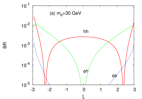
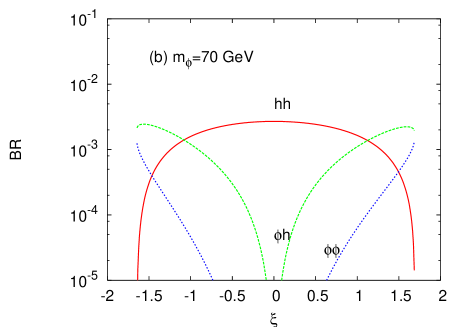
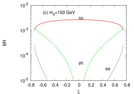
Figure 2: The branching ratios of the first KK graviton into two scalars as a function of $\xi$ for (a) $m_{\phi}=30$ GeV, (b) 70 GeV, and (c) 150 GeV. We set $m_{h}=120$ GeV, $\Lambda_{\phi}=5$ TeV and $m_{0}/M_{\rm Pl}=0.1$.

In Fig. 2, we show the small BR’s for $h_{\mu\nu}^{(1)}\to hh,h\phi,\phi\phi$ as a function of $\xi$ for $m_{\phi}=30,~{}70,~{}150$ GeV, respectively. As discussed before, we set $\Lambda_{\phi}=5$ TeV and $m_{0}/M_{\rm Pl}=0.1$. Note that if the radion-Higgs mixing is absent ($i.e.$, $\xi=0$), $h_{\mu\nu}^{(1)}\to h\phi,\phi\phi$ modes disappear. If $\xi\sim{\mathcal{O}}(1)$, the BR($h_{\mu\nu}^{(n)}\to h\phi$) for a light radion becomes compatible with BR($h_{\mu\nu}^{(n)}\to hh$), which is of order ${\mathcal{O}}(10^{-3})$.

IV Hadronic Production of Radion-Higgs pair

The leading-order sub-processes involved in the hadronic collisions for $pp(\bar{p})\to h\phi$ are

$$q\bar{q}\;\to\;h_{\mu\nu}^{(n)}\;\to\;h\phi\,,\quad gg\;\to\;h_{\mu\nu}^{(n)}\;\to\;h\phi\;.$$ (25)

It is clear from Eq. (16) that the gluon fusion process through KK graviton resonances is dominant for the associated production of the radion with the Higgs boson at hadronic colliders, especially at the LHC. Other subprocesses such as $q\bar{q}\to h^{*}(\phi^{*})\to h\phi$ are suppressed by the small Yukawa couplings. The other processes of $gg\to h^{*}(\phi^{*})\to h\phi$ are also suppressed since they occur at loop level and through virtual intermediate scalars. This is contrary to the subprocesses in Eq. (25) through the graviton poles where the majority of the cross section comes from.

The partonic cross sections for these two channels are given by

$$\frac{d\hat{\sigma}}{d\cos\theta^{*}}(gg\to h_{\mu\nu}^{(n)}\to h\phi) = \frac{\hat{g}^{2}_{Gh\phi}}{512\,\pi}\frac{\lambda^{5/2}}{\hat{s}}\left(\frac{\hat{s}}{\hat{\Lambda}_{W}^{2}}\right)^{2}\,|{\mathcal{D}}_{G}|^{2}\sin^{4}\theta^{*}~{},$$

$$\frac{d\hat{\sigma}}{d\cos\theta^{*}}(q\bar{q}\to h_{\mu\nu}^{(n)}\to h\phi) = \frac{\hat{g}^{2}_{Gh\phi}}{768\,\pi}\frac{\lambda^{5/2}}{\hat{s}}\left(\frac{\hat{s}}{\hat{\Lambda}_{W}^{2}}\right)^{2}\,\left|{\mathcal{D}}_{G}\right|^{2}\,\sin^{2}\theta^{*}\cos^{2}\theta^{*}~{},$$

where $\theta^{*}$ is the scattering angle in the incoming parton c.m. frame, $\lambda=(1-m^{2}_{h}/\hat{s}-m^{2}_{\phi}/\hat{s})^{2}-4(m_{h}^{2}/\hat{s})(m^{2}_{\phi}/\hat{s})$ and ${\mathcal{D}}_{G}$ is the KK graviton propagation factor, defined by Eq. (37). In the above equations, we use the Breit-Wigner prescription for the graviton propagator. When the c.m. energy is away from the graviton pole, the effect of the graviton width is negligible.

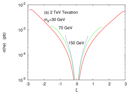
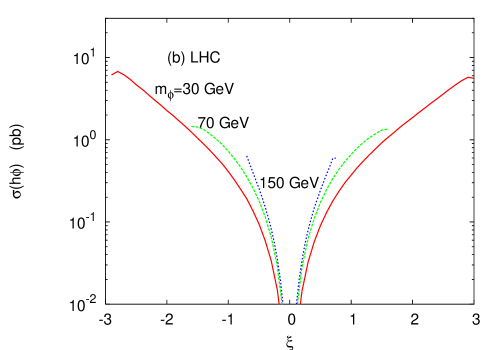
Figure 3: For $m_{\phi}=30,~{}70,~{}150$ GeV, total cross section for the associated production of the radion with the Higgs boson at (a) the 2 TeV Tevatron ($p\bar{p}$ collision) and (b) at the LHC ($pp$ collision at $\sqrt{s}=14$ TeV). As mentioned earlier, we always set $m_{h}=120$ GeV.

In Fig. 3, we plot the total cross section at the Tevatron ($\sqrt{s}=2$ TeV) and at the LHC ($\sqrt{s}=14$ TeV). In general, the cross section at the Tevatron is of order of fb, which means that we need a high luminosity option of the Tevatron in order to see the radion-Higgs mixing precisely. Fortunately, the background at the Tevatron can be reduced substantially without hurting the signal much (we shall show it in the next section). At a first glance, the situation at the LHC would be better: As can be seen in Fig. 3(b) the signal cross section increases by three orders of magnitude. For the lighter radion ($e.g.$, $m_{\phi}=30$ GeV) case, the cross section can reach above the pb level. Even for heavier radions with $m_{\phi}=150$ GeV, this rare process can produce a cross section close to the pb level if $\xi$ is sizable. However, one has to bear in mind that the QCD background increases more rapidly, as well as one has to take into account other backgrounds that were small at the Tevatron but large at the LHC. Therefore, we anticipate that Tevatron is in fact a better place than the LHC to search for the radion-Higgs mixing via the $h\phi\to b\bar{b}jj$ final state. In the next section, we show a detailed signal-background analysis of searching for the $h\phi$ mixing at the Tevatron using the $h\phi\to b\bar{b}jj$ decay mode.

For instructional purpose, we show the transverse momentum and invariant mass distributions in Fig. 4. The resonance structure due to KK graviton states is clear in both $p_{T}$ and invariant mass distributions.

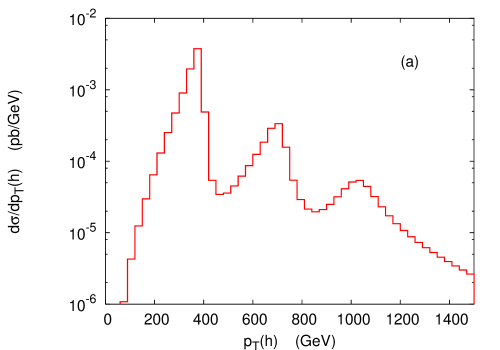
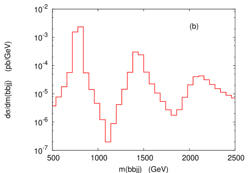
Figure 4: (a) Transverse momentum spectrum of the Higgs boson reconstructed from $h\to b\bar{b}$, and (b) the invariant mass $m(b\bar{b}jj)$ spectrum of the $h\phi$ system. We set $\Lambda_{\phi}=5~{}{\rm TeV}$, ${m_{0}}/{M_{\rm pl}}=0.1$, $\xi=1$ $m_{h}=120~{}{\rm GeV}$, and $m_{\phi}=30~{}{\rm GeV}$. We have applied a smearing $\Delta E/E=0.5/\sqrt{E}$, where $E$ in GeV, to all the final state particles, and we have imposed cuts $p_{T}(b,j)>20$ GeV.

V Decays and Detection of the Radion-Higgs pair

In this section, we consider the feasibility of detecting $h\phi$ pair production in the Run II at the Tevatron. For a Higgs boson of mass around $120$ GeV, the major decay mode is into $b\bar{b}$. The partial decay rate into $WW$ will begin to grow at $m_{H}\gtrsim 140$ GeV. Therefore, we shall focus on the $b\bar{b}$ mode for the Higgs boson decay. For a light radion with $m_{\phi}\mathrel{\raise 1.29167pt\hbox{$<$\kern-7.5pt\lower 4.30554pt\hbox{$\sim$}}}2m_{W}$, because of the QCD trace anomaly, the major decay mode of the radion is $gg$, followed by $b\bar{b}$ (a distant second). When the radion mass gets above the $WW$ threshold, the $WW$ mode becomes dominant. At the Tevatron, we only consider the light radion because the production cross section of the heavy radion is very small. Considering the following model parameters

$$\Lambda_{\phi}=5~{}{\rm TeV},\quad\frac{m_{0}}{M_{\rm pl}}=0.1,\quad m_{h}=120~{}{\rm GeV},\quad m_{\phi}=70~{}{\rm GeV},\quad\xi=1.5\,,$$ (26)

the production of the $h\phi$ pair will dominantly decay into $b\bar{b}gg$. The search for this final state is similar to the search for the associated production of $WH$ and $ZH$ with the hadronic decay of $W$ and $Z$ performed at CDF cdf-wh . We can follow their strategies to reduce the background.

The major background comes from the QCD heavy-flavor production of $b\bar{b}/c\bar{c}$ plus jets. Here the $c\bar{c}$ pair can also fake the $b$-tagging with a lower probability than the $b$ quark. We calculate the QCD $b\bar{b}+2$ jet background by a parton-level calculation, in which the sub-processes are generated by MADGRAPH madgraph . Typical cuts on detecting the $b$-jets and light jets are applied:

$$p_{T}(b)>15\;{\rm GeV}, \;p_{T}(j)>15\;{\rm GeV},$$

$$|y(b)|<2.5, \;|y(j)|<2.5,\;$$

$$\Delta R(k,l)>0.4\;\; \mbox{where $k,l=b,j$}\;.$$

We have applied a Gaussian smearing $\Delta E/E=0.5/\sqrt{E/{\rm GeV}}$ to the final-state $b$-jets and light jets, in order to simulate the detector resolution. Since the Higgs boson is produced together with a radion mainly via an intermediate graviton KK state, the Higgs boson tends to have a large $p_{T}\sim m_{G^{(1)}}/2$. Therefore, a transverse momentum cut on the $b\bar{b}$ pair is very efficient against the QCD background while only hurts the signal marginally. Figure 5 shows the $p_{T}(b\bar{b})$ distribution. We shall apply a cut

$$p_{T}(b\bar{b})>250\;{\rm GeV}$$ (27)

to reduce the background. The $b\bar{b}+2$ jet background is reduced to the $0.1\%$ level. There are other backgrounds such as $t\bar{t}$ production, $Z+$jets with $Z\to b\bar{b},c\bar{c}$, $Wb\bar{b},Wc\bar{c},Zb\bar{b},Zc\bar{c}$, and diboson and single top production, which only make up to about 1% of the total background.

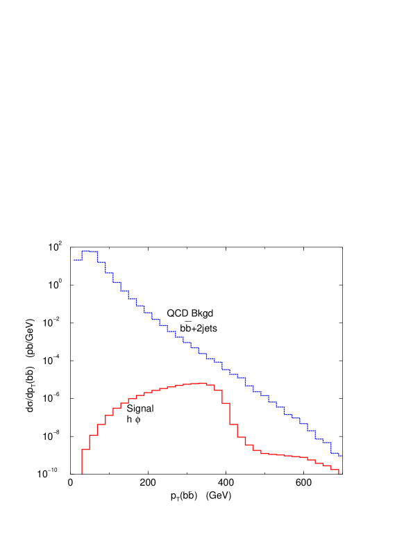
Figure 5: The transverse momentum distribution of the $b\bar{b}$ pair of the signal and the QCD background at Tevatron with $\sqrt{s}=2$ TeV. We set $\Lambda_{\phi}=5~{}{\rm TeV}$, ${m_{0}}/{M_{\rm pl}}=0.1$, $m_{h}=120~{}{\rm GeV}$, and $m_{\phi}=70~{}{\rm GeV}$, and $\xi=1.5$. The imposed cuts are $p_{T}(b,j)>15$ GeV, $|y(b,j)|<2.5$, and $\Delta R(k,l)>0.4$, where $k,l=b,j$.

The background is still $2-3$ orders of magnitude larger than the signal. We further impose the mass cut on the $b\bar{b}$ and $jj$ pair by requiring their invariant masses being close to the Higgs and radion masses, respectively:

$$|m(b\bar{b})-m_{H}|<10\;{\rm GeV},\;\;|m(jj)-m_{\phi}|<10\;{\rm GeV}\;.$$ (28)

The background is reduced to the same level as the signal: The signal cross section is about $0.66$ fb while the background cross section is about $0.94$ fb (which may vary $\sim 50\%$ due to changes in the renormalization scale). Further stringent cuts may help improve the signal-to-background ratio, but it would suppress the signal event rate to an unobservable level even at a $20$ fb^-1 luminosity.

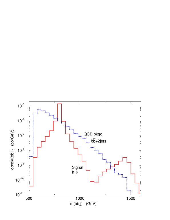
Figure 6: The invariant mass distribution of the $b\bar{b}jj$ of the signal and the QCD background after applying all the cuts described in the previous figure caption, Eq. (27), and Eq. (28).

The mass cuts of Eq. (28) can be imposed because the Higgs boson and the radion should have been observed before we search for their mixing effects. We can now look at the invariant mass distribution of the Higgs boson and the radion. We show it in Fig. 6. It is easy to see the peaks due to the graviton KK states.

So far we do not consider the signal-background analysis at the LHC. The obvious reason is that the situation at the LHC is actually getting worse. Although the signal is increasing by three orders of magnitude, the background grows much faster. Not only the $b\bar{b}jj$ background that we considered, we also have to consider other backgrounds such as $t\bar{t}$, $Wb\bar{b}$, and $Zb\bar{b}$, because they are no longer negligible at the LHC. Therefore, we anticipate that Tevatron is in fact a better place than the LHC to search for the mixing via the $h\phi\to b\bar{b}jj$ final state. If we could not find any evidence for radion-Higgs mixing in the mass range (low to intermediate Higgs and radion mass) that we are considering at the Tevatron, it would be even harder to do so at the LHC. Unless, if one looks into another mass range of the Higgs boson and radion, say, when the radion is heavier than $2m_{Z}$, then the golden mode $\phi\to ZZ\to 4l$ becomes very accessible. In this case, the LHC would be a good place to search for the mixing.

VI Conclusions

In the original Randall-Sundrum scenario where all the SM fields are confined on the visible brane, the radion-Higgs mixing is weakly suppressed by the radion VEV at the electroweak scale. We have studied the phenomenological signatures of this radion-Higgs mixing at hadron colliders. High energy processes exclusively allowed for non-zero mixing have been shown to provide complementary and valuable information for the mixing. In particular, the vertex of $h_{\mu\nu}^{(n)}$-$h$-$\phi$, one of four triple-vertices which would vanish without the radion-Higgs mixing, is expected to have the largest strength in the limit of the large radion VEV, $i.e.$, $v_{0}\ll\Lambda_{\phi}$, as suggested by the electroweak precision data.

We have studied all the partial decay widths of the KK gravitons in the presence of the radion-Higgs mixing. The decay mode into a gluon pair is dominant. If the radion-Higgs mixing parameter $\xi$ is of order one, the decay rate into a radion and a Higgs boson becomes as large as that into a Higgs boson pair, with the branching ratio of order $10^{-3}$.

At hadron colliders, it is feasible to produce the KK graviton resonances, followed by their decay into a radion and a Higgs boson, which is a clean signatures for the radion-Higgs mixing. We have performed a signal-background analysis at the 2 TeV Tevatron, restricting ourselves to the intermediate mass range for the Higgs boson and the radion (otherwise the cross section at the Tevatron would be too small to start with). The dominant decay mode is the $h\phi\to b\bar{b}gg$. Using the strategic cuts that we devised in this work, we have been able to reduce the major QCD background of $b\bar{b}+2j$ production to the same level as the signal. With an integrated luminosity of 20 fb^-1 that one can hope for the Run II, one may be able to see a handful of such events. We anticipate the situation at the LHC is not improving for this intermediate mass range of Higgs and radion, because the QCD background increases much faster than the signal. On the other hand, if one looks into the heavier mass range of the radion, say, when the radion is heavier than $2m_{Z}$, then the golden mode of $\phi\to ZZ\to 4l$ becomes very accessible. In this case, the final state would consist of $h\phi\to b\bar{b}\ell^{+}\ell^{-}\ell^{+}\ell^{-}$, which is very striking. Then the LHC would be a good place to search for the mixing.

Appendix A Feynman Rules

Figure 7: Feynman rules for the tri-linear vertices in the scalar sector. In the $h_{\mu\nu}^{n}$ vertices, we have made use of the symmetry of $h_{\mu\nu}^{n}$ under $\mu\leftrightarrow\nu$.

Feynman rules relevant for the Higgs-radion production at hadron colliders are to be summarized, focused on trilinear vertices as depicted in Fig. 7. Properly normalized vertex factors are

$$\hat{g}_{Gh\phi} = 6\gamma\xi\left[a(\gamma b+d)+bc\right]+cd\,,$$ (29)

$$\hat{g}_{G\phi\phi} = 6a\gamma\xi\left[a\gamma+2c\right]+c^{2}\,,$$

$$\hat{g}_{Ghh} = 6b\gamma\xi\left[b\gamma+2d\right]+d^{2}\,.$$

In the limit of $\xi\to 0$, we have

$$\lim_{\xi\to 0}\hat{g}_{{}_{Ghh}}=1,\quad\lim_{\xi\to 0}\hat{g}_{{}_{G\phi h}}=0,\quad\lim_{\xi\to 0}\hat{g}_{{}_{G\phi\phi}}=0.$$ (30)

The $h-h-\phi$ and $\phi-h-\phi$ vertices involve $q^{2}$-dependent couplings $\hat{g}_{h,\phi}$, parameterized by

$$\hat{g}_{\phi} = \hat{g}_{\phi 1}(1+\mu_{\phi}^{2})+\hat{g}_{\phi 2}\,\mu_{h}^{2}-\hat{g}_{\phi 3}\,\mu_{h_{0}}^{2}\,,$$ (31)

$$\hat{g}_{h} = \hat{g}_{h1}(1+\mu_{h}^{2})+\hat{g}_{h2}\,\mu_{\phi}^{2}-\hat{g}_{h3}\,\mu_{h_{0}}^{2}\,,$$

where $\mu_{h,\phi}\equiv m_{h,\phi}/\sqrt{q^{2}}$ ($\mu_{h_{0},\phi_{0}}\equiv m_{h_{0},\phi_{0}}/\sqrt{q^{2}}$), and

$$\hat{g}_{h1} = 6b\xi\Bigl{\{}\gamma(ad+bc)+cd\Bigr{\}}+ad^{2}\,,\quad\quad\;\hat{g}_{\phi 1}=6a\xi\Bigl{\{}\gamma(ad+bc)+cd\Bigr{\}}+bc^{2}\,,$$ (32)

$$\hat{g}_{h2} = d\left\{12ab\gamma\xi+2bc+ad(6\xi-1)\right\}\,,\quad\hat{g}_{\phi 2}=c\left\{12ab\gamma\xi+2ad+bc(6\xi-1)\right\}\,,$$

$$\hat{g}_{h3} = 4d(ad+2bc)+3\gamma^{-1}cd^{2}\,,\quad\quad\quad\quad~{}\hat{g}_{\phi 3}=4c(2ad+bc)+3\gamma^{-1}c^{2}d\,.$$

Figure 8: Feynman rules involving gluon pair.

For completion, we review the Feynman rules involving a gluon pair in Fig. 8. We refer for the expressions of $C_{\mu\nu,\rho\sigma}$ and $D_{\mu\nu,\rho\sigma}$ to Ref. Han-Zhang , and

$$\hat{c}_{h} = -\frac{\alpha_{s}}{4\pi}\left[(d+\gamma b)\sum_{i}F_{1/2}(4\mu^{2}_{ih})-2b_{3}\gamma b\right]\,,$$ (33)

$$\hat{c}_{\phi} = -\frac{\alpha_{s}}{4\pi}\left[(c+\gamma a)\sum_{i}F_{1/2}(4\mu^{2}_{i\phi})-2b_{3}\gamma a\right]\,.$$

Here $F_{1/2}(x)=-2x[1+(1-x)f(x)]$ and $f(x)=-(1/4)\ln\left[(\sqrt{1-x}+1)/(\sqrt{1-x}-1)\right]^{2}$ with $\mu_{ij}\equiv m_{i}/m_{j}$.

Appendix B Helicity amplitudes for $gg\to h\phi$ and $q\bar{q}\to h\phi$

For the gluon fusion process of

$$g(q_{1},\lambda_{1})+g(q_{2},{\lambda}_{2})\rightarrow h(k_{1})+\phi(k_{2})\,,$$ (34)

four momenta in the parton c.m. frame are defined by

$$q_{1}^{\mu}\!\! = \!\!\frac{\sqrt{\hat{s}}}{2}\left(1,0,0,1\right),\quad q_{2}^{\mu}=\frac{\sqrt{\hat{s}}}{2}\left(1,0,0,-1\right),$$ (35)

$$k_{1}^{\mu}\!\! = \!\!\frac{\sqrt{\hat{s}}}{2}\left(1+\mu_{h}^{2}-\mu_{\phi}^{2},\phantom{-}\lambda^{\frac{1}{2}}\sin\theta^{*},0,\phantom{-}\lambda^{\frac{1}{2}}\cos\theta^{*}\right),$$

$$k_{2}^{\mu}\!\! = \!\!\frac{\sqrt{\hat{s}}}{2}\left(1-\mu_{h}^{2}+\mu_{\phi}^{2},-\lambda^{\frac{1}{2}}\sin\theta^{*},0,-\lambda^{\frac{1}{2}}\cos\theta^{*}\right),$$

where $\mu_{h,\phi}\equiv m_{h,\phi}/\sqrt{\hat{s}}$, $|\vec{p}_{h}|=|\vec{p}_{\phi}|=\lambda^{\frac{1}{2}}\sqrt{\hat{s}}/2$ and $\lambda=1+\mu_{h}^{4}+\mu_{\phi}^{4}-2\mu_{h}^{2}-2\mu_{h}^{2}-2\mu_{h}^{2}\mu_{h}^{2}$. The $\lambda_{1(2)}=\pm$ denotes the gluon polarization, which specifies its polarization vectors as

$$\epsilon^{\mu}_{1}(q_{1},\lambda_{1})=\frac{1}{\sqrt{2}}\left(0,-\lambda_{1},-i,0\right),\quad\epsilon^{\mu}_{2}(q_{2},\lambda_{2})=\frac{1}{\sqrt{2}}\left(0,\lambda_{2},-i,0\right).$$ (36)

Defining the propagator factors of the KK-graviton, Higgs and radion by

$${\mathcal{D}}_{G}=\sum_{n=1}^{\infty}\frac{\hat{s}}{\hat{s}-m^{2}_{G^{(n)}}+im_{G^{(n)}}\Gamma_{G^{(n)}}}\,,\quad{\mathcal{D}}_{h,\phi}=\frac{\hat{s}}{\hat{s}-m_{h,\phi}^{2}+im_{h,\phi}\Gamma_{h,\phi}}\,,$$ (37)

the helicity amplitudes $\delta^{ab}{\mathcal{M}}_{\lambda_{1},\lambda_{2}}$ with the color factor of $\delta^{ab}$ are

$${\mathcal{M}}_{++} = -\frac{\hat{s}}{2v\Lambda_{\phi}}\left(\hat{c}_{h}\hat{g}_{h}\mathcal{D}_{h}+\hat{c}_{\phi}\hat{g}_{\phi}\mathcal{D}_{\phi}\right),$$ (38)

$${\mathcal{M}}_{+-} = -\frac{\hat{s}\lambda}{\widehat{\Lambda}_{W}^{2}}\hat{g}_{G\phi h}\mathcal{D}_{G}\sin^{2}\theta^{*}\,,$$

where ${\mathcal{M}}_{++}={\mathcal{M}}_{--}$ and ${\mathcal{M}}_{+-}={\mathcal{M}}_{-+}$ guarantied by CP invariance. Note that the contribution of the scalar mediation is separated from that of KK gravitons according to the gluon polarization.

For the differential cross section of

$$\frac{d\hat{\sigma}}{d\cos\theta^{*}}=\frac{\lambda^{1/2}}{32\pi\hat{s}}\overline{|{\mathcal{M}}|^{2}}\,,$$ (39)

the gluon-polarization averaged amplitude squared is

$$\overline{|{\mathcal{M}}|^{2}}=\frac{1}{2}\cdot\frac{1}{2}\cdot\frac{1}{8}\cdot\frac{1}{8}\cdot 8\left[|{\mathcal{M}}_{++}|^{2}+|{\mathcal{M}}_{+-}|^{2}+|{\mathcal{M}}_{-+}|^{2}+|{\mathcal{M}}_{--}|^{2}\right]\,,$$ (40)

where the factor $1/2$ is for the gluon polarization average, the factor $1/8$ for the gluon color average, and the factor $8$ for the color-sum.

For the $q\bar{q}$ annihilation production of the Higgs and radion, the helicity amplitudes are the same as the case of $e^{+}e^{-}\to h\phi$ except for the color factor ours . Coordinating notations, we have

$$\overline{|{\mathcal{M}}|^{2}}(q\bar{q}\to h\phi)=\frac{\hat{g}_{G\phi h}^{2}}{24}\left(\frac{\lambda\hat{s}}{\widehat{\Lambda}_{W}^{2}}\right)^{2}|\mathcal{D}_{G}|^{2}\sin^{2}\theta^{*}\cos^{2}\theta^{*}\,.$$ (41)

References

(1)
See, , J. F. Gunion, H. E. Haber, G. L. Kane and S. Dawson, The Higgs Hunter’s Guide (Addison-Wesley, Reading, MA, 1990).
(2)
R. Chivukula, B. Dobrescu, and E. Simmons, Phys. Lett. B401, 74 (1997).
(3)
M. J. Duncan, G. L. Kane and W. W. Repko,
Nucl. Phys. B272, 517 (1986).
(4)
G. Abbiendi et al., The LEP Working Group for Higgs Boson Searches,
Phys. Lett. B565, 61 (2003).
(5)
LEP Electroweak Working Group, Report no. LEPEWWG/2002-01.
(6)
L. Randall, R. Sundrum,
Phys. Rev. Lett. 83, 3370 (1999);
L. Randall, R. Sundrum,
Phys. Rev. Lett. 83, 4690 (1999).
(7)
W. D. Goldberger and M. B. Wise,
Phys. Rev. Lett. 83, 4922 (1999);
W. D. Goldberger and M. B. Wise,
Phys. Lett. B475, 275 (2000).
(8)
C. Csaki, M. Graesser, L. Randall and J. Terning,
Phys. Rev. D62, 045015 (2000).
(9)
S. B. Bae, P. Ko, H. S. Lee and J. Lee,
Phys. Lett. B487, 299 (2000).
(10)
G. F. Giudice, R. Rattazzi and J. D. Wells,
Nucl. Phys. B595, 250 (2001).
(11)
C. Csaki, M. L. Graesser and G. D. Kribs,
Phys. Rev. D63, 065002 (2001);
C. S. Kim, J. D. Kim and Jeonghyeon Song,
Phys. Lett. B511, 251 (2001);
C. S. Kim, J. D. Kim and Jeong-hyeon Song,
Phys. Rev. D67, 015001 (2003).
(12)
U. Mahanta and S. Rakshit,
Phys. Lett. B480, 176 (2000);
K. Cheung,
Phys. Rev. D63, 056007 (2001);
U. Mahanta and A. Datta,
Phys. Lett. B483, 196 (2000);
S. C. Park, H. S. Song and J. Song,
Phys. Rev. D65, 075008 (2002);
S. C. Park, H. S. Song and J. Song,
Phys. Rev. D63, 077701 (2001);
C. S. Kim, Kang Young Lee and Jeonghyeon Song,
Phys. Rev. D64, 015009 (2001).
(13)
M. Chaichian, A. Datta, K. Huitu and Z. Yu,
Phys. Lett. B524, 161 (2002).
(14)
T. Han, G. D. Kribs and B. McElrath,
Phys. Rev. D64, 076003 (2001).
(15)
J. L. Hewett and T. G. Rizzo,
arXiv:hep-ph/0202155.
(16)
D. Dominici, B. Grzadkowski, J. F. Gunion and M. Toharia,
arXiv:hep-ph/0206192.
(17)
K. Cheung, C.S. Kim, and J.-H. Song, Phys. Rev. D67, 075017 (2003).
(18)
H. Davoudiasl, J. L. Hewett and T. G. Rizzo,
Phys. Rev. D63, 075004 (2001).
(19)
H. Davoudiasl, J. L. Hewett and T. G. Rizzo,
Phys. Lett. B473, 43 (2000).
(20)
Talk by E.J. Thompson at SLAC Summer Institute, August 2003,
available at http://www-cdf.fnal.gov/physics/talks_transp/2003/slac_tevresults_thomson.pdf.
(21)
F. Abe et al. (CDF Coll.), Phys. Rev. Lett. 81, 5748 (1998).
(22)
T. Stelzer and W.F. Long, Comput. Phys. Commun. 81, 357 (1994);
F. Maltoni and T. Stelzer, JHEP 0302, 027 (2003).
(23)
T. Han, J. D. Lykken and R. J. Zhang,
Phys. Rev. D 59, 105006 (1999).