TAUP 2006-92

November, 1992

Pair production in a strong electric field:
an initial value problem in quantum field
theory

Y. Kluger, J. M. Eisenberg, and B. Svetitsky
 
School of Physics and Astronomy
Raymond and Beverly Sackler Faculty
of Exact Sciences
Tel Aviv University
69978 Tel Aviv, Israel

ABSTRACT. We review recent achievements in the solution of the initial-value problem for quantum back-reaction in scalar and spinor QED. The problem is formulated and solved in the semiclassical mean-field approximation for a homogeneous, time-dependent electric field. Our primary motivation in examining back-reaction has to do with applications to theoretical models of production of the quark-gluon plasma, though we here address practicable solutions for back-reaction in general. We review the application of the method of adiabatic regularization to the Klein-Gordon and Dirac fields in order to renormalize the expectation value of the current and derive a finite coupled set of ordinary differential equations for the time evolution of the system. Three time scales are involved in the problem and therefore caution is needed to achieve numerical stability for this system. Several physical features, like plasma oscillations and plateaus in the current, appear in the solution. From the plateau of the electric current one can estimate the number of pairs before the onset of plasma oscillations, while the plasma oscillations themselves yield the number of particles from the plasma frequency.

We compare the field-theory solution to a simple model based on a relativistic Boltzmann-Vlasov equation, with a particle production source term inferred from the Schwinger particle creation rate and a Pauli-blocking (or Bose-enhancement) factor. This model reproduces very well the time behavior of the electric field and the creation rate of charged pairs of the semiclassical calculation. It therefore provides a simple intuitive understanding of the nature of the solution since nearly all the physical features can be expressed in terms of the classical distribution function.

1 Introduction

This review deals with the physical situation in which initially there exists a classical electric field out of which pairs of charged particles tunnel. The particles are accelerated by the field, producing a current and, in the sequel, a field that acts counter to the original one. Eventually, plasma oscillations are set up. This so-called back-reaction problem has been of considerable interest in recent years in particle physics, serving for example as a model of the production of the quark-gluon plasma. One supposes that when two nuclei collide at ultra-relativistic energies, they induce color charges on each other. Passing through each other, they leave in their wake a color electric field from which quarks and gluons emerge more or less according to the above scenario. Of course, the color electric field is non-Abelian, whereas we take it to be Abelian in the version of the back-reaction problem we defined above. Furthermore, the field does not fill all space homogeneously, a condition that thus far one has had to impose in order to carry out practical calculations, as we shall discuss below.

Back reaction has been studied intensively in recent years in the domain of inflationary cosmology, where instead of a time-varying electric field one has the time-dependent gravitational metric. Again pairs emerge via tunneling and then act back on the field, in this case through their masses.

Our own interest in the back-reaction problem was sparked by its application to the quark-gluon plasma problem, and it is therefore almost exclusively in these terms that we shall present our discussion here. Much of the evolution of regularization and renormalization methods for the back-reaction problem [1–17] has taken place, however, in the context of inflationary cosmology. In this area there exists a sizable literature, summarized—except, of course, for the more recent developments—in the books of Birrell and Davies [18] and of Fulling [19]. Earlier surveys of the status of this problem can be found in the reviews of Zel’dovich [20] and of DeWitt [21]. We shall not describe these developments here, but rather pick up our discussion with the treatment of adiabatic regularization given by Cooper and Mottola [16], which has proved an adequate starting point for the practicable calculational schemes upon which we focus.

In concentrating on methods that lead to workable calculations for back-reaction, we shall not address the vast number of papers that deal primarily or exclusively with the Schwinger mechanism [22–27] and its many applications such as the flux-tube model [29–32]; nor shall we touch on the generalizations of this mechanism to handle pair production in given, external, time-dependent electric fields, reviewed in Refs. [33, 34]; nor do we deal with the various efforts to consider pair production in restricted volumes [35]. We shall restrict ourselves to methods based on adiabatic regularization for the renormalization of the electric current or on methods that have been shown [5, 9, 18, 19] to be equivalent to it.

Interest in back-reaction in the context of the quark-gluon plasma (QGP) arose through work of Białas and Czyż and coworkers [39, 40], of Kajantie and Matsui [41], and of Gatoff, Kerman, and Matsui [42]. In these series of studies, the authors modeled the production and early dynamics of the QGP by considering a transport equation for quarks or gluons, on the right-hand side of which appears a source term based on the Schwinger formula for pair production in an electric field fixed in time. The electric field is, in turn, governed by Maxwell’s equations, with the current of the produced pairs figuring in the time evolution of the electric field. This coupled system is solved, and the subsequent development exhibits plasma oscillations and other distinctive behavior (as we shall see in our discussion here).

The genesis of the classical transport equation, while intuitively very appealing, is far from self-evident: The whole point in back-reaction is that the electric field must change in response to the current of produced pairs, so that the assumption of a fixed field, inherent in the Schwinger formula, is out of place. Furthermore, when one imagines deriving a transport equation directly from the field equations through the well-known procedure of the Wigner transformation [43], it is clear that the equation cannot lead directly to a source term. Since the Wigner treatment is completely general, it follows that in any quantum mechanical treatment there is no possible separation between the role of the electric field in accelerating charged particles and its role in producing these particles out of the vacuum through tunneling. Thus it is quite mysterious how a classical transport equation can arise in this formalism.

In order to examine back-reaction in detail, we return to the original initial-value problem in quantum field theory. We write a coupled set of field equations for charged particles in interaction with an electric field. For purposes of comparing with the models [39–42] for the QGP, it is adequate to take this electric field as classical. (Purists may note that this is the leading order in a $1/N$ expansion, where $N$ is the number of flavors of the matter field.) Clearly one will wish eventually to consider a quantized electromagnetic field (i.e., higher orders in $1/N$) so as to incorporate the essential physics of radiation for more realistic applications. The specification of initial conditions for the matter field reduces the field equations to $c$-number differential equations. This development was carried out initially for bosons [16, 50], and is presented here in Section 2.

The numerical solution of these coupled equations is confronted by two obstacles: (i) The field equations must be renormalized in order to render them finite, and (ii) it emerges that the calculated momentum distribution of the produced particles is highly oscillatory so that great care is required to produce reliable numerical results. The first of these problems is solved by taking as a starting point the extensive work noted earlier in renormalizing the pair-production problem for inflationary cosmology [1–19], though, as we shall see, some modifications to this procedure are required in practice. Unfortunately, the available techniques limit us to the case of a spatially homogeneous electric field. Overcoming the second obstacle merely requires sufficient computer power to achieve long-range numerical stability in spite of short-range oscillations. These points are developed in some detail in Section 2. We there review results [50] in $1+1$ dimensions and present results in $3+1$ dimensions for the first time.

Somewhat to our surprise, the classical transport equation used [39–42] for the QGP permits very nearly a quantitative simulation of the field-theory result, thus considerably bolstering one’s belief in the legitimacy of various detailed steps involved at the technical level in both procedures. The agreement between the two procedures is greatly improved by including in the transport equation a term that provides for Bose-Einstein enhancement in the production process; this term is found to have a particular form which is motivated by careful consideration of pair production in an external classical electric field.

The treatment of fermion pair production [51], presented in Section 3, involves some technical issues concerning the use of the adiabatic regularization procedure. The physics of Pauli blocking makes it rather less evident that a classical transport equation can succeed here, so it is, perhaps, even more surprising than for bosons that a classical transport equation gives an adequate description of the results, even at a quantitative level. In this case, good agreement requires the introduction of an explicit Pauli-blocking factor in the transport equation.

The application to the QGP requires going beyond the case of a uniform electric field. Luckily, one can take advantage of the approximate invariance under longitudinal boosts which is often assumed in modeling particle production in the central rapidity region [52, 53]. The transformation of the field equations to comoving coordinates allows renormalization just as in the case of the homogeneous electric field, and numerical solution follows [54]. We do not review these developments here.

The work covered here treats a highly-idealized situation of a classical electric field, homogeneous in space and producing particles that possess no mutual interactions. This can at best serve as a starting point for more serious studies that contain the complications that are essential for physical applications. However, we feel that the beginning phase is now more or less complete, and therefore is deserving of review here. The incorporation of particle scattering and of bremsstrahlung is straightforward, and such work is in progress. Lifting the restriction of spatial homogeneity (or of boost invariance), on the other hand, appears very difficult.

2 Boson pair production

2.1 Introduction

Beginning with Sauter’s pioneering paper [22] in 1931, the problem of spontaneous pair production in the presence of an external electric field has been investigated by many authors [23–27, 33, 34]. The most commonly used formula for the spontaneous pair creation rate per unit volume, derived by Schwinger [24], is based on a field-theory calculation for a constant and homogeneous electric field $E$, to all orders in $E,$

$$w=(2s+1)\frac{m^{4}}{(2\pi)^{3}}\left(\frac{E}{E_{0}}\right)^{2}\sum_{n=1}^{\infty}\frac{\beta_{n}}{n^{2}}\exp(-n{\pi}E_{0}/E)\ ,$$ (2.1)

where $s$ is the spin of the particles produced, ${\beta_{n}}=(-1)^{n-1}$ for bosons and ${\beta_{n}}=1$ for fermions, and $E_{0}=m^{2}/e$. This formula has been used extensively in modeling particle production in the central rapidity region in high-energy nucleus–nucleus collisions [39–42, 55, 56].

In this expression the electric field is held constant by an external agent. Thus, there is no effect of the produced particles on the original electric field—no back-reaction. Moreover, the mutual interactions of the particles are not taken into account. As long as the intensity of the initial electric field is small, $E{\ll}E_{0}$, Schwinger’s formula is valid. However, when it is applied for a strong electric field, $E>E_{0}$, it gives $w\propto(E/E_{0})^{2}$, violating unitarity for sufficiently strong fields [33]. In such circumstances it is necessary to include both the interaction between the particles created and the screening of the external field.

As discussed in Section 1, we assume that the electric field is classical, Abelian, and homogeneous. We impose the restriction to a spatially uniform electric field not just for simplicity, but also to dispose of infinities that would otherwise appear in the expectation value of the current operator in the Maxwell equation. These infinities are removed by adiabatic regularization and renormalization. It is important to note that in an initial value problem the divergences in the expectation values of the electric current or the energy-momentum tensor are time dependent. Nonetheless, the charge and mass renormalizations are time-independent and the infinities which appear in the currents are products of time-independent infinite quantities with time-dependent finite quantities.

A scheme for solving the quantum back-reaction problem in scalar QED was put forth by Cooper and Mottola [16]. Some analytical progress based on this scheme has been made [17], but is limited to very short times or very weak electric fields. In order to see substantial pair production and the subsequent onset of plasma oscillations we need to begin with a strong initial electric field, $E\sim E_{0}$, and to follow the evolution to large times, $t{\gg}m/eE$. It is useful to investigate the problem in 1+1 dimensions as a first step in testing numerical procedures since there are no transverse momenta to take into account, and since renormalization is relatively trivial. We then proceed to $3+1$ dimensions.

Adiabatic regularization will only render the theory finite if we impose a special initial configuration of the charged matter field—the adiabatic vacuum. This does not mean that there are no particles in the initial state. As long as the matter field and the electric field interact with each other, the expectation value of the number operator is not equal to the asymptotic particle number density, and even this adiabatic vacuum may contain a nonzero density. Nonadiabatic initial conditions would introduce infinities into the time derivatives of the current at $t=0$. Ultimately, the physical behavior we find in our calculations offers us a way to determine an effective particle density during the evolution of the system.

2.2 Pair production in semiclassical scalar QED

Equations of motion and second quantization

The scalar QED coupled equations of motion in the mean-field approximation (and without a $\phi^{4}$ self-interaction term as included in [16]) are given by the Klein-Gordon equation

$$[(\partial^{\mu}+ieA^{\mu})(\partial_{\mu}+ieA_{\mu})+m^{2}]\Phi(x)=0$$ (2.2)

and the semiclassical Maxwell equations

$$\partial_{\mu}F^{\mu\nu}=\langle i|j^{\nu}|i\rangle,$$ (2.3)

where $|i\rangle$ is the initial configuration of the charged matter field, and the current $j^{\nu}$ of the charged scalar field is symmetrized in order to be odd under charge conjugation,

$$j^{\nu}=\frac{ie}{2}[\Phi^{\dagger}(D^{\nu}\Phi)-(D^{\nu}\Phi)^{\dagger}\Phi-\Phi(D^{\nu}\Phi)^{\dagger}+(D^{\nu}\Phi)\Phi^{\dagger}].$$

Here $D^{\nu}=\partial^{\nu}+ieA^{\nu}$ is the covariant derivative. Note that the expectation value $\langle i|j^{\nu}|i\rangle$ does not vanish because $|i\rangle$ cannot be an eigenstate of the charge-conjugation operator as long as a time-varying electric field is present. As we shall see this expectation value is divergent, and available practical schemes which remove this divergence are, at the moment, limited to the case of spatially homogeneous electric fields [18, 19]. This homogeneity reduces the Maxwell equations to a single equation

$$\frac{\partial^{2}{\bf A}}{\partial t^{2}}=\langle i|{\bf j}|i\rangle.$$ (2.4)

The scalar charge density $j^{0}$ vanishes everywhere because of Gauss’ Law, and the magnetic field is a constant which we choose to be zero. We have selected the gauge $A_{0}=0$, and we choose E to lie along the $z$ axis. Thus $A_{z}$ is the only nonvanishing component, $A^{\nu}=(0,0,0,A(t))$.

Spatial homogeneity enables us to express the boson field operator $\Phi$ as a Fourier integral in which the coefficients are the Heisenberg operators $a_{\bf k}(t)$ and ${b_{-{\bf k}}}^{\dagger}(t)$,

$$\Phi(x,t)=\int\frac{[d{\bf{k}}]}{\sqrt{2{\omega_{\bf k}}^{0}}}\,e^{i{\bf k}\cdot\bf x}\,[a_{\bf k}(t)+{b_{-{\bf k}}}^{\dagger}(t)]\ ,$$ (2.5)

where $\omega_{\bf k}^{0}=\sqrt{{\bf k}^{2}+m^{2}}$ and $[d{\bf k}]={d^{d}{\bf k}}/{(2\pi)^{d}},$ with $d$ the spatial dimension. Using the Klein-Gordon equation (2.2), the operator $O_{\bf k}(t)=a_{\bf k}(t)+{b_{-{\bf k}}}^{\dagger}(t)$ satisfies

$$\frac{d^{2}O_{\bf k}}{dt^{2}}+\omega_{\bf k}^{2}(t)O_{\bf k}=0\ ,$$ (2.6)

where

$$\omega_{{\bf k}}(t)^{2}=[{\bf k}-e{\bf{A}}(t)]^{2}+m^{2}\ .$$ (2.7)

Since $\omega_{\bf k}(t)$ is a $c$-number, the annihilation and creation operators $a_{\bf k}(t)$ and ${b_{-{\bf k}}}^{\dagger}(t)$ can be expressed in terms of $a_{\bf k}(0)$ and ${b_{-{\bf k}}}^{\dagger}(0)$ by means of a Bogolyubov transformation,

$$a_{\bf k}(t) = u_{\bf k}(t)a_{\bf k}(0)+v_{\bf k}(t){b_{-{\bf k}}}^{\dagger}(0)$$

$${b_{-{\bf k}}}^{\dagger}(t) = {v_{\bf k}}^{\ast}(t)a_{\bf k}(0)+{u_{\bf k}}^{\ast}(t){b_{-{\bf k}}}^{\dagger}(0).$$ (2.8)

It is convenient to rewrite $\Phi$ in terms of mode amplitudes,

$$f_{\bf k}(t)=\frac{u_{\bf k}(t)+{v_{\bf k}}^{\ast}(t)}{\sqrt{2{\omega_{\bf k}}^{0}}}\ ,$$

namely,

$$\Phi(x,t)=\int[d{\bf k}]\,[f_{\bf k}(t)a_{\bf k}(0)+f_{\bf k}^{\ast}(t)b_{-{\bf k}}^{\dagger}(0)]\,e^{i\bf{k}\cdot\bf{x}}\ .$$ (2.9)

Thus $f_{\bf k}$ satisfies Eq. (2.6),

$$\frac{d^{2}f_{\bf k}(t)}{dt^{2}}+\omega_{\bf k}^{2}(t)f_{\bf k}(t)=0\ .$$ (2.10)

The Bogolyubov coefficients are related to the $f_{\bf k}(t)$ by

$$u_{\bf k}(t)=\frac{i\dot{f_{\bf k}}+{\omega_{\bf k}}^{0}f_{\bf k}}{\sqrt{2{\omega_{\bf k}}^{0}}}\quad{\rm and}\quad v_{\bf k}(t)=\frac{i\dot{f_{k}}^{\ast}+\omega_{k}^{0}f_{k}^{\ast}}{\sqrt{2\omega_{k}^{0}}}\ .$$ (2.11)

The canonical commutation relations

$$[\Phi(t,{\bf x}),\Pi(t,{\bf{y}})]=i\delta^{(d)}(\bf{x}-\bf{y})$$ (2.12)

imply via (2.5) that

$$[a_{\bf k}(t),a_{\bf{q}}^{\dagger}(t)]=[b_{\bf k}(t),b_{\bf{q}}^{\dagger}(t)]={(2\pi)}^{d}\delta^{(d)}(\bf{k}-\bf{q})\ .$$

These relations will be satisfied if

$${|u_{\bf k}(t)|}^{2}-{|v_{\bf k}(t)|}^{2}=1\ ,$$ (2.13)

or, by (2.11),

$$f_{\bf k}\dot{f}_{\bf k}^{\ast}-f_{\bf k}^{\ast}\dot{f}_{\bf k}=i.$$ (2.14)

Since the Wronskian of Eq. (2.10) is time independent, this condition is satisfied automatically, provided that it is satisfied by the initial conditions $f_{\bf k}(0),\dot{f}_{\bf k}(0)$.

Eq. (2.14) implies that $f_{\bf k}(t)$ can be expressed in terms of the real and positive function $\Omega_{\bf k}(t)$,

$$f_{\bf k}(t)=\frac{1}{\sqrt{2\Omega_{\bf k}(t)}}\,\exp\left[-i\int^{t}\Omega_{\bf k}(t^{\prime})dt^{\prime}\right]\ ,$$ (2.15)

if $\Omega_{\bf k}(t)$ satisfies

$$\Omega^{2}_{\bf k}(t)=-\frac{\ddot{\Omega}_{\bf k}}{2\Omega_{\bf k}}+\frac{3}{4}{\left(\frac{\dot{\Omega}_{\bf k}}{{\Omega_{\bf k}}}\right)}^{2}+\omega^{2}_{\bf k}(t)\ .$$ (2.16)

The representation (2.15) of $f_{\bf k}$ in a WKB-like form enables us to obtain the WKB-like equation (2.16) for $\Omega_{\bf k}$, and will help us identify divergences in the expectation values of the current and the energy-momentum tensor.

The adiabatic expansion and the adiabatic vacuum

The effect of pair production is related [33] to the appearance of negative frequencies in the solution for $f_{\bf k}(t).$ Looked at naively, however, the parametrization (2.15) might seem to have only positive frequencies when the interaction with the electromagnetic field is switched off. In fact, this is not the case since $\Omega_{\bf k}(t)$ for large $t$ does not approach a constant. To see this, we express $f_{\bf k}(t)$ in a different manner using the addition formula [57]

$$f_{\bf k}(t) = \frac{1}{\sqrt{2\Omega_{\bf k}(t)}}\,\exp\left[-i\int^{t}\Omega_{\bf k}(t^{\prime})dt^{\prime}\right]$$ (2.17)

$$= \frac{1}{\sqrt{2W_{\bf k}(t)}}\left\{c_{1{\bf k}}\,\exp\left[-i\int^{t}W_{\bf k}(t^{\prime})dt^{\prime}\right]\right.$$

$$\left.\qquad\qquad\mbox{}+c_{2{\bf k}}\,\exp\left[+i\int^{t}W_{\bf k}(t^{\prime})dt^{\prime}\right]\right\}\ ,$$

where the constants $c_{1{\bf k}}$ and $c_{2{\bf k}}$ fulfill

$${|c_{1{\bf k}}|}^{2}-{|c_{2{\bf k}}|}^{2}=1$$ (2.18)

and where $W_{\bf k}(t)$ satisfies the same equation of motion (2.16) as does $\Omega_{\bf k}(t)$. According to a theorem in asymptotic expansions, which is related to the generalized WKB or Liouville-Green approximation, if $\omega\in C^{\infty}$, the solutions of (2.10) are linear combinations of basis solutions [the right-hand side of (2.17)] which can be approximated as [19, p. 154]

$$f_{\bf k}^{\pm}(t) \equiv \frac{1}{\sqrt{2W_{\bf k}(t)}}\,\exp\left[\mp i\int^{t}W_{\bf k}(t^{\prime})dt^{\prime}\right]$$

$$= \frac{1}{\sqrt{2W^{\rm ad}_{\bf k}(t)}}\,\exp\left[\mp i\int^{t}W^{\rm ad}_{\bf k}(t^{\prime})dt^{\prime}\right]+O(\omega^{-N}_{\bf k})$$

$$W^{\rm ad}_{\bf k}(t)^{2} = \omega_{\bf k}(t)^{2}[1+\delta_{2{\bf k}}(t)\omega^{-2}_{\bf k}+\delta_{4{\bf k}}(t)\omega^{-4}_{\bf k}+...].$$ (2.19)

Here $\delta_{n{\bf k}}$ is a function of $\omega_{\bf k}$ and its derivatives at $t$ up through $\omega^{(n)}_{\bf k}(t)$, and $N$ is determined by the order at which the series is truncated. The coefficients $\delta_{n{\bf k}}$ are bounded as $\omega_{\bf k}\rightarrow\infty$. Furthermore, the error term is uniform in $t$ on finite intervals. In a static region, when the interaction is switched off (as is expected at large times), $\delta_{n{\bf k}}=0$. Therefore, it is obvious that the general solution $f_{\bf k}(t)$ of (2.10), where both $c_{1{\bf k}},c_{2{\bf k}}\neq 0$, exhibits negative frequencies as well as positive ones.

The amplitude $f_{\bf k}(t)$ can also be represented by a combination of the WKB solution and its complex conjugate with time-dependent coefficients

$$f_{\bf k}(t)=\frac{1}{\sqrt{2W^{\rm ad}_{\bf k}(t)}}\left[\alpha_{\bf k}(t)e^{-i\int^{t}W^{\rm ad}_{\bf k}(t^{\prime})dt^{\prime}}+\beta_{\bf k}(t)e^{+i\int^{t}W^{\rm ad}_{\bf k}(t^{\prime})dt^{\prime}}\right],$$ (2.20)

where $W^{\rm ad}_{\bf k}$ is the generalized WKB function, up to the desired order. For large momentum ${\bf k}$, or at times when the electromagnetic interaction is absent, we have $W_{\bf k}(t)\approx W^{\rm ad}_{\bf k}(t)$. In this adiabatic limit $W^{\rm ad}_{\bf k}(t)$ is nearly a constant, and $\alpha_{\bf k}$ and $\beta_{\bf k}$ must be constant up to the adiabatic order $N$ to which we expanded $W^{\rm ad}_{\bf k}(t)$, because $\left[2W^{\rm ad}_{\bf k}(t)\right]^{1/2}\,\exp\left(\mp i\int^{t}W^{\rm ad}_{\bf k}(t^{\prime})dt^{\prime}\right)$ are solutions of (2.10) to this order. If we choose $\alpha_{\bf k}(t_{0})=1$ and $\beta_{\bf k}(t_{0})=0$ for an initial time $t_{0}$ it follows that

$$\alpha_{\bf k}(t)=1+O(\omega^{-N-1}_{\bf k})\quad{\rm and}\quad\beta_{\bf k}(t)=0+O(\omega^{-N-1}_{\bf k})$$ (2.21)

for all times. The exact modes $f_{\bf k}$ which correspond to this choice are denoted “adiabatic positive-frequency modes of adiabatic order $N$.” Once we choose $\alpha_{\bf k}(t_{0})=1$ and $\beta_{\bf k}(t_{0})=0$, then, for large momentum, $c_{1{\bf k}}$ and $c_{2{\bf k}}$ are

$$c_{1{\bf k}}=1+O(\omega^{-N-1}_{\bf k})\quad{\rm and}\quad c_{2{\bf k}}=0+O(\omega^{-N-1}_{\bf k}).$$ (2.22)

Note that at $t=t_{0}$ the exact modes are equal to their adiabatic approximation of order $N$. As is seen from the above theorem, the WKB approximation for $W_{\bf k}$ is asymptotically correct.

We see above that the exact adiabatic positive-frequency modes can be written as a linear combination (2.17), and for our particular choice, $\alpha_{\bf k}(t_{0})=1$ and $\beta_{\bf k}(t_{0})=0$, condition (2.22) is satisfied. An asymptotic expansion of modes $\Omega_{\bf k}$ may therefore differ from the expansion of $W_{\bf k}$ only in order $O(\omega^{-N-1}_{\bf k})$. Thus it is legitimate to extract the large ${\bf k}$ behavior of $\Omega_{\bf k}$ by adiabatic expansion, even though $\Omega_{\bf k}$ contains elements of both positive and negative frequencies. We also equate the time derivatives of the exact modes with the time derivatives of the $N$th order approximate adiabatic modes at $t=t_{0}$. The annihilation operators $a_{\bf k}$ and $b_{\bf k}$ that correspond to these modes (which are matched with their $N$th adiabatic approximations at $t=t_{0}$) annihilate a vacuum state, which is said to be the “adiabatic vacuum” $|0\rangle_{A}$. If $\omega_{\bf k}$ is asymptotically static, then $f_{\bf k}^{\rm in}$ and $f_{\bf k}^{\rm out}$ are in the class of solutions approximated by the positive-frequency modes $f_{\bf k}^{+}$ for any $N$. In this special case the adiabatic vacuum can be identified with the usual vacua $|0^{\rm in}\rangle$ and $|0^{\rm out}\rangle$, where the exact modes are matched to their adiabatic approximation at $t\to-\infty$ and $t\to+\infty$, respectively.

As we shall see, our initial conditions for the back-reaction problem are not static because of the presence of an electric field at $t=t_{0}$. It is important to note that this adiabatic vacuum is not precisely a vacuum state, that is, an inertial particle detector would register a bath of quanta when the field is in this adiabatic vacuum. Furthermore, the matching of the mode functions may be specified at any time $t_{0}$, and therefore there is no unique $N^{\rm th}$ order adiabatic vacuum. Thus there is always an inherent ambiguity in the definition of the particle concept, and as long as the rate of particle production is not negligible, the notion of particle number is not useful. Nevertheless, the adiabatic vacuum is the best candidate to represent the vacuum for problems that are not asymptotically static because there is a large probability that it leaves the high-energy modes empty. This will prove to be crucial, since it enables the isolation and regularization of the infinities which appear in the expectation values of the currents. A correct way to describe the dynamical evolution of the state of a field is to calculate the evolution of local field observables, such as $\langle\psi|j^{\mu}(x)|\psi\rangle$ or $\langle\psi|T^{\mu\nu}(x)|\psi\rangle$, instead of global quantities like the particle number.

The expectation value of the current and adiabatic regularization

We now turn to the calculation of the current expectation value. As a result of spatial homogeneity we have

$$\langle a^{\dagger}_{\bf k}a_{\bf{q}}\rangle = {(2\pi)}^{d}\delta^{d}({\bf{k-q}})N_{+}({\bf k})$$

$$\langle b^{\dagger}_{-{\bf k}}b_{-{\bf{q}}}\rangle = {(2\pi)}^{d}\delta^{d}({\bf{k-q}})N_{-}({\bf k})$$ (2.23)

$$\langle b_{-{\bf k}}a_{\bf{q}}\rangle = {(2\pi)}^{d}\delta^{d}({\bf{k-q}})F({\bf k})$$

where $N_{+}$ and $N_{-}$ are the positive and negative charge densities in the initial state and $F({\bf k})$ is the correlation pair density or fluctuation term. Gauss’ Law dictates $N_{+}=N_{-}\equiv N$, since

$$\langle j^{0}\rangle=e\int[d{\bf k}][N_{+}({\bf k})-N_{-}({\bf k})]=0.$$ (2.24)

Using (2.4), (2.9), (2.15), and (2.23), we have

$$\ddot{A} = \langle j^{3}\rangle$$

$$= e\int[d{\bf k}]\frac{(k^{3}-eA)}{\Omega_{\bf k}}\left[1+2N({\bf k})+2F({\bf k})\cos\left(2\int^{t}\Omega_{{\bf k}}(t^{\prime})dt^{\prime}\right)\right].$$

Here $N({\bf k})\geq 0$ and $F({\bf k})$ can be chosen to be real with $F({\bf k})\geq 0$ by adjusting the overall phase of the mode amplitudes $f_{\bf k}(t)$. The expression in the square brackets in (LABEL:CM_3_12) is positive. To prove this, we note

$$0\leq\langle(a^{\dagger}_{\bf k}-b_{-{\bf k}})(a_{\bf k}-b^{\dagger}_{-{\bf k}})\rangle=1+2N({\bf k})-2F({\bf k})\ ,$$ (2.26)

and hence

$$0\leq 2F({\bf k})\leq 2N({\bf k})+1\ .$$ (2.27)

By inspecting the brackets of (LABEL:CM_3_12), we can identify the first term as the vacuum contribution, the second term as roughly the on-shell classical part of the current, and the last term as the quantum fluctuation part, which oscillates with frequencies larger than $2m$.

Because the densities of particles and correlated pairs at $t=0$ are finite, only the vacuum term

$$e\int[d{\bf{k}}](k^{3}-eA)\frac{1}{\Omega_{\bf k}}$$ (2.28)

contains infinities. In 1+1 dimensions, there is only a normal-ordering infinity in the current, which is easily subtracted. In 3+1 dimensions, an infinite charge renormalization is needed as well. These divergences can be identified and subtracted with adiabatic regularization.

In order to isolate the divergent part of (LABEL:CM_3_12), we examine the large-momentum behavior of $\Omega_{\bf k}$. It is convenient to expand $1/\Omega_{\bf k}$ in powers of $1/\omega_{\bf k}$. (As discussed above, this asymptotic expansion is valid for positive-frequency modes.) This is done by successive iteration of the mode equation (2.16): Inserting the zeroth-order solution $\Omega^{(0)}_{{\bf k}s}=\omega_{\bf k}$ into the right-hand side of (2.16) one obtains $\Omega^{2}$ up to second order; inserting this value in the right-hand side the fourth order is obtained, and so on. It is not difficult to see that higher-order adiabatic approximations contain terms of higher order in $1/\omega_{\bf k}$. We shall see that adiabatic expansion up to second order is sufficient to isolate the divergences in the current. Noting that

$$\ddot{\omega}_{\bf k}=\frac{-e\ddot{A}(k^{3}-eA)}{\omega_{\bf k}}+O(1/\omega_{\bf k})\ ,$$ (2.29)

we have up to second order

$$\frac{1}{\Omega_{{\bf k}}(t)}=\frac{1}{\omega_{\bf k}}-\frac{e\ddot{A}(k_{3}-eA)}{4\omega^{5}_{{\bf k}}(t)}+O(1/\omega^{5}_{\bf k})\ .$$ (2.30)

Formally we can write the integrand of (LABEL:CM_3_12) as

$$\frac{1}{\Omega_{\bf k}}\left[1+2N(k)+2F(k)\cos\left(2\int^{t}\Omega_{k}(t^{\prime})dt^{\prime}\right)\right]=\frac{1}{\omega_{\bf k}}-\frac{e\ddot{A}(k_{3}-eA)}{4\omega^{5}_{{\bf k}}(t)}+r_{\bf k}(t),$$ (2.31)

where $r$ is a remainder term which falls off faster than $k^{-4}$ for ${\bf k}\rightarrow\infty$. By substituting (2.31) into (LABEL:CM_3_12) and replacing $k^{3}-eA$ by $k^{3}$ in the second term of the integral we find

$$\ddot{A}=e\int[d{\bf k}]\frac{1}{\omega_{{\bf k}}(t)}(k^{3}-eA)-e^{2}\delta e^{2}\ddot{A}+e\int[d{\bf k}](k^{3}-eA)r_{\bf k}(t)\ ,$$ (2.32)

where

$$\delta e^{2}\equiv\frac{1}{4}\int[d{\bf k}]\frac{k^{2}_{3}}{(\omega^{0}_{\bf k})^{5}}=\frac{1}{4d}\int[d{\bf k}]\frac{{\bf k}^{2}}{(\omega^{0}_{\bf k})^{5}}\ .$$ (2.33)

The first term vanishes upon symmetric integration, while the second term is the same as the divergent part of the scalar vacuum polarization $\Pi(q^{2}=0)$, which is logarithmically divergent in 3+1 dimensions.

Note that shifting the variable of integration in the first term of (2.32) is not trivial, because the integral is linearly divergent when $d=1$ and cubically divergent when $d=3$. A correct, gauge invariant way to perform the integration and discard this infinity is by cutting off $k^{i}$ at $\mp\Lambda+eA^{i}$, which corresponds to fixed integration boundaries for the kinetic momentum ${\bf k}-e{\bf{A}}$. This automatically gives the result of symmetric integration. Alternatively, the infinity can be removed by Pauli-Villars regularization, adding one auxiliary massive field to the theory.

After removing the first term, we define the renormalized charge and gauge field via

$$e^{2}_{R}=e^{2}(1+e^{2}\delta e^{2})^{-1}\equiv Ze^{2},\qquad A_{R}=Z^{-1/2}A\,,$$ (2.34)

and multiply (LABEL:CM_3_12) by the factor $Ze/e_{R}$. The renormalized equation is

$$\ddot{A}_{R} = e_{R}\int[d{\bf k}]\frac{(k^{3}-e_{R}A_{R})}{\Omega_{\bf k}}\left[1+2N({\bf k})+2F({\bf k})\cos\left(2\int^{t}\Omega_{{\bf k}}(t^{\prime})dt^{\prime}\right)\right]$$ (2.35)

$$+e_{R}^{2}\ddot{A}_{R}\delta e^{2}.$$

The last term formally cancels the divergence of the first. This can be seen explicitly by using (2.31) in (2.35), giving

$$\ddot{A_{R}}=e_{R}\int[d{\bf k}](k^{3}-e_{R}A_{R})r_{\bf k}(t)$$ (2.36)

in terms of the renormalized quantities. Superficially, it seems that the second derivative of $A$ appears only on the left-hand side of (2.36), but in fact the subsidiary condition (2.31) defining $r_{\bf k}$ is an intrinsic part of (2.36).

Since $eA=e_{R}A_{R}$ and since $r({\bf k},t)$ depends on $e$ and $A$ only through the combination $eA$, we will henceforth drop the subscript $R$.

Practicalities of numerical solution

Now that we have renormalized the equations we turn to the practical aspects of solving the back-reaction problem. We are interested in solving an initial-value problem. The initial conditions for the Maxwell equation are

$$\dot{A}(t=0)=-E_{0}\ ,\quad A(t=0)=0\ .$$ (2.37)

The initial state of the boson field is the adiabatic vacuum, selected by matching the exact solutions of (2.10) to their adiabatic approximation, viz.,

$$\Omega_{{\bf k}}(t=0)=\omega_{{\bf k}}(t=0)\ ,\quad\dot{\Omega}_{{\bf k}}(t=0)=\dot{\omega}_{{\bf k}}(t=0)\ ,$$ (2.38)

and by setting

$$N({\bf k})=F({\bf k})=0\ .$$ (2.39)

Nonvacuum initial conditions may be specified by adding nonzero particle-number and pair-correlation densities to the current expectation value, without changing the initial conditions (2.38). It is important to note that (2.31), in which $r_{\bf k}$ must fall off faster that $k^{-4}$ at large $k$, constrains the initial conditions placed on $\Omega_{\bf k}$. The last two terms in (2.31) are connected at the same time by the Maxwell equation (2.36). To check the consistency of the initial conditions (2.38), we begin by noting that requiring $\Omega_{\bf k}=\omega_{\bf k}$ turns (2.31) into

$$0=-\frac{e\ddot{A}(k_{3}-eA)}{4\omega^{5}_{{\bf k}}(t)}+r_{\bf k}(t)\ ,$$ (2.40)

which is a homogeneous equation in $\ddot{A}$ and $r_{\bf k}$, as is the Maxwell equation (2.36). The solution to the system (2.40) and (2.36) is, obviously, $\ddot{A}=r_{\bf k}=0$. The consistency test comes from differentiating (2.31) and (2.36) with respect to time. Upon inserting the initial conditions (2.37) and (2.38), the two equations are homogeneous in $d^{3}\!A/dt^{3}$ and $\dot{r}_{\bf k}$, and possess the consistent solution $d^{3}\!A/dt^{3}=\dot{r}_{\bf k}=0.$

Given such a set of consistent initial conditions, one can evolve the set of back-reaction equations (2.16), (2.31), and (2.36). By stepping the equations forward in time, one arrives at $\{A,\dot{A},\Omega_{{\bf k}},\dot{\Omega}_{{\bf k}}\}$ at each time. In principle, $\ddot{A}$ can be calculated without using (2.36). One can examine the asymptotic behavior of $\Omega({\bf k})$ at large momentum and extract both $r_{\bf k}$ and $\ddot{A}$. For instance, for large ${\bf k}$ one can parametrize the left-hand side of (2.31) as

$$\frac{1}{\Omega_{\bf k}}=\frac{1}{\omega_{\bf k}}-\frac{e\ddot{A}(k_{3}-eA)}{4\omega^{5}_{{\bf k}}(t)}+\frac{\alpha}{\omega^{5}_{\bf k}}+\frac{\beta}{\omega^{6}_{\bf k}}+\cdots,$$ (2.41)

(for $N=F=0$) and directly extract the value of $\ddot{A}$. The fitted value of $\ddot{A}$ depends, however, on the number of terms used to expand the above series. In addition, at some momentum, a fit to a finite series in powers of $\omega^{-1}_{\bf k}$ breaks down. Practically one faces another difficulty in solving the semiclassical system (2.16), (2.31), and (2.36): A numerical solution of the mode equation using a standard scheme, such as Runge-Kutta, does not necessarily agree with the correct adiabatic expansion for large momentum, simply because the Taylor expansion in the time parameter does not converge for large ${\bf k}$.

Instead, we adopt an iterative scheme making use of (2.36). We take $r_{\bf k}$ to be zero at an extremely large momentum as a trial value, so that $\ddot{A}$ is extracted from (2.31) automatically. With this value for $\ddot{A}$ we use (2.31) to extract $r_{\bf k}$ for each ${\bf k}$ up to this very large momentum. Then, by substituting $r_{\bf k}$ in (2.36) we get a new and slightly different value for $\ddot{A}$. This procedure may be iterated until convergence of the sequence of ($\ddot{A}$, $r_{\bf k}$) is reached. Thereafter the next time step is taken.

2.3 Numerical results in (1+1) dimensions

It is useful to investigate the set of coupled Klein-Gordon and Maxwell equations in 1+1 dimensions, since the momentum integral in (2.36) is only one-dimensional and thus the computations are more manageable. The renormalization procedure is somewhat simpler, since the charge renormalization is finite [see (2.33)]. Returning to (2.35), we can now solve for $\ddot{A}$, obtaining

$$\ddot{A}_{R}=\langle j^{1}\rangle=\frac{e_{R}}{1-e^{2}_{R}\delta e^{2}}\int\frac{dk}{2\pi}(k-e_{R}A_{R})\left[\frac{1}{\Omega_{k}(t)}-\frac{1}{\omega_{k}(t)}\right].$$ (2.42)

The subtraction of $1/\omega_{k}(t)$ in the integrand has been inserted by hand. Just like the apparent divergence in the unsubtracted integral, the integrated subtraction also vanishes upon symmetric integration. This term is inserted to ensure convergence, irrespective of how the numerical integration treats the large $|k|$ regions. Eq. (2.42) is to be coupled to the one-dimensional version of (2.16),

$$\Omega^{2}_{k}(t)=-\frac{\ddot{\Omega}_{k}}{2\Omega_{k}}+\frac{3}{4}{\left(\frac{\dot{\Omega}_{k}}{\Omega_{k}}\right)}^{2}+\omega^{2}_{k}(t)\ .$$ (2.43)

The initial conditions are given by (2.37)–(2.39).

We show in Fig. 1 the time evolution of the scaled electric field $\tilde{E}\equiv eE/m^{2}$ and induced current $\tilde{\jmath}\equiv ej/m^{3}$, as functions of $\tau\equiv mt$. With strong initial electric fields we find that the induced current increases rapidly and becomes saturated at a constant value for some time, after which plasma oscillations are clearly seen. The fine oscillations in $\tilde{\jmath}$ are not numerical artifacts, since they persist with small time steps ($d\tau=10^{-4}$) and fine momentum grids ($d\tilde{k}\equiv dk/m=0.004$).

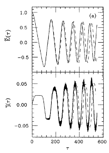
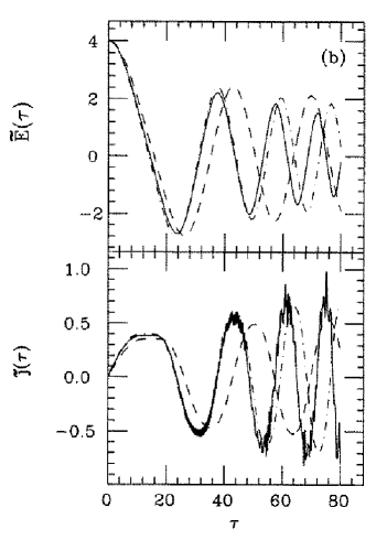
Figure 1: (a) Time evolution of scaled electric field $\tilde{E}$ and current $\tilde{\jmath}$, with initial value $\tilde{E}=1.0$ and coupling $e^{2}/m^{2}=0.1$. Solid line is semiclassical scalar QED, and dashed line is Boltzmann-Vlasov model without the stimulated pair creation correction, Eq. (2.60). (b) Same as (a), but for $\tilde{E}=4.0$. The dashed curve is as in (a), while the dashed-dotted curve includes the correction, Eq. (2.67).

In order to have some insight into these results, we examine an analogous back-reaction problem of a classical system of particles and antiparticles which interact with a homogeneous electric field. For simplicity, we assume that the momentum distributions $N^{\pm}$ of the particles and the antiparticles are localized at $\pm p^{\prime}$,

$$N^{\pm}(p,x)=2\pi\delta(p\mp p^{\prime})n\ ,$$ (2.44)

where $n$ is the density of particles and $p$ is the kinetic momentum. The set of coupled equations for this system reads

$$\ddot{A} = j=2env=2en\frac{p}{\sqrt{p^{2}+m^{2}}}$$

$$\dot{p} = eE=-e\dot{A}\ ,$$ (2.45)

where

$$p=\gamma mv,\quad\gamma=(1-{v}^{2})^{-1/2}.$$ (2.46)

The factor 2 in the current accounts for the antiparticles. This system has an integral of motion from energy conservation,

$$\epsilon=\frac{1}{2}E^{2}+2n\sqrt{p^{2}+m^{2}}$$ (2.47)

and thus

$$\epsilon=\frac{\dot{p}^{2}}{2e^{2}}+2n\sqrt{p^{2}+m^{2}}\ ,$$ (2.48)

where $\epsilon$ is a constant. The last equation is equivalent to the system (2.45), and it reduces the system to the single equation

$$\frac{dp}{dt}=\left(2e^{2}\epsilon-4ne^{2}\sqrt{p^{2}+m^{2}}\right)^{1/2}.$$ (2.49)

The solution of this equation is oscillatory with period

$$T=4\int_{0}^{p_{\rm max}}\frac{dp}{\left(2e^{2}\epsilon-4ne^{2}\sqrt{p^{2}+m^{2}}\right)^{1/2}}\ .$$ (2.50)

Here $p_{\rm max}$ is defined by the zero of the denominator. In the case of a strong initial electric field, the particles and antiparticles are accelerated until they approach the velocity of light. At this point the electric current stops increasing, and the electric field degrades until it changes its direction and accelerates the particles in the opposite direction. If the initial field is very intense, then most of the time the field is strong enough to keep the particles flowing almost at the speed of light. In this case we are able to estimate the period $T$, since the particles are ultrarelativistic. In this limit $p^{2}\gg m^{2}$ and therefore (2.50) yields

$$T_{\it UR}=\frac{2\sqrt{nm+E^{2}_{\rm max}}}{ne}\ ,$$ (2.51)

where $E_{\rm max}$ is the amplitude of the electric field. The current saturates at

$$|j^{\rm max}_{\it UR}|=2en|v^{\rm max}|=2en\ .$$ (2.52)

If the initial electric field is weak, the problem becomes nonrelativistic and the set (2.45) is reduced to a simple harmonic oscillator equation with a frequency

$$\omega^{2}_{p}=\frac{2ne^{2}}{m}\,,\quad T_{\it NR}=\frac{2\pi}{e}\sqrt{\frac{m}{2n}}\ .$$ (2.53)

This is the well-known nonrelativistic plasma frequency. It is evident that for a fixed particle density $n$, the plasma frequency decreases as the electric field increases.

The saturation of the first oscillation in our calculation is thus easy to understand. At the very beginning of the evolution, particles and antiparticles are created and accelerated by the electric field. The current $j$ saturates as $v$ is driven to the speed of light. Eq. (2.52) gives us a method for estimating the number of pairs $n$ created in the first rise of $j$, allowing us to evade the ambiguities in the definition of particle number inherent in the adiabatic approach. We display a graph of the peak current in the first oscillation as a function of the initial field in Fig. 2.

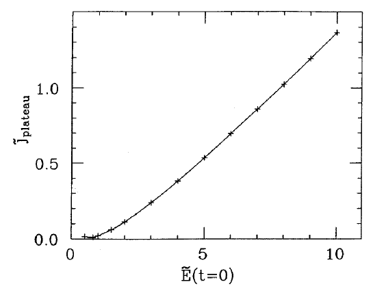
Figure 2: Scaled current $\tilde{\jmath}$ at the peak of the first oscillation, as a function of the initial scaled electric field $\tilde{E}$.

In subsequent oscillations, $n$ is larger and the peak value of $E$ is weaker because of particle production, so the particles remain nonrelativistic even at the peak of the current. At late times, when the envelope of the electric field approaches a constant, that is, when further particle production is negligible, one can estimate the number of particles from (2.53).

We can also evaluate the density of particles by calculating the number operator at some late time, with the expectation that at late times the number density is almost conserved. We define the particle number density by expanding the exact bosonic field operator $\Phi$ in terms of the zeroth-order mode functions

$$f_{k}^{(0)}(t)\equiv\frac{1}{\sqrt{2\omega_{\bf k}(t)}}\,\exp\left[-i\int^{t}\omega_{k}(t^{\prime})dt^{\prime}\right]\ .$$ (2.54)

Then the corresponding creation and annihilation operators, $a_{k}^{(0)}$ and $b_{k}^{(0)}$, become time-dependent, and the vacuum expectation value of the number operator

$$n(k;t)\equiv\langle 0|a^{(0)\dagger}_{k}(t)a^{(0)}_{k}(t)|0\rangle$$ (2.55)

may be computed by a Bogolyubov transformation from the basis functions (2.15) to the basis functions (2.54). (See Appendix A for details.) In the limit of large times we define

$$\lim_{t\to\infty}a_{k}^{(0)}(t)\equiv a_{k}^{\rm out}.$$ (2.56)

The expectation value of the number operator for large times reads

$$n(k) = \langle{0|a_{k}^{{\rm out}\dagger}a_{k}^{\rm out}|0}\rangle$$ (2.57)

$$= \lim_{t\to\infty}{1\over 4\Omega_{k}\omega_{k}}\left[(\Omega_{k}-\omega_{k})^{2}+{1\over 4}\left((\dot{\Omega}_{k}/\Omega_{k})-(\dot{\omega}_{k}/\omega_{k})\right)^{2}\right].$$

We plot this quantity in Fig. 3.

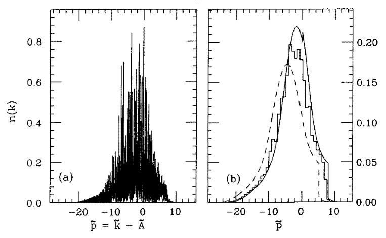
Figure 3: (a) Momentum distribution of produced pairs, for the evolution shown in Fig. 1(a), at time $\tau=550.$ The abscissa is the scaled kinetic momentum $\tilde{p}\equiv\tilde{k}-\tilde{A}$, with $\tilde{k}\equiv k/m$. (b) Data of (a) after smoothing (histogram), compared with Boltzmann-Vlasov model. The smooth curve is for the model with Bose enhancement, the broken curve for the model without.

The rapid oscillations in $n(k)$ are related to rapid oscillations in the integrand in (2.42), which develop with time. From (2.17) we obtain

$$\frac{1}{\Omega_{k}(t)} = \frac{1}{W_{k}(t)}\left[|c_{1k}|^{2}+|c_{2k}|^{2}+c_{1k}^{\ast}c_{2k}\exp{\left(2i\int^{t}W_{k}(t^{\prime})dt^{\prime}\right)}\right.$$ (2.58)

$$+\left.c_{1k}c_{2k}^{\ast}\exp{\left(-2i\int^{t}W_{k}(t^{\prime})dt^{\prime}\right)}\right].$$

Since $W_{k}(t)\simeq\omega_{k}(t)$ in the absence of interaction [see the discussion after Eq. (2.19)], it is evident from (2.58) that for a fixed time, $\Omega_{k}^{-1}$ oscillates as a function of $k$. At a fixed time $t$, this expression oscillates in momentum space with a frequency on the order of $t$. As time goes by, then, the frequency grows, and hence the integrands in the current (2.42) and the particle distribution (2.57) also oscillate. This kind of oscillation appears even if the initial pair-correlation density (related to zitterbewegung [43]) is zero.

When the interaction is switched off, $\dot{\omega}_{k}=0$ but $\dot{\Omega}_{k}\neq 0$. It is clear that in the absence of interaction the expectation value of the number operator should be a constant. One finds that the particle density in (2.57) is indeed time-independent for $\dot{\omega}_{k}=0$ by calculating $\dot{n}(k)$ using (2.16).

2.4 Phenomenological kinetic approach

The simple classical picture presented in the preceding subsection can explain gross features of the time evolution of our system, such as the early saturation of the current and, for that matter, the very existence of plasma oscillations. Particle creation is not included, nor is the distribution of the created particles in momentum. The inclusion of these features requires a more sophisticated model, and a relativistic kinetic equation suggests itself. The original Boltzmann-Vlasov equation, however, conserves particle number, and thus one must add an explicit source term.

Many calculations in the realm of nucleus–nucleus collisions have been based on such a phenomenological model [39–42]. In the case of a homogeneous electric field in 1+1 dimensions, the relativistic kinetic equation is

$$\frac{\partial f}{\partial t}+eE\frac{\partial f}{\partial p}=\frac{dN}{dt\,dx\,dp}\ ,$$ (2.59)

where $f(p,t)$ is the ($x$-independent) classical phase-space distribution, expressed as a function of the kinetic momentum $p$, and the right-hand side is the boson pair-production rate. For the latter, one assumes the applicability of Schwinger’s formula,

$$\frac{dN}{dt\,dx\,dp}={|eE(t)|}\log\left[1+\exp\left(-\frac{\pi m^{2}}{|eE(t)|}\right)\right]\,\delta(p)\ ,$$ (2.60)

despite the fact that here the electric field is not constant in time. The factor $\delta(p)$ indicates the usual WKB assumption that the particles are produced at rest [30]. Initially, $f(p,0)=0$. Eq. (2.59) may be solved using the characteristics ${dp}/{dt}=eE$, giving

$$f(p,t) = \int_{0}^{t}dt^{\prime}\,{|eE(t^{\prime})|}\,\log\left[1+\exp\left(-\frac{\pi m^{2}}{|eE(t^{\prime})|}\right)\right]\,$$ (2.61)

$$\qquad\hbox{}\times\delta\bigl{(}p-eA(t^{\prime})+eA(t)\bigr{)}\ .$$

The $\delta$-function allows us to perform the integration, whence

$$f(p,t)=\sum_{i}\log\left[1+\exp\left(-\frac{\pi m^{2}}{|eE(t_{i})|}\right)\right],$$ (2.62)

where the $t_{i}$’s fulfill $p+eA(t)-eA(t_{i})=0$ and $t_{i}<t$.

The kinetic equation is coupled to the Maxwell equation,

$$\frac{d^{2}\!A}{dt^{2}}=j_{total}=j_{cond}+j_{pol}\ ,$$ (2.63)

where the conduction current is

$$j_{cond}=2e\int\frac{dp}{2\pi}\,\frac{p}{\epsilon_{p}}\,f(p,t)\ ,$$ (2.64)

with $\epsilon_{p}\equiv\sqrt{p^{2}+m^{2}}$, and the polarization current is [42]

$$j_{pol}=\frac{2}{E}\int\frac{dp}{2\pi}\,\epsilon_{p}\frac{dN}{dt\,dx\,dp}\ .$$ (2.65)

[The factors of 2 in (2.64) and (2.65) account for the contributions of the antiparticles.] Inserting (2.61) into (2.63) reduces the system to a single equation,

$$\frac{d^{2}\tilde{A}}{d\tau^{2}} = \frac{e^{2}}{\pi m^{2}}\int_{0}^{\tau}\,d\tau^{\prime}\frac{\tilde{A}(\tau^{\prime})-\tilde{A}(\tau)}{\sqrt{\left[\tilde{A}(\tau^{\prime})-\tilde{A}(\tau)\right]^{2}+1}}\left|\tilde{E}(\tau^{\prime})\right|$$ (2.66)

$$\qquad\mbox{}\times\log\left[1+\exp\left(-\frac{\pi}{\left|\tilde{E}(\tau^{\prime})\right|}\right)\right]$$

$$\mbox{}+\frac{e^{2}}{\pi m^{2}}\,{\rm sign}\left(\tilde{E}(\tau)\right)\log\left[1+\exp\left(-\frac{\pi}{\left|\tilde{E}(\tau)\right|}\right)\right],$$

in terms of the dimensionless variables $\tilde{A}\equiv eA/m$, $\tilde{E}$, and $\tau$.

Equation (2.59), widely used in the literature, omits a statistical factor which should be present. Roughly speaking, the source term should contain the Bose-Einstein factor $\bigl{(}1+f(p,t)\bigr{)}\bigl{(}1+\bar{f}(-p,t)\bigr{)}$, where $\bar{f}$ is the antiparticle density. The $CP$ symmetry of the problem (and of the chosen initial conditions) implies that $\bar{f}(-p,t)=f(p,t)$, and thus the statistical factor is $\bigl{(}1+f(p,t)\bigr{)}^{2}$. Detailed balance, however, dictates that there should be a loss term as well, due to particle annihilation, containing the same matrix element but the statistical factor $f(p,t)\bar{f}(-p,t)=\bigl{(}f(p,t)\bigr{)}^{2}$. The difference of the gain and loss terms is thus proportional to $\bigl{(}1+f(p,t)\bigr{)}^{2}-\bigl{(}f(p,t)\bigr{)}^{2}=1+2f(p,t)$. We thus replace (2.60) with

$$\frac{dN}{dt\,dx\,dp}=\bigl{(}1+2f(p,t)\bigr{)}{|eE(t)|}\log\left[1+\exp\left(-\frac{\pi m^{2}}{|eE(t)|}\right)\right]\,\delta(p)\ .$$ (2.67)

The modifications to (2.61)–(2.62) and (2.66) are obvious. In (2.62), note carefully the strict inequality $t_{i}<t$.

2.5 Comparison in 1+1 dimensions

Let us compare the results of the phenomenological kinetic model with those of our semiclassical analysis. The time evolution of $\tilde{E}$ and $\tilde{\jmath}$ in the kinetic theory is shown in the dashed and dotted curves of Fig. 1, where we see that there is good quantitative agreement between the results obtained with the two very different methods, as long as Bose-Einstein enhancement is properly taken into account. Still, the oscillations are faster and the electric fields decay more rapidly in the quantum calculation than in the Boltzmann-Vlasov model.

The distribution function $f(p,t)$, measured after several plasma oscillations, may be compared with the $n(k)$ of the quantum theory after the latter is smoothed, as shown in Fig. 3. Naturally, the curves have different normalizations and a relative displacement due to the slightly different values of $j$ and $A$. The kinetic theory is quite successful at reproducing the (smoothed) quantum result. One can thus use the kinetic-theory model to explain various features of the particle distribution, such as the sharp edges and tails.

Let us investigate the formal solution given in (2.62). The sum in (2.62) consists of terms for which the following condition is fulfilled:

$$p+eA(t)-eA(t_{i})=0,\quad t_{i}<t.$$ (2.68)

This is represented graphically in Fig. 4.

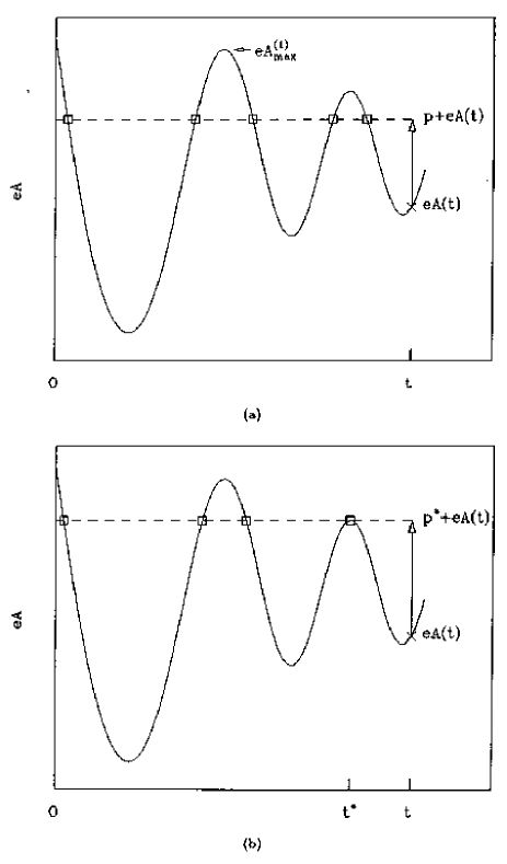
Figure 4: (a) Schematic plot of $A(t)$, showing graphical construction which gives $f(p,t)$ from (2.62). The boxes represent the set of $t_{i}$ corresponding to a given value of $p$, which is the length of the vertical arrow at $t$. We define $A^{(1)}_{\rm max}$ to be the value of $A(t)$ at the highest stationary point. (b) Construction of $f(p,t)$ when $p=p^{*}$, a branch point where terms in (2.62) disappear.

Eq. (2.68) shows that the maximal and minimal values of $A$ at all times up to $t$ determine the highest and lowest momenta in the momentum distribution function, since for $p>eA_{\rm max}-eA(t)$ and for $p<eA_{\rm min}-eA(t)$ there is no solution for $t_{i}$. Now consider Fig. 5.

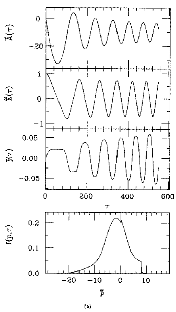
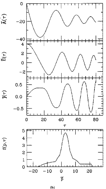
Figure 5: (a) Time evolution of scaled gauge field $\tilde{A}$, electric field $\tilde{E}$, and current $\tilde{\jmath}$ for the Boltzmann-Vlasov model with the stimulated pair creation correction. The initial field is $\tilde{E}=1.0$ and the coupling is $e^{2}/m^{2}=0.1$. Also shown is the momentum distribution $f$ of produced pairs at time $\tau=550$. (b) Same as (a), but for initial $\tilde{E}=4.0$, with $f$ measured at $\tau=80$.

In the case where $\tilde{E}_{\tau=0}=4$ the $\tilde{A}$ field is always negative, never crossing zero after $\tau=0$. By examining Fig. 5(b) we can explain the existence of the plateau on the right-hand side of the distribution function $n(k)$: For momenta in the range $eA^{(1)}_{\rm max}-eA(t)<p<eA(0)-eA(t)$, where $A^{(1)}_{\rm max}$ is defined in Fig. 4, the only contribution to the sum (2.62) results from $t_{i}$ near zero, and the electric field at these early times is changing slowly from its initial value. The momentum distribution drops suddenly to zero at $p=eA(0)-eA(t)$, where the only solution to (2.68) disappears and there are thus no terms in the sum (2.62).

Consider now a generic point $\hat{p}$ in the momentum distribution at time $t$. There are several $t_{i}$’s which fulfill condition (2.68) for $p=\hat{p}$. If we increase $p$, there are branch points $p^{*}$ at which the number of $t_{i}$’s is reduced by two, and therefore there are two fewer terms in the sum (2.62). For these values of $p$, the dashed line in Fig. 4(b) just touches a local extremum of $A$. As $p\to p^{*}$, two of the times $t_{i}$ approach $t^{*}$, the time at the extremum of $A$. Note, now, that $E(t^{*})=-\dot{A}(t^{*})=0$. Terms that have $E(t_{i})=0$ do not contribute to the sum (2.62) and therefore at these branch points in $p$ the distribution is continuous, though its derivative jumps.

There are, however, two special cases. The point $p$ which corresponds to $t_{i}=0$ is one—here, $E(t_{i})$ is the initial value of the electric field, which is nonzero. The momentum distribution is thus always discontinuous at $p=eA(0)-eA(t)$. The right edge of the distribution in Fig. 5(b) is a special case of this; in Fig. 5(a), the discontinuity is at $\tilde{p}\simeq 8$, in the interior of the distribution.

The other special case is $p=0$. Here we have the disappearance of the solution of (2.68) with $t_{i}=t$, at which, again, $E\not=0$. Thus there is always a discontinuity at $p=0$.

In the case of $\tilde{E}(0)=1,$ shown in Fig. 5(a), $A^{(1)}_{\rm max}>A(0)$, and the distribution function does not vanish at the point $p=eA(t_{i}=0)-eA(t)$. Rather it decays smoothly to zero as $p\to eA^{(1)}_{\rm max}-eA(t)$.

We offer a final observation regarding the Bose factor $1+2f$. If the electric field were never to change sign, the factor would have no effect, since new particles are only created at $p=0$, while the old particles have been accelerated by the field. Only if $E$ changes sign do some of the existing particles return to $p=0$ so that $f(p=0)$ is nonzero. Thus the Bose factor is not relevant for the usual case of the Schwinger mechanism in which the electric field is fixed in time.

2.6 Numerical results in 3+1 dimensions

Relation to the flux-tube model

So far we have considered calculations in $1+1$ dimensions. Turning to 3+1 dimensions, let us begin by fixing the parameters and initial conditions so as to correspond to the physical problem of particle creation in the flux tube model [30, 39, 40]. The string tension $\sigma$, interpreted as the energy per unit length stored in the flux tube between quark and antiquark, is given by

$$\sigma=\frac{1}{2}E^{2}A\ ,$$ (2.69)

where $A$ is the cross-sectional area of the flux tube and $E$ is the strength of the longitudinal electric field. Applying Gauss’ Law to the quark at either end of the flux tube, one obtains

$$EA=e,$$ (2.70)

where $e$ is the effective charge of a quark (sweeping non-Abelian features under the rug). The Regge slope gives for the string tension [30] $\sigma\simeq 0.2~{}{\rm GeV}^{2}$. Taking $2.5~{}{\rm GeV}^{-1}$ for the radius of the tube, and using constituent quark masses of $0.35\ {\rm GeV}$, one finds by using (2.69) and (2.70) that the dimensionless field strength in this elementary flux tube is $\tilde{E}=eE/m^{2}\simeq 3$, and the charge is $e\simeq 2.5$. The strength of the chromoelectric field created in high-energy nuclear collisions should be stronger than this, since the sources will be in higher representations of the color group [55, 56]; in our calculations, therefore, we choose initial fields in the range $\tilde{E}=$6–10, with $e^{2}=$4–10.

Numerical results

We solve the system (2.16), (2.31), and (2.36) by using Runge-Kutta along with the iterative scheme described at the end of subsection 2.2. Previous attempts to apply Runge-Kutta to the mode equation have encountered instabilities [58], but we find that the combination of Runge-Kutta with the iterative scheme proves to be stable. Simpson’s rule is used to perform the integration in (2.36) in cylindrical coordinates.

In Fig. 6 we display the dimensionless gauge field

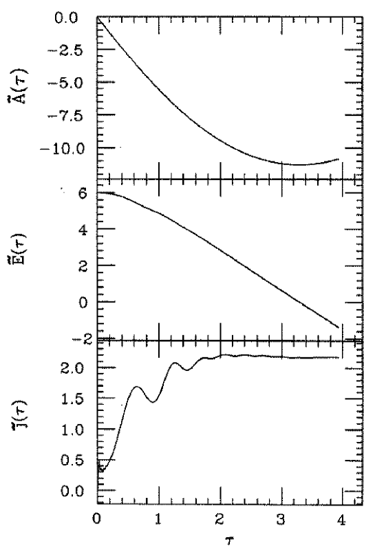
Figure 6: Time evolution of scaled gauge field $\tilde{A}$, electric field $\tilde{E}$, and current $\tilde{\jmath}$ in $3+1$ dimensions, with initial value $\tilde{E}=6.0$ and coupling $e^{2}=10$.

$\tilde{A}$, electric field $\tilde{E}$ , and current $\tilde{\jmath}$ as functions of the dimensionless time $\tau$. We have set $\tilde{E}(0)=6$ and $e^{2}=10$, and measure energy in units of $m$. To get these high-precision results, we used a momentum matrix grid of $200\times 1000$ for transverse and longitudinal momenta, with a time step $d\tau=0.0005$ and momentum intervals $dk_{\parallel}=dk_{\perp}=2\pi/25$. One can see the saturation of the current in the first oscillation, as in 1+1 dimensions. To go to large times, we used smaller momentum grids and larger time steps. For the results shown in Figs. 7 and 8 we

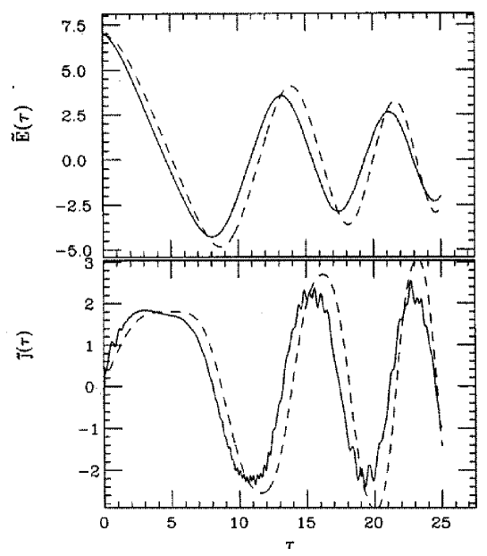
Figure 7: Time evolution of scaled electric field $\tilde{E}$ and current $\tilde{\jmath}$ in $3+1$ dimensions, with initial value $\tilde{E}=7.0$ and coupling $e^{2}=4$. Solid line is semiclassical scalar QED, dashed line is the Boltzmann-Vlasov model with the stimulated pair-creation correction.

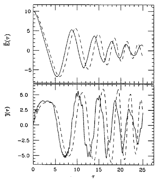
Figure 8: Same as Fig. 7, but for initial $\tilde{E}=10.0$ and $e^{2}=5$.

used momentum grids of $100\times 400$ and $200\times 200$, respectively, and a time step of $d\tau=0.005$, with momentum intervals as in the case shown in Fig. 6. Here we can see plasma oscillations.

In order to compare the semiclassical calculation to the phenomenological model, we simply change $m^{2}$ to $m^{2}_{\perp}\equiv m^{2}+k_{\perp}^{2}$ in (2.59)–(2.62) and change the phase space in (2.64)–(2.65) to $d^{3}{\bf p}/(2\pi)^{3}$. The result in $3+1$ dimensions corresponding to (2.66) is

$$\frac{d^{2}\tilde{A}}{d\tau^{2}} = \frac{e^{2}}{4\pi^{3}}\int_{0}^{\tau}\,d\tau^{\prime}\int d^{2}\tilde{p}_{\perp}\left(2f(\tilde{p}_{\parallel}=0,\tilde{\bf p}_{\perp},\tau^{\prime})+1\right)$$ (2.71)

$$\qquad\mbox{}\times\frac{\tilde{A}(\tau^{\prime})-\tilde{A}(\tau)}{\sqrt{\left[\tilde{A}(\tau^{\prime})-\tilde{A}(\tau)\right]^{2}+\tilde{\bf p}_{\perp}^{2}+1}}\left|\tilde{E}(\tau^{\prime})\right|$$

$$\qquad\mbox{}\times\log\left[1+\exp\left(-\frac{\pi(1+\tilde{\bf p}_{\perp}^{2})}{\left|\tilde{E}(\tau^{\prime})\right|}\right)\right]$$

$$+\frac{e^{2}}{4\pi^{3}}\,{\rm sign}\left(\tilde{E}(\tau)\right)\int d^{2}\tilde{p}_{\perp}\sqrt{1+\tilde{\bf p}_{\perp}^{2}}\left(2f(\tilde{p}_{\parallel}=0,\tilde{\bf p}_{\perp},\tau)+1\right)$$

$$\qquad\mbox{}\times\log\left[1+\exp\left(-\frac{\pi(1+\tilde{\bf p}_{\perp}^{2})}{\left|\tilde{E}(\tau)\right|}\right)\right],$$

including Bose enhancement; the tilde represents dimensionless variables. In Figs. 7 and 8 it is seen that the phenomenological Boltzmann-Vlasov results agree fairly well with those of semiclassical QED. Still, the quantitative agreement is not as good as in 1+1 dimensions; furthermore, the phenomenological model misses entirely the rapid oscillations superposed on the plasma oscillation in $\tilde{\jmath}(\tau)$.

3 Fermion pair production

3.1 Introduction

We present here the extension of the semiclassical formalism to spin-$\frac{1}{2}$ fields [51]. Again, we are limited to the case of a spatially homogeneous, classical electric field. In the preceding section we showed that the results of our calculations in semiclassical scalar electrodynamics are very similar to those obtained from the phenomenological relativistic Boltzmann-Vlasov equation. It is of interest to see if the same results obtain for fermions which, unlike bosons, possess no classical limit, and for which Pauli blocking, in place of Bose enhancement, implies quite different consequences.

To apply adiabatic regularization to the fermion problem, we shall again need to express the Fourier amplitudes of the field operators in a WKB-like form. This will allow us to isolate the ultraviolet divergences through an adiabatic expansion and to eliminate them through renormalization. The WKB parametrization will turn out to be a bit more complex than that for the bosons. We shall further see that in order to make the current zero in the initial adiabatic vacuum, we shall need to express physical expectation values by averaging over two different complete sets of linearly independent solutions of the Dirac equation. Our initial state is thus a mixed state. In Subsection 3.2 we derive the coupled equations for the fields in the semiclassical limit of QED, and discuss the adiabatic regularization procedure. In Subsection 3.3 we present our numerical results in 1+1 dimensions and compare them with the phenomenological Boltzmann-Vlasov model.

3.2 Fermion QED in the semiclassical mean field approximation

Equations of motion

The lagrangian density for electrodynamics is

$${\cal L}=\bar{\Psi}i\gamma^{\mu}(\partial_{\mu}+ieA_{\mu})\Psi-m\bar{\Psi}\Psi-\frac{1}{4}F_{\mu\nu}F^{\mu\nu},$$ (3.1)

where the metric convention is taken as $(+---)$. We work explicitly in 3+1 dimensions, leaving the case of 1+1 dimensions for later. For the $\gamma$-matrices we use the convention of Bjorken and Drell [59],

$$\begin{array}[]{lr}\gamma^{0}=\left(\begin{array}[]{cc}I&0\\ 0&-I\end{array}\right)\par&\quad\gamma^{i}=\left(\begin{array}[]{cc}0&\sigma^{i}\\ -\sigma^{i}&0\end{array}\right),\par\end{array}\quad i=1,2,3$$ (3.2)

where $I$ is the identity matrix and $\sigma^{i}$ are the Pauli matrices.

Again we quantize only the matter field, while the electromagnetic field is treated classically. The coupled field equations read

$$(i\gamma^{\mu}\partial_{\mu}-e\gamma^{\mu}A_{\mu}-m)\Psi(x)=0$$ (3.3)

and

$$\partial_{\mu}F^{\mu\nu}=\langle j^{\nu}\rangle=\frac{e}{2}\langle[\bar{\Psi},\gamma^{\nu}\Psi]\rangle\ ,$$ (3.4)

where the expectation value is with respect to the initial state of the spinor field. The commutator in the electric current guarantees a zero expectation value for any charge-conjugation eigenstate. Expressing the solution of the Dirac equation as

$$\Psi(x)=(i\gamma^{\mu}\partial_{\mu}-e\gamma^{\mu}A_{\mu}+m)\Phi(x)\ ,$$ (3.5)

and inserting (3.5) into (3.3), it follows that $\Phi$ satisfies the quadratic Dirac equation [60]

$$\left[(i\partial_{\mu}-eA_{\mu})^{2}-\frac{e}{2}\sigma^{\mu\nu}F_{\mu\nu}-m^{2}\right]\Phi(x)=0\ ,$$ (3.6)

where $\Phi$ is a four-component spinor. Here we consider the case where the electric field is spatially homogeneous so that the field strength $F^{\mu\nu}$ depends only on time. Owing to homogeneity, the Maxwell equations (3.4) allow only configurations where $\langle j^{0}\rangle=0$. We again take the electric field to be in the direction of the $z$-axis and choose a gauge such that only $A\equiv A^{3}(t)$ is nonvanishing. Then the second-order Dirac equation becomes

$$\left[\Box+e^{2}A^{2}(t)+2iA(t)\partial_{3}-ie\partial_{0}A(t)\gamma^{0}\gamma^{3}+m^{2}\right]\Phi(x)=0.$$ (3.7)

Consider first the $c$-number Dirac equation corresponding to (3.7). Spatial homogeneity implies that there exist solutions of the form

$$\phi_{{\bf k}s}(x)=e^{i{\bf k\cdot x}}f_{{\bf k}s}(t)\chi_{s},$$ (3.8)

where

$$\begin{array}[]{lr}\chi_{1}=\left(\begin{array}[]{cc}1\\ 0\\ 1\\ 0\end{array}\right),\par&\chi_{2}=\left(\begin{array}[]{cc}0\\ 1\\ 0\\ -1\end{array}\right),\end{array}$$ (3.9)

$$\begin{array}[]{lr}\chi_{3}=\left(\begin{array}[]{cc}1\\ 0\\ -1\\ 0\end{array}\right),\par&\chi_{4}=\left(\begin{array}[]{cc}0\\ 1\\ 0\\ 1\end{array}\right).\par\end{array}$$ (3.10)

These spinors are chosen to be eigenvectors of $\alpha^{3}=\gamma^{0}\gamma^{3}$ in the representation (3.2) for the $\gamma$-matrices—the eigenvalues of $\alpha^{3}$ are $\lambda_{s}=1$ for $s=1,2$ and $\lambda_{s}=-1$ for $s=3,4$. The spinors satisfy the normalization and completeness conditions

$$\sum_{\alpha=1}^{4}(\chi^{{\dagger}}_{r})^{\alpha}(\chi_{s})_{\alpha} = 2\delta_{rs}\ ,$$

$$\sum_{r=1}^{4}(\chi^{{\dagger}}_{r})^{\alpha}(\chi_{r})_{\beta} = 2\delta^{\alpha}_{\ \beta}\ .$$ (3.11)

Substituting (3.8) into (3.7), it follows that the mode functions $f_{{\bf k}s}(t)$ satisfy

$$\frac{d^{2}f_{{\bf k}s}(t)}{dt^{2}}+\left[{\omega_{\bf k}^{2}(t)-i\lambda_{s}e\frac{dA}{dt}}\right]f_{{\bf k}s}(t)=0\ ,$$ (3.12)

with

$$\omega^{2}_{\bf k}(t)\equiv p_{3}^{2}+{\bf k}_{\perp}^{2}+m^{2},\quad{\bf k}_{\perp}^{2}\equiv k_{1}^{2}+k_{2}^{2},\quad p_{i}\equiv k^{i}-eA^{i}(t)\ .$$ (3.13)

Equations (3.12) are second-order differential equations, and therefore for each $s$ there are two independent solutions. Let $f^{+}_{{\bf k}s}$ and $f^{-}_{{\bf k}s}$ be the two independent solutions of (3.12), which become positive- and negative-frequency solutions in the absence of the electric field. Clearly at the moment we have eight different solutions for the second-order equation (3.6), namely, $f^{\pm}_{{\bf k}s}$ for $s=1,2,3,4$. However, the Dirac equation (3.3) has only four independent solutions. If we restrict ourselves to solutions that belong to the set $s=1,2$ or to the set $s=3,4,$ we shall see that from each set one can construct a linearly independent set of solutions of the Dirac equation.

The form introduced in (3.8) allows us to write $\psi$ as

$$\psi_{{\bf k}s}(x)\equiv\hat{D}\phi_{{\bf k}s}(x)\equiv(i\gamma^{0}\partial_{0}+{\gamma}^{i}k_{i}-e\gamma^{3}A_{3}+m)\phi_{{\bf k}s}(x)\ .$$ (3.14)

Explicitly, the two sets of independent solutions of the Dirac equation may be taken to be

$$\psi^{\pm}_{{\bf k}s}=e^{i{\bf{k\cdot x}}}\hat{D}f^{\pm}_{{\bf k}s}\chi_{s}\ ,\quad s=1,2,$$ (3.15)

and

$$\psi^{\pm}_{{\bf k}s}=e^{i{\bf{k\cdot x}}}\hat{D}f^{\pm}_{{\bf k}s}\chi_{s}\ ,\quad s=3,4.$$ (3.16)

Using Eqs. (3.14)–(3.16) we find, for a given ${\bf k},$

$${\psi^{\pm}_{r}}^{\dagger}{\psi^{\pm}_{s}} = {\chi_{r}}^{\dagger}{f_{r}^{\ast\pm}}{\hat{D}}^{\dagger}\hat{D}f_{s}^{\pm}\chi_{s}$$ (3.17)

$$= 2\left\{\omega^{2}_{\bf k}(t){f_{r}^{\ast\pm}}f_{s}^{\pm}+{{\dot{f}}_{r}^{\ast\pm}}\dot{f}_{s}^{\pm}\right.$$

$$\quad\left.-i\lambda_{s}p_{3}\left[{f_{r}^{\ast\pm}}\dot{f}_{s}^{\pm}-{\dot{f}_{r}^{\ast\pm}}f_{s}^{\pm}\right]\right\}\delta_{rs}\ ,$$

where either $r,s=1,2$ or $r,s=3,4$. An exactly analogous formula may be derived for ${\psi^{\pm}_{r}}^{\dagger}{\psi^{\mp}_{s}}$. By differentiating these expressions with respect to time and by using Eq. (3.12), it can be readily verified that these inner products are time-independent. As $t\rightarrow-\infty$ there is no interaction between the fermion field and the electromagnetic field, and we can choose two independent plane-wave solutions for Eq. (3.12),

$$\lim_{t\rightarrow-\infty}f^{\pm}_{{\bf k}s}=c_{s}e^{\mp i\omega_{\bf k}t},$$ (3.18)

where $c_{s}$ are constants. Insertion of these free solutions in the relation for ${\psi^{\pm}_{r}}^{\dagger}{\psi^{\mp}_{s}}$ yields immediately

$${\psi^{\pm}_{r}}^{\dagger}{\psi^{\mp}_{s}}=0\ .$$ (3.19)

Since this result is time-independent, it is valid at any time, and each set $\psi^{\pm}_{s}$, with $s=1,2$ or $s=3,4$, is a complete set of linearly-independent solutions of the Dirac equation. Note that these complete systems are not identical, and orthonormality conditions holds for each set separately. In principle, we need only one of these sets in order to expand the field operator $\Psi$ in terms of single-particle solutions. In order to ensure that, with our initial conditions, the Dirac current vanishes at $t=0$, it is advantageous to use both sets in our calculations.

We now construct the quantized spinor field operator in the form

$$\Psi(x) = \int[d{\bf k}]\sum_{s=1,2}[b_{s}({\bf k}){\psi^{+}_{{\bf k}s}}+d_{s}^{\dagger}({\bf{-k}}){\psi^{-}_{{\bf k}s}}]$$ (3.20)

$$= \int[d{\bf k}]\sum_{s=3,4}[b_{s}({\bf k}){\psi^{+}_{{\bf k}s}}+d_{s}^{\dagger}({\bf{-k}}){\psi^{-}_{{\bf k}s}}]\ ,$$

where the two lines show the field expressed in terms of the two alternative bases. Here $[d{\bf k}]={d^{3}{\bf k}}/{(2\pi)^{3}}$. The fermion fields obey canonical anticommutation relations, $\{\Psi_{\alpha}(t,{\bf{x}}),\Psi^{\dagger}_{\beta}(t,{\bf{y}})\}=\delta^{3}({\bf{x}}-{\bf{y}})\delta_{\alpha\beta}$. The creation and annihilation operators of each set, $r,s=1,2$ or $r,s=3,4,$ obey the standard anticommutation relations,

$$\{b_{r}({\bf k}),b_{s}^{\dagger}({\bf{q}})\}=\{d_{r}({\bf k}),d_{s}^{\dagger}({\bf{q}})\}=(2\pi)^{3}\delta^{3}({\bf k}-{\bf{q}})\delta_{rs}\ ,$$ (3.21)

if we impose the condition

$${\psi^{\pm}_{r}}^{\dagger}{\psi^{\pm}_{s}}=\delta_{rs}\ ,$$ (3.22)

to normalize the mode functions.

We now calculate the expectation value of the electric current. For the sake of simplicity we choose the initial state to be the vacuum annihilated by $b_{r}({\bf k})$ and $d_{r}({\bf k})$. Using the anticommutation relations (3.21) we find

$$\langle 0|j^{3}|0\rangle = \frac{e}{2}\langle 0|[\bar{\Psi},\gamma^{3}\Psi]|0\rangle$$ (3.23)

$$= \frac{e}{2}\int[d{\bf k}]\sum_{s=1,2}\left\{-{\psi^{+}_{{\bf k}s}}^{\dagger}\gamma^{0}\gamma^{3}{\psi^{+}_{{\bf k}s}}+{\psi^{-}_{{\bf k}s}}^{\dagger}\gamma^{0}\gamma^{3}{\psi^{-}_{{\bf k}s}}\right\}.$$

Alternatively,

$$\langle 0|j^{3}|0\rangle=\frac{e}{2}\int[d{\bf k}]\sum_{s=3,4}\left\{-{\psi^{+}_{{\bf k}s}}^{\dagger}\gamma^{0}\gamma^{3}{\psi^{+}_{{\bf k}s}}+{\psi^{-}_{{\bf k}s}}^{\dagger}\gamma^{0}\gamma^{3}{\psi^{-}_{{\bf k}s}}\right\}.$$ (3.24)

Averaging the two expressions,

$$\langle 0|j^{3}|0\rangle=\frac{e}{4}\int[d{\bf k}]\sum_{s=1}^{4}\left\{-{\psi^{+}_{{\bf k}s}}^{\dagger}\gamma^{0}\gamma^{3}{\psi^{+}_{{\bf k}s}}+{\psi^{-}_{{\bf k}s}}^{\dagger}\gamma^{0}\gamma^{3}{\psi^{-}_{{\bf k}s}}\right\}.$$ (3.25)

This form will be useful when we turn to the adiabatic regularization of the current. The other components of the current are zero since the electric field is in the $z$-direction. Using (3.14) we find

$$\gamma^{0}\gamma^{3}{\psi^{\pm}_{{\bf k}s}}=\lambda_{s}\left[-i\gamma^{0}\partial_{0}+{\bf{\gamma}}^{\perp}{\bf k}_{\perp}-(k_{3}-eA_{3})\gamma^{3}+m\right]{\phi^{\pm}_{{\bf k}s}},$$ (3.26)

and thus (3.17) and (3.22) give

$${\psi^{\pm}_{{\bf k}s}}^{\dagger}\gamma^{0}\gamma^{3}{\psi^{\pm}_{{\bf k}s}}=\chi_{s}^{\dagger}f_{{\bf k}s}^{\ast\pm}{\hat{D}}^{\dagger}\gamma^{0}\gamma^{3}\hat{D}f_{{\bf k}s}^{\pm}\chi_{s}=$$ (3.27)

$$= 2\lambda_{s}\left\{(k^{2}_{\perp}+m^{2}-p_{3}{{}^{2}})f_{{\bf k}s}^{\ast\pm}f_{{\bf k}s}^{\pm}-\dot{f}_{{\bf k}s}^{\ast\pm}\dot{f}_{{\bf k}s}^{\pm}+i\lambda_{s}p_{3}(f_{{\bf k}s}^{\ast\pm}\dot{f}_{{\bf k}s}^{\pm}-\dot{f}_{{\bf k}s}^{\ast\pm}f_{{\bf k}s}^{\pm})\right\}$$

$$= \lambda_{s}\left[4(k^{2}_{\perp}+m^{2})|f_{{\bf k}s}^{\pm}|^{2}-1\right],$$

where the index $s$ is not summed over. Inserting (3.27) into (3.25) yields

$$\langle 0|j^{3}|0\rangle=e\sum_{s=1}^{4}\int[d{\bf k}](k^{2}_{\perp}+m^{2})\lambda_{s}\left(|f_{{\bf k}s}^{-}|^{2}-|f_{{\bf k}s}^{+}|^{2}\right).$$ (3.28)

From (3.17) and (3.22) it can be shown [60] that

$$2(k^{2}_{\perp}+m^{2})\left(|f_{{\bf k}s}^{+}|^{2}+|f_{{\bf k}s}^{-}|^{2}\right)=1.$$ (3.29)

Eq. (3.29) then gives the current as

$$\langle 0|j^{3}|0\rangle=-2e\sum_{s=1}^{4}\int[d{\bf k}](k^{2}_{\perp}+m^{2})\lambda_{s}|f_{{\bf k}s}^{+}|^{2}.$$ (3.30)

Averaging the current expectation value over the two bases as in (3.25) means that we prepare the initial system in a mixed state.

Adiabatic regularization

As in the boson case of the previous section, the difficulty in solving the coupled semiclassical equations (3.3) and (3.4) originates from the fact that the expectation value of the current (3.30) diverges in the interacting theory. This infinity can, as before, be removed by charge renormalization. In order to isolate the ultraviolet behavior of the current integrand by adiabatic expansion, we need to express the mode equations (3.12) in a WKB-like form. The generic problem is to find a suitable parametrization for the solution of the differential equation $\ddot{u}(t)+\epsilon(t)u(t)=0$, where in the present case $\epsilon$ is the complex quantity in square brackets in (3.12). Such a parametrization is found in [57], namely,

$$f_{{\bf k}s}^{+}(t)=N_{{\bf k}s}\frac{1}{\sqrt{2\Omega_{{\bf k}s}}}\exp\left\{\int_{0}^{t}\left(-i\Omega_{{\bf k}s}(t^{\prime})-\lambda_{s}\frac{e\dot{A}(t^{\prime})}{2\Omega_{{\bf k}s}(t^{\prime})}\right)dt^{\prime}\right\},$$ (3.31)

where $N_{{\bf k}s}$ are normalization constants and $\Omega_{{\bf k}s}$ is a real generalized frequency. By substituting (3.31) into (3.12) we obtain the WKB-like equation for $\Omega_{{\bf k}s}$,

$$\Omega^{2}_{{\bf k}s}(t)=-\frac{\ddot{\Omega}_{{\bf k}s}}{2\Omega_{{\bf k}s}}+\frac{3}{4}\frac{\dot{\Omega}^{2}_{{\bf k}s}}{\Omega^{2}_{{\bf k}s}}+\omega^{2}_{\bf k}+\left(\frac{e\dot{A}}{2\Omega_{{\bf k}s}}\right)^{2}-\lambda_{s}\frac{e\ddot{A}}{2\Omega_{{\bf k}s}}+\lambda_{s}\frac{e\dot{A}\dot{\Omega}_{{\bf k}s}}{\Omega^{2}_{{\bf k}s}}.$$ (3.32)

As in the boson case, the equation for $\Omega$ is a second-order nonlinear differential equation.

This equation enables us to study the large-momentum behavior of the solutions. As above, an adiabatic expansion of (3.32) to second order is needed to identify the divergences in the current (3.30). Noting that

$$\ddot{\omega}_{\bf k}=\frac{-e\ddot{A}p_{3}}{\omega_{\bf k}}+O(1/\omega_{\bf k}),$$ (3.33)

we have up to second order [i.e., iterating (3.32) once]

$$\Omega_{{\bf k}s}=\omega_{\bf k}-e\ddot{A}\left(\lambda_{s}\omega_{\bf k}-p_{3}\right)/4\omega^{3}_{\bf k}+O(1/\omega^{3}_{\bf k}).$$ (3.34)

Using the ansatz (3.31) the current reads

$$\langle 0|j^{3}|0\rangle=-2e\sum_{s=1}^{4}\int[d{\bf k}](k^{2}_{\perp}+m^{2})\lambda_{s}\left[\frac{|N_{{\bf k}s}|^{2}}{2\Omega_{{\bf k}s}}\exp\left\{-\lambda_{s}\int\frac{e\dot{A}(t^{\prime})}{\Omega_{{\bf k}s}(t^{\prime})}dt^{\prime}\right\}\right].$$

(3.35)

Equations (3.17) and (3.22) determine the normalization constants, and it turns out that the expression in square brackets is

$$\frac{|N_{{\bf k}s}|^{2}}{\Omega_{{\bf k}s}}\exp\left\{-\lambda_{s}\int\frac{e\dot{A}(t^{\prime})}{\Omega_{{\bf k}s}(t^{\prime})}dt^{\prime}\right\} = \left[\omega^{2}_{\bf k}+\left(\frac{-\lambda_{s}e\dot{A}}{2\Omega_{{\bf k}s}}-\frac{\dot{\Omega}_{{\bf k}s}}{2\Omega_{{\bf k}s}}\right)^{2}+\Omega^{2}_{{\bf k}s}\right.$$ (3.36)

$$\mbox{}-\lambda_{s}2p_{3}\Omega_{{\bf k}s}\Biggr{]}^{-1}$$

$$\equiv \Gamma_{{s}}({\bf k})\ .$$

With the identity

$$k^{2}_{\perp}+m^{2}=[\omega_{\bf k}+p_{3}][\omega_{\bf k}-p_{3}],$$ (3.37)

we obtain

$$\langle 0|j^{3}|0\rangle = e\int{[d{\bf k}]}\left\{\frac{\omega_{\bf k}-p_{3}}{\omega_{\bf k}+e\ddot{A}(\omega_{\bf k}+p_{3})/4\omega^{3}_{\bf k}}-\frac{\omega_{\bf k}+p_{3}}{\omega_{\bf k}-e\ddot{A}(\omega_{\bf k}-p_{3})/4\omega^{3}_{\bf k}}\right.$$ (3.38)

$$+\,O(\omega^{-4}_{\bf k})\biggr{\}}.$$

At large momentum, we approximate

$$\frac{1}{1\pm e\ddot{A}[\omega_{\bf k}\pm p_{3}]/4\omega^{4}_{\bf k}}\simeq 1\mp\frac{e\ddot{A}}{4\omega^{4}_{\bf k}}[\omega_{\bf k}\pm p_{3}]\ .$$ (3.39)

After we perform the angular integrations and drop terms that are odd functions of $p_{3}$, the Maxwell equation becomes

$$\ddot{A} = \langle 0|j^{3}|0\rangle={-e^{2}\ddot{A}}\int[d{\bf k}]\left(\frac{1}{2\omega^{3}_{\bf k}}-\frac{p_{3}^{2}}{2\omega^{5}_{\bf k}}\right)+({\rm finite\;part})$$ (3.40)

$$= {-e^{2}\ddot{A}}\,\delta e^{2}+({\rm finite\;part}),$$

where

$$\delta e^{2}\equiv\int[d{\bf k}]\left(\frac{1}{2\omega^{3}_{\bf k}}-\frac{p_{3}^{2}}{2\omega^{5}_{\bf k}}\right)=\frac{1}{4\pi^{2}}\int_{0}^{\infty}dk\left[\frac{k^{2}}{(k^{2}+m^{2})^{\frac{3}{2}}}-\frac{k^{4}}{3(k^{2}+m^{2})^{\frac{5}{2}}}\right].$$ (3.41)

The current in (3.40) diverges logarithmically, with the same divergence as the vacuum polarization $\Pi(q^{2}=0)$. Renormalizing as usual, we define

$$e^{2}_{R}=e^{2}(1+e^{2}\delta e^{2})^{-1}\equiv Ze^{2},\quad\quad A_{R}=Z^{-1/2}A,$$ (3.42)

so that $eA=e_{R}A_{R}$. We can also write $Z=(1-e^{2}_{R}\delta e^{2})$. Multiplying (3.35) by $Ze/e_{R}$ we obtain

$$\ddot{A}_{R}-e^{2}_{R}\ddot{A}_{R}\delta e^{2}=e_{R}\sum_{s=1}^{4}\int[d{\bf k}](k^{2}_{\perp}+m^{2})(-\lambda_{s})\Gamma_{s}({\bf k})\ .$$ (3.43)

Using (3.41) and rearranging, we have

$$\ddot{A}_{R}=e_{R}\int[d{\bf k}]\left[(k^{2}_{\perp}+m^{2})\sum_{s=1}^{4}(-\lambda_{s})\Gamma_{s}({\bf k})+{e_{R}^{2}\ddot{A_{R}}}\left(\frac{1}{2\omega^{3}_{\bf k}}-\frac{p_{3}^{2}}{2\omega^{5}_{\bf k}}\right)\right],$$ (3.44)

where the right-hand side is finite. We drop the $R$ subscripts now.

As for the boson problem, we can define a remainder which is the difference between the integrand in (3.35) and its adiabatic approximation. Examining (3.38), (3.39), and (3.43), we can write

$$(k^{2}_{\perp}+m^{2})\sum_{s=1}^{4}(-\lambda_{s})\Gamma_{s}({\bf k})=-\frac{2p_{3}}{\omega_{\bf k}}-\frac{e\ddot{A}}{2\omega^{5}_{\bf k}}(\omega^{2}_{\bf k}-\pi^{2}_{3})+R_{\bf k}(t)\ .$$ (3.45)

At large momentum this minimal adiabatic approximation matches the exact integrand up to terms that fall off as $O(1/\omega^{3}_{\bf k})$, so the remainder $R_{\bf k}(t)$ falls off faster. Upon substituting (3.45) into (3.44) and using (3.38)–(3.40), the finite Maxwell equation takes the form

$$\ddot{A}=e\int[d{\bf k}]R_{\bf k}(t).$$ (3.46)

Again, the subsidiary condition (3.45) defining $R_{\bf k}$ is an intrinsic part of (3.46).

As in the boson case, the initial conditions we impose are

$$\dot{A}(t=0)=-E_{0}\,,\quad A(t=0)=0\,,$$ (3.47)

and

$$\Omega_{{\bf k}s}(t=0)=\omega_{{\bf k}}(t=0)\,,\quad\dot{\Omega}_{{\bf k}s}(t=0)=\dot{\omega}_{{\bf k}}(t=0)\,,$$ (3.48)

which specifies the adiabatic vacuum. Nonvacuum initial conditions may be handled in a manner analogous to the bosonic case by adding nonzero particle number densities to the current expectation value.

Here, too, the choice of initial conditions is constrained by demanding the consistency of the adiabatic expansion (3.45) with the Maxwell equation (3.46). By substituting (3.48) into (3.36) and (3.45) we find that $\ddot{A}(0)=0$, but

$$R_{\bf k}(0)=\frac{2p_{3}}{\omega_{\bf k}}\left\{1-\frac{1+e^{2}E^{2}_{0}/4\omega^{4}_{\bf k}}{\left[(1+e^{2}E^{2}_{0}/8\omega^{4}_{\bf k})^{2}-(e^{2}E^{2}_{0}p_{3}/8\omega^{5}_{\bf k})^{2}\right]}\right\}$$ (3.49)

is not zero. It turns out, however, that the integration over $\bf k$ in (3.46) gives zero by charge conjugation symmetry $p_{3}\rightarrow-p_{3}$. Thus the initial conditions (3.47) and (3.48) are consistent with the requirements of renormalization. We emphasize that choosing $R_{\bf k}(0)=0$ is not consistent with the initial conditions (3.48).

Given such a set of consistent initial conditions, we can solve the back-reaction equations (3.32), (3.45), and (3.46) exactly as we did in the scalar case. To do this we take $R_{\bf k}$ to be zero at an extremely large momentum as a trial value, so that $\ddot{A}$ can be extracted from (3.45). Now having $\ddot{A}$, we use (3.45) to extract $R_{\bf k}$ for each ${\bf k}$ up to this very large momentum. Then, substituting $R_{\bf k}$ in (3.46) we get a new corrected value for $\ddot{A}$. This procedure may be iterated until convergence for $\ddot{A}$ and $R_{\bf k}$ is reached, after which one may proceed to the next time step.

3.3 Calculation in 1+1 dimensions

Dynamical equations

For the fermion problem, we present numerical results only for the (1+1)-dimensional case. Let us indicate the modifications needed in the equations. The $\gamma$-matrices are given by

$$\begin{array}[]{lr}\gamma^{0}=\left(\begin{array}[]{cc}1&0\\ 0&-1\end{array}\right),\par&\gamma^{1}=\left(\begin{array}[]{cc}0&1\\ -1&0\end{array}\right),\par\end{array}$$ (3.50)

and $\gamma^{1}$ plays the role that $\gamma^{3}$ played in the (3+1)-dimensional case. In $A^{0}=0$ gauge, we define $A^{1}=A(t)$, and the second-order Dirac equation is

$$\left[\Box+e^{2}A^{2}(t)+2iA(t)\partial_{1}-ie\partial_{0}A(t)\gamma^{0}\gamma^{1}+m^{2}\right]\phi(x)=0.$$ (3.51)

The Dirac equation in two dimensions has two independent solutions: Either

$$f_{k1}^{+}\chi_{1}\,,\quad f_{k1}^{-}\chi_{1}\quad$$ (3.52)

or

$$f_{k2}^{+}\chi_{2}\,,\quad f_{k2}^{-}\chi_{2}$$ (3.53)

may be taken as the basis set of independent solutions. Here $\gamma^{0}\gamma^{1}\chi_{{s}}=\lambda_{s}\chi_{{s}}$ with $\lambda_{1}=1$ and $\lambda_{2}=-1$, and the spinors $\chi_{{s}}$ are given by

$$\begin{array}[]{lr}\chi_{1}=\left(\begin{array}[]{cc}1\\ 1\end{array}\right),\par&\chi_{2}=\left(\begin{array}[]{cc}1\\ -1\end{array}\right).\end{array}$$ (3.54)

We define

$$\omega^{2}_{k}(t)\equiv p^{2}+m^{2},\quad p\equiv k-eA^{1}(t)\ .$$ (3.55)

The Maxwell equation is

$$\ddot{A}=\langle 0|j^{1}|0\rangle=2e\int\frac{dk}{2\pi}m^{2}\{|f_{k2}^{+}|^{2}-|f_{k1}^{+}|^{2}\}.$$ (3.56)

In two dimensions there is no spin, and thus there are half as many terms as in (3.30) after summation.

Renormalization of (3.56) can be done in the same way as in subsection 3.3. In two-dimensional QED the charge renormalization is finite and we find that $\delta e^{2}=(6\pi m^{2})^{-1}$. Therefore, in the renormalized Maxwell equation, $\ddot{A}$ can be isolated [in contrast to (3.44)], and we obtain

$$\ddot{A}_{R}=\frac{e_{R}}{1-e^{2}_{R}\delta e^{2}}\int\frac{dk}{2\pi}\left\{m^{2}\sum_{s=1,2}\left(-\lambda_{s}\Gamma_{s}(k)\right)+2\frac{p}{\omega_{k}}\right\}$$ (3.57)

where

$$\Gamma_{{s}}(k)\equiv\left[\omega^{2}_{k}+\left(\frac{-\lambda_{s}e_{R}\dot{A}_{R}}{2\Omega_{ks}}-\frac{\dot{\Omega}_{ks}}{2\Omega_{ks}}\right)^{2}+\Omega^{2}_{ks}-\lambda_{s}2p\Omega_{ks}\right]^{-1}.$$ (3.58)

The last term in the braces in (3.57) does not contribute to the integral but was included for numerical purposes. The set of equations (3.32) and (3.57) with the initial conditions (3.47) and (3.49) defines the numerical back-reaction problem.

Numerical results

We show in Figs. 9 and 10 the time evolution of the

Figure 9: Fermion pair creation in 1+1 dimensions: Time evolution of the scaled electric field $\tilde{E}$ and current $\tilde{\jmath}$, with initial value $\tilde{E}=1.0$ and coupling $e^{2}/m^{2}=0.1$. Solid line is semiclassical QED, and dashed line is Boltzmann-Vlasov model.

Figure 10: As in Fig. 9, but for initial field $\tilde{E}=4.0$.

scaled electric field $\tilde{E}\equiv eE/m^{2}$ and the induced current $\tilde{\jmath}\equiv ej/m^{3}$ as functions of $\tau\equiv mt$. Here we used a time step of $d\tau=5\times 10^{-4}$ and a momentum grid with $d\tilde{k}\equiv dk/m=0.003$. The results are similar to those for bosons, with initial particle creation followed by plasma oscillations. In this case the current saturates twice in the early stages of evolution, each time because the particle velocity approaches $c$, with more particles present (and hence a larger current) in the second instance.

The amplitude of the electric-field oscillations decreases substantially only in the first few oscillations and remains almost constant at later times. This means that essentially all of the pair production happens in the first oscillations. One sees that in successive oscillations $n$ is larger and $E$ is weaker, and therefore the frequency of oscillations increases. As we have noted, the frequency of relativistic plasma oscillations depends not only on $n$ but also on the amplitude of $E$: The weaker the field the higher the frequency, in contrast to the nonrelativistic case where the plasma frequency does not depend on the amplitude.

We display in Figs. 11(a) and 12(a) the momentum distribution

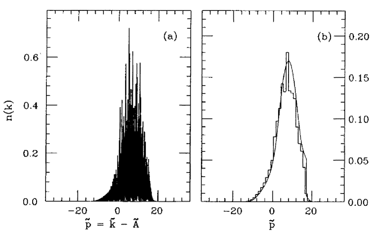
Figure 11: (a) Momentum distribution of produced pairs, for the evolution shown in Fig. 9, at time $\tau=600.$ The abscissa is the scaled kinetic momentum $\tilde{p}\equiv\tilde{k}-\tilde{A}$, with $\tilde{k}\equiv k/m$. (b) Data of (a) after binning (histogram), compared with Boltzmann-Vlasov model (curve).

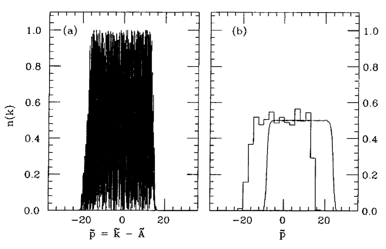
Figure 12: The same as Fig. 11, but for the evolution shown in Fig. 10 (i.e., initial field $\tilde{E}=4.0$), at time $\tau=200.$

of the produced particles, defined by

$$n(k;t)\equiv\frac{1}{2}\sum_{s=1,2}\left\langle 0\left|b^{(0)\dagger}_{s}({\bf k};t)b^{(0)}_{s}({\bf k};t)\right|0\right\rangle\ .$$ (3.59)

In accordance with the Pauli principle, the occupation number does not exceed one.

Phenomenological transport equations

The fermionic counterpart of (2.67) is

$$\frac{\partial f}{\partial t}+eE\frac{\partial f}{\partial p} = \frac{dN}{dt\,dx\,dp}$$ (3.60)

$$= -\bigl{(}1-2f(p,t)\bigr{)}|eE(t)|$$

$$\quad\mbox{}\times\log\left[1-\exp\left(-\frac{\pi m^{2}}{|eE(t)|}\right)\right]\,\delta(p).$$

Recall that $p$ is the kinetic momentum. The right-hand side is the Schwinger expression for the fermion pair-production rate in 1+1 dimensions, multiplied by the statistical factor $(1-2f)$ which represents Pauli blocking and detailed balance (see the brief discussion above Eq. (2.67)).

Note that the singularity on the right-hand side of (3.60) for $m=0$ is spurious. The Schwinger formula is based on a tunneling picture [30] that incorporates conservation of energy, but ignores other conservation rules that would follow from specific features of the system in question. In the present case, where dynamical photons are absent, chirality conservation actually forbids pair production from the homogeneous electric field for massless particles in one spatial dimension, so that the use of the Schwinger formula is unjustified in this limit. In the field theory, however, there is no such limitation. The $m\to 0$ limit is nothing other than the Schwinger model [28, 61], and the chiral anomaly gives a finite rate [28, 62] for pair production.

Eq. (3.60) is solved in the same way as (2.67). The time evolutions of the scaled field strength $\tilde{E}$ and current $\tilde{\jmath}$ are shown in the dashed curves of Figs. 9 and 10. The quantitative agreement between the kinetic theory and the quantum theory is striking. The amplitude of the electric field approaches a limiting value after a few oscillations, meaning that thereafter the production of particles is negligible. In the boson case an analogous effect is seen, but it sets in somewhat later than for fermions. The constant amplitude reflects the absence of pair creation from virtual photons and the exponentially small spontaneous pair creation rate at this stage of the evolution. The fact that the electric field reaches its limiting value more quickly for fermions than for bosons may be due to the difficulty of producing more fermions once the low-momentum states have been occupied.

The comparison between $f(p,t)$ at a late time and the smoothed $n(k)$ of the quantum theory is shown in Figs. 11(b) and 12(b). The importance of Pauli blocking is obvious. Without the statistical factor in (3.60) the occupation number exceeds one if the initial electric field is strong enough [51]. The Schwinger source term in (3.60) is very large for a strong electric field; it is the $(1-2f)$ term that prevents the violation of the Pauli principle.

As for the boson case, our comparison provides a justification for using the kinetic theory in studying the quark-gluon plasma. Past treatments have not, however, included the Pauli-blocking term which is crucial for strong fields.

4 Concluding remarks

We have solved semiclassical QED for strong fields using the adiabatic regularization method for spatially-homogeneous electric fields. We determine initial values of the fields and their derivatives which are consistent both with the coupled Maxwell and matter-field equations and with the adiabatic regularization scheme. This is a nonperturbative calculation, which enables us to investigate the dynamical evolution of the interacting system of matter and the electromagnetic field. Careful computational work was essential in order to achieve numerical stability for this system since it consists of three time scales which are related to frequencies of the order of the mass of the produced particles (short time scale), the plasma oscillations of the electric field and current (medium time scale), and the degradation of the electric field to small values, by which point particle production is negligible (long time scale). It requires fine grids in momentum space and small time steps to solve the differential equations.

Physical features like plasma oscillations and the plateau in the first period of the current evolution are understood by solving a classical relativistic system of particles in the presence of an electric field. From the value of the plasma oscillation frequency or the height of the first plateau of the current we obtain two separate estimates of the number of particles at the corresponding times.

There is agreement between QED and a simple phenomenological model based on classical Boltzmann-Vlasov equations supplemented with a Schwinger WKB formula. This agreement is significantly improved when the source term is multiplied by a Pauli-blocking or Bose-enhancement factor. The phenomenological model enables us to obtain immediate physical insight and allows us perform calculations that are much faster and easier than those of the full QED formulation. In addition in the phenomenological model we understand the meaning of the number of particles, whereas in QED this concept is ill-defined as long as the interaction takes place. The agreement between the number of particles in these two calculations then allows us to assess the quality of the definition of the number of particles in the field theory in the presence of interaction.

The existence of a phenomenological model, in this simplified situation, with physical and numerical content very close to that of the exact field-theory treatment opens the way for studies that include spatial dependence, real radiation, and, eventually, color degrees of freedom. At the same time, it suggests that further application of phenomenological transport equations for systems involving pair production is in order.

Acknowledgements

Major progress on this subject was made during visits of Y.K. and B.S. to the Theory Division at the Los Alamos National Laboratory. We are very grateful for having had the opportunity to work there with F. Cooper and E. Mottola. Their willingness to collaborate and to share their physical insight aided this work substantially. The hospitality of the Theoretical Division at Los Alamos National Laboratory during these visits is also greatly appreciated, as is the access the Division provided to computing facilities there.

We wish to thank I. Paziashvili for many enlightening discussions, as well as A. Casher, M.S. Marinov, S. Nussinov, N. Weiss, and S. Yankielowicz for valuable help.

Thanks are due to the German-Israel Foundation, the Minerva Foundation, the Alexander von Humboldt-Stiftung, and the Yuval Ne’eman Chair in Theoretical Nuclear Physics at Tel Aviv University for partial support of this work. The work of B.S. was partially supported by a Wolfson Research Award administered by the Israel Academy of Sciences and Humanities. Part of this work was carried out while J.M.E. was visiting the Institut für Theoretische Physik der Universität Frankfurt, to whom he is grateful for their warm hospitality.

Appendix: Particle spectra

During the process of particle production, the particle number is not conserved, and we are not in an out-state region. However, it is possible to introduce an interpolating particle number operator, using the time-dependent creation and annihilation operators of the first-order adiabatic vacuum. This interpolating number operator has the property that if at $t=0$ the initial state is equal to the first-order adiabatic vacuum state, then the number operator starts at zero. At late times, the first-order adiabatic number operator approaches the usual out-state number operator.

The wave functions of the first-order adiabatic expansion,

$$\phi^{(0)}_{\bf{k}}({\bf{x}},t) = e^{i{{\bf{k}}\cdot{\bf{x}}}}f^{(0)}_{\bf{k}}(t),$$

$$f^{(0)}_{\bf{k}}(t) = {{e^{-i\int_{0}^{t}\omega_{\bf{k}}(t^{\prime})dt^{\prime}}}\over{(2\omega_{\bf{k}}(t))^{1/2}}}={e^{-iy^{(0)}_{\bf{k}}(t)}\over{(2\omega_{\bf{k}}(t))^{1/2}}},$$

$$\bar{\phi}^{\ast(0)}_{\bf{k}}({\bf{x}},t) = f_{-{\bf{k}}}^{\ast(0)}(t)e^{-i{\bf{k}}\cdot{\bf{x}}},$$ (A.1)

form an alternative basis for expanding the quantum field $\Phi$, so that we can write

$$\Phi(t,z,{\bf{x}}_{\perp})=\int[d{\bf{k}}]\left(a_{\bf{k}}(t)\phi^{(0)}_{\bf{k}}({\bf{x}},t)+b^{\dagger}_{\bf{k}}(t)\bar{\phi}^{\ast(0)}_{\bf{k}}({\bf{x}},t)\right).$$ (A.2)

Previously we expressed the field in terms of time-independent creation and annihilation operators:

$$\Phi(t,z,{\bf{x}}_{\perp})=\int[d{\bf{k}}]\left(a_{{k}}\phi_{\bf{k}}({\bf{x}},t)+b^{\dagger}_{\bf{k}}\bar{\phi}^{\ast}_{\bf{k}}({\bf{x}},t)\right)$$ (A.3)

and

$$\phi_{\bf{k}}({\bf{x}},t)=f_{\bf{k}}(t)e^{i{{\bf{k}}\cdot{\bf{x}}}},\quad\bar{\phi}^{\ast}_{\bf{k}}({\bf{x}},t)=f_{-{\bf{k}}}^{\ast}(t)e^{-i{{\bf{k}}\cdot{\bf{x}}}}.$$ (A.4)

Because both $f$ and $f^{(0)}$ obey the Wronskian condition, it follows that

$$\left(\phi_{\bf{k}}({\bf{x}},t),\phi_{{\bf{k}}^{\prime}}({\bf{x}},t)\right) = \left(\phi^{(0)}_{\bf{k}}({\bf{x}},t),\phi^{(0)}_{{\bf{k}}^{\prime}}({\bf{x}},t)\right)=(2\pi)^{3}\delta^{3}\left({\bf{k}}-{\bf{k}}^{\prime}\right),$$

$$\left(\phi^{\ast}_{\bf{k}}({\bf{x}},t),\phi_{{\bf{k}}^{\prime}}({\bf{x}},t)\right) = \left(\phi^{\ast(0)}_{\bf{k}}({\bf{x}},t),\phi^{(0)}_{{\bf{k}}^{\prime}}({\bf{x}},t)\right)=0,$$ (A.5)

where the inner product is defined as

$$(u,v)\equiv i\int d^{3}x\left(u^{\ast}\frac{\partial v}{\partial t}-\frac{\partial u^{\ast}}{\partial t}v\right).$$ (A.6)

Using this we find that

$$a_{\bf{k}}=\left(\phi_{\bf{k}}({\bf{x}},t),\phi({\bf{x}},t)\right),\quad b^{\dagger}_{\bf{k}}=-\left({\bar{\phi}}^{\ast}_{\bf{k}}({\bf{x}},t).\phi({\bf{x}},t).\right)$$ (A.7)

At large times $t$, the time variation in the time-dependent creation and annihilation operators connected with the first-order adiabatic wave functions becomes small. In that regime (which is not quite the out regime) we can determine these operators through the relations

$$a_{\bf{k}}(t)=\left(\phi^{(0)}_{\bf{k}}({\bf{x}},t),\phi({\bf{x}},t)\right),\quad b^{\dagger}_{\bf{k}}(t)=-\left({\bar{\phi}}^{\ast(0)}_{\bf{k}}({\bf{x}},t),\phi({\bf{x}},t)\right).$$ (A.8)

From these we can explicitly evaluate the Bogolyubov transformation at large times. In general we have

$$a_{\bf{k}}(t)=\alpha({\bf{k}},t)a_{\bf{k}}+\beta^{\ast}({\bf{k}},t)b^{\dagger}_{\bf{k}},\quad b_{\bf{k}}(t)=\alpha({\bf{k}},t)b_{\bf{k}}+\beta^{\ast}({\bf{k}},t)a^{\dagger}_{\bf{k}}.$$ (A.9)

At late times, these operators become time-independent, and $\alpha$ and $\beta$ are given by

$$\alpha({\bf{k}},t) = i\left(f^{(0)\ast}_{\bf{k}}\frac{\partial f_{\bf{k}}}{\partial t}-\frac{\partial f^{(0)\ast}_{\bf{k}}}{\partial t}f_{\bf{k}}\right),$$

$$\beta({\bf{k}},t)) = i\left(f^{(0)}_{\bf{k}}\frac{\partial f_{\bf{k}}}{\partial t}-\frac{\partial f^{(0)}_{\bf{k}}}{\partial t}f_{\bf{k}}\right).$$ (A.10)

The time-dependent interpolating particle number operator is defined by

$$N({\bf{k}},t)(2\pi)^{3}\delta^{3}({\bf{k}}-{\bf{k}}^{\prime})=\langle a^{\dagger}_{\bf{k}}(t)a_{\bf{k}}(t)\rangle,$$ (A.11)

where $N_{+}=N_{-}=N.$ Thus,

$$N({\bf{k}},t)=N({\bf{k}})|\alpha({\bf{k}},t)|^{2}+(1+N({\bf{k}}))|\beta({\bf{k}},t)|^{2}2Re\{\alpha({\bf{k}},t)\beta({\bf{k}},t)F({\bf{k}})\}.$$ (A.12)

For the case of $N=F=0$ we obtain at late times

$$N({\bf{k}},t)={\frac{1}{4\omega_{\bf{k}}\Omega_{\bf{k}}}}\left[(\Omega_{\bf{k}}-\omega_{\bf{k}})^{2}+{\frac{1}{4}}\left(\frac{\dot{\Omega}_{\bf{k}}}{\Omega_{\bf{k}}}-\frac{\dot{\omega}_{\bf{k}}}{\omega_{\bf{k}}}\right)^{2}\right].$$ (A.13)

We note that our initial conditions ensure that initially this interpolating number operator is zero.

References

- [1] L. Parker, Phys. Rev. Lett. 21, 562 (1968).
- [2] L. Parker, Phys. Rev. 183, 1057 (1969).
- [3] L. Parker, Phys. Rev. D 3, 346 (1971).
- [4] Ya. B. Zel’dovich and A. A. Starobinsky, Zh. Eksp. Teor. Fiz. 26, 2161 (1971) [Sov. Phys. JETP 34, 1159 (1972)].
- [5] L. Parker and S. A. Fulling, Phys. Rev. D 9, 341 (1974).
- [6] S. A. Fulling, L. Parker, and B. L. Hu, Phys. Rev. D 10, 3905 (1974); Phys. Rev. D 11, 1714 (1975).
- [7] T. S. Bunch, S. M. Christensen, and S. A. Fulling, Phys. Rev. D 18, 4435 (1978).
- [8] B. L. Hu, Phys. Rev. D 18, 4460 (1978).
- [9] N. D. Birrell, Proc. Roy. Soc. A 361, 513 (1978).
- [10] B. L. Hu, Phys. Lett. A 71, 169 (1979).
- [11] T. S. Bunch, J. Phys. A 13, 1297 (1980).
- [12] W.-M. Suen, Phys. Rev. D 35, 1793 (1987).
- [13] W.-M. Suen and P. R. Anderson, Phys. Rev. D 35, 2940 (1987).
- [14] B. Lieberman and B. Rogers, Phys. Rev. D 38, 3648 (1988).
- [15] W.-M. Suen, Phys. Rev. D 40, 315 (1989).
- [16] F. Cooper and E. Mottola, Phys. Rev. D 40, 456 (1989).
- [17] B. Rogers, Phys. Rev. D 42, 2069 (1990).
- [18] N. D. Birrell and P. C. W. Davies, Quantum Fields in Curved Space (Cambridge University Press, Cambridge, 1982).
- [19] S. A. Fulling, Aspects of Quantum Field Theory in Curved Space-Time (Cambridge University Press, Cambridge, 1989).
- [20] Ya. B. Zel’dovich, in Magic Without Magic: John Archibald Wheeler, edited by J. Klauder (Freeman, San Francisco, 1972), p. 277.
- [21] B. S. DeWitt, Phys. Rep. 19, 295 (1975).
- [22] F. Sauter, Z. Phys. 69, 742 (1931).
- [23] W. Heisenberg and H. Euler, Z. Phys. 98, 714 (1936).
- [24] J. Schwinger, Phys. Rev. 82, 664 (1951).
- [25] E. Brezin and C. Itzykson, Phys. Rev. D 2, 1191 (1970).
- [26] C. Itzykson and J.-B. Zuber, Quantum Field Theory (McGraw-Hill, New York, 1980).
- [27] W. Greiner, B. Müller, and J. Rafelski, Quantum Electrodynamics of Strong Fields (Springer, Berlin, 1985).
- [28] A. Casher, J. Kogut, and L. Susskind, Phys. Rev. D 10, 732 (1974).
- [29] F. E. Low, Phys. Rev. D 12, 163 (1975); S. Nussinov, Phys. Rev. Lett. 34, 1286 (1975).
- [30] A. Casher, H. Neuberger, and S. Nussinov, Phys. Rev. D 20, 179 (1979); H. Neuberger, ibid. 20, 2936 (1979); A. Casher, H. Neuberger, and S. Nussinov, ibid. 21, 1966 (1980).
- [31] B. Andersson, G. Gustafson, G. Ingelman, and T. Sjostrand, Phys. Rep. 97, 31 (1983).
- [32] N. K. Glendenning and T. Matsui, Phys. Rev. D 28, 2890 (1983); B. Banerjee, N. K. Glendenning, and T. Matsui, Phys. Lett. 127B, 453 (1983).
- [33] M. S. Marinov and V. S. Popov, Fortsch. Phys. 25, 373 (1977).
- [34] A. A. Grib, S. G. Mamaev and V. M. Mostepanenko, Quantum Effects in Strong External Fields (Atomizdat, Moscow, 1980) (in Russian); N. B. Narozhnyi and A. I. Nikishov, Yad. Fiz. 11, 1072 (1970) [Sov. J. Nucl. Phys. 11, 596 (1970)]; V. M. Mostepanenko, Yad. Fiz. 30, 208 (1979) [Sov. J. Nucl. Phys. 30, 107 (1979)]; S. G. Mamaev and N. N. Trunov, Yad. Fiz. 30, 1301 (1979) [Sov. J. Nucl. Phys. 30, 677 (1979)].
- [35] R.-C. Wang and C.-Y. Wong, Phys. Rev. D 38, 348 (1988); C. Martin and D. Vautherin, Phys. Rev. D 38, 3593 (1988); C. Martin and D. Vautherin, Phys. Rev. D 40, 1667 (1989); Th. Schönfeld, A. Schäfer, B. Müller, K. Sailer, J. Reinhardt, and W. Greiner, Phys. Lett. B 247, 5 (1990); H.-P. Pavel and D.M. Brink, Z. Phys. C 51, 119 (1991); C.S. Warke and R.S. Bhalerao, Pramana J. Phys. 38, 37 (1992).
- [36] J. Ambjørn and S. Wolfram, Ann. Phys. (NY)147, 33 (1983).
- [37] B. Müller, The Physics of the Quark-Gluon Plasma (Springer, Berlin, 1985).
- [38] R. Hwa, ed., Quark-Gluon Plasma (World Scientific, Singapore, 1990).
- [39] A. Białas and W. Czyż, Phys. Rev. D 30, 2371 (1984); ibid. 31, 198 (1985); Z. Phys. C28, 255 (1985); Nucl. Phys. B267, 242 (1985); Acta Phys. Pol. B 17, 635 (1986).
- [40] A. Białas, W. Czyż, A. Dyrek, and W. Florkowski, Nucl. Phys. B296, 611 (1988).
- [41] K. Kajantie and T. Matsui, Phys. Lett 164B, 373 (1985).
- [42] G. Gatoff, A. K. Kerman, and T. Matsui, Phys. Rev. D 36, 114 (1987).
- [43] S. R. De Groot, W. A. van Leeuwen, and Ch. G. van Weert, Relativistic Kinetic Theory (North-Holland, Amsterdam, 1980).
- [44] U. Heinz, Phys. Rev. Lett. 51, 351 (1983).
- [45] M. Gyulassy and A. Iwazaki, Phys. Lett. B 164, 157 (1985).
- [46] H.-Th. Elze, M. Gyulassy and D. Vasak, Nucl. Phys. B276, 706 (1986).
- [47] J. M. Eisenberg and G. Kälbermann, Phys. Rev. D 37, 1197 (1988).
- [48] I. Bialynicki-Birula, P. Górnicki, and J. Rafelski, Phys. Rev. D 44, 1825 (1991).
- [49] C. Best and J. M. Eisenberg, University of Frankfurt preprint, September, 1992; S. Graf, University of Frankfurt preprint, September, 1992; Y. Kluger, in preparation.
- [50] F. Cooper, E. Mottola, B. Rogers, and P. Anderson, in Intermittency in High Energy Collisions, edited by F. Cooper, R. C. Hwa, and I. Sarcevic (World Scientific, Singapore, 1991), p. 399; Y. Kluger, J. M. Eisenberg, B. Svetitsky, F. Cooper, and E. Mottola, Phys. Rev. Lett. 67, 2427 (1991).
- [51] Y. Kluger, J. M. Eisenberg, B. Svetitsky, F. Cooper, and E. Mottola, Phys. Rev. D 45, 4659 (1992).
- [52] F. Cooper, G. Frye, and E. Schonberg, Phys. Rev. D 11, 192 (1975).
- [53] J.D. Bjorken, Phys. Rev. D 27, 140 (1983).
- [54] F. Cooper, J. M. Eisenberg, Y. Kluger, E. Mottola, and B. Svetitsky, Tel Aviv preprint TAUP 1944-92, November 1992 (unpublished); F. Cooper, Lectures given at the NATO ASI on Particle Production in Highly-Excited Matter, Il Ciocco, Italy, July, 1992, Los Alamos preprint LA-UR-92-2753, August, 1992 (unpublished).
- [55] T. S. Biró, H. B. Nielsen, and J. Knoll, Nucl. Phys. B245, 449 (1984).
- [56] A. K. Kerman, T. Matsui, and B. Svetitsky, Phys. Rev. Lett. 56, 219 (1986).
- [57] P. C. Waterman, Am. J. Phys. 41, 373 (1973).
- [58] L. Trafton, J. Comp. Phys. 8, 64 (1971).
- [59] J. D. Bjorken and S. D. Drell, Relativistic Quantum Mechanics, (McGraw-Hill, New York, 1964).
- [60] A. A. Grib, V. M. Mostepanenko, and V. M. Frolov, Teor. Mat. Fiz. 13, 377 (1972) [Theor. Math. Phys. 13, 1207 (1972)].
- [61] J. Schwinger, Phys. Rev. 128, 2425 (1961).
- [62] J. Ambjørn, J. Greensite, and C. Peterson, Nucl. Phys. B221, 381 (1983).