OITS-740

Higgs production in association with top quark pair at $e^{+}e^{-}$ colliders in theories of higher dimensional gravity
Debajyoti Choudhury^a,b, , N. G. Deshpande^c, and Dilip Kumar Ghosh^c,

^a Department of Theoretical Physics, Indian Association for the Cultivation of Science,
2A&B, Raja Subodh C. Mullick Road, Jadavpur, Calcutta 700 032, India
^b Harish-Chandra Research Institute,
Chhatnag Road, Jhusi, Allahabad 211019, India
^c Institute of Theoretical Science
5203 University of Oregon
Eugene OR 97403-5203, U.S.A.

The models of large extra compact dimensions, as suggested by Arkani-Hamed, Dimopoulos and Dvali, predict exciting phenomenological consequences with gravitational interactions becoming strong at the TeV scale. Such theories can be tested at the existing and future colliders. In this paper, we study the contribution of virtual Kaluza-Klein excitations in the process $e^{+}e^{-}\to t\bar{t}H$ at future linear collider (NLC). We find that the virtual exchange KK gravitons can modify the cross-section $\sigma(e^{+}e^{-}\to t\bar{t}H)$ significantly from its Standard Model value and will allow the effective string scale to be probed up to 7.9 TeV.

1 Introduction

The concept of large extra dimensions and TeV scale gravity introduced by Arkani-Hamed, Dimopoulos and Dvali, often referred to as the ADD model [1] has attracted a lot of attention. In this scenario, the total space-time has $D=4+n$ dimensions, with the additional $n$ dimensions compactified. While gravity lives in the entire bulk space-time, the Standard Model (SM) particles are deemed to be confined to the usual four (i.e. $3+1$) dimensions. The 4-dimensional Planck scale, $M_{Pl}\sim 2.4\times 10^{18}$ GeV , is no longer a fundamental quantity but is derived from the size $R$ of the extra dimensions and the fundamental Planck scale $M_{S}$ in the full theory:

$$M^{2}_{Pl}\sim R^{n}M^{n+2}_{S}\ .$$ (1)

Thus, for large extra-dimensions, it is possible to have a fundamental scale $M_{S}$ as low as a TeV [1], thereby “solving” the gauge hierarchy problem of the standard model. However, $M_{S}\sim{\cal O}(1\>\rm TeV)$ in a model with a single extra dimension ($n=1$) necessitates $R\sim 10^{11}mm$, a value that obviously runs counter to astrophysical observations. On the other hand, for $n\geq 2$, we have $R\leq$ mm, a range that is still allowed by gravitational experiments.

The graviton couples to the standard model matter and gauge particles through the energy-momentum tensor, with a strength suppressed by powers of the $4$-dimensional Planck scale, $M_{Pl}$. However, from the 4-dimensional point of view, the massless graviton propagating in the $(4+n)$-dimensional bulk is to be interpreted as a tower of massive Kaluza-Klein (KK) modes of excitations, with spin-2, spin-1 (which decouples ) as well spin-0 components. In the context of collider experiments, the mass spectrum of these KK modes can be treated as a continuum, as the mass splitting ($\sim 1/R$) between successive modes is about $10^{-4}$ eV (1 MeV) for $n=2(6)$. On summing over the KK modes, the effective graviton-exchange contribution to processes involving the standard model particles is only suppressed by powers of $(\sqrt{s}/M_{S})$ [1], where $\sqrt{s}$ is the energy available for the process. The Feynman rules for this theory may be developed from a linearized theory of gravity in the bulk and may be found in Refs. [2, 3]. These new interactions can give rise to several interesting phenomenological consequences testable at present and future colliders [4] with their effects observed either through production of real KK modes, or through the exchange of virtual KK modes in various processes [4].

The next generation $e^{+}e^{-}$ linear colliders is expected to function from 300 GeV up to about 1 TeV ( JLC, NLC, TESLA), referred to as the LC [5, 6, 7]. There is also a possibility of multi-TeV linear collider operating between energy range of 3-5 TeV at CERN [8]. In this paper we will consider the process $e^{+}e^{-}\to t\bar{t}H$ to study the effect of low-scale gravity at the proposed linear colliders operating with a center of mass energy 500 GeV and beyond. Within the SM, $t\bar{t}H$ production has been studied in the context of the determination of the top quark Yukawa couplings  [9, 10]. Thus, one would be looking for significant deviations from the standard model expectations as a signal of new physics. However, it should be borne in mind that these processes are unlikely to serve as the dominant discovery channel for KK gravitons, since there exist other simpler channels that are equally (or more) sensitive to such graviton exchanges[4]. On the other hand, once a discovery is made, the next phase would comprise of confirmatory tests as well as the determination of the parameters of the theory. This can be achieved only through a series of other experiments and this is where the process under discussion would be useful.

2 $e^{+}e^{-}\to t\bar{t}H$

In this section we study the effect of the graviton exchange in the production of a Higgs particle in association with a pair of top quarks at a Linear Collider. The SM diagrams contributing to this process are well known. In Fig.1, we present the additional set of diagrams that arise in the theory under consideration. Note that, in principle, there exists yet another diagram involving the 4-point vertex $t\bar{t}HG$. However, only the trace of the graviton appears in this diagram, and in the limit of vanishing electron mass (an excellent approximation), the contribution disappears identically.

Figure 1: The graviton-mediated diagrams contributing to $e^{+}e^{-}\rightarrow t\bar{t}H$ at the tree level.

The amplitudes corresponding to the diagrams in Fig.1 can be easily calculated following the Feynman rules derived in, say, Ref.[3]. As mentioned earlier, the gravitational coupling $\kappa\equiv\sqrt{16\pi G_{N}}$ ($G_{N}$ being the four-dimensional Newton’s constant) can be expressed in terms of the fundamental scale $M_{S}$ and the size $R$ of the $n$ extra dimensions through

$$\kappa^{2}R^{n}=16\pi(4\pi)^{n/2}\Gamma(n/2)M_{S}^{-(n+2)}$$ (2)

Choosing to work in the de Donder gauge, we have, for the amplitudes,

$${\cal M}_{a} = \frac{-{\cal G}gm_{t}\pi}{16M_{W}}\>\frac{P^{\mu\nu\alpha\beta}}{(p_{1}+p_{3})^{2}-m_{t}^{2}}\>\big{[}{\bar{v}(k_{1})}C_{\mu\nu}u(k_{2})\big{]}\>\big{[}{\bar{u}(p_{1})}\>(p_{1}{\!\!\!\!/}+p_{3}{\!\!\!\!/}+m_{t}){\chi}^{a}_{\alpha\beta}v(p_{2})\big{]}$$

$${\cal M}_{b} = \frac{{\cal G}gm_{t}\pi}{16M_{W}}\>\frac{P^{\mu\nu\alpha\beta}}{(p_{2}+p_{3})^{2}-m_{t}^{2}}\>\big{[}{\bar{v}(k_{1})}C_{\mu\nu}u(k_{2})\big{]}\>\big{[}{\bar{u}(p_{1})}\>(p_{2}{\!\!\!\!/}+p_{3}{\!\!\!\!/}-m_{t}){\chi}^{b}_{\alpha\beta}v(p_{2})\big{]}$$ (3)

$${\cal M}_{c} = \frac{-{\cal G}gm_{t}\pi}{2M_{W}}\>\frac{P^{\mu\nu\alpha\beta}}{(p_{1}+p_{2})^{2}-m_{H}^{2}}\>\big{[}{\bar{v}(k_{1})}C_{\mu\nu}u(k_{2})\big{]}\>\big{[}{\bar{u}(p_{1})}{\chi}^{c}_{\alpha\beta}v(p_{2})\big{]}$$

where,

$$\begin{array}[]{rcl}{\cal G}&=&\displaystyle\frac{\kappa^{2}}{16\pi}D(s)=M_{S}^{-4}\>\left(\frac{\sqrt{s}}{M_{S}}\right)^{n-2}\>\left[\pi+2i\>P\int_{0}^{M_{S}/\sqrt{s}}\frac{y^{n-1}\>dy}{1-y^{2}}\right]\\[8.61108pt] P^{\mu\nu\alpha\beta}&=&\displaystyle\eta^{\mu\alpha}\eta^{\nu\beta}+\eta^{\mu\beta}\eta^{\nu\alpha}-\frac{2}{3}\eta^{\mu\nu}\eta^{\alpha\beta}\\ C_{\mu\nu}&=&\displaystyle\big{[}\gamma_{\mu}\big{(}k_{2}-k_{1})_{\nu}+(\mu\leftrightarrow\nu)\big{]}\\ {\chi}^{a}_{\alpha\beta}&=&\displaystyle\left[\gamma_{\alpha}\big{(}p_{1}-p_{2}+p_{3})_{\beta}-\eta_{\alpha\beta}\big{(}p_{1}{\!\!\!\!/}-p_{2}{\!\!\!\!/}+p_{3}{\!\!\!\!/}-2m_{t}\big{)}\right]+(\beta\leftrightarrow\alpha)\\ {\chi}^{b}_{\alpha\beta}&=&\displaystyle\left[\gamma_{\alpha}\big{(}p_{1}-p_{2}-p_{3})_{\beta}-\eta_{\alpha\beta}\big{(}p_{1}{\!\!\!\!/}-p_{2}{\!\!\!\!/}-p_{3}{\!\!\!\!/}-2m_{t}\big{)}\right]+(\beta\leftrightarrow\alpha)\\ {\chi}^{c}_{\alpha\beta}&=&m_{H}^{2}\eta_{\alpha\beta}-(p_{1}+p_{2})^{\mu}p_{3}^{\nu}\left[\eta_{\mu\alpha}\eta_{\nu\beta}+\eta_{\nu\alpha}\eta_{\mu\beta}-\eta_{\mu\nu}\eta_{\alpha\beta}\right]\end{array}$$ (10)

with $s\equiv(k_{1}+k_{2})^{2}$. The function $D(s)$ is the resultant of summing over the KK modes of the graviton, and only the principal part of the integral is to be taken.

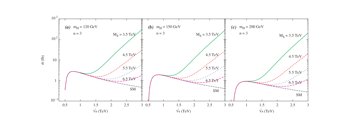
Figure 2: Variation of the cross-section (fb) for $t\bar{t}H$ production with machine energy. The four dashed curves correspond to the ADD predictions for $M_{S}=3.5,4.5$ , $5.5$ and $6.5$ TeV and $n=3$, while the solid line represents the standard model expectations. The three panels correspond to three different values of the Higgs mass.

The cross sections after adding the new amplitudes to the SM are presented in Fig.2 as a function of machine energy, and for different Higgs masses. To be specific, we hold the number of extra dimensions to be $n=3$. In each figure, the solid line represents the standard model predictions and exhibits the expected fall-off with energy. The inclusion of the graviton exchange changes the $\sqrt{s}$-dependence drastically. For relatively large values of $M_{S}$, the fall-off persists upto a certain value of $\sqrt{s}$ and thereafter the cross section increases rapidly. And, as expected, the turnaround point (in $\sqrt{s}$) is a monotonic function of $M_{S}$. Thus we can expect stronger bounds on $M_{S}$ as the machine energy increases. Comparing the three panels in Fig.2, it is very clear that the ADD contribution is not strongly dependent on Higgs mass. At low energies, the difference in the magnitude of cross-sections for these three values of Higgs masses arises mainly from the phase space. At relatively higher value of $\sqrt{s}$, the cross-sections corresponding to $m_{H}=120$ and 200 GeV become nearly identical. Indeed, the relative difference between the cross sections for any two different values of $m_{H}$ tends to be smaller in the ADD case than that within the standard model.

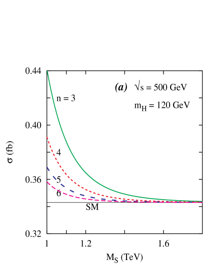
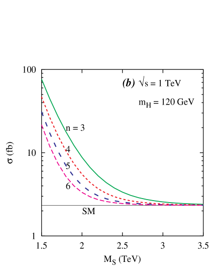
Figure 3: The variation of the cross-section (fb) for $t\bar{t}H$ production with $M_{S}$, for a Higgs mass of 120 GeV. The curves correspond to the ADD predictions for $n=3,4,5$ and $6$ respectively. Also indicated are the standard model expectations. The left and the right panels correspond to $\sqrt{s}=500$ GeV and 1 TeV respectively.

Since the integral in $D(s)$—see eq.(10)—is a relatively slowly increasing function of $(M_{S}/\sqrt{s})$, the amplitudes typically go down as $\sim M_{S}^{-4}$. This is reflected in Fig.3, where we present the total cross-section as a function of $M_{S}$ for theories with different numbers of extra dimensions. For comparison, the SM cross-sections are also given. As with simpler processes, here too the graviton contribution decreases with the increase in the number of extra-dimension as long as the machine energy and $M_{S}$ are held constant.

It is thus obvious that graviton-exchange contributions can significantly alter the predictions for the $e^{+}e^{-}\to t\bar{t}H$ cross-section in such models. However, before one can claim that any such observed deviation has been occasioned by the exchange of virtual gravitons, one needs to ascertain that such deviations cannot be explained by any other possible 4-dimensional new physics effects (4DNP) going beyond the SM. We proceed to do this next.

Note that, within the SM, the process under discussion is controlled by two relatively undetermined couplings, namely the $t\bar{t}H$ and the $ZZH$ ones. Of these, the latter is expected to be measured to a very great accuracy at such a collider [11]. As for the former, the expected accuracy is far less. In fact, the process under consideration, in itself, is perhaps the best channel for this measurement! In view of this ignorance, let us assume that any 4DNP effect may change the $t\bar{t}H$ coupling by at most $10\%$. While this may be an underestimate, we shall see that even a somewhat larger uncertainty would not change our conclusions qualitatively.

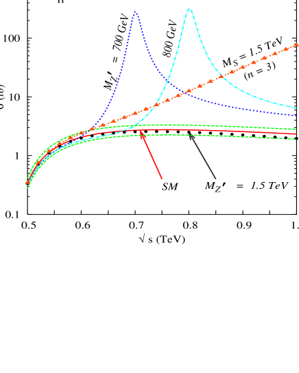
Figure 4: Variation of $\sigma(e^{+}e^{-}\to t\bar{t}H)$ with machine energy ($m_{H}=120\ GeV$). The solid curve represents the SM cross-section while the band around it indicates the variation in it wrought by a $\pm 10\%$ deviation in the SM $t\bar{t}H$ coupling. The monotonically increasing curve corresponds to a ADD model with $n=3$ and $M_{S}=1.5$ TeV. Also shown are three curves corresponding to a 4-dimensional model with a sequential $Z^{\prime}$ for different values of the latter’s mass.

In Fig.4, we display the effect of such a variation in the $t\bar{t}H$ coupling on the cross-section under consideration. The two sidebands around the central (SM) curve represent the cross section expected for an enhancement (reduction) of the $t\bar{t}H$ coupling by $10\%$. As is immediately obvious, the functional dependence of the cross-section on the center-of-mass energy remains virtually the same as in the standard model for modest changes in this coupling. On the other hand, the functional dependence is markedly different for ADD scenarios. Thus, measurements at two different center of mass energies would clearly distinguish between these two classes of models.

As a further example of 4DNP, let us consider an extension of the SM to a model with an extra neutral gauge boson ($Z^{\prime}$). For illustrative purposes, we choose to work with a sequential $Z^{\prime}$, namely one whose couplings to the SM particles are exactly the same as those of the usual $Z$ [12]. In Fig.4, we also demonstrate how the $t\bar{t}H$ production cross section may change in the presence of such a $Z^{\prime}$. For center of mass energies well below $m_{Z^{\prime}}$, the cross section would naturally be quite similar to that within the SM. However, as the energy is raised, the cross section starts to grow rapidly, potentially mimicking the effect within an ADD model. However, if the energy is raised further, the resonance structure characteristic of such a $Z^{\prime}$ would evince itself (as also in other production modes). If the energy were to be raised still further to values much larger than $m_{Z^{\prime}}$, the cross section would fall as dictated by considerations of partial wave unitarity. Thus, once again, such models are easily distinguishable from ADD-like ones.

Now that a method of distinguishing has been delineated, we may try to estimate the sensitivity of the process under consideration. To this end, we display, in Table 1, the $3\sigma$ exclusion limit on $M_{S}$ for different machine energies and number of extra dimensions. In estimating these limits we assume an integrated luminosity of $500~{}{\rm fb}^{-1}$, detection efficiency of $80\%$ and a $2\%$ systematic error. We would, however, like to point out that, in the absence of a detailed simulation, such estimates are necessarily very crude ones. Furthermore, while estimating the SM $tth$ cross-sections we have not considered QCD and EW corrections, which has been computed by several groups [13, 14].

$\sqrt{s}$	$M_{S}$ in GeV
TeV	$n=3$	4	5	6
0.5	920 (880)	855 (825)	810 (785)	780 (750)
1.0	2530 (2470)	2300 (2240)	2140 (2090)	2020 (1970)
3.0	7970 (7680)	7200 (6960)	6680 (6470)	6300 (6100)

Table 1: $3\sigma$ exclusion limits on $M_{S}$ achievable with an integrated luminosity of $500~{}{\rm fb}^{-1}$ for different center-of-mass energies ($\sqrt{s}$). $n$ is the number of extra dimensions and we assume $m_{H}=120$ GeV. The numbers in parentheses refer to the corresponding ($5\sigma$) discovery limits.

That the exclusion limits vary strongly with the available energy is but a consequence of the structure of the theory (in particular, the momentum dependence of the couplings) and could have already been expected from Figs. 2 or  3. What is also remarkable is that the exclusion (discovery) limits on $M_{S}$ are only weakly dependent on the number of extra dimensions.

3 Summary

In this paper we have studied the implications of KK graviton contribution to the process $e^{+}e^{-}\to t\bar{t}H$, which has been studied in the standard model. The spin-2 mode of KK gravitons contribute to this process substantially. It is likely though that the existence of low-energy quantum gravity may be discovered through more direct channels as studied by several groups. Nevertheless, this process will be an independent confirmation for such a discovery. We have shown both $3\sigma$ exclusion limit and $5\sigma$ discovery limit for the string scale $M_{S}$ obtainable at typical linear collider energies assuming the benchmark integrated luminosity of $500~{}{\rm fb}^{-1}$.

References

-
[1]
N. Arkani-Hamed, S. Dimopoulos and G. R. Dvali, Phys. Lett. B429, 263 (1998) ;
Phys. Rev. D 59, 086004 (1999) ;
I. Antoniadis, N. Arkani-Hamed, S. Dimopoulos and G. R. Dvali, Phys. Lett. B436, 257 (1998) . - [2] G. F. Giudice, R. Rattazzi, and J. D. Wells, Nucl. Phys. B544, 3 (1999) .
- [3] T. Han, J. D. Lykken and Ren-Jie Zhang, Phys. Rev. D 59, 105006 (1999) .
-
[4]
For reviews see : T. G. Rizzo, hep-ph/9911229;
Yuri A. Kubyshin, eprint hep-ph/0111027;
J. Hewett and M. Spiropoulu, hep-ph/0205106 and references therein. - [5] N. Akasaka et al. , JLC design study, KEK-REPORT-97-1.
- [6] C. Adolphsen et al. , [International Study Group Collaboration], International study group progress report on linear collider developement, SLAC-R-559 and KEK-REPORT-2000-7 (April, 2000).
- [7] R. D. Heuer et al. , TESLA Technical Design Report: Part III, DESY-2001-011 (hep-ph/0106315.
- [8] R.W. Assmann et al. , [The CLIC Study Team], A 3 TeV linear collider based on CLIC technology, edited by G. Guignard, SLAC-REPRINT-2000-096 and CERN 2000-008.
-
[9]
K.J.Gaemers and G.J.Gounaris, Phys. Lett. B77, 379 (1978) ;
A. Djouadi, J. Kalinowski and P.M. Zerwas, Mod. Phys. Lett. A7, 1765 (1992) and Z. Phys. C54, 255 (1992) . -
[10]
J.F. Gunion, B. Grzadkowski and X.G. He,
Phys. Rev. Lett. 77, 5172 (1996) ;
H. Baer, S. Dawson and L. Reina, Phys. Rev. D 61, 013002 (2000) ;
A. Juste and G. Merino, hep-ph/9910301. - [11] J. Conway, K. Desch, J.F. Gunion, S. Mrenna and D. Zeppenfeld, hep-ph/0203206 and references therein.
- [12] A. Leike, Phys. Rep. 317, 143 (1999) and references therein.
- [13] S. Dittmaier, M. Kramer, Y. Liao, M. Spira and P.M. Zerwas, Phys. Lett. B478, 247 (2000).
- [14] Y. You, W.-G. Ma, H. Chen, R.-Y. Zhang, S.Y. Bin and H.-S. Hou, Phys. Lett. B571, 85 (2003),hep-ph/0306036; G. Belanger, F. Boudjema, J. Fujimoto, T. Ishikawa, T. Kaneko, K. Kato, Y. Shimizu and Y. Yasui, Phys. Lett. B571, 163 (2003), hep-ph/0307029; A. Denner, S. Dittmaier, M. Roth and M.M. Weber, Phys. Lett. B575, 290 (2003). hep-ph/0307193.