Out-of-equilibrium evolution of quantum fields in the hybrid model with quantum back reaction

Abstract

The hybrid model with a scalar ”inflaton” field coupled to a ”Higgs” field with a broken symmetry potential is one of the promising models for inflation and (p)reheating after inflation. We consider the nonequilibrium evolution of the quantum fields of this model with quantum back reaction in the Hartree approximation, in particular the transition of the Higgs field from the metastable ”false vacuum” to the broken symmetry phase. We have performed the renormalization of the equations of motion, of the gap equations and of the energy density, using dimensional regularization. We study the influence of the back reaction on the evolution of the classical fields and of the quantum fluctuations. We observe that back reaction plays an important role over a wide range of parameters. Some implications of our investigation for the preheating stage after cosmic inflation are presented.

I Introduction

The hybrid model has been proposed by Linde Linde:1990gz ; Linde:1991km ; Linde:1994cn as a possible inflationary scenario, several variants of the model have been discussed recently Copeland:1994vg ; Garcia-Bellido:1997wm ; Micha:1999wv ; Buchmuller:2000zm ; Nilles:2001fg ; Asaka:2001ez ; Cormier:2001iw . Here we consider the model in the context of preheating after inflation, and not inflation itself. This period has many interesting aspects and has received a wide attention Garcia-Bellido:1997wm ; Lyth:1998xn ; Garcia-Bellido:1999sv ; Bastero-Gil:1999fz ; Krauss:1999ng ; Felder:2000hj ; Micha:1999wv ; Felder:2001kt ; Copeland:2001qw ; Buchmuller:2000zm ; Nilles:2001fg ; Asaka:2001ez ; Cormier:2001iw ; Garcia-Bellido:2002aj ; Borsanyi:2002tm:Borsanyi:2003ib . For this period it is a reasonable approximation to neglect the coupling to gravity and the expansion of the universe. In hybrid inflation the inflaton transfers at the end of the slow roll period its energy to a Higgs field, whose classical potential changes from a symmetric potential to a double well potential, thereby going through a period of abundant particle production. In the hybrid model two principal mechanisms for particle production are at work: spinodal instability and parametric resonance. Their relative importance depends on the parameters of the particular scenario. The hybrid model may arise naturally in the context of supersymmetry and supergravity Lyth:1998xn ; Bastero-Gil:1999fz ; Micha:1999wv ; Buchmuller:2000zm ; Asaka:2001ez ; it could also display essential features of an electroweak reheating Garcia-Bellido:1999sv ; Garcia-Bellido:2002aj . Another aspect of the type of model investigated here may be that it simulates a first order phase transition, where the change in the effective potential does not arise from a decrease in temperature but is mediated by an effective field. It thereby replaces models Boyanovsky:1997rw ; Bowick:1998kd ; Felder:2000hj ; Felder:2001kt where a rapid decrease of the temperature is simulated by an instantaneous quench.

In this paper we address several new topics:
(i) we include the back reaction of the produced Higgs and inflaton quanta onto the classical Higgs and inflaton fields and onto themselves in the Hartree approximation. This feature limits the exponential growth of fluctuations due to negative squared masses and to parametric resonance, which is unhibited if this back reaction is not included. In previous investigations quantum fluctuations have been included without back reaction Micha:1999wv , with back reaction in the one-loop approximation Cormier:2001iw and in the Hartree approximation with an UV cutoff in a supersymmetric model including axions Bastero-Gil:1999fz . The model investigated there is rather special, it incorporates several scalar degrees of freedom of a non-minimal supersymmetric standard model. So on the one hand it has more scalar fields than the simple hybrid model, on the other hand the couplings are constrained.
(ii) on the formal level we present a consistent renormalization of the gap equations arising in the Hartree approximation, making use of the two-particle point-irreducible (2PPI) formalism Verschelde:1992bs:Coppens:1993zc ; Baacke:2002ee ; Baacke:2003qh . This is a first example of renormalization for coupled channel system out of equilibrium with Hartree-type self-interaction, and goes beyond the one-loop renormalization of Ref. Cormier:2001iw and the unrenormalized Hartree approximation of Ref. Bastero-Gil:1999fz .
(iii) we discuss, as previous authors, the approach to spontaneous symmetry breaking; as in Ref. Garcia-Bellido:2002aj we find that the classical Higgs field approaches the broken symmetry minimum with an exponential behavior. However, we find that for sufficiently high excitations the system does not display a broken symmetry phase at late times; for such excitations the broken symmetry minima are washed out by quantum fluctuations.

We are not able to discuss thermalization, here. Thermalization is not supposed to occur in the Hartree approximation when the fields are homogeneous in space. One of the possibilities in the present context has been discussed in Refs. Asaka:2001ez ; Garcia-Bellido:2002aj : a transition between a quantum description at early times, until the the low energy modes reach high occupation numbers, and appending a classical evolution of this system at late times. For such a classical evolution in a $\Phi^{4}$ model in $1+1$ dimensions thermalization has recently been reported and systematically investigated in Ref. Boyanovsky:2003tc . In a $3+1$ dimensional massless $\Phi^{4}$ model the system is found to evolve towards a turbulent behavior at late times Micha:2002ey . Thermalization and/or “equilibration” has also been discussed within a purely quantum field theoretical description for spatially inhomogeneous fields in the Hartree approximation Salle:2000hd:Salle:2000jb and for spatially homogeneous fields, when going to the next-to-leading order in a $1/N$ expansion within the 2PI formalism (2PI-NLO-1/N) Berges:2001fi ; Aarts:2002dj or to the bare vertex Cooper:2002qd approximations. The issue is not closed at present, and the different approaches have to be studied in conjunction in the future.

The plan of the paper is as follows. We start by briefly reviewing the hybrid model and its application to the preheating stage after cosmic inflation in Sec. II. In Sec. III we present an effective action and the derivation of the equations of motion for the nonequilibrium quantum dynamics in the hybrid model. In Sec. IV we present approximations to the effective action and specify the Hartree approximation by giving the expressions for the fluctuation integrals and the energy contributions. The renormalization is discussed in Sec. V. In Sec. VI we give details of the numerical implementation. The numerical results for different parameter sets are presented and discussed in Sec. VII. We end with conclusions in Sec. VIII. The paper is completed by three appendixes.

II The Hybrid Model

II.1 General form of the potential

We consider the hybrid model as proposed by Linde Linde:1994cn defined by the Lagrange density

$$\mathcal{L}=\frac{1}{2}\partial_{\mu}\Phi\partial^{\mu}\Phi+\frac{1}{2}\partial_{\mu}X\partial^{\mu}X-V(\Phi,X)\ ,$$ (2.1)

with the potential (hybrid potential)

$$V(\Phi,X)=\frac{1}{2}m^{2}\Phi^{2}+\frac{1}{2}g^{2}\Phi^{2}X^{2}+\frac{\lambda}{4}(X^{2}-v^{2})^{2}\ .$$ (2.2)

We will refer to $\Phi$ as the inflaton and to $X$ as the Higgs or the symmetry breaking field. For simplicity the dependence of all fields on the space-time arguments $x=(t,\mathbf{x})$ is suppressed. The discussion will be restricted to a space-time with Minkowski metric. The Higgs field has a double-well potential with a classical vacuum expectation value given by $v$. Both fields $\Phi$ and $X$ are assumed to have non-vanishing classical expectation values (order parameters of the fields), i.e.

$$\left\langle\Phi\right\rangle = \phi\ ,$$ (2.3)

$$\left\langle X\right\rangle = \chi\ .$$ (2.4)

The generic shape of the classical hybrid potential $V(\phi,\chi)$ is shown in Fig. 1. Classically there are the two degenerate minima at the points with $\phi=0$ and $\chi=\pm\lambda v$. They can easily be identified in the contour lines at the base of the plot in Fig. 1. However, if the corrections from quantum fluctuations around the classical solutions are included, the minima of the interacting theory are not equal to the ones in the classical theory.

Figure 1: Generic shape of a hybrid potential $V(\phi,\chi)$ as a function of the classical fields $\phi$ and $\chi$; at the base of this plot the contour lines of the potential are show.

The Higgs field has an effective mass square $m^{2}_{X}(\Phi)=-\lambda v^{2}+g^{2}\Phi^{2}$. Thus the field $X$, i.e. the classical part $\chi$ and its quantum fluctuations, becomes unstable if the absolute value of the inflaton field $\Phi$ is lower than

$$\Phi_{\mathrm{c}}=\frac{v\sqrt{\lambda}}{g}\ .$$ (2.5)

The region with $-\Phi_{\mathrm{c}}<\Phi<\Phi_{\mathrm{c}}$ in the potential is called the spinodal region.

II.2 Energy scales and parameters

If the hybrid model is taken as an effective model for the (p)reheating stage at the end of cosmic inflation, the mass parameters $m^{2}$ and $v^{2}$ and the coupling constants $g$ and $\lambda$ are constrained by the observations of the various cosmic microwave background experiments (see, e.g., Refs. Kinney:2003uw ; Peiris:2003ff ; Barger:2003ym ; Leach:2003us for recent analyzes). In order to fulfill the slow-roll condition the inflaton mass $m$ has to be chosen very small Linde:1994cn

$$m^{2}\ll g^{2}v^{2}\;.$$ (2.6)

This means that the potential in the $\phi$ direction close to $\chi\approx 0$ is very flat. Indeed when treating the period after inflation the inflaton mass $m^{2}$ can be neglected (see, e.g., Copeland:2002ku ); we have chosen $m^{2}=0$ in the numerical simulations throughout. As discussed in Linde:1994cn the couplings $\lambda$ and $g^{2}$ can vary over a wide range, depending on the specific preheating scenario. This is interrelated with the choice of the mass scale $v$ which is chosen to be in the numerical simulations. As we do not couple to gravity its absolute physical value is irrelevant here. Of course this choice enters into the time, momentum and energy scales.

As a concrete phenomenological model it can be embedded at least at two manifestly different energy scales. If one has electroweak preheating Garcia-Bellido:1997wm ; Garcia-Bellido:1999sv ; Garcia-Bellido:2002aj ; Krauss:1999ng ; Copeland:2001qw in mind, the symmetry breaking field mimics the standard Higgs sector of the standard model, while ignoring contributions from the gauge and fermion fields. Of course we would have to generalize $X$ to be a complex doublet in order to represent the SU(2) symmetry breaking Higgs sector. The vacuum expectation value $v$ in this case would be chosen equal to 246GeV. The classical Higgs mass is $m_{\chi}^{2}=\lambda v^{2}$. If the phase transition at the end of inflation takes place at the scale of a Grand Unified Theory (GUT), the symmetry breaking field $X$ could be, e.g., a very heavy sneutrino, i.e. the scalar super-partner of one of the light neutrinos. The reheating in such a scenario would come from the decay of this heavy sneutrino. We will not restrict our study to one of these two scenarios in the following.

III Effective action

III.1 Quantum fluctuations and their non-perturbative resummation

The time evolution of out-of-equilibrium systems in quantum field theory is described within the closed-time-path (CTP) or Schwinger-Keldysh formalism Schwinger:1961qe ; Keldysh:1964ud . Nonequilibrium quantum field theory has seen a tremendous progress, after seminal publications in the 1980’s Cooper:1986wv:Eboli:1988fm , mainly in the last decade Boyanovsky:1993pf:Boyanovsky:1998zg ; Boyanovsky:1997rw ; Boyanovsky:1995me ; Cooper:1994hr:Cooper:1997ii ; Baacke:1997se ; Baacke:1998di ; Baacke:2000fw . The main ingredient, besides the CTP formalism itself, are various approximations based on variational principles. The one-loop, Hartree and and large-$N$ approximations can be based on the two-particle irreducible (2PI) formalism Luttinger:1960ua:deDominicis:1964 ; Cornwall:1974vz . This formalism has also been used beyond these mean field approaches Berges:2000ur ; Berges:2001fi ; Berges:2002cz ; Cooper:2002qd ; Ikeda:2004in . As an alternative approach beyond leading orders we have recently adapted Baacke:2002ee ; Baacke:2003qh the so-called two-particle point irreducible (2PPI) formalism Verschelde:1992bs:Coppens:1993zc ; Verschelde:2000dz to nonequilibrium quantum field theory.

Within the framework outlined above there are several ways for taking into account the quantum fluctuations and their back reaction onto the classical (mean) fields and onto themselves. In any case they should to be treated non-perturbatively, as the amplitudes of the fields can become very large. In practice one resums an infinite number of perturbative Feynman diagrams via a Schwinger-Dyson equation. In this section we will derive all equations of motion, i.e. the classical and quantum equations, from an effective action that incorporates full back reaction of the quantum modes.

Within nonequilibrium quantum field theory the existence of a conserved energy is automatically guaranteed if all equations of motion are derived from the same variational functional, i.e. the effective action. In the context of relativistic quantum field theory Cornwall, Jackiw and Tomboulis (CJT) have derived the 2PI effective action in Ref. Cornwall:1974vz . In addition to a local source term $J(x)$ for a mean field $\phi(x)$ one introduces a bilocal source term $K(x,x^{\prime})$ for the Operator $\left<\Phi(x)\Phi(x^{\prime})\right>=G(x,x^{\prime})+\phi(x)\phi(x^{\prime})$ in the generating functional. The effective action $\Gamma$ follows from a Legendre transformation of the generating functional with variational parameters $\phi(x)$ and $G(x,x^{\prime})$. The leading orders in the 2PI or CJT action exactly reproduce the well know one-loop, large-$N$ and Hartree approximations.

A related effective action is the 2PPI effective action Verschelde:1992bs:Coppens:1993zc ; Verschelde:2000dz . There one has a local source term $K(x,x^{\prime})=K(x)\delta(x-x^{\prime})$ for the composite operator $\left<\Phi^{2}(x)\right>$ thus making all self-energy insertions into the propagator $G(x,x^{\prime})$ local. In the 2PPI effective action formalism the renormalization of the Hartree (and leading order large-$N$) approximation is very transparent, because the non-perturbative counterterms in the effective theory are mapped one-to-one to the standard counterterms of a perturbative expansion of the basic Lagrangian. In addition the 2PPI scheme allows a systematic improvement of the Hartree approximation without all the computational complications from nonlocal self-energies as introduced beyond leading oder in the 2PI scheme.

III.2 The two-particle point-irreducible formalism

At first, a slightly more general Lagrange density for a $N$ component field $\mathbf{\Phi}=(\Phi_{1},\ldots,\Phi_{N})$ is given by

$$\mathcal{L}(x) = \frac{1}{2}\partial_{\mu}\Phi^{i}(x)\partial^{\mu}\Phi^{i}(x)-V(x)\ ,$$ (3.7)

$$V(x) = \frac{1}{2}m_{ij}^{2}\Phi^{i}(x)\Phi^{j}(x)$$ (3.8)

$$+\frac{1}{4!}\lambda_{ijkl}\Phi^{i}(x)\Phi^{j}(x)\Phi^{k}(x)\Phi^{l}(x)\ ,$$

where a summation over $i,j,k,l=1,\ldots,N$ etc. is understood and we have introduced a coupling constant matrix $\lambda_{ijkl}$ and a mass matrix $m_{ij}^{2}$. The fields $\Phi^{i}$ may have classical expectation values, i.e. $\left<\Phi^{i}\right>=\phi^{i}$.

The standard hybrid potential in Eq. (2.2) follows from Eq. (3.8) for the case $N=2$ with the identifications

$$\Phi_{1} = \Phi$$ (3.9)

$$\Phi_{2} = X$$ (3.10)

$$m_{11}^{2} = m^{2}$$ (3.11)

$$m_{22}^{2} = -\lambda v^{2}$$ (3.12)

$$m_{12}^{2} = m_{21}^{2}=0$$ (3.13)

$$\lambda_{2222} = 6\lambda$$ (3.14)

$$\lambda_{\mathrm{Perm}(1122)} = 2g^{2}$$ (3.15)

$$\lambda_{1111} = \lambda_{1112}=\ldots=\lambda_{2221}=0\ .$$ (3.16)

The 2PPI formalism is formulated in terms of the mean fields $\phi^{i}$ and local propagator insertions $\Delta_{ij}$. The local insertions in the propagator are resummed via a Schwinger-Dyson or gap equation. The Green’s function $G$ fulfills the local equation

$$(G^{-1})_{ij}(x,x^{\prime})=i\left(\square\delta_{ij}+{\cal M}^{2}_{ij}(x)\right)\delta^{(D)}(x-x^{\prime})\ ,\$$ (3.17)

where ${\cal M}^{2}_{ij}$ is a variational mass parameter explained below.

For the general potential in Eq. (3.8) the 2PPI effective action can be written as (see e.g. Ref. Verschelde:2000ta ; Verschelde:2000dz )

$$\Gamma[\phi^{i},\Delta^{ij}] = S[\phi^{i}]+\Gamma^{\mathrm{2PPI}}[\phi^{i},{\cal M}^{2}_{ij}]$$ (3.18)

$$+\frac{1}{8}\lambda_{ijkl}\int{d^{D}x}\Delta^{ij}(x)\Delta^{kl}(x)$$

with

$$\Delta^{ij}(x) = -2\frac{\delta\Gamma^{\mathrm{2PPI}}}{\delta{\cal M}^{2}_{ij}(x)}\ .$$ (3.19)

The masses ${\cal M}^{2}_{ij}(x)$ have to fulfill the so called gap equations

$${\cal M}^{2}_{ij}(x) = m_{ij}^{2}+\frac{1}{2}\lambda_{ijkl}\left(\phi^{k}(x)\phi^{l}(x)+\Delta^{kl}(x)\right)\ .\$$ (3.20)

The term $\Gamma^{\mathrm{2PPI}}[\phi^{i},{\cal M}^{2}_{ij}]$ denotes the infinite sum over all 2PPI diagrams. A diagram that does not fall apart if two lines meeting at the same point are cut is called two-particle point-irreducible.

The classical action $S[\phi^{i}]$ is given by

$$S[\phi^{i}] = \int d^{D}x\left[\frac{1}{2}\partial_{\mu}\phi^{i}(x)\partial^{\mu}\phi^{i}(x)-\frac{1}{2}m_{ij}^{2}\phi^{i}(x)\phi^{j}(x)\right.$$ (3.21)

$$\qquad+\left.\frac{1}{4!}\lambda_{ijkl}\phi^{i}(x)\phi^{j}(x)\phi^{k}(x)\phi^{l}(x)\right]\ .$$

The term proportional to an integral over $\Delta^{ij}(x)\Delta^{kl}(x)$ in Eq. (3.18) corrects the double counting of bubble graphs.

With the help of the identifications in Eq. (3.9)–(3.16) the 2PPI effective action for the hybrid potential in Eq. (2.2)reads explicitly

$$\Gamma[\phi,\chi,\Delta_{\phi\phi},\Delta_{\phi\chi},\Delta_{\chi\chi}]$$

$$=S[\phi,\chi]$$

$$+\Gamma^{\mathrm{2PPI}}\left[\phi,\chi,{\cal M}^{2}_{\phi\phi},{\cal M}^{2}_{\phi\chi},{\cal M}^{2}_{\chi\chi}\right]$$

$$+\frac{3\lambda}{4}\int d^{D}x\Delta_{\chi\chi}^{2}(x)$$

$$+\frac{g^{2}}{2}\int d^{D}x\left(\Delta_{\phi\phi}(x)\Delta_{\chi\chi}(x)+2\Delta_{\phi\chi}^{2}(x)\right)\ .$$ (3.22)

The gap equations for the masses ${\cal M}^{2}$ are

$${\cal M}^{2}_{\phi\phi}(x) = m^{2}+g^{2}\left(\chi^{2}(x)+\Delta_{\chi\chi}(x)\right)\ ,$$ (3.23)

$${\cal M}^{2}_{\chi\chi}(x) = -\lambda v^{2}+3\lambda\left(\chi^{2}(x)+\Delta_{\chi\chi}(x)\right)$$ (3.24)

$$\qquad+g^{2}\left(\phi^{2}(x)+\Delta_{\phi\phi}(x)\right)\ ,$$

$${\cal M}^{2}_{\phi\chi}(x) = {\cal M}^{2}_{\chi\phi}(x)=2g^{2}\left(\phi(x)\chi(x)+\Delta_{\phi\chi}(x)\right)\ \ .\$$ (3.25)

The self-energy insertions $\Delta$ are

$$\Delta_{\phi\phi}(x) = -2\frac{\delta\Gamma^{\mathrm{2PPI}}}{\delta{\cal M}^{2}_{\phi\phi}(x)}\ ,$$ (3.26)

$$\Delta_{\chi\chi}(x) = -2\frac{\delta\Gamma^{\mathrm{2PPI}}}{\delta{\cal M}^{2}_{\chi\chi}(x)}\ ,$$ (3.27)

$$\Delta_{\phi\chi}(x) = -2\frac{\delta\Gamma^{\mathrm{2PPI}}}{\delta{\cal M}^{2}_{\phi\chi}(x)}\ .$$ (3.28)

Inverting the gap equations gives

$$\Delta_{\phi\phi}(x) = \frac{1}{g^{2}}\left({\cal M}^{2}_{\chi\chi}(x)+\lambda v^{2}-\frac{3\lambda}{g^{2}}\left({\cal M}^{2}_{\phi\phi}(x)-m^{2}\right)\right)$$ (3.29)

$$-\phi^{2}(x)\ ,$$

$$\Delta_{\chi\chi}(x) = \frac{1}{g^{2}}\left({\cal M}^{2}_{\phi\phi}(x)-m^{2}\right)-\chi^{2}(x)\ ,$$ (3.30)

$$\Delta_{\phi\chi}(x) = \frac{1}{2g^{2}}{\cal M}^{2}_{\phi\chi}(x)-\phi(x)\chi(x)\ .$$ (3.31)

The effective action can therefore be expressed in a form without the $\Delta$’s.

$$\Gamma\left[\phi,\chi,{\cal M}^{2}_{\phi\phi},{\cal M}^{2}_{\chi\chi},{\cal M}^{2}_{\phi\chi}\right]$$ (3.32)

$$= \int d^{D}x\bigg{[}\frac{1}{2}\partial_{\mu}\phi(x)\partial^{\mu}\phi(x)+\frac{1}{2}\partial_{\mu}\chi(x)\partial^{\mu}\chi(x)$$

$$-\frac{1}{2}{\cal M}^{2}_{\phi\phi}(x)\phi^{2}(x)+g^{2}\phi^{2}(x)\chi^{2}(x)$$

$$-\frac{1}{2}{\cal M}^{2}_{\chi\chi}(x)\chi^{2}(x)+\frac{\lambda}{2}\chi^{4}(x)-\frac{\lambda}{4}v^{4}$$

$$-{\cal M}^{2}_{\phi\chi}(x)\phi(x)\chi(x)$$

$$-\frac{3\lambda}{4g^{4}}\left({\cal M}^{2}_{\phi\phi}(x)-m^{2}\right)^{2}$$

$$+\frac{1}{2g^{2}}\left({\cal M}^{2}_{\phi\phi}(x)-m^{2}\right)\left({\cal M}^{2}_{\chi\chi}(x)+\lambda v^{2}\right)$$

$$+\frac{1}{4g^{2}}\left({\cal M}^{2}_{\phi\chi}(x)\right)^{2}\bigg{]}$$

$$+\Gamma^{\mathrm{2PPI}}\left[\phi,\chi,{\cal M}^{2}_{\phi\phi},{\cal M}^{2}_{\phi\chi},{\cal M}^{2}_{\chi\chi}\right]$$

The latter form of the effective action makes it easy to derive a renormalized effective action.

III.3 Equations of motion

The equations of motion for the classical fields $\phi$ and $\chi$ follow from

$$\frac{\delta\Gamma}{\delta\phi(x)}=0\quad\textrm{and}\quad\frac{\delta\Gamma}{\delta\chi(x)}=0\ .$$ (3.33)

If we take only the causal part of all functions by restricting them to the positive time branch of a closed time path (CTP; for the Schwinger-Keldysh closed time path formalism see Ref. Schwinger:1961qe ; Keldysh:1964ud ; Jordan:1986ug ; Calzetta:1988cq ), we get the following classical equations of motion

$$0 = \square\phi+{\cal M}^{2}_{\phi\phi}\phi+{\cal M}^{2}_{\phi\chi}\chi-2g^{2}\chi^{2}\phi$$ (3.35)

$$-\frac{\delta\Gamma^{\mathrm{2PPI}}}{\delta\phi}\ ,$$

$$0 = \square\chi+{\cal M}^{2}_{\chi\chi}\chi+{\cal M}^{2}_{\phi\chi}\phi-2\lambda\chi^{3}-2g^{2}\phi^{2}\chi$$ (3.36)

$$-\frac{\delta\Gamma^{\mathrm{2PPI}}}{\delta\chi}\ .$$

The quantum equations of motion, i.e. the Schwinger-Dyson equations or gap equations, are derived from

$$\frac{\delta\Gamma}{\delta{\cal M}^{2}_{\phi\phi}(x)}=0\,,\,\frac{\delta\Gamma}{\delta{\cal M}^{2}_{\chi\chi}(x)}=0\ \textrm{and}\ \frac{\delta\Gamma}{\delta{\cal M}^{2}_{\phi\chi}(x)}=0\ .$$ (3.37)

They have already been denoted in Eq. (3.23)–(3.25). In general the gap equations form a coupled system of self-consistent nonlinear equations. Due to the self-consistency an infinite number of one-particle irreducible (1PI) diagrams is resummed.

In the following we will assume spatially homogeneous fields. The classical fields obey $\phi=\phi(t)$ and $\chi=\chi(t)$ and the Green’s functions can be expressed via their Fourier components

$$G_{ij}(t,t^{\prime};\mathbf{x},\mathbf{x}^{\prime})=\int\frac{d^{D-1}p}{(2\pi)^{D-1}}e^{i\mathbf{p}\cdot(\mathbf{x}-\mathbf{x}^{\prime})}G_{ij}(t,t^{\prime};\mathbf{p})\ .$$ (3.38)

Since the 2PPI formalism resums local self energy insertions in the Green’s function, $G_{ij}(t,t^{\prime};\mathbf{p})$ can be rewritten in terms of mode functions $f_{i}(t;\mathbf{p})$ and $f_{j}(t^{\prime};\mathbf{p})$. If we do so, we have a Wronskian matrix, that is diagonal. The quantization of the theory at $t=0$ is explained in more detail in Sec. V.1. The Green’s function reads

$$G_{ij}(t,t^{\prime};\mathbf{p}) = \sum_{\alpha=1}^{2}\frac{1}{2\omega_{\alpha}}\bigg{[}f_{i}^{\alpha}(t;p)f_{j}^{*\,\alpha}(t^{\prime};p)\Theta(t-t^{\prime})$$ (3.39)

$$+f_{i}^{\alpha}(t^{\prime};p)f_{j}^{*\,\alpha}(t;p)\Theta(t^{\prime}-t)\bigg{]}\ ,$$

where the mode functions satisfy

$$\ddot{f}_{i}^{\alpha}(t;p)+\left[\mathbf{p}^{2}\delta_{ij}+{\cal M}^{2}_{ij}(t)\right]f_{j}^{\alpha}(t;p)=0\ .$$ (3.40)

The fundamental solutions of this system of coupled differential equations will be labeled with Greek letters $\alpha,\beta,\ldots$. So there are four different complex mode functions.

In Eq. (3.39) we have introduced the quantities $\omega_{\alpha}$ defined by

$$\omega_{\alpha}=\sqrt{\mathbf{p}^{2}+m_{0,\,\alpha}^{2}}\ .$$ (3.41)

They will be explained below, as they depend on the initial conditions via the initial masses $m^{2}_{0,\,\alpha}$.

The explicit form of the equations of motion depends on a given approximation for $\Gamma^{\mathrm{2PPI}}$. In addition one has to renormalize the equations of motion for all approximation schemes beyond the classical, i.e. the tree level.

IV Approximations

The infinite sum of two-particle point-irreducible diagrams in $\Gamma^{\mathrm{2PPI}}$ can be truncated in several ways. We will discuss a loop expansion here. The loop expansion can be formulated as

$$\Gamma^{\mathrm{2PPI}}=\sum_{\ell=1}^{\infty}\Gamma^{(\ell)}=\Gamma^{(1)}+\Gamma^{(2)}+\ldots\ ,$$ (4.1)

where the index $\ell=1,2,\ldots$ corresponds to the number of loops in a 2PPI diagram. The dots in the last equation indicates all contributions beyond the two-loop order. The fluctuation integrals $\Delta_{ij}$ are expanded analogous as

$$\Delta_{ij}(t)=\Delta_{ij}^{(1)}(t)+\Delta_{ij}^{(2)}(t)+\ldots.$$ (4.2)

The one-loop order in the 2PPI loop expansion is equivalent to the Hartree approximation, as already stated above.

Zero-loop – classical approximation.

To zero-loop order one discards the term $\Gamma^{\mathrm{2PPI}}$ completely, which leads to $\Delta_{ij}=0$ and $\frac{\delta\Gamma^{\mathrm{2PPI}}}{\delta\phi}=\frac{\delta\Gamma^{\mathrm{2PPI}}}{\delta\chi}=0$.

The zero-loop contribution to the energy denotes

$$E^{(0)}(t) = \frac{1}{2}\dot{\phi}^{2}(t)+\frac{1}{2}{\cal M}^{2}_{\phi\phi}(t)\phi^{2}(t)-g^{2}\phi^{2}(t)\chi^{2}(t)$$

$$+\frac{1}{2}\dot{\chi}^{2}(t)+\frac{1}{2}{\cal M}^{2}_{\chi\chi}(t)\chi^{2}(t)-\frac{\lambda}{2}\chi^{4}(t)+\frac{\lambda}{4}v^{4}$$

$$+{\cal M}^{2}_{\phi\chi}(t)\phi(t)\chi(t)-\frac{1}{4g^{2}}\left({\cal M}^{2}_{\phi\chi}(t)\right)^{2}$$

$$+\frac{3\lambda}{4g^{4}}\left({\cal M}^{2}_{\phi\phi}(t)-m^{2}\right)^{2}$$

$$-\frac{1}{2g^{2}}\left({\cal M}^{2}_{\phi\phi}(t)-m^{2}\right)\left({\cal M}^{2}_{\chi\chi}(t)+\lambda v^{2}\right)\ .$$

One-loop – Hartree approximation.

The one-loop approximation is identical to what we will call Hartree approximation. The sum of all two-particle point-irreducible diagrams is truncated at $\Gamma^{\mathrm{2PPI}}\approx\Gamma^{(1)}$ with (see the diagram in Fig. 2)

$$\Gamma^{(1)}[{\cal M}^{2}_{\phi\phi},{\cal M}^{2}_{\chi\chi},{\cal M}^{2}_{\phi\chi}]=\frac{i}{2}\mathrm{Tr}\ln\left[\mathcal{G}^{-1}\right]\ .$$ (4.4)

We have introduced

$$\mathcal{G}=\begin{pmatrix}G_{\phi\phi}&G_{\phi\chi}\cr G_{\chi\phi}&G_{\chi\chi}\end{pmatrix}\ .$$ (4.5)

Figure 2: One-loop bubble diagram representing the Hartree approximation. The line denotes a propagator $\mathcal{G}$ as given by Eq. (4.5)

The functional derivative of $\Gamma^{(1)}$ with respect to ${\cal M}^{2}_{ij}$ gives the tadpole insertions

$$\Delta_{ij}^{(1)}(t) = \frac{1}{2}\int\frac{d^{D-1}p}{(2\pi)^{D-1}}\bigg{[}G_{ij}(t,t;\mathbf{p})+G_{ji}(t,t;\mathbf{p})\bigg{]}$$

$$= \sum_{\alpha=1}^{2}\int\frac{d^{D-1}p}{(2\pi)^{D-1}}\frac{1}{2\omega_{\alpha}}\mathrm{Re}\left[f_{i}^{\alpha}(t;p)f_{j}^{\alpha\,*}(t;p)\right]\ .$$

There a three different insertions, $\Delta_{\phi\phi}^{(1)}$, $\Delta_{\chi\chi}^{(1)}$ and $\Delta_{\phi\chi}^{(1)}=\Delta_{\chi\phi}^{(1)}$. The gap equations (3.23)–(3.25) resum one-loop bubble graphs, because the Green’s functions $G_{ij}$ depend on the variational mass parameters ${\cal M}^{2}_{ij}$. At one-loop order we have $\frac{\delta\Gamma^{\mathrm{2PPI}}}{\delta\phi}=\frac{\delta\Gamma^{\mathrm{2PPI}}}{\delta\chi}=0$.

The contribution of the bubble graphs to the energy is defined by the relation

$$\frac{dE^{(1)}(t)}{dt} = -\frac{\delta\Gamma^{(1)}[{\cal M}^{2}_{\phi\phi},{\cal M}^{2}_{\chi\chi},{\cal M}^{2}_{\phi\chi}]}{\delta{\cal M}^{2}_{ij}(t)}\frac{d{\cal M}^{2}_{ij}(t)}{dt}$$

$$= \frac{1}{2}\int\frac{d^{D-1}p}{(2\pi)^{D-1}}G_{ij}(t,t;\mathbf{p})\frac{d{\cal M}^{2}_{ij}(t)}{dt}$$

This equation can be integrated explicitly if one uses the equations of motion for the mode functions $f_{i}^{\alpha}(t;p)$, yielding

$$E^{(1)}(t) = \frac{1}{2}\int\frac{d^{D-1}p}{(2\pi)^{D-1}}\sum_{\alpha}\frac{1}{2\omega_{\alpha}}$$ (4.9)

$$\times\Bigg{\{}\mathrm{Re}\left[\dot{f}_{\phi}^{\alpha}(t;p)\dot{f}_{\phi}^{\alpha\,*}(t;p)\right]$$

$$\qquad+\mathrm{Re}\left[\dot{f}_{\chi}^{\alpha}(t;p)\dot{f}_{\chi}^{\alpha\,*}(t;p)\right]$$

$$\qquad+\left(\mathbf{p}^{2}+{\cal M}^{2}_{\phi\phi}(t)\right)\mathrm{Re}\left[f_{\phi}^{\alpha}(t;p)f_{\phi}^{\alpha\,*}(t;p)\right]$$

$$\qquad+\left(\mathbf{p}^{2}+{\cal M}^{2}_{\chi\chi}(t)\right)\mathrm{Re}\left[f_{\chi}^{\alpha}(t;p)f_{\chi}^{\alpha\,*}(t;p)\right]$$

$$\qquad+2{\cal M}^{2}_{\phi\chi}(t)\mathrm{Re}\left[f_{\phi}^{\alpha}(t;p)f_{\chi}^{\alpha\,*}(t;p)\right]\Bigg{\}}\ .$$

The momentum integrations in the quantities $\Delta^{(1)}$ and $E^{(1)}$ are divergent and thus have to be renormalized properly. We will discuss this issue in the next section.

Two-loop – sunset diagrams

The only two-loop diagram appearing is the sunset diagram displayed in Fig. 3. This sunset graph leads to time integrations over the past of classical and quantum fields (“memory integrations”) and introduces scattering of the quanta (see Ref. Baacke:2002ee ; Baacke:2003qh for two-loop simulations of $\Phi^{4}$ theory in 1+1 dimensions). While it would be interesting to study how this next-to-leading order diagram affects the dynamics studied here, this is beyond the scope of this work.

Figure 3: Two-loop sunset diagram; the solid lines denote the propagator $\mathcal{G}$, the dashed lines the classical fields $\varphi=(\phi,\chi)$.

V Renormalization

V.1 Initial conditions

The choice of initial conditions for the quantum system has to be discussed together with its renormalization. We will take a Gaussian initial density matrix with non-vanishing initial values $\phi(t=0)$ and $\chi(t=0)$ for the classical field amplitudes. For the renormalization of the equations of motion we need a properly quantized system at the initial time. In order to satisfy the usual canonical commutation relations for the creation and annihilation operators of the quantum fields, we choose a Fock space basis at $t=0$. The basic quanta are defined by diagonalizing the mass matrix at $t=0$ and by choosing canonical initial conditions (see below) for the mode functions (see e.g. Baacke:1997se ; Baacke:2000fw ; Cormier:2001iw ; Nilles:2001fg )

We define the initial masses $m_{0,\alpha}$ as the eigenvalues of the initial mass matrix ${\cal M}_{ij}(0)$, i.e., by the equation

$$m_{0,\,\alpha}^{2}f_{i}^{\alpha}(0;p)-{\cal M}^{2}_{ij}(0)f_{j}^{\alpha}(0;p) = 0\ .$$ (5.1)

The eigenvalues are given by

$$m_{0,\,\alpha}^{2} = \frac{1}{2}\bigg{[}{\cal M}^{2}_{\phi\phi}(0)+{\cal M}^{2}_{\chi\chi}(0)$$ (5.2)

$$\pm\sqrt{\left({\cal M}^{2}_{\phi\phi}(0)-{\cal M}^{2}_{\chi\chi}(0)\right)^{2}+4{\cal M}^{4}_{\phi\chi}(0)}\bigg{]}\ .$$

We denote the corresponding eigenvectors by $O_{i\alpha}$, where the index $\alpha$ refers to the eigenvalue, and the latin indices to the components. The canonical initial conditions at $t=0$ for the mode functions are

$$f_{i}^{\alpha}(0;p) = O_{i\alpha}$$ (5.3)

$$\dot{f}_{i}^{\alpha}(0;p) = -i\omega_{\alpha}O_{i\alpha}=-i\omega_{\alpha}f_{i}^{\alpha}(0;p)\ .$$ (5.4)

The Wronskian matrix of these mode functions is then given by

$$W(f^{\alpha}_{i},f^{\beta}_{i}) = [f_{i}^{\alpha,\,*}(0;p)\dot{f}_{i}^{\beta}(0;p)$$ (5.5)

$$-\dot{f}_{i}^{\alpha,\,*}(0;p)f_{i}^{\beta}(0;p)]$$

$$= -i[(\omega_{\alpha}+\omega_{\beta})O_{i\alpha}O_{i\beta}]\ .$$ (5.6)

As the eigenvectors are orthogonal this matrix is diagonal. Choosing the normalization

$$O_{i\alpha}O_{i\beta}=\delta_{\alpha\beta}$$ (5.7)

the Wronskian matrix becomes

$$W(f^{\alpha}_{i},f^{\beta}_{i})_{\alpha,\beta=1,2} = -2i\begin{pmatrix}\omega_{1}&0\cr 0&\omega_{2}\end{pmatrix}\;.$$ (5.8)

If ${\cal M}^{2}_{\chi\chi}(0)>{\cal M}^{2}_{\phi\phi}(0)$ we can fix the matrix $O$ as

$$O = \begin{pmatrix}\cos\vartheta&\sin\vartheta\cr-\sin\vartheta&\cos\vartheta\end{pmatrix}\ ,$$ (5.9)

$$\tan\vartheta = \frac{1}{2{\cal M}^{2}_{\phi\chi}(0)}\bigg{\{}{\cal M}^{2}_{\chi\chi}(0)-{\cal M}^{2}_{\phi\phi}(0)$$ (5.10)

$$\quad+\sqrt{\left[{\cal M}^{2}_{\chi\chi}(0)-{\cal M}^{2}_{\phi\phi}(0)\right]^{2}+4{\cal M}^{4}_{\phi\chi}(0)}\bigg{\}}$$

For the opposite case ${\cal M}^{2}_{\chi\chi}(0)<{\cal M}^{2}_{\phi\phi}(0)$ one should interchange $m_{0,\,1}^{2}$ with $m_{0,\,2}^{2}$ and switch $\vartheta\to-\vartheta$.

V.2 Isolation of the divergent contributions

The propagator insertions $\Delta_{ij}^{(1)}$ in Eq. (IV) are divergent. First we have to isolate the divergent contributions from the finite parts. Then the renormalization can be performed within a suitable regularization scheme.

A strategy for the isolation of the divergences via the perturbative expansion of the mode functions in terms of partial integrations has been described in Refs. Baacke:1997se ; Baacke:1997kj . We have summarized what we need in Appendix B.

In dimensional regularization with the abbreviation $L_{\epsilon}=\frac{2}{\epsilon}-\gamma+\ln 4\pi$ we have, using Eq. (B63) from Appendix B and Eq. (A48) and (A51) from Appendix A

$$\Delta_{ij}^{(1)}(t) = \frac{1}{2}\int\frac{d^{D-1}p}{(2\pi)^{D-1}}\bigg{[}G_{ij}(t,t;\mathbf{p})+G_{ji}(t,t;\mathbf{p})\bigg{]}$$ (5.11)

$$= -\sum_{\alpha}\bigg{[}\frac{m_{0,\,\alpha}^{2}}{16\pi^{2}}\bigg{(}L_{\epsilon}-\ln\frac{m_{0,\,\alpha}^{2}}{\mu^{2}}+1\bigg{)}O_{i\alpha}O_{j\alpha}$$

$$\quad+\frac{1}{16\pi^{2}}\bigg{(}L_{\epsilon}-\ln\frac{m_{0,\,\alpha}^{2}}{\mu^{2}}+1\bigg{)}$$

$$\quad+\frac{1}{16\pi^{2}}\sum_{\beta}\bigg{(}\frac{m_{0,\,\beta}^{2}}{m_{0,\,\alpha}^{2}-m_{0,\,\beta}^{2}}\ln\frac{m_{0,\,\beta}^{2}}{m_{0,\,\alpha}^{2}}\bigg{)}$$

$$\quad\,\times\,O_{i\alpha}O_{j\beta}O_{l\beta}O_{k\alpha}\mathcal{V}_{kl}(t)\bigg{]}\quad+\ldots$$

$$= -\frac{1}{16\pi^{2}}\left[L_{\epsilon}+1\right]{\cal M}^{2}_{ij}(t)$$

$$+\sum_{\alpha}\frac{m_{0,\,\alpha}^{2}}{16\pi^{2}}O_{i\alpha}O_{j\alpha}\ln\frac{m_{0,\,\alpha}^{2}}{\mu^{2}}$$

$$+\frac{1}{16\pi^{2}}\sum_{\alpha,\beta}O_{i\alpha}O_{j\beta}O_{l\beta}O_{k\alpha}\mathcal{V}_{kl}(t)$$

$$\times\bigg{(}\ln\frac{m_{0,\,\alpha}^{2}}{\mu^{2}}-\frac{m_{0,\,\beta}^{2}}{m_{0,\,\alpha}^{2}-m_{0,\,\beta}^{2}}\ln\frac{m_{0,\,\beta}^{2}}{m_{0,\,\alpha}^{2}}\bigg{)}\quad$$

$$+\ldots\ ,$$

where $\sum_{\alpha}O_{i\alpha}O_{j\alpha}m_{0,\,\alpha}^{2}={\cal M}^{2}_{ij}(0)$ has been used. The potential $\mathcal{V}_{ij}(t)$ is defined as

$$\mathcal{V}_{ij}(t) = {\cal M}^{2}_{ij}(t)-{\cal M}^{2}_{ij}(0)\ .$$ (5.12)

We can define the finite part of $\Delta_{ij}^{(1)}$ by a subtraction as [see Eq. (B63)]

$$\Delta_{ij,\,\mathrm{fin}}^{(1)}(t) = \int\frac{d^{D-1}p}{(2\pi)^{D-1}}\sum_{\alpha,\beta}\frac{1}{2\omega_{\alpha}}$$

$$\times\bigg{\{}\mathrm{Re}\left[f_{i}^{\alpha}(t;p)f_{j}^{\alpha,\,*}(t;p)\right]\delta_{\alpha\beta}$$

$$\quad-O_{i\alpha}O_{j\alpha}\delta_{\alpha\beta}$$

$$\quad+\frac{1}{\omega_{\beta}(\omega_{\alpha}+\omega_{\beta})}O_{i\alpha}O_{j\beta}O_{l\beta}O_{k\alpha}\mathcal{V}_{kl}(t)\bigg{\}}\ .$$

The momentum integrations in this expression are convergent, because the subtracted terms cancel exactly the divergent parts. There are different finite contributions from the divergent part of $\Delta_{ij}^{(1)}$ (see. Eq. (5.11)). We find it useful to define the following quantities

$$C^{0}_{ij} = \frac{1}{16\pi^{2}}\sum_{\alpha}O_{i\alpha}O_{j\alpha}m_{0,\,\alpha}^{2}\ln\frac{m_{0,\,\alpha}^{2}}{\mu^{2}}$$ (5.14)

$$C^{k\ell}_{ij} = \frac{1}{16\pi^{2}}\sum_{\alpha,\beta}O_{i\alpha}O_{j\beta}O_{k\alpha}O_{\ell\beta}$$ (5.15)

$$\times\bigg{(}\ln\frac{m_{0,\,\alpha}^{2}}{\mu^{2}}-\frac{m_{0,\,\beta}^{2}}{m_{0,\,\alpha}^{2}-m_{0,\,\beta}^{2}}\ln\frac{m_{0,\,\beta}^{2}}{m_{0,\,\alpha}^{2}}\bigg{)}$$

and

$$C^{1}_{ij}:=C^{11}_{ij}\,,\quad C^{2}_{ij}:=C^{22}_{ij}\,,\quad C^{3}_{ij}:=C^{12}_{ij}+C^{21}_{ji}\ .$$ (5.16)

Thus the full 2PPI insertion $\Delta_{ij}^{(1)}$ takes a very simple form given by

$$\Delta_{ij}^{(1)}(t) = \Delta_{ij,\mathrm{fin}}^{(1)}(t)-\frac{1}{16\pi^{2}}\left[L_{\epsilon}+1\right]{\cal M}^{2}_{ij}(t)$$ (5.17)

$$+C^{0}_{ij}+C^{1}_{ij}\left({\cal M}^{2}_{\phi\phi}(t)-{\cal M}^{2}_{\phi\phi}(0)\right)$$

$$+C^{2}_{ij}\left({\cal M}^{2}_{\chi\chi}(t)-{\cal M}^{2}_{\chi\chi}(0)\right)$$

$$+C^{3}_{ij}\left({\cal M}^{2}_{\phi\chi}(t)-{\cal M}^{2}_{\phi\chi}(0)\right)\ .$$

As one can see the divergent part of $\Delta_{ij}^{(1)}$ is directly proportional to ${\cal M}^{2}_{ij}$, i.e. with a uniform factor for all combinations of $i$ and $j$. In particular it is independent of the masses $m_{0,\,\alpha}^{2}$ and the matrix $O_{ij}$ and thereby of the initial conditions. On the other hand the different finite parts depend on the initial conditions via the constants $C_{ij}^{n}$ and involve all components of the effective mass matrix ${\cal M}^{2}_{ij}$.

V.3 Suitable effective counterterms for the gap equations

The divergent part in Eq. (5.17) will be removed by effective mass counter terms. We explain in Appendix C how the effective mass counterterms we are using here are related to standard mass and coupling constant counterterms in a standard counterterm Lagrangian. More precisely the 2PPI formalism establishes a one-to-one mapping between both counterterm approaches.

In order to have a $\delta{\cal M}^{2}$ counterterm in the gap equations, we add to the effective action in Eq. (3.32) a counterterm of the general form

$$\delta{\cal M}^{4} = \delta\xi_{\phi\phi}\left({\cal M}^{2}_{\phi\phi}\right)^{2}+\delta\xi_{\chi\chi}\left({\cal M}^{2}_{\chi\chi}\right)^{2}$$ (5.18)

$$+2\,\delta\xi_{\phi\chi}\left({\cal M}^{2}_{\phi\chi}\right)^{2}$$

With the introduced effective mass counterterms the renormalized gap equations take the form

$${\cal M}^{2}_{\mathrm{R},\,\phi\phi}(t) = m^{2}+g^{2}\left(\chi^{2}(t)+\Delta_{\chi\chi}(t)\right)$$ (5.19)

$$-4g^{2}\,\delta\xi_{\chi\chi}{\cal M}^{2}_{\mathrm{R},\chi\chi}(t)$$

$${\cal M}^{2}_{\mathrm{R},\,\chi\chi}(t) = -\lambda v^{2}+g^{2}\left(\phi^{2}(t)+\Delta_{\phi\phi}(t)\right)$$

$$+3\lambda\left(\chi^{2}(t)+\Delta_{\chi\chi}(t)\right)$$

$$-4g^{2}\,\delta\xi_{\phi\phi}{\cal M}^{2}_{\mathrm{R},\,\phi\phi}(t)-12\lambda\,\delta\xi_{\chi\chi}{\cal M}^{2}_{\mathrm{R},\,\chi\chi}(t)$$

$${\cal M}^{2}_{\mathrm{R},\,\phi\chi}(t) = 2g^{2}\left(\phi(t)\chi(t)+\Delta_{\phi\chi}(t)\right)$$ (5.21)

$$-8g^{2}\,\delta\xi_{\phi\chi}{\cal M}^{2}_{\mathrm{R},\,\phi\chi}(t)\ .$$

By inserting $\Delta_{ij}(t)$ from Eq. (5.17) one can see that the gap equations become finite if we choose

$$\delta\xi_{\phi\phi}=\delta\xi_{\chi\chi}=\delta\xi_{\phi\chi} = -\frac{1}{64\pi^{2}}\left[L_{\epsilon}+1\right]$$

$$= -\frac{1}{64\pi^{2}}\left(\frac{2}{\epsilon}-\gamma+1+\ln 4\pi\right)\ .$$

This choice of $\delta\xi$ corresponds to a $\overline{\mathrm{MS}}$ prescription. In particular, the renormalization scheme is mass independent. Thus the system of renormalized gap equations is finally given by

$${\cal M}^{2}_{\mathrm{R},\,\phi\phi}(t) = m^{2}+g^{2}\left(\chi^{2}(t)+\Delta_{\chi\chi,\mathrm{fin}}(t)\right)$$

$$+g^{2}C^{0}_{\chi\chi}$$

$$+g^{2}C^{1}_{\chi\chi}\left({\cal M}^{2}_{\mathrm{R},\,\phi\phi}(t)-{\cal M}^{2}_{\mathrm{R},\,\phi\phi}(0)\right)$$

$$+g^{2}C^{2}_{\chi\chi}\left({\cal M}^{2}_{\mathrm{R},\,\chi\chi}(t)-{\cal M}^{2}_{\mathrm{R},\,\chi\chi}(0)\right)$$

$$+g^{2}C^{3}_{\chi\chi}\left({\cal M}^{2}_{\mathrm{R},\,\phi\chi}(t)-{\cal M}^{2}_{\mathrm{R},\,\phi\chi}(0)\right)\ ,$$

$${\cal M}^{2}_{\mathrm{R},\,\chi\chi}(t) = -\lambda v^{2}+g^{2}\left(\phi^{2}(t)+\Delta_{\phi\phi,\mathrm{fin}}(t)\right)$$

$$+g^{2}C^{0}_{\phi\phi}$$

$$+g^{2}C^{1}_{\phi\phi}\left({\cal M}^{2}_{\mathrm{R},\,\phi\phi}(t)-{\cal M}^{2}_{\mathrm{R},\,\phi\phi}(0)\right)$$

$$+g^{2}C^{2}_{\phi\phi}\left({\cal M}^{2}_{\mathrm{R},\,\chi\chi}(t)-{\cal M}^{2}_{\mathrm{R},\,\chi\chi}(0)\right)$$

$$+g^{2}C^{3}_{\phi\phi}\left({\cal M}^{2}_{\mathrm{R},\,\phi\chi}(t)-{\cal M}^{2}_{\mathrm{R},\,\phi\chi}(0)\right)$$

$$+3\lambda\left(\chi^{2}(t)+\Delta_{\chi\chi,\mathrm{fin}}(t)\right)+3\lambda C^{0}_{\chi\chi}$$

$$+3\lambda C^{1}_{\chi\chi}\left({\cal M}^{2}_{\mathrm{R},\,\phi\phi}(t)-{\cal M}^{2}_{\mathrm{R},\,\phi\phi}(0)\right)$$

$$+3\lambda C^{2}_{\chi\chi}\left({\cal M}^{2}_{\mathrm{R},\,\chi\chi}(t)-{\cal M}^{2}_{\mathrm{R},\,\chi\chi}(0)\right)$$

$$+3\lambda C^{3}_{\chi\chi}\left({\cal M}^{2}_{\mathrm{R},\,\phi\chi}(t)-{\cal M}^{2}_{\mathrm{R},\,\phi\chi}(0)\right)\ ,$$

$${\cal M}^{2}_{\mathrm{R},\,\phi\chi}(t) = 2g^{2}\left(\phi(t)\chi(t)+\Delta_{\phi\chi,\mathrm{fin}}(t)\right)$$

$$+2g^{2}C^{0}_{\phi\chi}$$

$$+2g^{2}C^{1}_{\phi\chi}\left({\cal M}^{2}_{\mathrm{R},\,\phi\phi}(t)-{\cal M}^{2}_{\mathrm{R},\,\phi\phi}(0)\right)$$

$$+2g^{2}C^{2}_{\phi\chi}\left({\cal M}^{2}_{\mathrm{R},\,\chi\chi}(t)-{\cal M}^{2}_{\mathrm{R},\,\chi\chi}(0)\right)$$

$$+2g^{2}C^{3}_{\phi\chi}\left({\cal M}^{2}_{\mathrm{R},\,\phi\chi}(t)-{\cal M}^{2}_{\mathrm{R},\,\phi\chi}(0)\right)\ .$$

This system of linear equations is similar to the one appearing in the $O(N)$-model in the Hartree approximation Baacke:2001zt . It has to be solved at each time. However, the coefficient matrix can be diagonalized with a time-independent rotation matrix, because it is time independent itself. Such a rotation matrix is analogous to the factor $\mathcal{C}=(1+\frac{\lambda}{16\pi^{2}}\ln\frac{m^{2}}{m_{0}^{2}})^{-1}$ in the renormalization of the $O(N)$-model in the large-$N$ approximation Baacke:2000fw .

V.4 Renormalized energy

Within the Hartree approximation the contributions to the energy introduce logarithmic, quadratic and quartic divergences. The divergences have to be compensated by the already fixed counterterms of the last section.

If the effective masses are identified by the renormalized effective masses of the previous section, then the zero-loop contribution to the energy [see Eq. (IV)] is automatically renormalized.

In the following we use the rotated potential $\widetilde{\mathcal{V}}$ defined by

$$\widetilde{\mathcal{V}}_{\alpha\beta}(t) = O_{k\alpha}\mathcal{V}_{kl}(t)O_{l\beta}$$ (5.27)

$$= O_{1\alpha}O_{1\beta}\mathcal{V}_{\phi\phi}(t)+O_{2\alpha}O_{2\beta}\mathcal{V}_{\chi\chi}(t)$$

$$+(O_{1\alpha}O_{2\beta}+O_{2\alpha}O_{1\beta})\mathcal{V}_{\phi\chi}(t)\$$

According to the expansion of the mode functions in Appendix B the divergent part of the one-loop contribution from the bubble graphs to the quantum energy is given by [see Eq. (B74)]

$$E^{(1),\,\mathrm{div}}(t) = \frac{1}{2}\int\frac{d^{D-1}p}{(2\pi)^{D-1}}\sum_{\alpha}\frac{1}{2\omega_{\alpha}}\bigg{[}2\omega_{\alpha}^{2}+\widetilde{\mathcal{V}}_{\alpha\alpha}(t)$$ (5.28)

$$-\sum_{\beta}\frac{1}{2\omega_{\beta}(\omega_{\alpha}+\omega_{\beta})}\widetilde{\mathcal{V}}_{\alpha\beta}(t)\widetilde{\mathcal{V}}_{\alpha\beta}(t)\bigg{]}\ .\quad\qquad$$

The first term is quartic divergent. Its renormalization corresponds to a renormalization of the cosmological constant $\Lambda$; it is therefore somewhat arbitrary and can be omitted.

If the divergent parts are evaluated in dimensional regularization [using Eq. (A48), (A51) and (A55) in Appendix A] the full one-loop contribution in Eq. (4.9) denotes

$$E^{(1)}(t) = E^{(1)}_{\mathrm{fin}}(t)+\sum_{\alpha}\frac{m_{0,\,\alpha}^{4}}{64\pi^{2}}\left[L_{\epsilon}-\ln\frac{m_{0,\,\alpha}^{2}}{\mu^{2}}+\frac{3}{2}\right]$$ (5.29)

$$-\sum_{\alpha}\frac{m_{0,\,\alpha}^{2}}{32\pi^{2}}\widetilde{\mathcal{V}}_{\alpha\alpha}(t)\left[L_{\epsilon}-\ln\frac{m_{0,\,\alpha}^{2}}{\mu^{2}}+1\right]$$

$$-\sum_{\alpha,\,\beta}\frac{1}{64\pi^{2}}\widetilde{\mathcal{V}}_{\alpha\beta}(t)\widetilde{\mathcal{V}}_{\alpha\beta}(t)$$

$$\times\bigg{[}L_{\epsilon}-\ln\frac{m_{0,\,\alpha}^{2}}{\mu^{2}}+1$$

$$\qquad+\frac{m_{0,\,\beta}^{2}}{m_{0,\,\alpha}^{2}-m_{0,\,\beta}^{2}}\ln\frac{m_{0,\,\beta}^{2}}{m_{0,\,\alpha}^{2}}\bigg{]}\ ,$$

where the finite part has been defined as

$$E^{(1)}_{\mathrm{fin}}(t) = \frac{1}{2}\int\frac{d^{D-1}p}{(2\pi)^{D-1}}\sum_{\alpha}\frac{1}{2\omega_{\alpha}}$$ (5.30)

$$\,\times\Bigg{\{}\mathrm{Re}\left[\dot{f}_{\phi}^{\alpha}(t;p)\dot{f}_{\phi}^{\alpha\,*}(t;p)\right]$$

$$\quad+\mathrm{Re}\left[\dot{f}_{\chi}^{\alpha}(t;p)\dot{f}_{\chi}^{\alpha\,*}(t;p)\right]$$

$$\quad+\left(\mathbf{p}^{2}+{\cal M}^{2}_{\phi\phi}(t)\right)\mathrm{Re}\left[f_{\phi}^{\alpha}(t;p)f_{\phi}^{\alpha\,*}(t;p)\right]$$

$$\quad+\left(\mathbf{p}^{2}+{\cal M}^{2}_{\chi\chi}(t)\right)\mathrm{Re}\left[f_{\chi}^{\alpha}(t;p)f_{\chi}^{\alpha\,*}(t;p)\right]$$

$$\quad+2{\cal M}^{2}_{\phi\chi}(t)\mathrm{Re}\left[f_{\phi}^{\alpha}(t;p)f_{\chi}^{\alpha\,*}(t;p)\right]$$

$$\quad-2\omega_{\alpha}^{2}-\widetilde{\mathcal{V}}_{\alpha\alpha}(t)$$

$$\quad+\sum_{\beta}\frac{1}{2\omega_{\beta}(\omega_{\alpha}+\omega_{\beta})}\widetilde{\mathcal{V}}_{\alpha\beta}(t)\widetilde{\mathcal{V}}_{\alpha\beta}(t)\Bigg{\}}\ .$$

From the definition of $m_{0,\,\alpha}^{2}$ and $\widetilde{\mathcal{V}}_{\alpha\beta}(t)$ one can prove the identity

$$\sum_{\alpha}\bigg{[}m_{0,\,\alpha}^{4}-2m_{0,\,\alpha}^{2}\widetilde{\mathcal{V}}_{\alpha\alpha}(t)-\sum_{\beta}\widetilde{\mathcal{V}}_{\alpha\beta}(t)\widetilde{\mathcal{V}}_{\alpha\beta}(t)\bigg{]}$$

$$=-{\cal M}^{2}_{ij}(t){\cal M}^{2}_{ij}(t)\ ,$$ (5.31)

so that the divergent part becomes very simple. The full quantum energy $E^{(1)}$ is then given by

$$E^{(1)}(t) = E^{(1)}_{\mathrm{fin}}(t)-\frac{1}{64\pi^{2}}\left[L_{\epsilon}+1\right]{\cal M}^{2}_{ij}(t){\cal M}^{2}_{ij}(t)$$ (5.32)

$$+\sum_{\alpha}\frac{m_{0,\,\alpha}^{4}}{64\pi^{2}}\left[-\ln\frac{m_{0,\,\alpha}^{2}}{\mu^{2}}+\frac{1}{2}\right]$$

$$+\sum_{\alpha}\frac{m_{0,\,\alpha}^{2}}{32\pi^{2}}\widetilde{\mathcal{V}}_{\alpha\alpha}(t)\ln\frac{m_{0,\,\alpha}^{2}}{\mu^{2}}$$

$$+\sum_{\alpha,\beta}\frac{1}{64\pi^{2}}\widetilde{\mathcal{V}}_{\alpha\beta}(t)\widetilde{\mathcal{V}}_{\alpha\beta}(t)$$

$$\times\bigg{[}\ln\frac{m_{0,\,\alpha}^{2}}{\mu^{2}}-\frac{m_{0,\,\beta}^{2}}{m_{0,\,\alpha}^{2}-m_{0,\,\beta}^{2}}\ln\frac{m_{0,\,\beta}^{2}}{m_{0,\,\alpha}^{2}}\bigg{]}\ .$$

The divergent part of $E^{(1)}$ is proportional to ${\cal M}^{2}_{ij}{\cal M}^{2}_{ij}={\cal M}^{4}_{\phi\phi}+{\cal M}^{4}_{\chi\chi}+2{\cal M}^{4}_{\phi\chi}$, i.e. the counterterm in Eq. (5.18), as it has been expected.

Within the given approximation we can write down the renormalized total energy as

$$E_{\mathrm{tot}} = E^{(0)}(t)+E^{(1)}(t)-\delta{\cal M}^{4}$$ (5.34)

$$= E^{(0)}(t)+E_{\mathrm{fin}}^{(1)}(t)+\sum_{\alpha}\frac{m_{0,\,\alpha}^{4}}{64\pi^{2}}\left[-\ln\frac{m_{0,\,\alpha}^{2}}{\mu^{2}}+\frac{1}{2}\right]$$

$$+\sum_{\alpha}\frac{m_{0,\,\alpha}^{2}}{32\pi^{2}}\widetilde{\mathcal{V}}_{\alpha\alpha}(t)\ln\frac{m_{0,\,\alpha}^{2}}{\mu^{2}}$$

$$+\sum_{\alpha,\beta}\frac{1}{64\pi^{2}}\widetilde{\mathcal{V}}_{\alpha\beta}(t)\widetilde{\mathcal{V}}_{\alpha\beta}(t)$$

$$\times\bigg{[}\ln\frac{m_{0,\,\alpha}^{2}}{\mu^{2}}-\frac{m_{0,\,\beta}^{2}}{m_{0,\,\alpha}^{2}-m_{0,\,\beta}^{2}}\ln\frac{m_{0,\,\beta}^{2}}{m_{0,\,\alpha}^{2}}\bigg{]}\ .$$

Because we have added the counterterm $\delta{\cal M}^{4}$ to the effective action $\Gamma$, i.e., $\Gamma_{\mathrm{R}}=\Gamma+\delta{\cal M}^{4}$, it has a negative sign in the renormalized energy.

V.5 Renormalized equations of motion

In summary one has to solve in the Hartree approximation the following renormalized equations of motion numerically. The classical equations of motion are given by

$$0 = \ddot{\phi}(t)+{\cal M}^{2}_{\mathrm{R},\,\phi\phi}(t)\phi(t)+{\cal M}^{2}_{\mathrm{R},\,\phi\chi}(t)\chi(t)$$ (5.35)

$$-2g^{2}\chi^{2}(t)\phi(t)\ ,$$

$$0 = \ddot{\chi}(t)+{\cal M}^{2}_{\mathrm{R},\,\chi\chi}(t)\chi(t)+{\cal M}^{2}_{\mathrm{R},\,\phi\chi}(t)\phi(t)$$ (5.36)

$$-2\lambda\chi^{3}(t)-2g^{2}\phi^{2}(t)\chi(t)\ ,$$

while the equations for the mode functions denote explicitly

$$0 = \ddot{f}_{\phi}^{\alpha}(t;p)+\mathbf{p}^{2}f_{\phi}^{\alpha}(t;p)$$ (5.37)

$$+\,{\cal M}^{2}_{\mathrm{R},\,\phi\phi}(t)f_{\phi}^{\alpha}(t;p)+{\cal M}^{2}_{\mathrm{R},\,\phi\chi}(t)f_{\chi}^{\alpha}(t;p)$$

$$0 = \ddot{f}_{\chi}^{\alpha}(t;p)+\mathbf{p}^{2}f_{\chi}^{\alpha}(t;p)$$ (5.38)

$$+\,{\cal M}^{2}_{\mathrm{R},\,\chi\chi}(t)f_{\chi}^{\alpha}(t;p)+{\cal M}^{2}_{\mathrm{R},\,\phi\chi}(t)f_{\phi}^{\alpha}(t;p)\ .$$

In addition one has to solve, at each time, the $3\times 3$ system of renormalized gap equations (V.3)–(V.3) for the masses ${\cal M}^{2}_{ij}$.

VI Numerical Implementation

The masses $m_{0,\,\alpha}^{2}$ ($\alpha=1,2$) and the mixing angle $\vartheta$ have to be determined self-consistently at the initial time $t=0$. The renormalization scale $\mu$ for the finite parts is fixed to $\mu^{2}=\lambda v^{2}$.

The equations of motion (5.35)–(5.38) are solved using a standard fourth order Runge-Kutta algorithm. We use a time discretization $\Delta t=0.0003$. The momentum integrations are carried out on a momentum grid with a non-equidistant momentum discretization. We use a pragmatic momentum cutoff $p_{\mathrm{max}}=12$ and $n_{p}=300$ momenta for the convergent fluctuation integrals in Eq. (V.2) and (5.30). The accuracy of the numerical computations is monitored by verifying the constancy of the Wronskians and of the total energy.

VII Results

VII.1 General outline

The basic conception in the Hybrid model is an efficient energy transfer from the inflaton to the Higgs degree of freedom mediated by a phase transition and the associated spinodal regime. The Lagrangian is constructed in such a way that this type of behavior can be expected. It is then a question how these expectations are realized; as mentioned in the Introduction this has been investigated in various approximations on the classical or quantum level. Here we present numerical simulations in the Hartree approximation, which encompasses spatially homogeneous classical fields, and quantum fluctuations with a specific back reaction among themselves. Specifically we are interested

1. to see on which time scale and in which form the energy transfer between the inflaton and Higgs fields takes place

2. to conclude on the structure of the effective Higgs potential after this energy transfer. Though the system does not go right away into a thermal equilibrium phase the behavior at intermediate and late times can be thought as reflecting the shape of an effective Higgs potential, with a symmetric or broken symmetry structure.

3. in the spectra of the different quantum modes reflecting the mechanism of particle production

4. in finding out to which extent the transition to a classical description may be justified in a certain momentum range.

The answer to these questions obviously depends on the parameters chosen for the simulations. In order to study the influence of the coupling strength $g^{2}$ and the self-coupling $\lambda$ on both the classical and quantum components of the Higgs and the inflaton fields we have performed simulations with $m^{2}=0$, $v^{2}=1$, $\lambda=1$ fixed, while $g^{2}$ is equal to $2\lambda$, $0.1\lambda$ and $0.01\lambda$ (Fig. 4, 6 and 7) and for $g^{2}=2\lambda$ with a smaller coupling $\lambda=0.1$ (Fig. 8). We have chosen $\chi(0)=10^{-7}$, i.e., a very small value for the initial amplitude of the classical Higgs field, in order to trigger the “spontaneous” symmetry breaking. The initial amplitude for the inflaton field has been fixed for all cases to $\phi(0)=1.697\phi_{\mathrm{c}}$. The energy contributions for the simulation in Fig. 4 are displayed in Fig. 5.

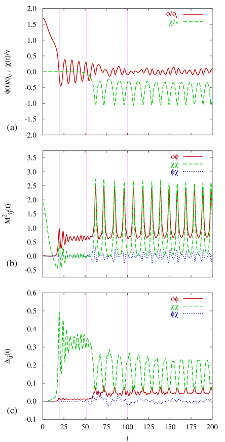
Figure 4: (Color online) Time evolution for the simulation with $g^{2}=2\lambda$. Initial values: $\phi(0)=1.2$ and $\chi(0)=1.0\times 10^{-7}$; other parameters: $m^{2}=0$, $\lambda=1$, $v^{2}=1$; we plot as a function of time (a) the classical fields $\phi(t)/\phi_{\mathrm{c}}$ (red solid line) and $\chi(t)/v$ (green dashed line), (b) the effective masses ${\cal M}^{2}_{ij}(t)$ with $ij={\phi\phi}$ (red solid line), $ij={\chi\chi}$ (green dashed line) and $ij={\phi\chi}$ (blue dotted line) (c) the fluctuation integrals $\Delta_{ij}(t)$ with $ij={\phi\phi}$ (red solid line), $ij={\chi\chi}$ (green dashed line) and $ij={\phi\chi}$ (blue dotted line); the vertical dotted lines indicate the times where $t$ is equal to $19.5$, $51.3$ and $100.2$

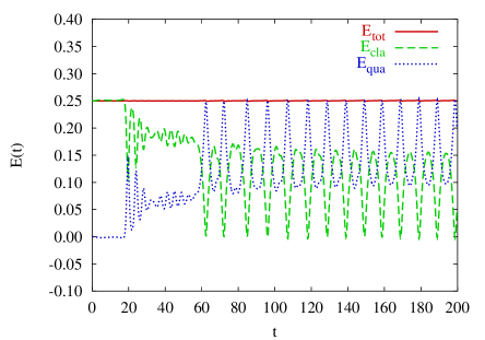
Figure 5: (Color online) Energy contributions for the simulation with parameters in Fig. 4; the red solid line denotes the total energy, the green dashed line the classical energy and the blue dotted line the quantum energy

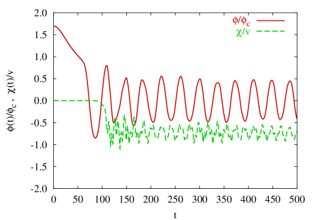
Figure 6: (Color online) The same as Fig. 4a but for the coupling case $g^{2}=0.1\lambda$ and the initial value $\phi(0)=5.366$

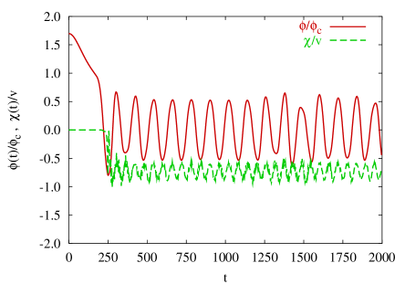
Figure 7: (Color online) The same as Fig. 4a but for the coupling case $g^{2}=0.01\lambda$ and the initial value $\phi(0)=16.97$

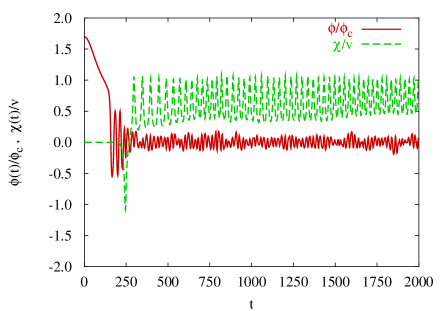
Figure 8: (Color online) The same as Fig. 4a but for $\lambda=0.1$

VII.2 Time regimes and exponential growth

We have identified three time regimes in the simulations that we want to investigate further in the following. The regimes are described as follows:

• Initial period, end of slow roll. Here ${\cal M}^{2}_{\chi\chi}(t)>0$. A phase of slow rolling of the inflaton field after the main period of inflation. The quantum fluctuations still are almost negligible.

• Early times, spinodal regime, ${\cal M}^{2}_{\chi\chi}(t)<0$ or oscillating several times around zero. Spinodal amplification of Higgs quantum fluctuations and and exponential growth of $\chi(t)$.

• Intermediate and late times, ${\cal M}^{2}_{\chi\chi}(t)>0$ and oscillations of the classical fields. Excitation of inflaton and mixed quantum fluctuations, parametric resonance bands in all momentum spectra.

The first period (I) is easy to identify in Figs. 4–6: only the inflaton decreases with time in smooth way while the Higgs mean field is still practically zero.

In the early time period (II) the inflaton field passes through zero once or several times, depending on the coupling $g^{2}$, see Figs. 4–7. The period is identified by an increase of $|\chi(t)|$ and ends once $\chi(t)$ begins to oscillate in a regular way. A closer analysis shows that the amplitude of the classical Higgs field growths exponentially. In Fig. 9 we display on a logarithmic scale the absolute value $|\chi(t)|$ for simulations with $g^{2}=2\lambda$, $\lambda=1$, $m^{2}=0$, $v^{2}=1$ and $\chi(0)=10^{-7}$ fixed, while the initial amplitude of the inflaton field, $\phi(0)$, is varied from $1.2$ to $1.8$. The exponential growth sets in when $\phi(t)$ becomes smaller than the critical value $\phi_{\mathrm{c}}$ (see Eq. (2.5)) and stops when $\chi(t)$ reaches the turning point which is at $|\chi(t)|\approx 1$. There does not seem to be a systematic trend for the dependence of the period of growth on $\phi(0)$.

The regime (II) can be very short. For the simulation with a small coupling $g^{2}=0.01\lambda$ the transition to the broken symmetry phase can take place within a single oscillation of the inflaton field (see Fig. 7a).

The intermediate and late time period (III) is characterized by oscillations of both the inflaton and the Higgs field, with essentially constant period and amplitude (see, e.g., Fig. 8). The Higgs mean field may oscillate around a nonzero value, related to a broken symmetry minimum of an effective potential (see below) or around $\chi=0$, to be identified with symmetry restoration. This period is further analyzed in the next subsection.

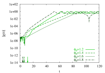
Figure 9: Time evolution of the absolute value $|\chi(t)|$ for simulations with the parameters $g^{2}=2\lambda$, $m^{2}=0$, $v^{2}=1$ and $\lambda=1$ and four different initial values $\phi(0)$ equal to $1.2$ (solid line), $1.4$ (dashed line), $1.6$ (dotted line) and $1.8$ (dashed-dotted line); the corresponding arrows pointing at the $t$-axis indicate the time when $\phi(t)$ drops below $\phi_{\mathrm{c}}$

VII.3 Late time averages – phase transition

The amplitudes of the classical fields $\phi$ and $\chi$ decrease very slowly, if at all, at late times, i.e., once they have started to oscillate in a kind of effective potential. Though we make no attempt to reconstruct such a potential in detail, the oscillations allow to conclude on the minimum and the range of such an effective potential for both the Higgs and inflaton fields. In this sense we can speak of a symmetric or broken symmetry phase for the Higgs field, if the minimum of its effective potential is at $\chi=0$ and $\chi\neq 0$, respectively, and we associate this minimum with the time average of the Higgs field at late times. The shape of the effective potential depends here on the energy density (in place of the temperature) and therefore on the initial value of the inflaton field. The question of spontaneous symmetry breaking and of the point of the phase transition reduces therefore to finding the the dependence of $\chi(t\to\infty)$ on the initial value $\phi(0)$.

In order to study this issue we have performed a series of simulations where we have varied the initial amplitude $\phi(0)$ while keeping all the other parameters fixed. In Fig. 10 the time evolution of $\chi(t)$ for simulations with $\phi(0)=1.9$, $2.0$ and $2.1$ is displayed. The other parameters are $g^{2}=2\lambda$, $\lambda=1$, $v=1$, $m=0$ and $\chi(0)=10^{-7}$.

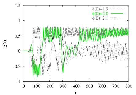
Figure 10: (Color online) Time evolution of $\chi(t)$ with parameters as in Fig. 9 but for the initial values $\phi(0)$ equal to $1.9$ (dashed line), $2.0$ (green solid line) and $2.1$ (dotted line).

A first inspection suggests that there is a phase transition between $\phi(0)=2.0$ and $\phi(0)=2.1$, as for the latter simulation the field $\chi$ oscillates around zero. From the simulation with $\phi(0)=2.0$ in Fig. 10 it becomes apparent that the field $\chi$ can jump several times from one “minimum” to the other if $\phi(0)$ is close to the critical point of the phase transition. This is typical for a first-order phase transition and has been observed in the scalar $O(N)$ model in the Hartree approximation as well Baacke:2001zt .

In Fig. 11 we display the time averages $|\overline{\chi}(\infty)|$ and $\overline{{\cal M}^{2}}_{\chi\chi}(\infty)$ as a function of the initial amplitude $\phi(0)$. The other parameters are fixed to $g^{2}=2\lambda$, $\lambda=1$, $v=1$, $m=0$ and $\chi(0)=10^{-7}$. A first-order phase transition is signaled by a non-continuous drop of the minimum value $|\overline{\chi}(\infty)|$ and the effective mass ${\cal M}^{2}_{\chi\chi}$ from finite (positive) values to zero.

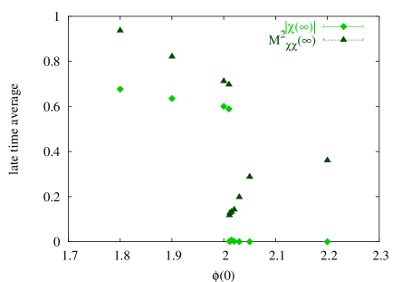
Figure 11: The late-time absolute value $|\chi(\infty)|$ (diamonds) and the late time effective mass ${\cal M}^{2}_{\chi\chi}(\infty)$ (triangles) averaged at times $t\approx 1000$ as a function of the initial amplitude $\phi(0)$; other parameters as in Fig. 4.

VII.4 Momentum spectra

Using the amplitudes $f_{j}^{\alpha}(t,p)$ one may define various “power spectra”. One of those is the integrand of the fluctuation integrals $\Delta_{ij}(t)$, i.e., the tadpole contributions. We have already introduced the kernel

$$G_{ij}(t,t,{\bf p})=\langle\tilde{\Phi}^{*}_{i}(t,{\bf p})\tilde{\Phi}(t,{\bf p})\rangle/V$$ (7.39)

in terms of which we define the power spectrum of the fluctuation amplitudes

$$P_{ij}(t,p)=G_{ij}(t,t,{\bf p})\frac{p^{2}}{2\pi^{2}}$$ (7.40)

by including the momentum phase space factor.

In Fig. 12 we display this spectrum for the simulation in Fig. 4 at the times $t$ equal to $19.5$, $51.3$ and $100.2$. These time steps are indicated in Fig. 4 by vertical dashed lines. Actually we have subtracted the free field part and the first order perturbative part of this kernel, in analogy to the right hand side of Eq. (V.2). The free field part rises linearly with momentum; for $p=2$, the maximal value used in our plots, it is has typical values of $0.05$ and would be visible. It makes the tadpole integrals divergent; as discussed above, in our computations this divergence is absorbed by dimensional regularization and renormalization.

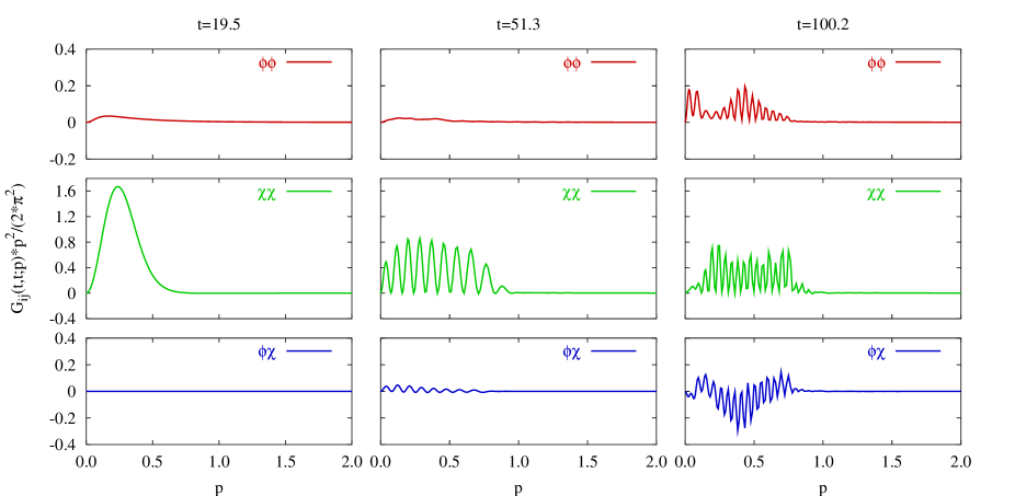
Figure 12: Momentum spectra $G_{ij}(t,t;\mathbf{p})p^{2}/(2\pi^{2})$ for the simulation in Fig. 4 at the times $t=19.5$ (left), $t=51.3$ (middle) and $t=100.2$ (right)

At early and intermediate times the Higgs fluctuations dominate. The inflaton and mixed fluctuation spectra only appear in the late-time regime, are however subdominant even there. At early times, $t<20$ the Higgs spectrum is generated by negative squared masses as in tachyonic preheating or quench scenarios. In Ref. Garcia-Bellido:2002aj it was found that the peak in the momentum spectrum $pP_{\chi\chi}(t,p)$ can be fitted by a Gaussian; we similarly find, at $t=19.5$, a spectrum

$$pP_{\chi\chi}(t,p)\simeq A\exp\left[-B(|\mathbf{p}|-C)^{2}\right]$$ (7.41)

with

$$A = 0.4482\pm 0.0038$$ (7.42)

$$B = 36.1115\pm 0.7131$$ (7.43)

$$C = 0.307995\pm 0.001168$$ (7.44)

At intermediate times the smooth peak broadens and decays into spikes, typical of parametric resonance. Parametric resonance also dominates the shape of the spectra at late times. As the period and amplitude of oscillation change very slowly, the width of the spectrum remains constant.

VII.5 Correlations

We define the correlation function between the different fluctuations as

$$C_{ij}(r,t) = \int\frac{d^{3}p}{(2\pi)^{3}}e^{i{\bf p}\cdot\mathbf{x}}\sum_{\alpha}\frac{1}{2\omega_{\alpha}}\textrm{Re}\,\left(f_{i}^{\alpha}(t,p)f_{j}^{*\,\alpha}(t,p)\right)$$ (7.45)

$$= \frac{1}{2\pi^{2}\,r}\int_{0}^{\infty}dpp\sin(pr)$$

$$\quad\times\sum_{\alpha}\frac{1}{2\omega_{\alpha}}\textrm{Re}\,\left(f_{i}^{\alpha}(t,p)f_{j}^{*\,\alpha}(t,p)\right)\;.$$

We here consider the correlations of the Higgs fluctuations ($i=j=2$), which are displayed in Fig. 13. We observe the correlations to be positive and propagating with $\Delta r=2\Delta t$, as also found in the large-$N$ approximation Boyanovsky:1998yp . The propagation with twice the speed of light can be related to the fact that the quantum fluctuations are correlated by the mean fields whose influence propagates in opposite space directions. This is corroborated by a strong decrease of such correlations when the mean field amplitude goes to zero Baacke:2001zt .

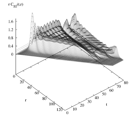
Figure 13: Correlation function $rC_{\chi\chi}(r,t)$ for the simulation in Fig. 4

VII.6 Decoherence time

One of the important questions is the justification of using classical instead of quantum dynamics. In the context of nonequilibrium quantum field theory this has been discussed in Refs. Guth:1985ya ; Polarski:1996jg ; Khlebnikov:1996mc and applied to the hybrid model in Refs. Asaka:2001ez ; Garcia-Bellido:2002aj . We use here, adapted to our normalization, the definitions of Ref. Garcia-Bellido:2002aj . The “classicality” is measured by the imaginary part $F(t,{\bf p})$ of a correlation function:

$$F_{ij}(t,{\bf p})={\rm Im}\left[\sum_{\alpha}\frac{f_{i}^{\alpha*}(t,p)\dot{f}_{j}^{\alpha}(t,p)}{2\omega_{\alpha}}\right]$$ (7.46)

the real part of the bracket being associated with the commutator. The criterium for a classical description is given by

$$|F_{ii}|\gg 1\;.$$ (7.47)

We display in Fig. 14 the time for the onset of classicality (“decoherence time”) as a function of momentum.

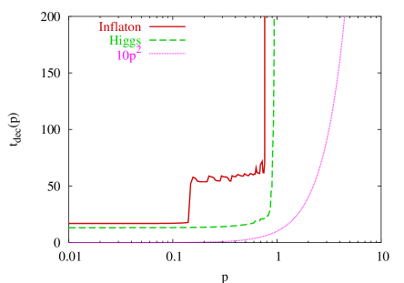
Figure 14: (Color online) Decoherence time $t_{\mathrm{dec}}(p)$ for which a given mode $p$ becomes “classical” ($|F_{ij}(t_{\mathrm{dec}},{\bf p})|=1$) for the simulation in Fig. 4; the red solid line represents the inflaton ($i=j=1$) and the green dashed line the Higgs modes ($i=j=2$); the dotted line corresponds to $t_{\mathrm{dec}}\propto p^{2}$.

As far as the Higgs fluctuations ($i=j=2$) are concerned the figure can be compared to those of Refs. Asaka:2001ez ; Garcia-Bellido:2002aj . These authors consider the creation of quantum fluctuations via the spinodal instability. They simplify the time evolution by assuming for the mass of the Higgs fluctuations a behavior ${\cal M}^{2}_{\chi\chi}\propto(t_{0}-t)$ where $t_{0}$ marks the onset of the spinodal regime, without considering any back reactions (see also Refs Guth:1985ya ; Bowick:1998kd ; Copeland:2002ku ; Lombardo:2002wt ). In this case the mode functions become Airy functions and the results are in analytic form. The boundary $|F(t,{\bf p})|=1$ between the classical and quantum regimes then behaves roughly Garcia-Bellido:2002aj as $t\propto{\bf p}^{2}$. As displayed in Fig. 14 the shape of this boundary is quite different in our simulations, the classical regimes remains limited within a fixed momentum band at all times. When one includes back reaction the behavior of the mass term is linear in time only in a very limited time interval; furthermore, due to the inflaton oscillations, the process repeats several times. The limited momentum band for which the modes can be considered as classical, can be seen as a consequence of parametric resonance. Due to the lack of strong dissipation the oscillations of the classical fields persist at late times, and therefore also the resonance band. Whether and for which time period this is physical or unphysical cannot be determined within the approximation used here, even though it is certainly more elaborate as previous approaches.

For the inflaton fluctuations, not considered in Ref.Asaka:2001ez ; Garcia-Bellido:2002aj , the structure of this curve shows that fluctuations at very small momenta become classical as early as those of the Higgs field, while those for larger momenta develop at later times. This is due, presumably, to a stronger role of parametric resonance for the evolution of inflaton fluctuations. Again the band of momenta for the classical regime remains sharply cutoff even at late times.

VIII Conclusions

In this final section we would like to comment on some of our results and draw some conclusions.

On the formal level we have addressed the problem of renormalization for a fully coupled system of two quantum fields in the Hartree approximation, using methods similar to those in Refs. Cormier:2001iw ,Baacke:1997kj and Baacke:2001zt , but going beyond these applications. We consider this as an essential achievement of our work, which will important when extending the model by including Goldstone and gauge fields and the coupling to gravity where proper renormalization is indispensable Baacke:1999gc . Nevertheless we do not want to infer that working with judiciously chosen cutoffs or less elaborate schemes one may not reach sensible physical insights.

When treated in the Hartree approximation this model lacks an efficient mechanism for dissipation. This is considered to be a general drawback of the Hartree approximation. The situation would improve, however, even in this approximation, if Goldstone modes were included (see, e.g. Fig. 1 in Ref. Baacke:2001zt ). Dissipation via particle production is also found in the large-$N$ limit Boyanovsky:1995me . In more realistic models dissipation may proceed in addition via fermion and gauge fields. The higher order effects (sunset graphs or NLO-1/N) become effective only when quantum fluctuations have grown to sufficient size. This depends of course on the parameters of the model. In the earlier stages the Hartree approximation should be able to provide reliable information on the evolution of decay and resonance processes. The time scales for thermalization are expected to be much larger.

The model displays the expected transition to a broken symmetry phase if the initial inflaton amplitude is not too large. A possible intermediate restoration of symmetry by quantum fluctuations would be followed by a later transition to the broken symmetry state after further cosmological expansion. Possible consequences like the unwanted formation of topological defects have been discussed in the literature Khlebnikov:1998sz:Parry:1998de .

We have calculated the boundaries between regions where a quantum description is needed and those where one may have recurse to classical evolution equations. We find marked differences with respect to previous work Asaka:2001ez ; Garcia-Bellido:2002aj , where the production of quanta is described in a simplified way, using a squared mass of the Higgs field passing linearly through zero. We find numerically that the back reaction limits the classical regime to a low-momentum region fixed for all times. Though large excitations of quantum fluctuations seem to justify the transition to a classical description one has to keep in mind, that finally one wants to end up with an ensemble described by quantum statistics which is used in the standard thermal history of the early universe. The classical ensembles suffer from the Rayleigh-Jeans divergence incompatible with the finite amount of initial energy density. This automatically forces the fluctuations back to the quantum regime.

The model discussed here corresponds to the original proposal by Linde, using a double well potential. This has been used, as a simplification or a generic feature in some previous studies Asaka:2001ez . For electroweak or GUT scale preheating the Higgs sector is based on a symmetry group like $SU(n)$ or $SO(n)$ and will in general have more ($n_{H}$) degrees of freedom. Near the spinodal point their masses are degenerate, and this fact has been used in some studies Garcia-Bellido:2002aj in the way of just using $n_{H}$ identical copies of one and the same degree of freedom. However, once the mean value of the Higgs field departs from zero, there will be a nontrivial mass matrix for the quantum fluctuations with several massless degrees of freedom, the would-be Goldstone bosons. It can be expected that this will modify the quantum back reaction in an essential way. While this goes beyond the scope of the present investigation, there are some studies using classical dynamics with more realistic Higgs sectors Felder:2001kt ; Felder:2000hj ; Borsanyi:2002tm:Borsanyi:2003ib . Our formalism allows for a generalization towards more realistic Higgs sectors, albeit with the limitation of homogeneous background fields.

To become even more realistic, in particular in view of low scale inflation, it would be very desirable to include gauge fields as well. Unfortunately any resummation or backreaction introduces gauge parameter dependences Baacke:1999sc ; Heitmann:2001qt , which are poorely understood in the framework of nonequilibrium quantum field theory. There is some recent progress in this direction Arrizabalaga:2002hn ; Mottola:2003vx ; Carrington:2003ut , however not yet on the level of concrete simulations.

Appendix A Identities for Feynman integrals

Within dimensional regularization ($D=4-\epsilon$) the following identities (no summation over Greek indices) hold

$$\int\frac{d^{D-1}p}{(2\pi)^{D-1}}\frac{1}{2\omega_{\alpha}\omega_{\beta}(\omega_{\alpha}+\omega_{\beta})}$$

$$=\int\frac{d^{D}p}{(2\pi)^{D}}\frac{1}{(p^{2}-m_{0,\,\alpha}^{2}+io)(p^{2}-m_{0,\,\beta}^{2}+io)}$$ (A48)

$$=\frac{1}{16\pi^{2}}\left[L_{\epsilon}-\ln\frac{m_{0,\,\alpha}^{2}}{\mu^{2}}+1+\frac{m_{0,\,\beta}^{2}}{m_{0,\,\alpha}^{2}-m_{0,\,\beta}^{2}}\ln\frac{m_{0,\,\beta}^{2}}{m_{0,\,\alpha}^{2}}\right]$$

and

$$\int\frac{d^{D-1}p}{(2\pi)^{D-1}}\frac{1}{2\omega_{\alpha}} = \int\frac{d^{D}p}{(2\pi)^{D}}\frac{i}{p^{2}-m_{0,\,\alpha}^{2}+io}$$ (A50)

$$= \,-\frac{m_{0,\,\alpha}^{2}}{16\pi^{2}}\left[L_{\epsilon}-\ln\frac{m_{0,\,\alpha}^{2}}{\mu^{2}}+1\right]\quad$$ (A51)

with

$$\omega_{\alpha} = \sqrt{m_{0,\,\alpha}^{2}+\mathbf{p}^{2}}$$ (A52)

$$L_{\epsilon} = \frac{2}{\epsilon}-\gamma+\ln 4\pi\ .$$ (A53)

The corresponding Feynman diagrams are depicted in Fig. 15. Note that

$$\lim_{m_{0,\,\beta}^{2}\to\,m_{0,\,\alpha}^{2}}\!\!\! \!\!\!\left[-\ln\frac{m_{0,\,\alpha}^{2}}{\mu^{2}}+1+\frac{m_{0,\,\beta}^{2}}{m_{0,\,\alpha}^{2}-m_{0,\,\beta}^{2}}\ln\frac{m_{0,\,\beta}^{2}}{m_{0,\,\alpha}^{2}}\right]$$ (A54)

$$=-\ln\frac{m_{0,\,\alpha}^{2}}{\mu^{2}}\ .$$

(a)           (b)

Figure 15: (a) The Feynman diagram with a topology of a fish graph corresponding to Eq. (A48) (b) the tadpole type graph corresponding to Eq. (A51); in both diagrams the lines denote free propagators with the initial masses $m_{0,\,\alpha}^{2}$ and $m_{0,\,\beta}^{2}$, respectively

An identity that is needed for the renormalization of the energy is given by

$$\int\frac{d^{D-1}p}{(2\pi)^{D-1}}\omega_{\alpha}=\,\frac{m_{0,\,\alpha}^{4}}{32\pi^{2}}\left[L_{\epsilon}-\ln\frac{m_{0,\,\alpha}^{2}}{\mu^{2}}+\frac{3}{2}\right]\ .$$ (A55)

Appendix B Perturbative expansion of the mode functions

We will present in this section the isolation of the divergences via a perturbative expansion of the mode functions (see e.g. Ref. Baacke:1997se ; Baacke:1997kj ) for the case of a coupled system of equations.

Let us split the mode functions $f_{i}^{\alpha}$ into a free part containing the initial matrix $O_{ij}$ and higher order terms represented by the reduced mode functions $h_{i}^{\alpha}$, i.e.

$$f_{i}^{\alpha}(t;p) = e^{-i\omega_{\alpha}t}\left[O_{i\alpha}+h_{i}^{\alpha}(t;p)\right]\ .$$ (B56)

Here and in the following no summation over Greek indices is meant if not explicitly stated.

If we define a potential

$$\mathcal{V}_{ij}(t) = {\cal M}^{2}_{ij}(t)-{\cal M}^{2}_{ij}(0)\$$ (B57)

the differential equation (3.40) is equivalent to the following integral equation

$$f_{i}^{\alpha}(t;p) = e^{-i\omega_{\alpha}t}O_{i\alpha}$$

$$+\int_{0}^{t}{dt^{\prime}\,}K^{\mathrm{ret}}_{ij}(t-t^{\prime};p)\mathcal{V}_{jk}(t^{\prime})f_{k}^{\alpha}(t^{\prime};p)\ .$$

The retarded kernel of the free equation is given by

$$K^{\mathrm{ret}}_{ij}(t-t^{\prime};p) = \sum_{\beta}\frac{i}{2\omega_{\beta}}\Theta(t-t^{\prime})O_{i\beta}O_{j\beta}$$ (B58)

$$\times\left[e^{i\omega_{\beta}(t-t^{\prime})}-e^{-i\omega_{\beta}(t-t^{\prime})}\right]\ .$$

Inserting the retarded kernel in the integral equation gives

$$f_{i}^{\alpha}(t;p) = e^{-i\omega_{\alpha}t}O_{i\alpha}$$ (B59)

$$+\int_{0}^{t}{dt^{\prime}\,}\sum_{\beta}\frac{i}{2\omega_{\beta}}O_{i\beta}O_{j\beta}$$

$$\times\left[e^{i\omega_{\beta}(t-t^{\prime})}-e^{-i\omega_{\beta}(t-t^{\prime})}\right]$$

$$\times\mathcal{V}_{jk}(t^{\prime})f_{k}^{\alpha}(t^{\prime};p)$$

$$= e^{-i\omega_{\alpha}t}\bigg{\{}O_{i\alpha}+\int_{0}^{t}{dt^{\prime}\,}\mathcal{V}_{jk}(t^{\prime})$$ (B61)

$$\qquad\quad\times\sum_{\beta}\frac{i}{2\omega_{\beta}}O_{i\beta}O_{j\beta}O_{k\alpha}$$

$$\quad\times\bigg{[}e^{i(\omega_{\beta}+\omega_{\alpha})(t-t^{\prime})}$$

$$\qquad\quad-e^{-i(\omega_{\beta}-\omega_{\alpha})(t-t^{\prime})}\bigg{]}\bigg{\}}$$

$$+\ldots\ ,$$

where in addition the decomposition in Eq. (B56) has been used. The dots imply the higher order terms with $h_{i}^{\alpha}$ that we do not need for the analysis of the divergences here.

By partial integration the divergent contributions can be isolated in the usual manner

$$f_{i}^{\alpha}(t;\mathbf{p}) = e^{-i\omega_{\alpha}t}\bigg{\{}O_{i\alpha}$$

$$\quad-\sum_{\beta}\frac{1}{2\omega_{\beta}}\left[\frac{1}{\omega_{\beta}+\omega_{\alpha}}+\frac{1}{\omega_{\beta}-\omega_{\alpha}}\right]$$

$$\quad\times O_{i\beta}O_{j\beta}O_{k\alpha}\mathcal{V}_{jk}(t)$$

$$\quad+\sum_{\beta}\frac{1}{2\omega_{\beta}}\bigg{[}\frac{1}{\omega_{\beta}+\omega_{\alpha}}e^{i(\omega_{\beta}+\omega_{\alpha})t}$$

$$\quad+\frac{1}{\omega_{\beta}-\omega_{\alpha}}e^{-i(\omega_{\beta}-\omega_{\alpha})t}\bigg{]}$$

$$\quad\times O_{i\beta}O_{j\beta}O_{k\alpha}\mathcal{V}_{jk}(0)$$

$$\quad+\sum_{\beta}\frac{1}{2\omega_{\beta}}O_{i\beta}O_{j\beta}O_{k\alpha}$$

$$\quad\times\int_{0}^{t}dt^{\prime}\dot{\mathcal{V}}_{jk}(t^{\prime})\bigg{[}\frac{1}{\omega_{\beta}+\omega_{\alpha}}e^{i(\omega_{\beta}+\omega_{\alpha})(t-t^{\prime})}$$

$$\qquad+\frac{1}{\omega_{\beta}-\omega_{\alpha}}e^{-i(\omega_{\beta}-\omega_{\alpha})(t-t^{\prime})}\bigg{]}\bigg{\}}$$

$$+\ldots\ .$$

This expression and its complex conjugate is all what is needed to calculate the divergent contributions in $\Delta_{ij}(t)$. We have for the divergent part of the symmetrized Green’s function

$$\frac{1}{2}\bigg{[}G_{ij}(t,t;\mathbf{p})+G_{ji}(t,t;\mathbf{p})\bigg{]}^{\mathrm{div}}$$

$$=\sum_{\alpha}\frac{1}{2\omega_{\alpha}}\mathrm{Re}\bigg{[}f_{i}^{\alpha}(t;p)f_{j}^{\alpha,\,*}(t;p)\bigg{]}^{\mathrm{div}}$$

$$=\sum_{\alpha}\frac{1}{2\omega_{\alpha}}\bigg{[}O_{i\alpha}O_{j\alpha}$$

$$\qquad+\sum_{\beta}\frac{1}{2\omega_{\beta}}O_{i\beta}O_{l\beta}O_{k\alpha}O_{j\alpha}\mathcal{V}_{kl}(t)\frac{-2\omega_{\beta}}{\omega_{\beta}^{2}-\omega_{\alpha}^{2}}$$

$$\qquad+\sum_{\beta}\frac{1}{2\omega_{\beta}}O_{i\alpha}O_{l\beta}O_{k\alpha}O_{j\beta}\mathcal{V}_{kl}(t)\frac{-2\omega_{\beta}}{\omega_{\beta}^{2}-\omega_{\alpha}^{2}}\bigg{]}$$

$$=\sum_{\alpha}\frac{1}{2\omega_{\alpha}}\bigg{[}O_{i\alpha}O_{j\alpha}$$

$$\qquad-\frac{1}{\omega_{\beta}(\omega_{\alpha}+\omega_{\beta})}O_{i\alpha}O_{j\beta}O_{l\beta}O_{k\alpha}\mathcal{V}_{kl}(t)\bigg{]}\ .$$ (B63)

These expressions become divergent if they are integrated over $d^{3}p$. We will use them as subtraction terms in the fluctuation integrals in $\Delta^{(1)}_{ij}(t)$ and $E^{(1)}(t)$ [see Eqs. (IV) and (4.9)].

The divergences in the energy can be found in an analogous way by inserting $f_{i}^{\alpha}(t,p)$ and its time derivative in the one-loop energy part $E^{(1)}(t)$ [see Eq. (4.9)]. We will use an alternative approach in the following.

The one-loop effective action at time $t$ minus the one at $t=0$ is given by

$$\widetilde{\Gamma}^{(1)}[{\cal M}^{2}]=\frac{i}{2}{\rm Tr}\ln\left\{\frac{\Box+{\cal M}^{2}(t)}{\Box+{\cal M}^{2}(0)}\right\}$$ (B64)

where it is understood that the numerator and denominator are $2\times 2$ matrices. This expression can be expanded locally with respect to ${\cal V}={\cal M}^{2}(t)-{\cal M}^{2}(0)$ and gradients thereof. The expansion can be obtained by going to the momentum representation and by expanding with respect to insertions of ${\cal V}(q)$ and with respect to the external momenta $q=(q_{0},\mathbf{q})$. As we do not need an infinite wave function renormalization the divergent parts are given by the terms of first and second order in ${\cal V}(q)$.

We introduce

$$G_{0,ij}^{-1}(p) = \left(-p_{0}^{2}+{\bf p}^{2}\right)\delta_{ij}+m^{2}_{0,ij}$$ (B65)

$$G_{ij}^{-1}(p) = \left(-p_{0}^{2}+{\bf p}^{2}\right)\delta_{ij}+{\cal M}^{2}_{ij}(t)$$ (B66)

with $m^{2}_{0,ij}={\cal M}^{2}_{ij}(0)$. $G_{0}$ is not the bare propagator which would be defined at the vacuum expectation values of $\phi$ and $\chi$. We diagonalize the initial mass matrix by an orthogonal transformation

$${\cal M}^{2}(0)=O\widetilde{\cal M}^{2}(0)O^{T}$$ (B67)

or

$$m^{2}_{0,ij}=O_{i\alpha}O_{j\beta}\widetilde{m}^{2}_{0,\alpha\beta}=O_{i\alpha}O_{j\alpha}\widetilde{m}^{2}_{0,\alpha}\;.$$ (B68)

Then also $G_{0,ij}^{-1}$ becomes diagonal. The same holds true for the inverse matrix. We likewise introduce

$$G_{ij}^{-1}(p) = O_{i\alpha}\left(\left[-p_{0}^{2}+{\bf p}^{2}+\widetilde{m}^{2}_{0,\alpha}\right]\delta_{\alpha\beta}+\widetilde{\cal V}_{\alpha\beta}(t)\right)O_{j\beta}$$ (B69)

$$= O_{i\alpha}\widetilde{G}_{\alpha\beta}^{-1}(p)O_{j\beta}\ ,$$

where of course

$$\widetilde{\cal V}_{\alpha\beta}(t)=O_{i\alpha}{\cal V}_{ij}(t)O_{j\beta}$$ (B70)

is no longer diagonal. The effective action, in the approximation where all gradient terms are neglected, can now be rewritten as

$$\widetilde{\Gamma}^{(1)} \simeq \frac{i}{2}\int\frac{d^{4}p}{(2\pi)^{4}}{\rm Tr}\ln\left\{G_{0}G^{-1}\right\}$$ (B71)

$$= \int\frac{d^{4}p}{(2\pi)^{4}}{\rm Tr}\ln\left\{1+\widetilde{G}_{0}\widetilde{\cal V}(t)\right\}\;.$$

The first terms in the expansion are

$$\widetilde{\Gamma^{(1)}} \simeq \frac{i}{2}\int\frac{d^{4}p}{(2\pi)^{4}}\left[\sum_{\alpha}\frac{1}{-p_{0}^{2}+{\bf p}^{2}+m^{2}_{0,\alpha}+io}\widetilde{\cal V}_{\alpha\alpha}(t)\right.$$ (B72)

$$-\frac{1}{2}\sum_{\alpha\beta}\frac{1}{-p_{0}^{2}+{\bf p}^{2}+m^{2}_{0,\alpha}+io}\widetilde{\cal V}_{\alpha\beta}(t)$$

$$\times\left.\frac{1}{-p_{0}^{2}+{\bf p}^{2}+m^{2}_{0,\beta}+io}\widetilde{\cal V}_{\beta\alpha}(t)\right]$$

$$+O(\widetilde{\cal V}^{3})$$

The three-dimensional reduction is obtained via Eq. (A51) and Eq. (A48). So we find

$$\widetilde{\Gamma}^{(1)\,{\rm div}} = \int\frac{d^{3}p}{(2\pi)^{3}}\bigg{[}\sum_{\alpha}\frac{-\widetilde{\cal V}_{\alpha\alpha}(t)}{4\omega_{\alpha}}$$ (B73)

$$-\frac{1}{2}\sum_{\alpha\beta}\frac{-\widetilde{\cal V}_{\alpha\beta}(t)\widetilde{\cal V}_{\beta\alpha}(t)}{4\omega_{\alpha}\omega_{\beta}(\omega_{\alpha}+\omega_{\beta})}\bigg{]}\ .$$

The divergent parts of the fluctuation energy are, therefore,

$$E^{(1)}_{\rm div}=\int\frac{d^{3}p}{(2\pi)^{3}}\left[\sum_{\alpha}\frac{\widetilde{\cal V}_{\alpha\alpha}(t)}{4\omega_{\alpha}}-\sum_{\alpha\beta}\frac{\widetilde{\cal V}_{\alpha\beta}(t)\widetilde{\cal V}_{\beta\alpha}(t)}{8\omega_{\alpha}\omega_{\beta}(\omega_{\alpha}+\omega_{\beta})}\right]\ .\$$ (B74)

As a cross check we may obtain the divergent terms in the fluctuation integrals $\Delta_{ij}$ which are given by

$$\frac{\Delta^{(1)\,\rm div}_{ij}}{2}=-\frac{\delta\widetilde{\Gamma}^{(1)\,\rm div}}{\delta{\cal M}^{2}_{ij}(t)}=-\frac{\delta\widetilde{\Gamma}^{(1)\,\rm div}}{\delta{\cal V}_{ij}(t)}$$ (B75)

Using Eq. (B70) we have

$$\frac{\delta{\cal V}_{\alpha\beta}(t)}{\delta{\cal V}_{ij}(t)}=O_{i\alpha}O_{j\beta}$$ (B76)

and therefore

$$\Delta^{(1)\,\rm div}_{ij} = \int\frac{d^{3}p}{(2\pi)^{3}}\bigg{[}\sum_{\alpha}\frac{1}{2\omega_{\alpha}}O_{i\alpha}O_{j\alpha}$$ (B77)

$$-\sum_{\alpha\beta}\frac{O_{i\alpha}O_{j\beta}\widetilde{\cal V}_{\beta\alpha}(t)}{2\omega_{\alpha}\omega_{\beta}(\omega_{\alpha}+\omega_{\beta})}\bigg{]}\ .$$

Appendix C Counterterm structure

In this appendix we will establish a connection between the effective counterterms used above and the counterterms in the 2PPI formalism. The latter ones follow from a standard counterterm Lagrangian. For details we refer the reader to Ref. Verschelde:1992bs:Coppens:1993zc ; Verschelde:2000ta ; Verschelde:2000dz .

The general Lagrange density for the model in Eq. (3.7) including a counterterm $\delta\mathcal{L}$ denotes

$${\cal L} = \frac{1}{2}\partial_{\mu}\Phi^{i}\partial^{\mu}\Phi^{i}-\frac{1}{2}m_{ij}^{2}\Phi^{i}\Phi^{j}-\frac{1}{4!}\lambda_{ijkl}\Phi^{i}\Phi^{j}\Phi^{k}\Phi^{l}$$ (C78)

$$+\delta{\cal L}\ .$$

The counterterm Lagrangian $\delta\mathcal{L}$ is given by

$$\delta{\cal L} = \frac{1}{2}\delta Z_{ij}\partial^{\mu}\Phi^{i}\partial^{\mu}\Phi^{j}-\frac{1}{2}\delta m_{ij}^{2}\Phi^{i}\Phi^{j}$$ (C79)

$$-\frac{1}{4!}\delta\lambda_{ijkl}\Phi^{i}\Phi^{j}\Phi^{k}\Phi^{l}\ .$$

The gap equation for the renormalized effective mass ${\cal M}^{2}_{\mathrm{R},\,ij}$ with mass and coupling constant counterterms is given by

$${\cal M}^{2}_{\mathrm{R},\,ij} = m_{ij}^{2}+\delta m_{ij}^{2}$$ (C80)

$$+\frac{1}{2}(\lambda_{ijkl}+\delta\lambda_{ijkl})\left(\phi^{k}\phi^{l}+\Delta^{kl}\right)\ .$$

In the 2PPI scheme the following relations for the renormalization constants hold, if one takes a mass independent renormalization scheme

$$(\delta m^{2})^{ij} = \delta Z_{m}^{ij;kl}m_{kl}^{2}$$ (C81)

$$\delta\lambda^{ij;kl} = \lambda^{ij}_{\ \ pq}\delta Z_{m}^{\,pq;kl}$$ (C82)

$$\delta Z_{m}^{\,ij;kl} = \lambda^{ij}_{\ \ pq}\delta\zeta^{pq;kl}\ .$$ (C83)

Thus all renormalization constants can be derived from a vacuum counter term

$$\delta E_{\mathrm{vac}} = \frac{1}{2}{\cal M}^{2}_{ij}{\cal M}^{2}_{kl}\,\delta\zeta^{ij;kl}\ .$$ (C84)

With the help of these identities the gap equation reads

$${\cal M}^{2}_{\mathrm{R},\,ij} = m_{ij}^{2}+\frac{1}{2}\lambda_{ijkl}\left(\phi^{k}\phi^{l}+\Delta^{kl}\right)$$ (C85)

$$+\lambda_{ijpq}\,\delta\zeta^{pq;kl}m_{kl}^{2}$$

$$+\frac{1}{2}\lambda_{ijpq}\lambda^{pqrs}\,\delta\zeta_{rs;kl}\left(\phi^{k}\phi^{l}+\Delta^{kl}\right)$$

$$= m_{ij}^{2}+\frac{1}{2}\lambda_{ijkl}\left(\phi^{k}\phi^{l}+\Delta^{kl}_{\mathrm{R}}\right)\ ,$$ (C86)

with

$$\lambda_{ijkl}\Delta^{kl}_{\mathrm{R}} = \lambda_{ijkl}\Delta^{kl}+2\lambda_{ijpq}\delta\zeta^{pq;kl}m_{kl}^{2}$$ (C87)

$$+\frac{1}{2}\lambda_{ijpq}\lambda^{pqrs}\,\delta\zeta_{rs;kl}\left(\phi^{k}\phi^{l}+\Delta^{kl}\right)\ .$$

Once the propagator $\Delta^{ij}$ is renormalized the gap equations for the masses ${\cal M}^{2}_{ij}$ become finite. In the Hartree approximation, i.e. the one-loop 2PPI approximation, the equations for the classical fields $\phi^{i}$ are finite as well. No wave function renormalization is needed.

If we specialize Eq. (C87) with the help of Eq. (3.9)–(3.16) to our given hybrid model, the renormalization constants $\delta\zeta$ simplify to

$$\delta\zeta_{\phi\phi;\phi\phi} = \delta\zeta_{\chi\chi;\chi\chi}=:-2\delta\xi_{\phi\phi}=-2\delta\xi_{\chi\chi}$$ (C88)

$$\delta\zeta_{\phi\chi;\phi\chi} = \delta\zeta_{\chi\phi;\chi\phi}=:-2\delta\xi_{\phi\chi}$$ (C89)

$$\delta\zeta_{\phi\phi;\chi\chi} = \delta\zeta_{\phi\chi;\phi\phi}=\ldots=0\ .$$ (C90)

The vacuum counter term in Eq. (C84) reduces to

$$\delta E_{\mathrm{vac}} = -\delta\xi_{\phi\phi}({\cal M}^{2}_{\phi\phi})^{2}-\delta\xi_{\chi\chi}({\cal M}^{2}_{\chi\chi})^{2}-2\delta\xi_{\phi\chi}({\cal M}^{2}_{\phi\chi})^{2}$$ (C91)

$$= -\delta{\cal M}^{4}\ .$$

Thus the effective counterterm $\delta{\cal M}^{4}$ used in Sec. V.3 has been mapped to the renormalization constants of a standard counterterm Lagrangian $\delta\mathcal{L}$ [see Eq. (C79)]. In principle one can calculate the nonperturbatively fixed counterterms $\delta m^{2}$, $\delta v^{2}$, $\delta g^{2}$ and $\delta\lambda$ explicitly, insofar the renormalized gap equations form a coupled system of equations. However, this would not be very enlightening.

References

- (1) A. D. Linde, Phys. Lett. B249, 18 (1990).
- (2) A. D. Linde, Phys. Lett. B259, 38 (1991).
- (3) A. D. Linde, Phys. Rev. D49, 748 (1994), [astro-ph/9307002].
- (4) E. J. Copeland, A. R. Liddle, D. H. Lyth, E. D. Stewart and D. Wands, Phys. Rev. D49, 6410 (1994), [astro-ph/9401011].
- (5) J. Garcia-Bellido and A. D. Linde, Phys. Rev. D 57, 6057 (1998), [hep-ph/9711360].
- (6) R. Micha and M. G. Schmidt, Eur. Phys. J. C14, 547 (2000), [hep-ph/9908228].
- (7) W. Buchmuller, L. Covi and D. Delepine, Phys. Lett. B491, 183 (2000), [hep-ph/0006168].
- (8) H. P. Nilles, M. Peloso and L. Sorbo, JHEP 04, 004 (2001), [hep-th/0103202].
- (9) T. Asaka, W. Buchmuller and L. Covi, Phys. Lett. B510, 271 (2001), [hep-ph/0104037].
- (10) D. Cormier, K. Heitmann and A. Mazumdar, Phys. Rev. D65, 083521 (2002), [hep-ph/0105236].
- (11) D. H. Lyth and A. Riotto, Phys. Rept. 314, 1 (1999), [hep-ph/9807278].
- (12) J. Garcia-Bellido, D. Y. Grigoriev, A. Kusenko and M. E. Shaposhnikov, Phys. Rev. D60, 123504 (1999), [hep-ph/9902449].
- (13) M. Bastero-Gil, S. F. King and J. Sanderson, Phys. Rev. D60, 103517 (1999), [hep-ph/9904315].
- (14) L. M. Krauss and M. Trodden, Phys. Rev. Lett. 83, 1502 (1999), [hep-ph/9902420].
- (15) G. N. Felder et al., Phys. Rev. Lett. 87, 011601 (2001), [hep-ph/0012142].
- (16) G. N. Felder, L. Kofman and A. D. Linde, Phys. Rev. D64, 123517 (2001), [hep-th/0106179].
- (17) E. J. Copeland, D. Lyth, A. Rajantie and M. Trodden, Phys. Rev. D64, 043506 (2001), [hep-ph/0103231].
- (18) J. Garcia-Bellido, M. Garcia Perez and A. Gonzalez-Arroyo, Phys. Rev. D67, 103501 (2003), [hep-ph/0208228].
- (19) S. Borsanyi, A. Patkos and D. Sexty, Phys. Rev. D66, 025014 (2002), [hep-ph/0203133]; S. Borsanyi, A. Patkos and D. Sexty, Phys. Rev. D68, 063512 (2003), [hep-ph/0303147].
- (20) D. Boyanovsky, D. Cormier, H. J. de Vega and R. Holman, Phys. Rev. D55, 3373 (1997), [hep-ph/9610396].
- (21) M. J. Bowick and A. Momen, Phys. Rev. D58, 085014 (1998), [hep-ph/9803284].
- (22) H. Verschelde and M. Coppens, Phys. Lett. B287, 133 (1992); M. Coppens and H. Verschelde, Z. Phys. C58, 319 (1993).
- (23) J. Baacke and A. Heinen, Phys. Rev. D67, 105020 (2003), [hep-ph/0212312].
- (24) J. Baacke and A. Heinen, Phys. Rev. D68, 127702 (2003), [hep-ph/0305220].
- (25) D. Boyanovsky, C. Destri and H. J. de Vega, hep-ph/0306124.
- (26) R. Micha and I. I. Tkachev, Phys. Rev. Lett. 90, 121301 (2003), [hep-ph/0210202].
- (27) M. Salle, J. Smit and J. C. Vink, Phys. Rev. D64, 025016 (2001), [hep-ph/0012346]; M. Salle, J. Smit and J. C. Vink, Nucl. Phys. B625, 495 (2002), [hep-ph/0012362].
- (28) J. Berges, Nucl. Phys. A699, 847 (2002), [hep-ph/0105311].
- (29) G. Aarts, D. Ahrensmeier, R. Baier, J. Berges and J. Serreau, Phys. Rev. D66, 045008 (2002), [hep-ph/0201308].
- (30) F. Cooper, J. F. Dawson and B. Mihaila, Phys. Rev. D67, 056003 (2003), [hep-ph/0209051].
- (31) W. H. Kinney, E. W. Kolb, A. Melchiorri and A. Riotto, hep-ph/0305130.
- (32) H. V. Peiris et al., astro-ph/0302225.
- (33) V. Barger, H.-S. Lee and D. Marfatia, Phys. Lett. B565, 33 (2003), [hep-ph/0302150].
- (34) S. M. Leach and A. R. Liddle, astro-ph/0306305.
- (35) E. J. Copeland, S. Pascoli and A. Rajantie, Phys. Rev. D65, 103517 (2002), [hep-ph/0202031].
- (36) J. Schwinger, J. Math. Phys. 2, 407 (1961).
- (37) L. V. Keldysh, Zh. Eksp. Teor. Fiz. 47, 1515 (1964).
- (38) F. Cooper, S.-Y. Pi and P. N. Stancioff, Phys. Rev. D34, 3831 (1986); F. Cooper and E. Mottola, Phys. Rev. D36, 3114 (1987); S.-Y. Pi and M. Samiullah, Phys. Rev. D36, 3128 (1987); O. J. P. Eboli, R. Jackiw and S.-Y. Pi, Phys. Rev. D37, 3557 (1988);
- (39) D. Boyanovsky, D.-s. Lee and A. Singh, Phys. Rev. D48, 800 (1993), [hep-th/9212083]; D. Boyanovsky, H. J. de Vega and R. Holman, Phys. Rev. D49, 2769 (1994), [hep-ph/9310319]; D. Boyanovsky, H. J. de Vega, R. Holman and J. F. J. Salgado, Phys. Rev. D54, 7570 (1996), [hep-ph/9608205]; D. Boyanovsky et al., Phys. Rev. D56, 1939 (1997), [hep-ph/9703327]; D. Boyanovsky, C. Destri, H. J. de Vega, R. Holman and J. Salgado, Phys. Rev. D57, 7388 (1998), [hep-ph/9711384].
- (40) D. Boyanovsky, H. J. de Vega, R. Holman, D. S. Lee and A. Singh, Phys. Rev. D51, 4419 (1995), [hep-ph/9408214].
- (41) F. Cooper et al., Phys. Rev. D50, 2848 (1994), [hep-ph/9405352]; F. Cooper, Y. Kluger, E. Mottola and J. P. Paz, Phys. Rev. D51, 2377 (1995), [hep-ph/9404357]; M. A. Lampert, J. F. Dawson and F. Cooper, Phys. Rev. D54, 2213 (1996), [hep-th/9603068]; F. Cooper, S. Habib, Y. Kluger and E. Mottola, Phys. Rev. D55, 6471 (1997), [hep-ph/9610345].
- (42) J. Baacke, K. Heitmann and C. Patzold, Phys. Rev. D55, 2320 (1997), [hep-th/9608006].
- (43) J. Baacke, K. Heitmann and C. Patzold, Phys. Rev. D55, 7815 (1997), [hep-ph/9612264].
- (44) J. Baacke, K. Heitmann and C. Patzold, Phys. Rev. D57, 6406 (1998), [hep-ph/9712506].
- (45) J. Baacke, K. Heitmann and C. Patzold, Phys. Rev. D58, 125013 (1998), [hep-ph/9806205].
- (46) J. Baacke and K. Heitmann, Phys. Rev. D62, 105022 (2000), [hep-ph/0003317].
- (47) J. M. Luttinger and J. C. Ward, Phys. Rev. 118, 1417 (1960); G. Baym, Phys. Rev. 127, 1391 (1962); H. D. Dahmen and G. Jona-Lasinio, Nuovo Cimento 52A, 807 (1962); C. de Dominicis and P. Martin, J. Math. Phys. 5, 14 (1964)
- (48) J. M. Cornwall, R. Jackiw and E. Tomboulis, Phys. Rev. D10, 2428 (1974).
- (49) J. Berges and J. Cox, Phys. Lett. B517, 369 (2001), [hep-ph/0006160].
- (50) J. Berges and J. Serreau, Phys. Rev. Lett. 91, 111601 (2003) [hep-ph/0208070].
- (51) T. Ikeda, hep-ph/0401045.
- (52) H. Verschelde, Phys. Lett. B497, 165 (2001), [hep-th/0009123].
- (53) H. Verschelde and J. De Pessemier, Eur. Phys. J. C22, 771 (2002), [hep-th/0009241].
- (54) R. D. Jordan, Phys. Rev. D33, 444 (1986).
- (55) E. Calzetta and B. L. Hu, Phys. Rev. D37, 2878 (1988).
- (56) J. Baacke and S. Michalski, Phys. Rev. D65, 065019 (2002), [hep-ph/0109137].
- (57) D. Boyanovsky, H. J. de Vega, R. Holman and J. Salgado, Phys. Rev. D59, 125009 (1999), [hep-ph/9811273].
- (58) A. H. Guth and S.-Y. Pi, Phys. Rev. D32, 1899 (1985).
- (59) F. C. Lombardo, F. D. Mazzitelli and R. J. Rivers, Nucl. Phys. B 672, 462 (2003) [hep-ph/0204190].
- (60) D. Polarski and A. A. Starobinsky, Class. Quant. Grav. 13, 377 (1996), [gr-qc/9504030].
- (61) S. Y. Khlebnikov and I. I. Tkachev, Phys. Rev. Lett. 77, 219 (1996), [hep-ph/9603378].
- (62) J. Baacke and C. Patzold, Phys. Rev. D61, 024016 (2000), [hep-ph/9906417].
- (63) S. Khlebnikov, L. Kofman, A. D. Linde and I. Tkachev, Phys. Rev. Lett. 81, 2012 (1998), [hep-ph/9804425]; L. Kofman, A. D. Linde and A. A. Starobinsky, Phys. Rev. Lett. 76, 1011 (1996), [hep-th/9510119]; L. A. Kofman and A. D. Linde, Nucl. Phys. B282, 555 (1987); M. F. Parry and A. T. Sornborger, Phys. Rev. D60, 103504 (1999), [hep-ph/9805211].
- (64) J. Baacke and K. Heitmann, Phys. Rev. D 60, 105037 (1999) [arXiv:hep-th/9905201].
- (65) K. Heitmann, Phys. Rev. D 64, 045003 (2001) [arXiv:hep-ph/0101281].
- (66) A. Arrizabalaga and J. Smit, Phys. Rev. D 66, 065014 (2002) [arXiv:hep-ph/0207044].
- (67) E. Mottola, arXiv:hep-ph/0304279.
- (68) M. E. Carrington, G. Kunstatter and H. Zaraket, arXiv:hep-ph/0309084.