Internal NOTEALICE Reference Number ALICE-INT-2003-019 v.3 date of last change 18th November 2003

N. Carrer

a1CERN, 1211 Geneva, Switzerland A. Dainese a1Università degli Studi di Padova and INFN, via Marzolo 8, 35131 Padova, Italy
e-mail: andrea.dainese@pd.infn.it

This note will be part of Chapter 6.5 of the ALICE Physics Performance Report (PPR), ALICE Physics: Charm and Beauty, where the capabilities of ALICE for the detection of open heavy flavour particles will be described.
We define here the present ALICE baseline for what concerns the heavy flavour production cross sections at LHC and the kinematical distributions of the heavy quark pairs. We start by qualitatively assessing the Bjorken $x$ regimes accessible with charm and beauty measurements at LHC with ALICE (Section 1). In Section 2 we report the most recent results (and the uncertainties) of the next-to-leading order (NLO) pQCD calculations for the cross sections in pp collisions at LHC energies. These results are extrapolated to Pb–Pb collisions in Section 3.1 and to p–Pb collisions in Section 3.2, taking into account nuclear shadowing and parton intrinsic transverse momentum broadening. Heavy quark kinematics as given by the NLO pQCD calculation are reported in Section 4. We tuned the PYTHIA event generator in order to reproduce such results for what concerns the c and b quarks transverse momentum distributions (Section 5). Finally, we report the yields and transverse momentum distributions for D and B mesons (Section 6).

1 Accessible $x$ range with heavy quarks at LHC

In the inelastic collision of a proton (or, more generally, nucleon) with a particle, the Bjorken $x$ variable is defined as the fraction of the proton momentum carried by the parton that enters the hard scattering process. The distribution of $x$ for a given parton type (e.g. gluon, valence quark, sea quark) is called Parton Distribution Function (PDF) and it gives the probability to pick up a parton with momentum fraction $x$ from the proton.

The LHC will allow to probe the parton distribution functions of the nucleon and, in the case of proton–nucleus and nucleus–nucleus collisions, also their modifications in the nucleus, down to unprecedented low values of $x$. In this paragraph we compare the regimes in $x$ corresponding to the production of a $\mathrm{c\overline{c}}$ pair at SPS, RHIC and LHC energies and we estimate the $x$ range that can be accessed with ALICE [1] for what concerns heavy flavour production. This information is particularly valuable because the charm and beauty production cross sections at the LHC are significantly affected by parton dynamics in the small-$x$ region, as we will see in the following sections. Therefore, the measurement of heavy flavour production may provide information on the nuclear parton densities.

We can consider the simple case of the production of a heavy quark pair, $Q\overline{Q}$, through the leading order gluon–gluon fusion process $gg\to Q\overline{Q}$ in the collision of two ions $({\rm A}_{1},{\rm Z}_{1})$ and $({\rm A}_{2},{\rm Z}_{2})$. The $x$ range actually probed depends on the value of the centre-of-mass (c.m.s.) energy per nucleon pair $\sqrt{s_{\scriptscriptstyle{{\rm NN}}}}$, on the invariant mass $M_{Q\overline{Q}}$ of the $Q\overline{Q}$ pair produced in the hard scattering and on its rapidity $y_{Q\overline{Q}}$. If the parton intrinsic transverse momentum in the nucleon is neglected, the four-momenta of the two incoming gluons are $(x_{1},0,0,x_{1})\cdot({\rm Z_{1}/A_{1}})\,\sqrt{s_{\rm pp}}/2$ and $(x_{2},0,0,-x_{2})\cdot({\rm Z_{2}/A_{2}})\,\sqrt{s_{\rm pp}}/2$, where $x_{1}$ and $x_{2}$ are the momentum fractions carried by the gluons, and $\sqrt{s_{\rm pp}}$ is the c.m.s. energy for pp collisions ($14\leavevmode\nobreak\ \mbox{${\rm TeV}$}$ at the LHC). The square of the invariant mass of the $Q\overline{Q}$ pair is given by:

$$M^{2}_{Q\overline{Q}}=\hat{s}=x_{1}\,x_{2}\,s_{\scriptscriptstyle\rm NN}=x_{1}\,\frac{{\rm Z}_{1}}{{\rm A}_{1}}\,x_{2}\,\frac{{\rm Z}_{2}}{{\rm A}_{2}}\,s_{\rm pp};$$ (1)

and its longitudinal rapidity in the laboratory is:

$$y_{Q\overline{Q}}=\frac{1}{2}\ln\left[\frac{E+p_{z}}{E-p_{z}}\right]=\frac{1}{2}\ln\left[\frac{x_{1}}{x_{2}}\cdot\frac{{\rm Z}_{1}\,{\rm A}_{2}}{{\rm Z}_{2}\,{\rm A}_{1}}\right].$$ (2)

From these two relations we can derive the dependence of $x_{1}$ and $x_{2}$ on colliding system, $M_{Q\overline{Q}}$ and $y_{Q\overline{Q}}$:

$$x_{1}=\frac{{\rm A}_{1}}{{\rm Z}_{1}}\cdot\frac{M_{Q\overline{Q}}}{\sqrt{s_{\rm pp}}}\exp\left({+y_{Q\overline{Q}}}\right)\leavevmode\nobreak\ \leavevmode\nobreak\ \leavevmode\nobreak\ \leavevmode\nobreak\ \leavevmode\nobreak\ \leavevmode\nobreak\ \leavevmode\nobreak\ \leavevmode\nobreak\ \leavevmode\nobreak\ \leavevmode\nobreak\ \leavevmode\nobreak\ \leavevmode\nobreak\ \leavevmode\nobreak\ \leavevmode\nobreak\ \leavevmode\nobreak\ \leavevmode\nobreak\ x_{2}=\frac{{\rm A}_{2}}{{\rm Z}_{2}}\cdot\frac{M_{Q\overline{Q}}}{\sqrt{s_{\rm pp}}}\exp\left({-y_{Q\overline{Q}}}\right);$$ (3)

which simplifies to

$$x_{1}=\frac{M_{Q\overline{Q}}}{\sqrt{s_{\scriptscriptstyle{{\rm NN}}}}}\exp\left({+y_{Q\overline{Q}}}\right)\leavevmode\nobreak\ \leavevmode\nobreak\ \leavevmode\nobreak\ \leavevmode\nobreak\ \leavevmode\nobreak\ \leavevmode\nobreak\ \leavevmode\nobreak\ \leavevmode\nobreak\ \leavevmode\nobreak\ \leavevmode\nobreak\ \leavevmode\nobreak\ \leavevmode\nobreak\ \leavevmode\nobreak\ \leavevmode\nobreak\ \leavevmode\nobreak\ \leavevmode\nobreak\ x_{2}=\frac{M_{Q\overline{Q}}}{\sqrt{s_{\scriptscriptstyle{{\rm NN}}}}}\exp\left({-y_{Q\overline{Q}}}\right)$$ (4)

for a symmetric colliding system ($\rm A_{1}=A_{2}$, $\rm Z_{1}=Z_{2}$).

At central rapidities we have $x_{1}\simeq x_{2}$ and their magnitude is determined by the ratio of the pair invariant mass to the c.m.s. energy. For production at threshold ($M_{\rm\scriptstyle{c\overline{c}}}=2\,m_{\rm c}\simeq 2.4$ GeV, $M_{\rm\scriptstyle{b\overline{b}}}=2\,m_{\rm b}\simeq 9$ GeV) we obtain what reported in Table 1. The $x$ regime relevant to charm production at the LHC ($\sim 10^{-4}$) is about 2 orders of magnitude lower than at RHIC and 3 orders of magnitude lower than at the SPS.

Table 1: Bjorken $x$ values corresponding to charm and beauty production at threshold at central rapidity.

Machine	SPS	RHIC	LHC	LHC
System	Pb–Pb	Au–Au	Pb–Pb	pp
$\sqrt{s_{\scriptscriptstyle{{\rm NN}}}}$	17 GeV	200 GeV	5.5 TeV	14 TeV
$\mathrm{c\overline{c}}$	$x\simeq 10^{-1}$	$x\simeq 10^{-2}$	$x\simeq 4\cdot 10^{-4}$	$x\simeq 2\cdot 10^{-4}$
$\mathrm{b\overline{b}}$	–	–	$x\simeq 2\cdot 10^{-3}$	$x\simeq 6\cdot 10^{-4}$

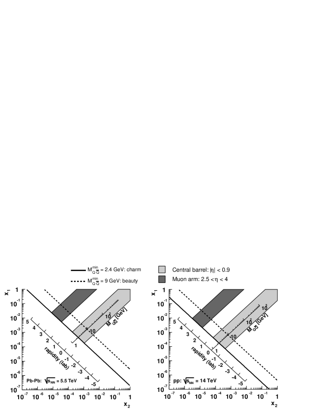
Figure 1: ALICE acceptance in the ($x_{1}$, $x_{2}$) plane for heavy flavours in Pb–Pb (left) and in pp (right). The figure is explained in detail in the text.

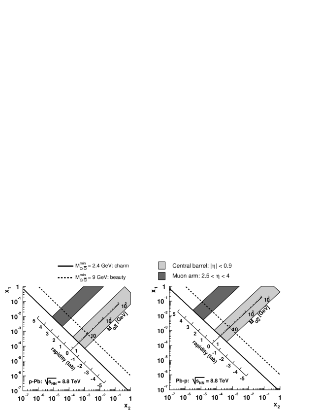
Figure 2: ALICE acceptance in the ($x_{1}$, $x_{2}$) plane for heavy flavours in p–Pb (left) and in Pb–p (right).

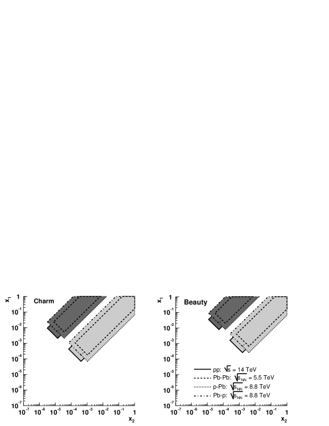
Figure 3: ALICE acceptance in the ($x_{1}$, $x_{2}$) plane for charm (left) and beauty (right) in pp, Pb–Pb, p–Pb and Pb–p.

Because of its lower mass, charm allows to probe lower $x$ values than beauty. The capability to measure charm and beauty particles in the forward rapidity region ($y\simeq 4$) would give access to $x$ regimes about 2 orders of magnitude lower, down to $x\sim 10^{-6}$.

In Fig. 3 we show the regions of the ($x_{1}$, $x_{2}$) plane covered for charm and beauty by the ALICE acceptance, in Pb–Pb at 5.5 TeV and in pp at 14 TeV. In this plane the points with constant invariant mass lie on hyperbolae ($x_{1}=M^{2}_{Q\overline{Q}}/(x_{2}\,s_{\scriptscriptstyle\rm NN})$), straight lines in the log-log scale: we show those corresponding to the production of $\mathrm{c\overline{c}}$ and $\mathrm{b\overline{b}}$ pairs at the threshold; the points with constant rapidity lie on straight lines ($x_{1}=x_{2}\exp(+2\,y_{Q\overline{Q}})$). The shadowed regions show the acceptance of the ALICE barrel, covering the pseudorapidity range $|\eta|<0.9$, and of the muon arm, $2.5<\eta<4$.

In the case of asymmetric collisions, e.g. p–Pb and Pb–p, we have a rapidity shift: the centre of mass moves with a longitudinal rapidity

$$y_{\rm c.m.}=\frac{1}{2}\ln\left(\frac{\rm Z_{1}A_{2}}{\rm Z_{2}A_{1}}\right),$$ (5)

obtained from equation (2) for $x_{1}=x_{2}$. The rapidity window covered by the experiment is consequently shifted by

$$\Delta y=y_{\rm lab.\leavevmode\nobreak\ system}-y_{\rm c.m.\leavevmode\nobreak\ system}=y_{\rm c.m.},$$ (6)

corresponding to $+0.47$ ($-0.47$) for p–Pb (Pb–p) collisions. Therefore, running with both p–Pb and Pb–p will allow to cover the largest interval in $x$. The c.m.s. energy in this case is 8.8 TeV. Figure 3 shows the acceptances for p–Pb and Pb–p, while in Fig. 3 the coverages in pp, Pb–Pb, p–Pb and Pb–p are compared for charm (left) and beauty (right).

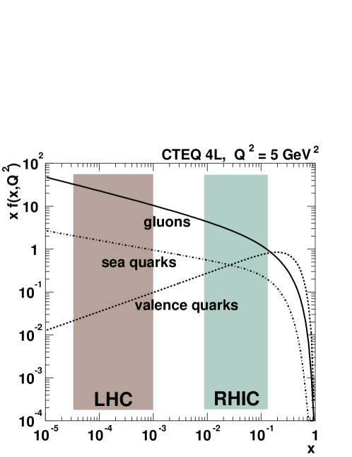
Figure 4: Parton distribution functions in the proton, in the CTEQ 4L parameterization, for $Q^{2}=5\leavevmode\nobreak\ \mbox{${\rm GeV}$}^{2}$.

These figures are meant to give a first idea of the regimes accessible with ALICE; the simple relations for the leading order case were used, the ALICE rapidity acceptance cuts were applied to the rapidity of the $Q\overline{Q}$ pair, and not to that of the particles which are actually detected. In addition, no minimum $p_{\rm t}$ cuts were accounted for: such cuts will increase the minimum accessible value of $M_{Q\overline{Q}}$, thus increasing also the minimum accessible $x$. These approximations, however, are not too drastic, since there is a very strong correlation in rapidity between the initial $Q\overline{Q}$ pair and the heavy flavour particles it produces and the minimum $p_{\rm t}$ cut will be quite low (lower than the mass of the hadron) for most of the channels studied with ALICE.

The parton distribution functions $x\,f(x,Q^{2})$ in the proton, in the CTEQ 4L parameterization [2], are shown in Fig. 4. $Q^{2}$ is the virtuality, or QCD scale (in the case of the leading order heavy flavour production considered in this paragraph, $Q^{2}=M^{2}_{Q\overline{Q}}=s\,x_{1}\,x_{2}$). In the figure the value $Q^{2}=5\leavevmode\nobreak\ \mbox{${\rm GeV}$}^{2}$, corresponding to $\mathrm{c\overline{c}}$ production at threshold, is used. The regions in $x$ covered, at central rapidities, at RHIC and LHC are indicated by the shaded areas.

2 Cross sections in nucleon–nucleon collisions

In this section we present the status of the cross section calculations in nucleon–nucleon collisions and their comparison with existing data up to a c.m.s. energy of $\simeq 65\leavevmode\nobreak\ \mbox{${\rm GeV}$}$. We then report the results for LHC energies. The extrapolation to heavy ion collisions is described in the next section.

Figure 5: Total charm production cross section from pp and pA measurements compared to NLO calculations [3] with MRS D-’ (solid), MRST HO (dashed) and MRST LO (dot-dashed) parton distributions.

Figure 6: Comparison with b quark production cross section integrated over $p_{\mathrm{t}}>p_{\mathrm{t}}^{\rm min}$ from (a) UA1 [4] and (b) CDF and D0 [5]. The NLO calculations are with MRS D-’ (solid) and GRV HO (dashed) parton distributions.

The existing data on total charm production cross section in pp and pA collisions up to ISR energies are compared in Fig. 6 with NLO calculations by R. Vogt [3]. In Fig. 6 a NLO calculation from Ref. [6] is compared to the data in $\mathrm{p\overline{p}}$ collisions from UA1, CDF and D0, for which the b quark production cross section integrated for $p_{\mathrm{t}}>p_{\mathrm{t}}^{\rm min}$ is given. These measurements are taken in the central rapidity region ($|y|<1.5$ for UA1, $|y|<1$ for CDF and D0). All the calculations have been performed using the following values for the heavy quark masses ($m_{\rm c}$, $m_{\rm b}$) and for the factorization and renormalization scales ($\mu_{F}$, $\mu_{R}$):

$$m_{\rm c}=1.2\leavevmode\nobreak\ \mbox{${\rm GeV}$}\,\,\,\,\,\,\,\,\,\,\,\,\,\,\,\,\,\,\,\,\,\,\,\,\,\,\,\,\,\,\,\,\,\,\,\,\,\,\,\mu_{F}=\mu_{R}=2\,\mu_{0}$$ (7)

for charm, and

$$m_{\rm b}=4.75\leavevmode\nobreak\ \mbox{${\rm GeV}$}\,\,\,\,\,\,\,\,\,\,\,\,\,\,\,\,\,\,\,\,\,\,\,\,\,\,\,\,\,\,\,\,\,\,\,\,\,\,\,\mu_{F}=\mu_{R}=\mu_{0}$$ (8)

for beauty; $\mu_{0}\equiv\sqrt{(p_{\rm t,Q}^{2}+p_{\rm t,\overline{Q}}^{2})/2+m_{Q}^{2}}$ is approximately equal to the transverse mass of the produced heavy quarks.

For both charm and beauty the theory describes the present data reasonably well.

The results for LHC energies ($\sqrt{s}=$ 5.5, 8.8 and 14 ${\rm TeV}$) are reported in Table 2. These values are obtained using the NLO pQCD calculation implemented in the program by M. Mangano, P. Nason and G. Ridolfi [7] (HVQMNR) and two sets of parton distribution functions, MRST HO [8] and CTEQ 5M1 [9], which include the small-$x$ HERA results. The difference due to the choice of the parton distribution functions is relatively small ($\sim 20$-$25\%$ at 5.5 ${\rm TeV}$, slightly lower at 14 ${\rm TeV}$). We chose to use as a baseline the average, also reported in the table, of the values obtained with these two sets of PDF.

Table 2: NLO calculation [7] for the total $\mathrm{c\overline{c}}$  and $\mathrm{b\overline{b}}$  cross sections in pp collisions at 5.5, 8.8 and 14 ${\rm TeV}$, using the MRST HO and CTEQ 5M1 parton distribution functions.

		$\sigma_{{\rm pp}}^{\scriptstyle{\rm c\overline{c}}}[{\rm mb}]$			$\sigma_{{\rm pp}}^{\scriptstyle{\rm b\overline{b}}}[{\rm mb}]$
$\sqrt{s}$	$5.5\leavevmode\nobreak\ \mbox{${\rm TeV}$}$	$8.8\leavevmode\nobreak\ \mbox{${\rm TeV}$}$	$14\leavevmode\nobreak\ \mbox{${\rm TeV}$}$	$5.5\leavevmode\nobreak\ \mbox{${\rm TeV}$}$	$8.8\leavevmode\nobreak\ \mbox{${\rm TeV}$}$	$14\leavevmode\nobreak\ \mbox{${\rm TeV}$}$
MRST HO	5.9	8.4	10.3	0.19	0.28	0.46
CTEQ 5M1	7.4	9.6	12.1	0.22	0.31	0.55
Average	6.6	9.0	11.2	0.21	0.30	0.51

Table 3: Charm and beauty total cross sections at NLO with different choices of the parameters $m_{\rm c}$ ($m_{\rm b}$), $\mu_{F}$ and $\mu_{R}$ [10]. In the last column the ratio of the cross sections at 5.5 TeV and at 14 TeV is reported.

	parameters	5.5 ${\rm TeV}$	14 ${\rm TeV}$	ratio 5.5 TeV/14 TeV
	$m_{\rm c}=1.5\leavevmode\nobreak\ \mbox{${\rm GeV}$}$
	$\mu_{R}=2\mu_{0}\,\,\,\,\,\,\mu_{F}=2\mu_{0}$	3.7	7.3	0.51
	$m_{\rm c}=1.2$ GeV
	$\mu_{R}=\mu_{0}\,\,\,\,\,\,\mu_{F}=2\mu_{0}$	9.2	16.7	0.55
	$m_{\rm c}=1.5$ GeV
	$\mu_{R}=\mu_{0}\,\,\,\,\,\,\mu_{F}=2\mu_{0}$	5.4	10.4	0.52
	$m_{\rm c}=1.8\leavevmode\nobreak\ \mbox{${\rm GeV}$}$
$\sigma_{{\rm pp}}^{\scriptstyle{\rm c\overline{c}}}[{\rm mb}]$	$\mu_{R}=\mu_{0}\,\,\,\,\,\,\mu_{F}=2\mu_{0}$	3.4	6.8	0.50
	$m_{\rm b}=4.5\leavevmode\nobreak\ \mbox{${\rm GeV}$}$
	$\mu_{R}=\mu_{0}\,\,\,\,\,\,\mu_{F}=\mu_{0}$	0.20	0.51	0.39
	$m_{\rm b}=4.75\leavevmode\nobreak\ \mbox{${\rm GeV}$}$
	$\mu_{R}=\mu_{0}\,\,\,\,\,\,\mu_{F}=\mu_{0}$	0.17	0.43	0.40
	$m_{\rm b}=5\leavevmode\nobreak\ \mbox{${\rm GeV}$}$
	$\mu_{R}=\mu_{0}\,\,\,\,\,\,\mu_{F}=\mu_{0}$	0.15	0.37	0.41
	$m_{\rm b}=4.75\leavevmode\nobreak\ \mbox{${\rm GeV}$}$
	$\mu_{R}=0.5\mu_{0}\,\,\,\,\,\,\mu_{F}=2\mu_{0}$	0.26	0.66	0.39
	$m_{\rm b}=4.75\leavevmode\nobreak\ \mbox{${\rm GeV}$}$
$\sigma_{{\rm pp}}^{\mbox{$\scriptstyle\mathrm{b\overline{b}}$}}[{\rm mb}]$	$\mu_{R}=2\mu_{0}\,\,\,\,\,\,\mu_{F}=0.5\mu_{0}$	0.088	0.20	0.44

The dependence on the PDF set represents only a part of the error on the theoretical estimate. An evaluation of the theoretical uncertainties was done by M. Mangano by varying the $m_{\rm c}$ ($m_{\rm b}$), $\mu_{F}$ and $\mu_{R}$ parameters and is reported in Table 3 [10]. This table shows that, at LHC energies, the theoretical uncertainties span a factor $\sim 2$-$3$ in the total production cross section of both charm and beauty quarks. In the last column of the table we report the ratio of the cross section at 5.5 TeV to that at 14 TeV. Despite the large spread of the absolute values, the ratio is much less dependent on the choice of the parameters; its value is $\simeq 0.52$ for charm and $\simeq 0.41$ for beauty. In Ref. [10] it is shown that also the ratios of the $p_{\mathrm{t}}$-differential cross sections are rather independent of the parameters choice. This indicates that pQCD can be used to compare the cross sections measured in Pb–Pb collisions at $\sqrt{s_{\scriptscriptstyle{{\rm NN}}}}=5.5\leavevmode\nobreak\ \mbox{${\rm TeV}$}$ to those measured in p–Pb at $\sqrt{s_{\scriptscriptstyle{{\rm NN}}}}=8.8\leavevmode\nobreak\ \mbox{${\rm TeV}$}$ and in pp at $\sqrt{s}=14\leavevmode\nobreak\ \mbox{${\rm TeV}$}$.

Yields in proton–proton collisions at $\sqrt{s}=14\leavevmode\nobreak\ \mbox{${\rm TeV}$}$

Using a proton–proton inelastic cross section $\sigma^{\rm inel}_{{\rm pp}}=70\leavevmode\nobreak\ {\rm mb}$ at 14 ${\rm TeV}$ [17] and the average heavy flavour cross sections in the last row of Table 2, we calculate the yields for the production of $Q\overline{Q}$ pairs as:

$$N_{{\rm pp}}^{\scriptstyle Q\overline{Q}}=\sigma_{{\rm pp}}^{\scriptstyle Q\overline{Q}}\bigg{/}\sigma^{\rm inel}_{{\rm pp}}.$$ (9)

We obtain 0.16 $\mathrm{c\overline{c}}$ pairs and 0.0072 $\mathrm{b\overline{b}}$ pairs per event.

3 Extrapolation to heavy ion collisions

In this section we derive the extrapolation of the cross sections and yields to central Pb–Pb collisions first, and then to p–Pb collisions. We also point out the different weight of the nuclear shadowing effect in the two cases, for charm and beauty production.

3.1 Nucleus–nucleus collisions

If no nuclear effects are taken into account, a nucleus–nucleus collision can be considered, for what concerns the hard cross section, as a superposition of independent nucleon–nucleon collisions. Thus, the cross section for hard processes in heavy ion collisions can be calculated using a simple geometrical extrapolation from pp collisions, i.e. assuming that the hard cross section scales from pp to nucleus–nucleus collisions proportionally to the number of inelastic nucleon–nucleon collisions (binary scaling).

Nuclear effects —such as nuclear shadowing, broadening of the parton intrinsic transverse momentum ($k_{\rm t}$) in the nucleon, in-medium parton energy loss, as well as possible enhancements due to thermal production in the medium— can modify this geometrical scaling from pp to nucleus–nucleus collisions. Such effects are, indeed, what we want to measure. We chose to include in the simulation only the nuclear shadowing and the broadening of the intrinsic $k_{\rm t}$, since they are well established effects. The first effect modifies the total hard cross section, while the broadening of the intrinsic $k_{\rm t}$ affects only the kinematic distributions of the produced heavy quarks. Nuclear shadowing can be accounted for by recalculating the hard cross section in elementary nucleon–nucleon collisions with nuclear-modified parton distribution functions and extrapolating to the nucleus–nucleus case.

The extrapolation, based on the Glauber model [11, 12], is derived for the collision of two generic nuclei with mass numbers A and B, and numerical examples are given for the specific case of Pb–Pb reactions at $\sqrt{s_{\scriptscriptstyle{{\rm NN}}}}=5.5\leavevmode\nobreak\ \mbox{${\rm TeV}$}$.

We are interested in the cross section for a sample of events in a given centrality range, defined by the trigger settings. The centrality selection can be assumed to correspond to a cut on the impact parameter $b$ of the collision: $0\leq b<b_{c}$. The sample of events defined by this cut contains a fraction of the total number of inelastic collisions, i.e. of the total inelastic cross section, given by

$$F(b_{c})=\int_{0}^{b_{c}}{\rm d}b\,\frac{{\rm d}\sigma^{\rm inel}_{\rm AB}}{{\rm d}b}\bigg{/}\int_{0}^{\infty}{\rm d}b\,\frac{{\rm d}\sigma^{\rm inel}_{\rm AB}}{{\rm d}b}.$$ (10)

The definition of the centrality in terms of fraction of the inelastic cross section is more appropriate, since the cross section is directly measured, while the impact parameter estimation depends on the model used to describe the geometry of the collision.

In the following, we consider two options for the centrality selection, corresponding to 5% and 10% of the total inelastic cross section. The values of $b_{c}$ that give these selections are $3.5\leavevmode\nobreak\ \mbox{${\rm fm}$}$ and $5\leavevmode\nobreak\ \mbox{${\rm fm}$}$, respectively.

The inelastic cross section corresponding to a given centrality selection is found integrating the interaction probability up to impact parameter $b_{c}$:

$$\sigma_{{\rm AB}}^{\mathrm{inel}}(b_{c})=\int_{0}^{b_{c}}{\rm d}b\,\frac{{\rm d}\sigma^{\rm inel}_{\rm AB}}{{\rm d}b}=2\pi\int_{0}^{b_{c}}b\,{\rm d}b\,\,\left\{1-[1-\sigma_{\scriptscriptstyle{{\rm NN}}}T_{{\rm AB}}(b)]^{{\rm AB}}\right\}$$ (11)

where the value $\sigma_{\scriptscriptstyle{{\rm NN}}}=60\leavevmode\nobreak\ {\rm mb}$ was used as the nucleon–nucleon inelastic cross section at 5.5 TeV [13], and the total thickness function $T_{{\rm AB}}$

$$T_{{\rm AB}}(b)=\int{\rm d}^{2}s\,T_{\rm A}(\vec{s})\,T_{\rm B}(\vec{s}-\vec{b})$$ (12)

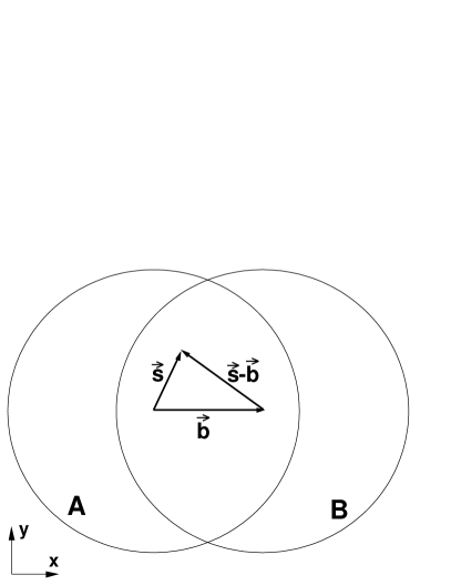
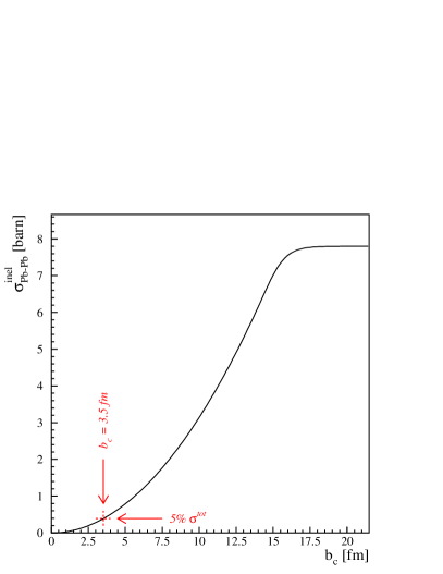
(vectors defined as in Fig. 7, left) is expressed in terms of the thickness function of the nucleus $T_{i}(\vec{s})=\int{\rm d}z\,\rho_{i}(z,\vec{s})$ for $i={\rm A,\,B}$, where $\rho_{i}$ is the Wood-Saxon nuclear density profile [14] —the thickness function is normalized to unity: $\int{\rm d^{2}}s\,T_{i}(\vec{s})=1$. In Fig. 7 (right) the inelastic cross section (11) is shown as a function of $b_{c}$.

Figure 7: Collision geometry in the plane transverse to the beam line (left). Inelastic Pb–Pb cross section as a function of the impact parameter cut $b<b_{c}$ (right); for clearness, here and in Fig. 8, only the value corresponding to 5% of the total inelastic cross section is explicitly indicated.

The average number of inelastic collisions for a given impact parameter $b$ is:

$$\sigma_{\scriptscriptstyle{{\rm NN}}}\cdot{\rm AB}\,\,T_{{\rm AB}}(b).$$ (13)

By replacing the inelastic nucleon–nucleon cross section $\sigma_{\scriptscriptstyle{{\rm NN}}}$ with the elementary cross section for a given hard process $\sigma_{\rm pp}^{\rm hard}$, we obtain the average number of inelastic collisions that yield the considered hard process:

$$\sigma_{\rm pp}^{\rm hard}\cdot{\rm AB}\,\,T_{{\rm AB}}(b),$$ (14)

and the cross section for hard processes for $0\leq b<b_{c}$:

$$\sigma_{{\rm AB}}^{\mathrm{hard}}(b_{c})=\sigma_{{\rm pp}}^{\mathrm{hard}}\cdot 2\pi\,\int_{0}^{b_{c}}b\,{\rm d}b\,\,{\rm AB}\,\,T_{{\rm AB}}(b).$$ (15)

For minimum-bias collisions ($b_{c}=+\infty$), we have:

$$\sigma_{{\rm AB}}^{\mathrm{hard}}=\sigma_{{\rm pp}}^{\mathrm{hard}}\,{\rm AB}.$$ (16)

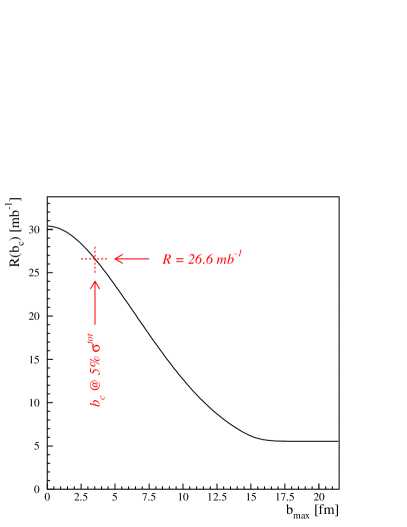
Figure 8: Cross section for a hard process in Pb–Pb collisions relative to the one in nucleon–nucleon collisions as a function of the impact parameter cut $b<b_{c}$ (left). Yield of the hard process in Pb–Pb collisions relative to the cross section in nucleon–nucleon collisions as a function of the impact parameter cut $b<b_{c}$ (right).

The ratio of the hard cross section in nucleus–nucleus collisions, with a centrality cut $b<b_{c}$, relative to the cross section in nucleon–nucleon interactions is (see Fig. 8, left):

$$f^{\mathrm{hard}}(b_{c})=\frac{\sigma_{{\rm AB}}^{\mathrm{hard}}(b_{c})}{\sigma_{{\rm pp}}^{\mathrm{hard}}}=2\pi\int_{0}^{b_{c}}b\,{\rm d}b\,\,{\rm AB}\,\,T_{{\rm AB}}(b).$$ (17)

The number (yield) of hard processes per triggered event is:

$$N_{{\rm AB}}^{\mathrm{hard}}(b_{c})=\frac{\sigma_{{\rm AB}}^{\mathrm{hard}}(b_{c})}{\sigma_{{\rm AB}}^{\mathrm{inel}}(b_{c})}=\mathcal{R}(b_{c})\cdot\sigma_{{\rm pp}}^{\mathrm{hard}}$$ (18)

where (Fig. 8, right)

$$\mathcal{R}(b_{c})=\frac{\int_{0}^{b_{c}}b\,{\rm d}b\,\,{\rm AB}\,\,T_{{\rm AB}}(b)}{\int_{0}^{b_{c}}b\,{\rm d}b\,\,\left\{1-[1-\sigma_{\scriptstyle{{\rm NN}}}T_{{\rm AB}}(b)]^{{\rm AB}}\right\}}.$$ (19)

For a 5% (10%) centrality cut in Pb–Pb collisions, the yield $N_{\rm AB}^{\rm hard}$ is obtained by multiplying the elementary cross sections by $26.6\leavevmode\nobreak\ (23.7)\leavevmode\nobreak\ {\rm mb}^{-1}$.

Cross sections and yields in Pb–Pb collisions at $\sqrt{s_{\scriptscriptstyle{{\rm NN}}}}=5.5\leavevmode\nobreak\ \mbox{${\rm TeV}$}$

We used the EKS98 parameterization [15] of nuclear shadowing, which corresponds to a modification of the parton distribution functions of the nucleon in the nucleus, $f_{i}^{\rm A}(x,Q^{2})$, with respect to the ones of the free nucleon, $f_{i}^{\rm N}(x,Q^{2})$:

$$R_{i}^{\rm A}(x,Q^{2})=\frac{f_{i}^{\rm A}(x,Q^{2})}{f_{i}^{\rm N}(x,Q^{2})}$$ (20)

where the parton distribution functions are given as a function of the momentum fraction $x$ carried by the parton inside the nucleon and of the QCD scale $Q^{2}$ and $i=q_{\rm v},\,q_{\rm sea},\,g$ for valence quarks, sea quarks and gluons.

Figure 9: Shadowing factor $R$ for gluons in a ²⁰⁸Pb nucleus as a function of $x$ for three values of $Q^{2}$.

The shadowing factor $R_{g}^{\rm Pb}$ for gluons in a ²⁰⁸Pb nucleus is shown in Fig. 9. The centrality dependence of the shadowing is weak for collisions in the considered centrality range (up to 10% of $\sigma^{\rm inel}$) [16] and it is neglected here.

The reduction of the cross section due to shadowing amounts to about 35% for $\mathrm{c\overline{c}}$ pairs, while it amounts only to about 15% for $\mathrm{b\overline{b}}$ pairs, since, as seen in Section 1, beauty production corresponds to larger values of $x$, that are less affected by the shadowing suppression. In Section 4 we will show how nuclear shadowing modifies the heavy quark kinematical distributions.

Table 4 reports the charm and beauty total cross sections and yields in pp (with and without shadowing) and Pb–Pb collisions at $\sqrt{s_{\scriptscriptstyle{{\rm NN}}}}=5.5\leavevmode\nobreak\ \mbox{${\rm TeV}$}$, as calculated with the HVQMNR program. The values shown correspond to the average of the results obtained with MRST HO and CTEQ 5M1 parton distribution functions. For the Pb–Pb case we report the two centrality options: 5% and 10% of the total inelastic cross section. We have $\sigma^{\scriptstyle Q\overline{Q}}_{\rm Pb-Pb}(5\%\leavevmode\nobreak\ \sigma^{\rm inel})/\sigma^{\scriptstyle Q\overline{Q}}_{\rm Pb-Pb}(10\%\leavevmode\nobreak\ \sigma^{\rm inel})\simeq 1.12$.

Table 4: Total cross sections and yields for charm and beauty production in pp and Pb–Pb collisions at $\sqrt{s_{\scriptscriptstyle{{\rm NN}}}}=5.5\leavevmode\nobreak\ \mbox{${\rm TeV}$}$. The effect of shadowing is shown as the ratio $C_{\rm shad}$ of the cross section calculated with and without the modification of the parton distribution functions. For the Pb–Pb case we report the two centrality options: 5% and 10% of the total inelastic cross section.

		Charm	Beauty
	w/o shadowing	6.64	0.21
$\sigma^{\scriptstyle Q\overline{Q}}_{{\rm pp}}\,[{\rm mb}]$	w/ shadowing	4.32	0.18
$C_{\rm shad}$		0.65	0.84
	$5\%\leavevmode\nobreak\ \sigma^{\rm inel}$	45.0	1.79
$\sigma^{\scriptstyle Q\overline{Q}}_{\rm Pb-Pb}[{\rm b}]$	$10\%\leavevmode\nobreak\ \sigma^{\rm inel}$	40.1	1.59
	$5\%\leavevmode\nobreak\ \sigma^{\rm inel}$	115	4.56
$N^{\scriptstyle Q\overline{Q}}_{\rm Pb-Pb}$	$10\%\leavevmode\nobreak\ \sigma^{\rm inel}$	102	4.06

3.2 Proton–nucleus collisions

For the extrapolation to proton–nucleus collisions we use the geometrical Glauber-based method already described for the case of nucleus–nucleus collisions. If we consider minimum-bias collisions (with no centrality selection), and we use $\rm B=1$ and $T_{\rm B}(\vec{s})=\delta(\vec{s})$ for the proton, the total cross section for hard processes (15) becomes:

$$\sigma_{{\rm pA}}^{\mathrm{hard}}=\sigma_{{\rm pp}}^{\mathrm{hard}}\cdot 2\pi\,\int_{0}^{\infty}b\,{\rm d}b\,\,{\rm A}\,\,T_{{\rm A}}(b)={\rm A}\,\sigma_{{\rm pp}}^{\mathrm{hard}}.$$ (21)

The number of hard processes per minimum-bias pA collision is:

$$N^{\rm hard}_{\rm pA}={\rm A}\,\sigma^{\rm hard}_{\rm pp}\bigg{/}\sigma^{\rm inel}_{\rm pA}.$$ (22)

Cross sections and yields in p–Pb collisions at $\sqrt{s_{\scriptscriptstyle{{\rm NN}}}}=8.8\leavevmode\nobreak\ \mbox{${\rm TeV}$}$

Using $\rm A=208$ and $\sigma_{\rm p-Pb}^{\rm inel}=1.9$ barn [17], the yield of $Q\overline{Q}$ pairs per minimum-bias collision is:

$$N^{\scriptstyle Q\overline{Q}}_{\rm p-Pb}=\sigma^{\scriptstyle Q\overline{Q}}_{\rm pp}\cdot 0.109\leavevmode\nobreak\ {\rm mb^{-1}}.$$ (23)

As for the Pb–Pb case, the effect of nuclear shadowing was accounted for by using the EKS98 parameterization [15]. Clearly, the effect is lower for p–Pb, since one of the colliding nuclei is a proton: the reduction of the cross sections due to nuclear shadowing is 20% for charm and 10% for beauty.

The cross sections and yields for charm and beauty production in pp (with and without shadowing) and minimum-bias p–Pb collisions at $\sqrt{s_{\scriptscriptstyle{{\rm NN}}}}=8.8\leavevmode\nobreak\ \mbox{${\rm TeV}$}$ are reported in Table 5. The values shown correspond to the average of the results obtained with MRST HO and CTEQ 5M1 parton distribution functions.

A summary of the production yields and of the average magnitude of nuclear shadowing in the three considered colliding systems is presented in Table 6.

Table 5: Total cross sections and yields for charm and beauty production in pp and p–Pb collisions at $\sqrt{s_{\scriptscriptstyle{{\rm NN}}}}=8.8\leavevmode\nobreak\ \mbox{${\rm TeV}$}$. The effect of shadowing is shown as the ratio $C_{\rm shad}$ of the cross section calculated with and without the modification of the parton distribution functions.

		Charm	Beauty
	w/o shadowing	9.00	0.30
$\sigma^{\scriptstyle Q\overline{Q}}_{{\rm pp}}\,[{\rm mb}]$	w/ shadowing	7.16	0.27
$C_{\rm shad}$		0.80	0.90
$\sigma^{\scriptstyle Q\overline{Q}}_{\rm p-Pb}[{\rm b}]$		1.49	0.056
$N^{\scriptstyle Q\overline{Q}}_{\rm p-Pb}$		0.78	0.029

Table 6: Summary table of the production yields and of the average magnitude of nuclear shadowing in pp, p–Pb and Pb–Pb.

		Charm			Beauty
system	pp	p–Pb	Pb–Pb	pp	p–Pb	Pb–Pb
centrality	min.-bias	min.-bias	centr. (5%)	min.-bias	min.-bias	centr. (5%)
$\sqrt{s_{\scriptscriptstyle{{\rm NN}}}}$	$14\leavevmode\nobreak\ \mbox{${\rm TeV}$}$	$8.8\leavevmode\nobreak\ \mbox{${\rm TeV}$}$	$5.5\leavevmode\nobreak\ \mbox{${\rm TeV}$}$	$14\leavevmode\nobreak\ \mbox{${\rm TeV}$}$	$8.8\leavevmode\nobreak\ \mbox{${\rm TeV}$}$	$5.5\leavevmode\nobreak\ \mbox{${\rm TeV}$}$
$N^{\scriptstyle Q\overline{Q}}$/ev	0.16	0.78	115	0.0072	0.029	4.56
$C_{\rm shad}$	1	0.80	0.65	1	0.90	0.84

4 Heavy quark kinematical distributions

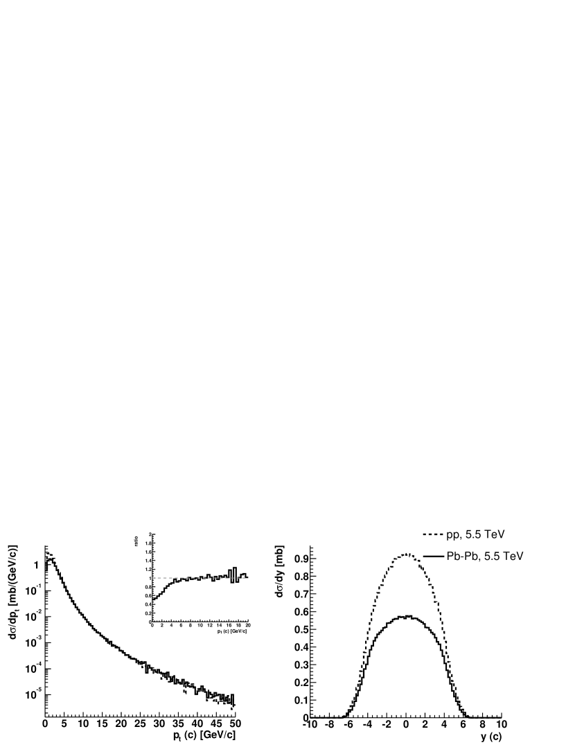
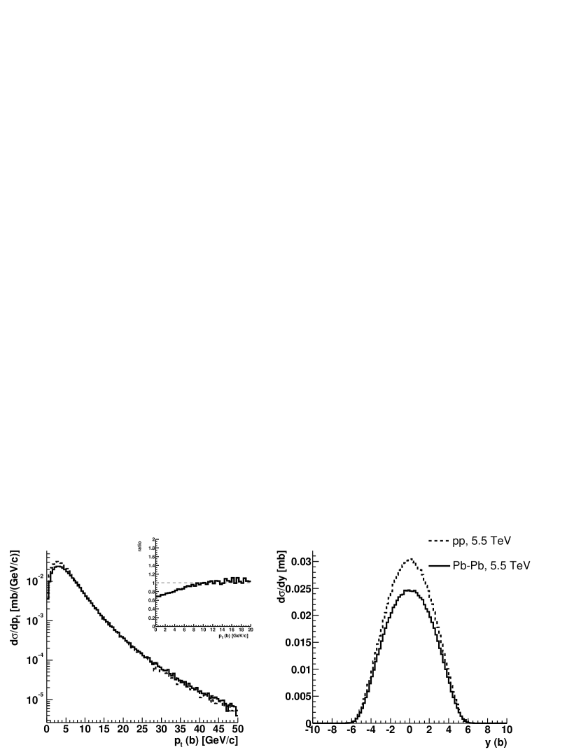
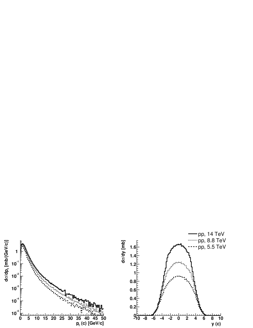
Figures 10 and 11 present the transverse momentum and rapidity distributions, obtained using the NLO pQCD program HVQMNR, for c and b quarks, respectively. The distributions for Pb–Pb and p–Pb are normalized to the cross section per nucleon–nucleon collision.

Figure 10: Inclusive c quark $p_{\mathrm{t}}$ and rapidity distributions obtained from the HVQMNR program. The distributions for Pb–Pb and p–Pb are normalized to the cross sections per nucleon–nucleon collision and they include the effects of nuclear shadowing and intrinsic $k_{\rm t}$ broadening.

Figure 11: Inclusive b quark $p_{\mathrm{t}}$ and rapidity distributions obtained from the HVQMNR program. The distributions for Pb–Pb and p–Pb are normalized to the cross sections per nucleon–nucleon collision and they include the effects of nuclear shadowing and intrinsic $k_{\rm t}$ broadening.

We used the CTEQ 4M [2] set of PDF. We verified that the results given by this set lie in between the ones obtained with the more recent CTEQ 5 and MRST sets for all the relevant kinematical quantities [10]. For the other parameters to values specified in Section 2 were used: $m_{\rm c}=1.2\leavevmode\nobreak\ \mbox{${\rm GeV}$}$, $\mu_{R}=\mu_{F}=2\,\mu_{0}$ for charm and $m_{\rm b}=4.75\leavevmode\nobreak\ \mbox{${\rm GeV}$}$, $\mu_{R}=\mu_{F}=\mu_{0}$ for beauty. Nuclear shadowing is included via the EKS98 parameterization [15]. The parton intrinsic $k_{\rm t}$ is sampled from a Gaussian distribution with mean 0 and $\sigma$ ($=\sqrt{\left\langle k_{\rm t}^{2}\right\rangle}$) equal to 1, 1.16, $1.30\leavevmode\nobreak\ \mbox{${\rm GeV}$}/c$ for charm production in pp, p–Pb and Pb–Pb, respectively, and equal to 1, 1.60, $2.04\leavevmode\nobreak\ \mbox{${\rm GeV}$}/c$ for beauty production in pp, p–Pb and Pb–Pb, respectively. These values are taken from Ref. [3]. The same parameters are used also in the calculations shown in the next section.

In the case of p–Pb events the rapidity distribution in the centre-of-mass frame is plotted; the rapidity distribution in the laboratory frame would be shifted by $\Delta y=0.47$.

We notice that the $p_{\mathrm{t}}$ distributions for pp collisions at 5.5, 8.8 and 14 TeV (top-left panel) have essentially the same shape.

The comparison of the $p_{\mathrm{t}}$ distributions for pp and Pb–Pb (and for pp and p–Pb) at the same centre-of-mass energy shows that nuclear shadowing affects heavy quark production only for relatively low transverse momenta ($p_{\mathrm{t}}<5$-$6\leavevmode\nobreak\ \mbox{${\rm GeV}$}/c$ with EKS98), where the $\mathrm{Q\overline{Q}}$ pairs are produced by low-$x$ gluons. This is clearly seen in the ratios of the distributions, reported in the insets. The value for the upper limit, $\approx 5\leavevmode\nobreak\ \mbox{${\rm GeV}$}/c$, of the $p_{\mathrm{t}}$-region affected by the shadowing in Pb–Pb collisions can be cross-checked with the following simple estimate: for the back-to-back production of a $\mathrm{c\overline{c}}$ pair at central rapidity, with transverse momenta $p_{\mathrm{t}}^{\rm c}=p_{\mathrm{t}}^{\rm\overline{c}}=5\leavevmode\nobreak\ \mbox{${\rm GeV}$}/c$, we have $Q\simeq 2\,p_{\mathrm{t}}=10\leavevmode\nobreak\ \mbox{${\rm GeV}$}$ and $x\simeq Q/\sqrt{s_{\scriptscriptstyle{{\rm NN}}}}=10/5500\simeq 2\cdot 10^{-3}$; for these values of $x$ and $Q$, the EKS98 parameterization gives $R^{\rm Pb}_{g}$ (defined in Eq. (20)) $\simeq 90\%$. This suppression is already quite small and it is partially compensated by the $k_{\rm t}$ broadening.

A relevant feature of $\mathrm{Q\overline{Q}}$ production in p–Pb collisions is a depletion in the forward region (where the proton goes) of the rapidity distributions. This effect is due to the shadowing which is biased toward forward rapidities, where the smallest $x$ values in the Pb nucleus are probed.

5 Heavy quark production in Monte Carlo event generators

The program used for the NLO calculations reported in the previous sections is not well suited to be included in a simulation, since it is not an event generator and it does not provide parton kinematics, but only inclusive distribution. On the other hand, widely used event generators, like PYTHIA [18] and HERWIG [19], are exact only at leading order, when only the pair production processes, $q\overline{q}\to Q\overline{Q}$ and $gg\to Q\overline{Q}$ (see Fig. 12), are included. Higher-order contributions are included in these generators in the parton shower approach (see e.g. Ref. [20]). This model is not exact at next-to-leading order, but it reproduces some aspects of the multiple-parton-emission phenomenon. In the following we will concentrate on the PYTHIA event generator; the version we have used is PYTHIA 6.150. We have also investigated heavy quark production in HERWIG, observing an incorrect behaviour in the final kinematical distributions of both c and b quarks. We, therefore, concluded that HERWIG is not suitable for heavy quark simulations at LHC energies. More details can be found in Ref. [10].

Figure 12: Some of the PYTHIA processes defined as pair creation, flavour excitation and gluon splitting. The thick lines correspond to the hard process, the thin ones to the initial- or final-state parton shower.

Figure 13: Comparison between PYTHIA results (solid histogram) for the LO process $gg\to c\overline{c}$, without parton shower, and corresponding HVQMNR prediction (dashed histogram). The centre of mass energy is $\sqrt{s}=5.5\leavevmode\nobreak\ \mbox{${\rm TeV}$}$.

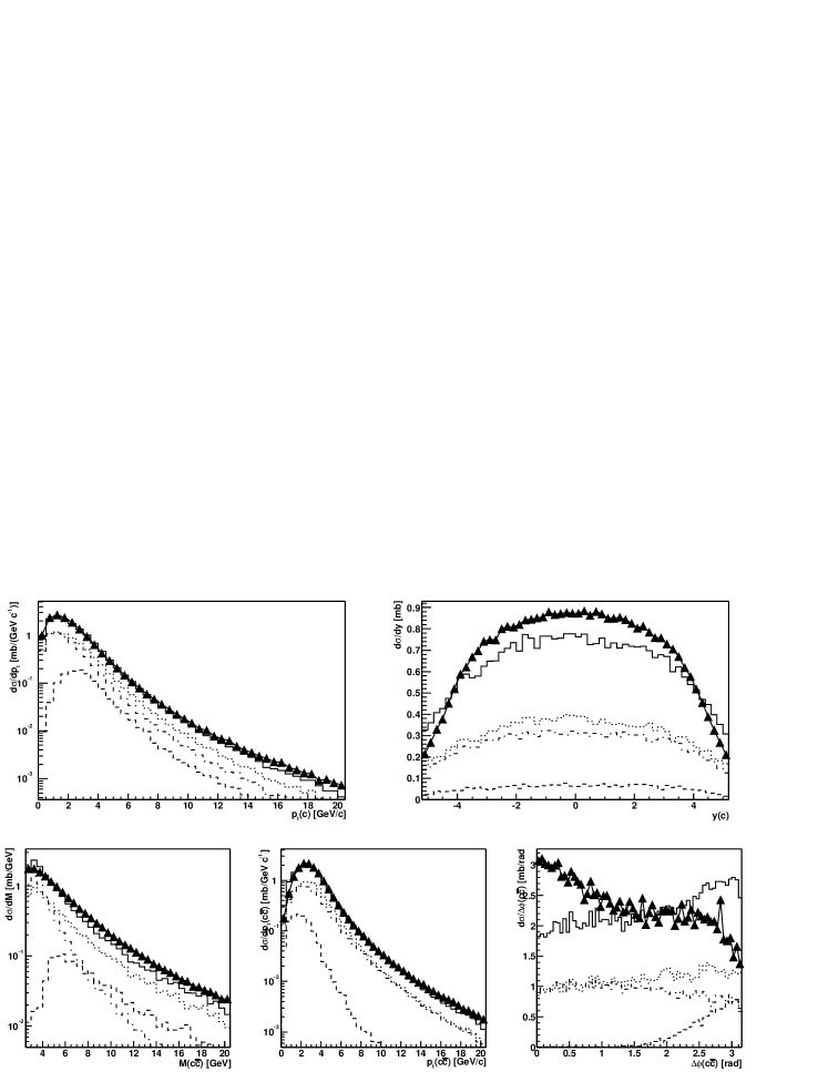
In PYTHIA, the processes giving rise to contributions above leading order, like (see Fig. 12) flavour excitation, $qQ\rightarrow qQ$ and $gQ\rightarrow gQ$, and gluon splitting, $g\rightarrow Q\overline{Q}$, are calculated using a massless matrix element. As a consequence the cross sections for these processes diverge as $p_{\mathrm{t}}^{\rm hard}$ vanishes. These divergences are regularized by putting a lower cut-off on $p_{\mathrm{t}}^{\rm hard}$. The value of the minimum $p_{\mathrm{t}}^{\rm hard}$ cut has a large influence on the heavy flavour cross section at low $p_{\mathrm{t}}$, a region of prime interest for ALICE physics and covered by the ALICE acceptance. Our approach was, therefore, to tune the PYTHIA parameters in order to reproduce as well as possible the NLO predictions (HVQMNR). We used PYTHIA with the option MSEL=1, that allows to switch on one by one the different processes (see the Appendix for more details). The main parameter we tuned is the lower $p_{\mathrm{t}}^{\rm hard}$ limit. In this procedure we compared the following distributions of the bare quarks:

• inclusive $p_{\mathrm{t}}$ and rapidity distributions of the quark (antiquark);

• mass of the pair: $M_{Q\overline{Q}}=\sqrt{(E_{Q}+E_{\overline{Q}})^{2}-(\vec{p}_{Q}+\vec{p}_{\overline{Q}})^{2}}$, where $E_{Q}=\sqrt{m_{Q}^{2}+p_{Q}^{2}}$ is the quark energy;

• $p_{\mathrm{t}}$ of the pair, defined as the projection on the plane normal to the beam axis of the $Q\overline{Q}$ total momentum;

• angle $\Delta\phi$ between the quark and the antiquark in the plane normal to the beam axis.

In the simulations for Pb–Pb collisions at $\sqrt{s_{\scriptscriptstyle{{\rm NN}}}}=5.5\leavevmode\nobreak\ \mbox{${\rm TeV}$}$ the parton distribution functions used are the CTEQ 4, modified for nuclear shadowing using the EKS98 [15] parameterization.

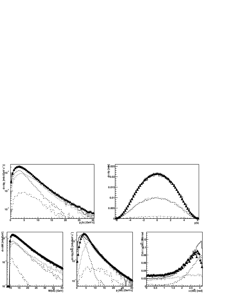
Figure 14: Comparison between charm production in Pb–Pb collisions at $\sqrt{s_{\scriptscriptstyle{{\rm NN}}}}=5.5\leavevmode\nobreak\ \mbox{${\rm TeV}$}$ in the HVQMNR NLO calculation and in PYTHIA with parameters tuned as described in the text. The triangles show the NLO calculation, the solid histogram corresponds to the PYTHIA total production. The individual PYTHIA contributions are pair production (dashed), flavour excitation (dotted) and gluon splitting (dot-dashed).

Figure 15: Equivalent of Fig. 15 for beauty production.

Figure 16: Comparison between charm production in pp collisions at $\sqrt{s}=14\leavevmode\nobreak\ \mbox{${\rm TeV}$}$ in the HVQMNR NLO calculation and in PYTHIA with parameters tuned as described in the text. The triangles show the NLO calculation, the solid histogram corresponds to the PYTHIA total production. The individual PYTHIA contributions are pair production (dashed), flavour excitation (dotted) and gluon splitting (dot-dashed).

Figure 17: Equivalent of Fig. 17 for beauty production.

Before presenting the results of the tuning of PYTHIA to reproduce the pQCD results at NLO, we show that, with the same input parameters, PYTHIA and the pQCD calculation in HVQMNR give exactly the same kinematical distributions for the LO process $gg\to Q\overline{Q}$. The comparison is reported in Fig. 13 for $\mathrm{c\overline{c}}$ production in pp collisions at $\sqrt{s}=5.5\leavevmode\nobreak\ \mbox{${\rm TeV}$}$; the normalization is set to the value of the cross section obtained for proton–proton without shadowing (first row of Table 4) and the PYTHIA results are scaled to this number.

The results of the tuning to pQCD at NLO are shown in Figs. 15 and 15, where the distributions from PYTHIA and the NLO calculation are compared. In this case the overall normalization is set to the value of the cross sections obtained for proton–proton with shadowing (second row of Table 4). Despite the fundamental differences between the two models, the agreement is relatively good. However, significant discrepancies are present, especially in the $\Delta\phi$ distribution for $\mathrm{c\overline{c}}$ pairs.

A similar tuning of the PYTHIA event generator was done also for the production of $\mathrm{c\overline{c}}$ and $\mathrm{b\overline{b}}$ pairs in pp collisions at $\sqrt{s}=14\leavevmode\nobreak\ \mbox{${\rm TeV}$}$. The same set of parton distribution functions (CTEQ 4) was used, without the modification for nuclear shadowing. Results are shown in Figs. 17 and 17. The largest difference with the results obtained for the Pb–Pb case is a worse description of the rapidity distribution of charm quarks. This is due to a feature of the parameterizations of the parton distribution functions: most of them, including CTEQ 4, are valid only down to $x=10^{-5}$; below this value the behaviour depends on the implementation of the specific parameterization but has no physical meaning (e.g. for the CTEQ 4 the gluon density $g(x)$ is kept constant at $g(10^{-5})$). The rapidity range in which the evolution of the parton distribution functions is reliable depends on the c.m.s. energy; for charm production at $\sqrt{s}=5.5\leavevmode\nobreak\ \mbox{${\rm TeV}$}$ (14 ${\rm TeV}$) this range is found to be $|y|<4.3$ ($|y|<3.4$), using equation (4) with $x_{1}>10^{-5}$ and $x_{2}>10^{-5}$. This feature is not present in the latest CTEQ set of PDF, CTEQ 6 [21], which is evolved down to $x=10^{-6}$.

The values of the PYTHIA parameters obtained from the tuning are reported in the Appendix.

6 Hadron yields and distributions

For the hadronization of heavy quarks we use the default Lund string fragmentation model [20] included in PYTHIA (JETSET package). The total yield and the rapidity density d$N$/d$y$ in the central region for hadrons with open charm and beauty in Pb–Pb at 5.5 ${\rm TeV}$ ($5\%\leavevmode\nobreak\ \sigma^{\rm tot}$ centrality selection), pp at 14 ${\rm TeV}$ and p–Pb at $8.8\leavevmode\nobreak\ \mbox{${\rm TeV}$}$ are summarized in Tables 9, 9 and 9, respectively. The rapidity densities are calculated in $-1<y_{\rm lab}<1$, corresponding to $-1.47<y_{\rm c.m.s.}<0.53$ for p–Pb and $-0.53<y_{\rm c.m.s.}<1.47$ for Pb–p. No dependence of the relative hadron abundances on the centre-of-mass energy is observed.

Table 7: Total yield and average rapidity density for $|y|<1$ for hadrons with charm and beauty in Pb–Pb collisions at $\sqrt{s_{\scriptscriptstyle{{\rm NN}}}}=5.5\leavevmode\nobreak\ \mbox{${\rm TeV}$}$. The values reported correspond to a centrality selection of $5\%\leavevmode\nobreak\ \sigma^{\rm tot}$.

Particle	Yield	$\langle$d$N$/d$y\rangle_{|y|<1}$	Particle	Yield	$\langle$d$N$/d$y\rangle_{|y|<1}$
${\rm D^{0}}$	68.9	6.87	${\rm B^{0}}$	1.86	0.273
${\rm\overline{D}^{0}}$	71.9	6.83	${\rm\overline{B}^{0}}$	1.79	0.262
${\rm D^{+}}$	22.4	2.12	${\rm B^{+}}$	1.82	0.251
${\rm D^{-}}$	22.2	2.00	${\rm B^{-}}$	1.83	0.270
${\rm D_{s}^{+}}$	14.1	1.30	${\rm B_{s}^{0}}$	0.53	0.077
${\rm D_{s}^{-}}$	12.7	1.22	${\rm\overline{B}_{s}^{0}}$	0.53	0.082
${\rm\Lambda_{c}^{+}}$	9.7	1.18	${\rm\Lambda_{b}^{0}}$	0.36	0.050
${\rm\overline{\Lambda_{c}}^{-}}$	8.2	0.85	${\rm\overline{\Lambda_{b}}^{0}}$	0.31	0.047

Table 8: Total yield and average rapidity density for $|y|<1$ for hadrons with charm and beauty in pp collisions at $\sqrt{s}=14\leavevmode\nobreak\ \mbox{${\rm TeV}$}$.

Particle	Yield	$\langle$d$N$/d$y\rangle_{|y|<1}$	Particle	Yield	$\langle$d$N$/d$y\rangle_{|y|<1}$
${\rm D^{0}}$	0.0938	0.0098	${\rm B^{0}}$	0.00294	0.00043
${\rm\overline{D}^{0}}$	0.0970	0.0098	${\rm\overline{B}^{0}}$	0.00283	0.00041
${\rm D^{+}}$	0.0297	0.0029	${\rm B^{+}}$	0.00287	0.00040
${\rm D^{-}}$	0.0290	0.0029	${\rm B^{-}}$	0.00289	0.00043
${\rm D_{s}^{+}}$	0.0186	0.0018	${\rm B_{s}^{0}}$	0.00084	0.00012
${\rm D_{s}^{-}}$	0.0176	0.0020	${\rm\overline{B}_{s}^{0}}$	0.00084	0.00013
${\rm\Lambda_{c}^{+}}$	0.0113	0.0013	${\rm\Lambda_{b}^{0}}$	0.00057	0.00008
${\rm\overline{\Lambda_{c}}^{-}}$	0.0110	0.0013	${\rm\overline{\Lambda_{b}}^{0}}$	0.00049	0.00008

Table 9: Total yield and average rapidity density for $|y_{\rm lab}|<1$ for hadrons with charm and beauty in p–Pb collisions at $\sqrt{s_{\scriptscriptstyle{{\rm NN}}}}=8.8\leavevmode\nobreak\ \mbox{${\rm TeV}$}$.

Particle	Yield	$\langle$d$N$/d$y\rangle_{|y_{\rm lab}|<1}$	Particle	Yield	$\langle$d$N$/d$y\rangle_{|y_{\rm lab}|<1}$
${\rm D^{0}+\overline{D}^{0}}$	0.926	0.096	${\rm B^{0}+\overline{B}^{0}}$	0.0221	0.0030
${\rm D^{+}+D^{-}}$	0.293	0.030	${\rm B^{+}+B^{-}}$	0.0221	0.0030
${\rm D_{s}^{+}+D_{s}^{-}}$	0.176	0.018	${\rm B_{s}^{0}+\overline{B}_{s}^{0}}$	0.0064	0.0009
${\rm\Lambda_{c}^{+}+\overline{\Lambda_{c}}^{-}}$	0.118	0.012	${\rm\Lambda_{b}^{0}+\overline{\Lambda_{b}}^{0}}$	0.0041	0.0005

It is interesting to notice the large ratio of the neutral-to-charged D meson yields: $N({\rm D^{0}})/N({\rm D^{+}})\simeq 3.1$. In PYTHIA, charm quarks are assumed to fragment to D (spin singlets: $J=0$) and D^∗ (spin triplets: $J=1$) mesons according to the number of available spin states; therefore, $N({\rm D^{0}}):N({\rm D^{+}}):N({\rm D^{*0}}):N({\rm D^{*+}})=1:1:3:3$. Then, the resonances D^∗ are decayed to D mesons according to the branching ratios. The difference between neutral and charged D mesons arises here: due to the slightly larger ($\approx 4\leavevmode\nobreak\ \mbox{${\rm MeV}$}$) mass of the D⁺, the D^∗+ decays preferably to $\mathrm{D^{0}}$ and the D^∗0 decays exclusively to $\mathrm{D^{0}}$. We have [13]:

$$\begin{array}[]{rcl}\displaystyle\frac{N({\rm D^{0}})}{N({\rm D^{+}})}&=&\displaystyle\frac{N({\rm D^{0}_{primary}})+N({\rm D^{*+}})\times BR({\rm D^{*+}\to D^{0}})+N({\rm D^{*0}})\times BR({\rm D^{*0}\to D^{0}})}{N({\rm D^{+}_{primary}})+N({\rm D^{*+}})\times BR({\rm D^{*+}\to D^{+}})+N({\rm D^{*0}})\times BR({\rm D^{*0}\to D^{+}})}\\ &=&\displaystyle\frac{1+3\times 0.68+3\times 1}{1+3\times 0.32+3\times 0}\\ &=&3.08.\end{array}$$ (24)

We chose to use the relative abundances given by PYTHIA, although, experimentally, the fraction $\mbox{$\mathrm{D^{0}}$}/{\rm D^{+}}$ was found to be lower than 3. The value measured in $e^{+}e^{-}$ collisions at LEP by the ALEPH Collaboration is $\approx 2.4$ [22]. This would reduce by about 6% the expected yield for the $\mathrm{D^{0}}$ mesons.

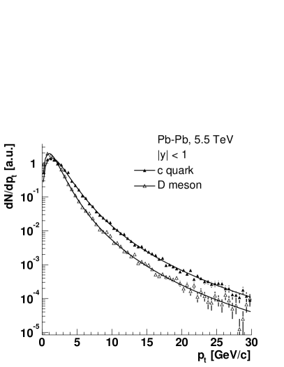
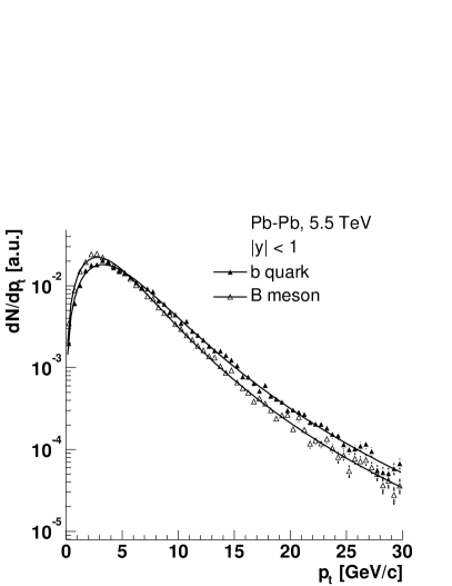
Figure 18: Transverse momentum distributions at mid-rapidity for heavy quarks and mesons in Pb–Pb at 5.5 TeV. The distributions are normalized to the same integral in order to compare their shapes.

Figure 18 presents the transverse momentum distributions at mid-rapidity ($|y|<1$) for c quarks and D mesons (left panel) and for b quarks and B mesons (right panel), in Pb–Pb at 5.5 ${\rm TeV}$. For $p_{\mathrm{t}}>0$ and $|y|<1$, we have, on average, $p_{\mathrm{t}}^{\rm D}\simeq 0.75\,p_{\mathrm{t}}^{\rm c}$ and $p_{\mathrm{t}}^{\rm B}\simeq 0.85\,p_{\mathrm{t}}^{\rm b}$. The shape of the transverse momentum distributions for D and B mesons was fitted to the following expression:

$$\frac{1}{p_{\mathrm{t}}}\frac{{\rm d}N}{{\rm d}p_{\mathrm{t}}}\propto\left[1+\left(\frac{p_{\mathrm{t}}}{p_{\mathrm{t}}^{0}}\right)^{2}\right]^{-n}.$$ (25)

The $p_{\mathrm{t}}$ distributions were studied also for pp at 14 TeV and for p–Pb at 8.8 TeV. The results of the fits are reported in Table 10, together with the average $p_{\mathrm{t}}$ of D and B mesons in the different conditions. The average $p_{\mathrm{t}}$ does not depend strongly on the colliding system and on the energy in the centre of mass. On the other hand, we remark that $\left\langle p_{\mathrm{t}}\right\rangle$ is larger by $\approx 10\%$ at mid-rapidity than in the forward region ($2.5<y<4$). These two regions correspond to the acceptance of the ALICE detector: barrel, $|\eta|<0.9$, and forward muon arm, $2.4<\eta<4$.

Table 10: Parameters derived from the fit of the $p_{\mathrm{t}}$ distributions of D and B mesons to the expression (25) and average value of $p_{\mathrm{t}}$ for these particles.

Particle	System	$\sqrt{s_{\scriptscriptstyle{{\rm NN}}}}$ [TeV]	$p_{\mathrm{t}}^{0}\leavevmode\nobreak\ [\mbox{${\rm GeV}$}/c]$	$n$	$\left\langle p_{\mathrm{t}}\right\rangle[\mbox{${\rm GeV}$}/c]$
	pp	14	2.04	2.65	1.85
D	p–Pb	8.8	2.09	2.72	1.83
($|y_{\rm lab}|<1$)	Pb–Pb	5.5	2.12	2.78	1.81
	pp	14	2.18	3.04	1.67
D	p–Pb	8.8	2.22	3.11	1.66
($2.5<y_{\rm lab}<4$)	Pb–Pb	5.5	2.25	3.17	1.64
	pp	14	6.04	2.88	4.90
B	p–Pb	8.8	6.08	2.90	4.89
($|y_{\rm lab}|<1$)	Pb–Pb	5.5	6.14	2.93	4.89
	pp	14	6.45	3.54	4.24
B	p–Pb	8.8	6.49	3.56	4.24
($2.5<y_{\rm lab}<4$)	Pb–Pb	5.5	6.53	3.59	4.24

Appendix:
PYTHIA parameters used for heavy quark generation at LHC energies

In Table 11 we report the complete list of parameters used in the PYTHIA event generator [18] in order to reproduce the inclusive $p_{\mathrm{t}}$ distribution for the heavy quarks given by the HVQMNR program based on NLO calculations by M. Mangano, P. Nason and G. Ridolfi [7]. A detailed description of the parameters can be found in Ref. [18].

As specified in Section 5, the main parameter we tuned is the lower $p_{\mathrm{t}}^{\rm hard}$ limit: the optimal value was found to be $2.1\leavevmode\nobreak\ \mbox{${\rm GeV}$}/c$ for charm production and $2.75\leavevmode\nobreak\ \mbox{${\rm GeV}$}/c$ for beauty production, both for Pb–Pb collisions at $\sqrt{s_{\scriptscriptstyle{{\rm NN}}}}=5.5\leavevmode\nobreak\ \mbox{${\rm TeV}$}$ and for pp collisions at $\sqrt{s}=14\leavevmode\nobreak\ \mbox{${\rm TeV}$}$. Therefore, one can reasonably assume that the same values can be used also for p–Pb collisions at $\sqrt{s_{\scriptscriptstyle{{\rm NN}}}}=8.8\leavevmode\nobreak\ \mbox{${\rm TeV}$}$.

The different values for the partonic intrinsic transverse momentum $k_{\rm t}$ in pp, p–Pb and Pb–Pb collisions were taken from Ref. [3].

Table 11: PYTHIA parameters used for the generation of charm and beauty quarks in pp collisions at 14 TeV, p–Pb collisions at 8.8 TeV and Pb–Pb collisions at 5.5 TeV. All non-specified parameters are left to PYTHIA 6.150 defaults.

Description	Parameter	Charm	Beauty
Process types	MSEL	1	1
Quark mass $[\mbox{${\rm GeV}$}]$	PMAS(4/5,1)	1.2	4.75
Minimum $p_{\mathrm{t}}^{\rm hard}\leavevmode\nobreak\ [\mbox{${\rm GeV}$}/c]$	CKIN(3)	2.1	2.75
CTEQ 4L	MSTP(51)	4032	4032
Proton PDF	MSTP(52)	2	2
Switch off	MSTP(81)	0	0
multiple	PARP(81)	0	0
interactions	PARP(82)	0	0
Initial- and final-state	MSTP(61)	1	1
parton shower on	MSTP(71)	1	1
2nd order $\alpha_{s}$	MSTP(2)	2	2
QCD scales	MSTP(32)	2	2
for hard scattering	PARP(34)	1	1
and parton shower	PARP(67)	1	1
	PARP(71)	4	1
Intrinsic $k_{\rm t}$
from gaussian distr. with mean 0	MSTP(91)	1	1
$\sigma$ $[\mbox{${\rm GeV}$}/c]$	PARP(91)	1.00 (pp)	1.00 (pp)
		1.16 (p–Pb)	1.60 (p–Pb)
		1.30 (Pb–Pb)	2.04 (Pb–Pb)
upper cut-off (at 5 $\sigma$) $[\mbox{${\rm GeV}$}/c]$	PARP(93)	5.00 (pp)	5.00 (pp)
		5.81 (p–Pb)	8.02 (p–Pb)
		6.52 (Pb–Pb)	10.17 (Pb–Pb)

References

• [1] ALICE Technical Proposal, CERN/LHCC 95-71 (1995); Muon Arm, Addendum to the ALICE Technical Proposal, CERN/LHCC 96-32 (1996).
• [2] H.L. Lai et al., CTEQ Coll., Phys. Rev. D55 (1997) 1280 [arXiv:hep-ph/9606399].
• [3] R. Vogt, Int. J. Mod. Phys. E12 (2003) 211 [arXiv:hep-ph/0111271].
• [4] C. Albajar et al., Phys. Lett. B256 (1991) 121.
• [5] F. Abe et al., CDF Coll., Fermilab-Conf-94/134-E; Fermilab-Conf-94/136-E; Fermilab-Conf-94/141-E.
K. Bazizi, D0 Coll., Fermilab-Conf-94/300-E.
• [6] R.V. Gavai et al., [arXiv:hep-ph/9411438].
• [7] M. Mangano, P. Nason and G. Ridolfi, Nucl. Phys. B373 (1992) 295.
• [8] A.D. Martin, R.G. Roberts, W.J. Stirling and R.S. Thorne, Eur. Phys. J C4 (1998) 463.
• [9] H.L. Lai et al., CTEQ Coll., Eur. Phys. J. C12 (2000) 375.
• [10] CERN Yellow Report Hard Probes in Heavy Ion Collisions at the LHC: Heavy Flavour Physics [arXiv:hep-ph/0311048].
• [11] R.J. Glauber and G. Matthiae, Nucl. Phys. B21 (1970) 135.
• [12] C.Y. Wong, Introduction to High-Energy Heavy-Ion Collisions, World Scientific, Singapore (1994).
• [13] K. Hagiwara et al., Particle Data Group Coll., Phys. Rev. D66 (2002) 010001.
• [14] B. Hahn, D.G. Ravenhall and R. Hofstadter, Phys. Rev. 101 (1956) 1131.
• [15] K.J. Eskola, V.J. Kolhinen, C.A. Salgado, Eur. Phys. J. C9 (1999) 61 [arXiv:hep-ph/9807297].
• [16] V. Emel’yanov, A. Khodinov, S.R. Klein and R. Vogt, [arXiv:hep-ph/9909427].
• [17] A. Morsch and I. Pshenichnov, ALICE Internal Note, ALICE-INT-2002-34 (2002).
• [18] T. Sjöstrand, P. Edén, C. Friberg, L. Lönnblad, G. Miu, S. Mrenna and E. Norrbin, Computer Phys. Commun. 135 (2001) 238 [arXiv:hep-ph/0010017].
• [19] G. Corcella, I.G. Knowles, G. Marchesini, S. Moretti, K. Odagiri, P. Richardson, M.H. Seymour and B.R. Webber, JHEP 0101 (2001) 010 [arXiv:hep-ph/0011363], [arXiv:hep-ph/0201201].
G. Marchesini, B.R. Webber, G. Abbiendi, I.G. Knowles, M.H. Seymour and L. Stanco, Computer Phys. Commun. 67 (1992) 465.
• [20] E. Norrbin and T. Sjöstrand, Eur. Phys. J. C17 (2000) 137.
• [21] J. Pumplin et al., CTEQ Coll., JHEP 0207 (2002) 012 [arXiv:hep-ph/0201195].
• [22] D. Abbaneo et al., ALEPH Coll., Eur. Phys. J. C16 (2000) 597.