Rapidity gap physics at contemporary colliders

yesyesThis thesis is concerned with the theory and the phenomenology of rapidity gap processes. We perform perturbative calculations of energy flow observables in jet-gap-jet processes, which consist of resummed primary emission calculations specific to the soft gluon geometry at HERA and an estimate of non-global (secondary emission) effects in clustered energy flow observables. The resulting predictions agree well with H1 data. We also study hard diffraction and use a factorised model, with a Monte Carlo event generator, to make detailed predictions for gap-jet-gap events at the Tevatron. We find that we can describe the data in a natural way by using HERA parton densities and a gap surivial factor consistent with theoretical estimates.

Declaration

No portion of the work referred to in this thesis has been submitted in support of an application for another degree or qualification at this or any other university or other institution of learning.

Copyright and Ownership of Intellectual Property Rights

1. Copyright in the text of this thesis rests with the Author. Copies (by any process) either in full, or of extracts, may be made only in accordance with instructions given by the Author and lodged in the John Rylands University Library of Manchester. Details may be obtained from the Librarian. This page must form part of any such copies made. Further copies (by any process) of copies made in accordance with such instructions may not be made without the permission (in writing) of the Author.

2. The ownership of any intellectual property rights which may be described in this thesis is vested in the University of Manchester, subject to any prior agreement to the contrary, and may not be made available for use by third parties without the written permission of the University, which will prescribe the terms and conditions of any such agreement.

Further information on the conditions under which disclosures and exploitation may take place is available from the Head of the Department of Physics and Astronomy.

Autobiographical Note

Robert Barrie Appleby was born in Gateshead, in the north of England. He then moved to the town of Alnwick in Northumberland, where he stayed until passing his A-levels in 1996. He then spent four years in the city of York, gaining his masters degree in theoretical physics in 2000 and working on problems in theoretical condensed matter physics for his final year project, before moving across the Pennines to Manchester. He then started his PhD in theoretical particle physics with Jeff Forshaw and Mike Seymour, which was completed in September 2003.

Publications

R. B. Appleby and J. R. Forshaw,
“Diffractive dijet production,”
Phys. Lett. B 541 (2002) 108 [arXiv:hep-ph/0111077].

R. B. Appleby and M. H. Seymour,
“Non-global logarithms in inter-jet energy flow with kt clustering requirement,”
JHEP 0212 (2002) 063 [arXiv:hep-ph/0211426].

R. B. Appleby and G. P. Salam,
“Theory and phenomenology of non-global logarithms,”
The proceedings of “QCD and hadronic interactions”, Moriond 2003, Les Arcs, France [arXiv:hep-ph/0305232].

R. B. Appleby and M. H. Seymour,
“The resummation of inter-jet energy flow for gaps-between-jets processes at HERA,”
JHEP 0309 (2003) 056 [arXiv:hep-ph/0308086].

Dedication

This thesis is dedicated to my parents

Chapter 1 Introduction

In this thesis we will use the theory of the strong force, Quantum Chromodynamics or QCD, to calculate detailed predictions for rapidity gap processes and perform comparisons to experimental observation.

Chapter 2 is devoted to a survey of the fundamental ideas of QCD, and equips the reader with some of the tools that are used in the rest of the thesis. We start with an introduction to QCD, explain the crucial idea of asymptotic freedom, and proceed with a discussion of factorisation. The colour mixing matrices of QCD are then described, with an example calculation for a quark process and a gluon process, and then we outline the basic ideas of Regge theory, in preparation for our later studies of diffractive processes. We continue with brief sections on Monte Carlo event generators and rapidity gaps, and finish with a summary.

In chapter 3 we study the diffraction of hadrons at the Tevatron. In these processes, diffracting hadrons produce a central dijet system which is separated from the intact hadrons by rapidity gaps. These gaps are attributed to pomeron exchange. We describe the factorised model of Ingelman and Schlein, which views the process by double pomeron exchange, and use the diffractive Monte Carlo event generator POMWIG, coupled with pomeron parton densities from HERA, to produce a set of diffractive predictions. We test these predictions against Tevatron data and find, by using a gap survival factor consistent with theoretical estimates, we can naturally describe the experimental observations.

Chapter 4 is a survey chapter examining resummation, which is a consequence of the factorisation properties obeyed by QCD cross sections, and applies the idea to rapidity gap processes. We start by writing down the factorisation properties of the cross section in a specific region of phase space, using jet functions to describe approximately collinear quanta and a soft function to describe soft gluon emission, and develop the resummation formalism. The result is an expression for the cross section in which the large logarithms in the jet and soft functions are resummed. We develop the application of resummation to rapidity gap processes, focusing our attention on the soft function, which describes the soft, wide angle emission of gluons into a restricted region of phase space.

The theme of chapter 5 is non-global logarithms in interjet energy flow observables. The resummation formalism to describe interjet energy flow, discussed in chapter 4, fails to include the effects of secondary gluons, which are radiated outside of the rapidity gap and subsequently radiate into it. We study the effect of these secondary gluons on 2 jet cross sections in the presence of a clustering algorithm, at leading order and at all-orders, and make predictions for the impact of non-global logarithms based on an overall, gap dependent suppressive constant. We find that, compared to the non-clustered case, the use of a clustering algorithm reduces, but does not remove, the suppressive effect.

In Chapter 6 we draw on the analyses of the previous chapters and apply our ideas of the resummation of interjet energy flow and non-global observables to gaps-between-jets measurements at HERA. We include primary interjet logarithms using the resummation formalism of chapter 4 by making detailed soft gluon calculations for the specific gap geometry at HERA. Non-global logarithms are approximately included by an extension of the work in chapter 5. We find that our calculations are consistent with H1 data, and we make predictions for the ZEUS gaps-between-jets analysis.

Finally, in chapter 7 we draw our conclusions.

Chapter 2 QCD at the frontier

2.1 The theory of the strong force

We are concerned with the theory of the strong force - Quantum Chromodynamics, or QCD. This theory attempts to describe the fundamental constituents of hadrons using point-like quarks and gluons; the former making the matter content of the hadrons, and the latter mediating the colour force which binds the quarks together.

Baryons and mesons were suggested to have a composite nature in the early sixties, resulting in the colour degree of freedom being introduced to maintain the fundamental link between spin and statistics, and providing the baryons with an antisymmetric wavefunction. Feynman then continued the theme of hadron constituents with his high energy parton model, which he used to explain scaling properties of DIS and Drell-Yan cross sections. Today the theory of quarks and gluons, enjoying the status of a Yang-Mills non-abelian gauge theory, is a cornerstone of the “standard” model of particle physics. There are six quarks, each of which is an SU(3) triplet, interacting through the gluons, which are the SU(3) gauge bosons.

We shall now give an overview of some of the tools of QCD we will be using in the rest of this thesis; we shall resist the impulse to list the QCD Lagrangian and the other trappings of modern gauge theories and assume the reader is familiar with the basic ideas. For further details of this, and the rest of the material in this chapter see [1, 2, 3, 4]. In all of this work, we will use dimensional regularisation with $d=4-2\epsilon$ and use the Feynman gauge, unless otherwise stated. Some of the figures in this thesis were produced using the package axodraw [5].

The main property that allows a perturbative approach to QCD is the feature of asymptotic freedom. This means that the coupling constant, $\alpha_{s}$, is a function of the scale $Q$ and decreases as the scale increases. For a one-scale problem we write our (dimensionless) observable as a perturbative expansion in $\alpha_{s}$,

$$\sigma(Q^{2})=\sum_{n}\alpha_{s}^{n}(\mu^{2})\sigma^{(n)}\left(\frac{Q^{2}}{\mu^{2}}\right),$$ (2.1)

where $\mu$ is the scale used to renormalise the theory. We now note that the observable $\sigma$ cannot possibly depend on the precise choice of $\mu$, for we can (in principle) measure $\sigma$ in our laboratory and a change in a theoretical scale cannot affect such a measurement. Hence

$$\mu\frac{\partial}{\partial\mu}\sigma(Q^{2})=0.$$ (2.2)

This equation, and many like it, are a vital part of a particle physicist’s toolkit and will play a central role in the analysis of this thesis. The solution of this equation indicates that the scale dependence, or running, of $\alpha_{s}$ is given by the solution of the so-called renormalisation group equation (RGE),

$$Q^{2}\frac{\partial\alpha_{s}}{\partial Q^{2}}=\beta(\alpha_{s}),$$ (2.3)

where the QCD $\beta$-function is calculable using QCD. By restricting ourself to a one-loop solution we find,

$$\alpha_{s}(Q^{2})=\frac{1}{b\log(Q^{2}/\Lambda_{\mathrm{QCD}}^{2})},$$ (2.4)

where $\beta(\alpha_{s})=-b\alpha_{s}^{2}$ and

$$b=\frac{33-2n_{f}}{12\pi}.$$ (2.5)

We have written this equation in terms of the experimentally determined parameter $\Lambda_{\mathrm{QCD}}$, at which the coupling diverges and perturbative calculation breaks down. The most commonly used value of $\Lambda_{\mathrm{QCD}}$ is the five-flavour QCD scale $\Lambda_{\mathrm{QCD}}^{(5)\overline{MS}}$, where we calculate the contributing one-loop Feynman diagrams in the modified minimal subtraction scheme. The world average value for the coupling at the $Z^{0}$ mass is

$$\alpha_{s}(M_{Z})=0.118\pm 0.002,$$ (2.6)

for which $\Lambda_{\mathrm{QCD}}^{(5)\overline{MS}}$ is deduced to be

$$\Lambda_{\mathrm{QCD}}^{(5)\overline{MS}}=208^{+25}_{-23}\,\mathrm{MeV}.$$ (2.7)

The non-abelian gauge group of QCD ensures a negative $\beta$-function (assuming $n_{f}~{}\leq~{}16$) and hence a reduction of the coupling with scale. The strategy of perturbation theory is to expand the observable in powers of $\alpha_{s}$, equation (2.1), and hope that, by the smallness of $\alpha_{s}$, it is sufficient to calculate just the first one or two terms of the expansion.

In general, the perturbative expansions of QCD two-scale observables, generally denoted $R$, are littered by large logarithmic enhancements of the form

$$R(V)=\sum_{n}\sum_{m}R_{mn}\alpha_{s}^{n}\log^{m}(1/V),$$ (2.8)

where $V$ is the ratio of the two scales (normally the hard scale and a softer scale). The leading logarithmic (LL) set is the set of terms with the most number of logarithms for a given $\alpha_{s}$; note that the definition of the LL set is observable dependent, and can be up to two logarithms per $\alpha_{s}$. If these large logarithms overcome the smallness of $\alpha_{s}$, then it is insufficient to calculate the first one or two terms in the perturbation series, because all the terms are potentially large, and all orders must be considered.

The physical origin of these large logarithms is the soft and/or collinear limit of Feynman diagrams. In these regions of phase space, the denominators of some internal propagators vanish and these regions are logarithmically enhanced. Examples of observables which include large logarithms include the thrust ($T$) distribution as $T\rightarrow 1$ in electron-positron cross sections and cross sections in the vicinity of partonic threshold, where the partonic system has just enough energy $\sqrt{\hat{s}}$ to produce the observed final state of mass $Q$. In the latter example, large logarithms occur in the limit $z\rightarrow 1$, where $z=Q^{2}/\hat{s}$. The theoretical machinery to include the effect of terms of all-orders is known as resummation. In this thesis we will be primarily concerned (beginning with chapter 4, once we have concluded our study of diffractive processes in chapter 3) with the effect of large logarithms which arise from restricting soft particle emission in restricted regions of phase space, where the large terms arise from an incomplete real and virtual diagram cancellation. An important tool for such an analysis is the use of quantum mechanical incoherence, to which we now turn.

2.2 Factorisation and refactorisation

Factorisation is a statement of the quantum mechanical incoherence of short and long distance physics, and plays a central role in the predictive power of QCD. In this section we will outline the statements of factorisation that are of most use to us, namely the “standard” factorisation theorems, which write cross sections as convolutions of long and short distance functions, and the refactorisation theorems of the short distance function.

Factorisation is the QCD generalisation of Feynman’s parton model. Colliding hadrons, in the centre-of-mass frame, are highly Lorentz contracted and time-dilated and the interaction probes a frozen configuration of partons. The interaction thus proceeds by one parton from each hadron undergoing a QCD hard scattering event; the spectator partons cannot interfere with this process as the interactions between these take place at longer, time-dilated scales. The unscattered partons go on to form the hadron remnants. The inclusive cross section is written as a convolution of a long distance function describing the dynamics of partons in the hadrons with a short distance function describing the hard event,

$$\sigma^{\mathrm{inc}}(Q)=\sum_{i,j}\int\,dx_{1}\int\,dx_{2}f_{i/h_{A}}(x_{1},\mu)\,f_{j/h_{B}}(x_{2},\mu)\,\sigma^{\mathrm{hard}}_{ij}(Q,x_{1},x_{2},\mu),$$ (2.9)

where $\mu$ is a factorisation scale separating the long distance dynamics from the short distance dynamics, $f_{i/h_{A}}(x,\mu)$ denotes the distribution of parton $i$ in hadron $A$ with momentum fraction $x$ (known as a parton distribution function, a parton density or a PDF) and $Q$ is the scale of the process. The parton densities are non-perturbative and are required to be determined experimentally, whilst the short distance function is calculable using perturbation theory.

A remarkable consequence of factorisation is that measuring a parton density at one scale $\mu$ allows us to predict the parton density at another scale $\mu^{\prime}$, provided that $\mu,\mu^{\prime}\gg\Lambda$. This result, known as the evolution of parton densities and structure functions, is a powerful predictive tool in perturbative QCD (pQCD). This evolution is most transparently expressed using a set of integro-differential equations,

$$\mu^{2}\frac{d}{d\mu^{2}}f_{i/h_{A}}(x,\mu^{2})=\sum_{j=f,\bar{f},g}\int_{x}^{1}d\xi P_{ij}\left(\frac{x}{\xi},\alpha_{s}(\mu^{2})\right)f_{j/h_{A}}(\xi,\mu^{2}),$$ (2.10)

which are known as the Dokshitzer-Gribov-Lipatov-Altarelli-Parisi (DGLAP) equations and are one of the most important sets of equations in pQCD. The evolution kernels (or splitting functions) $P_{ij}$ give the probability of finding species $i$ in species $j$, and are calculable as a power series in $\alpha_{s}$. The combination of factorisation of observables into short distance functions and non-perturbative parton densities, and the subsequent evolution of the parton densities using the DGLAP equations is central in the impressive success of QCD as the gauge theory of the strong force.

We can now perform a further refactorisation on the short distance function, for a specific class of observables in a particular limit of their final state phase space. In this region, we are interested in a QCD hard process at scale $Q$, which is only accompanied by soft radiation up to the soft scale $Q_{s}$. This region of phase space is known as the threshold region, and is relevant if we make a specific restriction on the energy of gluon emission or, for example, in the production of heavy quarks near threshold. The soft radiation is described by a function $S$ and we write the cross section as the product of a hard and a soft matrix,

$$\sigma^{\mathrm{hard}}_{ij}(Q,Q_{s},\alpha_{s})=\sum_{I,L}H_{IL}(Q,\alpha_{s}(\mu_{f}))S_{LI}(Q_{s},\alpha_{s}(\mu_{f})),$$ (2.11)

where $\mu_{f}$ is a new factorisation scale. The proof of this statement follows standard factorisation arguments [6, 7]. The soft gluon emission is sensitive to the colour state of the hard event and hence we have written the soft and hard functions as matrices in the space of possible colour flows of the process. Now all the dynamics at the softer scale $Q_{s}$ are described by the soft matrix, with all higher energy dynamics described by the hard matrix. For example, we can apply this factorisation to a dijet process, and restrict the interjet radiation to the scale $Q_{s}$; in these rapidity gap processes, the soft function describes soft radiation into the interjet gap. We will use this factorisation in chapter 4 and in chapter 6, where we will apply these ideas to rapidity gap processes and exploit the factorisation to resum large interjet logarithms in energy flow processes at HERA.

2.3 Colour mixing in QCD

The refactorisation properties discussed in the last section will be exploited in later chapters to resum large QCD logarithms. An important tool in these calculations is the mixing of the basis of colour tensors, over which the hard and soft matrices of the previous section are expressed, by quantum corrections. In this section we will calculate these mixing matrices for a quark process and a gluon process at one loop. The full set of mixing matrices for all processes is in appendix F and appear in [8, 9].

The physical importance of the decomposition of an observable into its possible colour flows becomes clear when we note that the emission of soft radiation in the QCD process is sensitive to the colour state of the hard interaction. This colour coherence effect means that the soft gluon emission pattern depends on the overall colour charge of the parent system. This dependence of the radiation on the colour state can be understood by consideration of a QCD quark-antiquark scattering process, for example, in the large $N_{c}$ limit. If the quarks interact by exchanging colour, then the outgoing quarks will be colour connected, and a colour dipole will be stretched between the outgoing partons. Hence the region between the quarks will be filled with gluonic radiation. However, if the outgoing quarks are not colour connected then there will be no dipole stretched between them. Therefore the soft gluon radiation pattern is sensitive to the colour state of the hard scattering, and we are required to consider the decomposition of an observable into its different colour flows.

We shall consider the colour flow of QCD $2\rightarrow 2$ scattering, which is described by 4 colour indices. The initial state particles will be labelled $A$ and $B$, the final state particles will be labelled $1$ and $2$ and we will use lower case roman indices for internal lines. In this notation, the standard colour algebra for $q\bar{q}$ scattering with a t-channel gluon would then be written as $t^{a}_{1A}t^{a}_{B2}$. In order to decompose the colour flow of a matrix element, we need to specify a basis of colour tensors, linking the 4 indices, which describe the possible underlying colour flows. For example, the process $q\bar{q}\rightarrow q\bar{q}$ will have a two-element basis consisting of elements which have the physical interpretation of singlet or octet colour exchange exchange,

$$c_{1} = \delta_{A1}\delta_{B2},$$

$$c_{2} = -\frac{1}{2N_{c}}\delta_{A1}\delta_{B2}+\frac{1}{2}\delta_{AB}\delta_{12},$$ (2.12)

where we denote elements of the basis as $c_{i}$. Note that $c_{2}$ in this basis is interpreted as the colour flow for a t-channel gluon. The $2\rightarrow 2$ scattering amplitude can then be decomposed over this basis,

$$\mathcal{M}=\sum_{i}c_{i}\mathcal{M}_{i},$$ (2.13)

where the $\mathcal{M}_{i}$ coefficients encode the amount of colour tensor $c_{i}$ in $\mathcal{M}$. The calculation of these coefficients will allow the successful decomposition of an arbitrary QCD amplitude over an appropriate basis.

The colour tensor basis set will be mixed into itself by higher order diagrams. For example, a diagram with singlet colour flow will become a diagram with octet colour flow by the addition of a virtual t-channel gluon. To compute this effect, which is the aim of this section, we dress a colour tensor with a virtual gluon connecting two external legs and, by considering the colour content of the resulting diagram, express the result in terms of elements of the basis set. A diagram illustrating the addition of a virtual gluon to the tensor $c_{i}$ is shown in diagram 2.1. Therefore the virtual gluons will cause the bare colour tensors to mix into each other, with a matrix describing this mixing; we refer to this matrix as the colour mixing matrix. Therefore if the undressed basis set is denoted $(c_{1},c_{2})^{T}$ and the basis set which has mixed under quantum corrections is denoted $(c_{1}^{\prime},c_{2}^{\prime})^{T}$, then

$$\left(\begin{array}[c]{c}c_{1}^{\prime}\\ c_{2}^{\prime}\end{array}\right)=\left(\begin{array}[c]{cc}\mathcal{C}_{11}&\mathcal{C}_{12}\\ \mathcal{C}_{21}&\mathcal{C}_{22}\end{array}\right)\left(\begin{array}[c]{c}c_{1}\\ c_{2}\end{array}\right).$$ (2.14)

This is just standard operator mixing under quantum corrections and we produce a process and basis dependent matrix describing how the colour tensors mix.

Note that although it is the dynamics which cause the colour tensor mixing, we are only interested in the resulting colour structure in this section. We will start with a detailed example for a quark-only process and then describe the complications in the presence of external gluons. Appendix A contains a set of SU(3) group identities, which are used in this section.

2.3.1 Quark-only processes

The colour mixing matrix for quark-only processes is found using the fundamental identity

$$t^{a}_{ij}t^{a}_{kl}=\frac{1}{2}\delta_{il}\delta_{kj}-\frac{1}{2N_{c}}\delta_{ij}\delta_{kl},$$ (2.15)

where $t^{a}$ denotes a SU(3) matrix in the fundamental representation. For the process $q(A)\,\bar{q}(B)\rightarrow q(1)\,\bar{q}(2)$ we choose the basis of equation (2.12), which encodes singlet and octet exchange in the t-channel. Note that any other choice that completely spans the colour space is acceptable; the benefit of a singlet-octet choice is that the basis is orthogonal, and the tensor product of different elements of the basis is zero. We can attach the virtual, soft gluon to any two of the external legs, which gives six possible attachments with three classes of colour structure. Let $\mathcal{C}^{(ij)}_{k}$ represent the colour decomposition obtained from dressing the colour tensor $c_{k}$ with a soft gluon connecting the $i$ and $j$ external legs. Each class of diagram has an associated dynamical piece, but we are only interested in the colour structure at this stage. It is these dynamical pieces that will ultimately undergo the mixing, through their associated colour structure. We have illustrated the dressing of a colour tensor in figure 2.1, where we show $\mathcal{C}_{i}^{(AB)}$. We can now work out the colour decomposition. Starting with $\mathcal{C}_{1}^{(AB)}$ we get the following,

$$\mathcal{C}_{1}^{(AB)} = t^{a}_{Bn}\,c_{1}\,t^{a}_{mA},$$ (2.16)

$$= t^{a}_{Bn}\,\delta_{m1}\delta_{n2}\,t^{a}_{mA},$$

where $m$ and $n$ are dummy indices. Note that we have suppressed the colour indices on the colour tensors $c_{i}$, in accordance with equation (2.12). By contracting the indices with the $\delta$-functions we find that $\mathcal{C}_{1}^{(AB)}=c_{2}$, which also means that $\mathcal{C}_{1}^{(12)}=c_{2}$. By similar manipulations we find that

$$\mathcal{C}^{(A1)} = \mathcal{C}^{(B2)}_{1}=C_{F}c_{1},$$ (2.17)

$$\mathcal{C}^{(B1)}_{1} = \mathcal{C}^{(A2)}=c_{2}.$$ (2.18)

For the first of these results we have used the fact that

$$\left(t^{a}t^{a}\right)_{ij}=C_{F}\delta_{ij}.$$ (2.19)

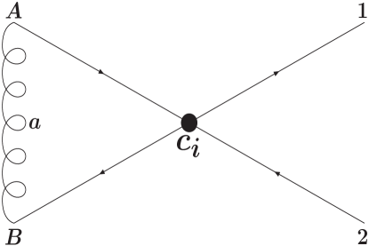
Figure 2.1: The diagram obtained by dressing the colour tensor $c_{i}$ with a virtual gluon $a$ which connects external legs $A$ and $B$, for the process $q(A)\,\bar{q}(B)\rightarrow q(1)\,\bar{q}(2)$. In the notation in the text, this diagram is denoted $\mathcal{C}_{i}^{(AB)}$. Note that in this section we are only concerned with the colour flow, and not the dynamics, of this diagram.

Now we turn to the cases of diagrams involving $c_{2}$. Starting with $\mathcal{C}_{2}^{(12)}$ we have

$$\mathcal{C}_{2}^{(12)} = t^{a}_{Bn}\,c_{2}\,t^{a}_{mA},$$ (2.20)

$$= t^{a}_{Bn}\,\frac{1}{2}\left(\delta_{mn}\delta_{12}-\frac{1}{N_{c}}\delta_{m1}\delta_{n2}\right)\,t^{a}_{mA}.$$

If we expand the terms, then we can use equation (2.19) on the first term and equation (2.15) on the second to obtain

$$\mathcal{C}_{2}^{(12)}=\frac{C_{F}}{2N_{c}}c_{1}+\left(C_{F}-\frac{1}{2N_{c}}\right)c_{2}.$$ (2.21)

A similar calculation for the other classes of diagram yields,

$$\mathcal{C}^{(A1)}_{2} = \mathcal{C}^{(B2)}_{2}=-\frac{1}{2N_{c}}c_{2},$$

$$\mathcal{C}^{(B1)}_{2} = \mathcal{C}^{(A2)}_{2}=-\frac{1}{N_{c}}c_{2}+\frac{C_{F}}{2N_{c}}c_{1}.$$ (2.22)

We can now write down the mixing matrix for this process in terms of the three classes of diagram, and we use $\alpha$, $\beta$ and $\gamma$ to denote the associated dynamical piece, $\zeta^{(ij)}$, of the relevant diagram,

$$\alpha=\zeta^{(AB)}+\zeta^{(12)},$$

$$\beta=\zeta^{(A1)}+\zeta^{(B2)},$$

$$\gamma=\zeta^{(B1)}+\zeta^{(A2)}.$$ (2.23)

We will use this notation, and discuss the origin of the dynamical pieces, in chapter 6. Recall that if the undressed set is denoted $(c_{1},c_{2})^{T}$ and the set which has mixed under quantum corrections is denoted $(c_{1}^{\prime},c_{2}^{\prime})^{T}$, then

$$\left(\begin{array}[c]{c}c_{1}^{\prime}\\ c_{2}^{\prime}\end{array}\right)=C^{q\bar{q}\rightarrow q\bar{q}}\left(\begin{array}[c]{c}c_{1}\\ c_{2}\end{array}\right),$$ (2.24)

where the mixing matrix, $C^{q\bar{q}\rightarrow q\bar{q}}$, is given by

$$\mathcal{C}^{q\bar{q}\rightarrow q\bar{q}}=\left(\begin{array}[c]{cc}C_{F}\beta&\frac{C_{F}}{2N_{c}}(\alpha+\gamma)\\ \alpha+\gamma&C_{F}\alpha-\frac{1}{2N_{c}}(\alpha+\beta+2\gamma)\end{array}\right).$$ (2.25)

This matrix describes how the colour tensors, and the associated dynamical pieces, mix under quantum corrections. The mixing matrix for the other quark process, $qq\rightarrow qq$, can be calculated in a similar way and appears in appendix F.

2.3.2 The addition of gluons

The presence of external gluons increases the complexity of the colour mixing calculations, due to more involved group theory. In this section we will describe the calculation of the mixing matrix for the process $q(A)\,g(B)\rightarrow q(1)\,g(2)$, which will introduce the majority of the tools needed for the gluon processes. The basis for this process is

$$c_{1} = \delta_{A1}\delta_{B2},$$

$$c_{2} = d_{B2c}(t_{F}^{c})_{1A},$$

$$c_{3} = if_{B2c}(t^{c}_{F})_{1A},$$ (2.26)

where the first element describes singlet exchange, and the second and third members describe symmetric and antisymmetric colour exchange respectively. The constants $f^{ABC}\,(A,B,C=1,\dots,8)$ are the antisymmetric structure constants of SU(3). They are antisymmetric under the exchange of any two indices and satisfy the Jacobi identity,

$$f_{ABE}f_{ECD}+f_{CBE}f_{AED}+f_{DBE}f_{ACE}=0.$$ (2.27)

The constants $d^{ABC}\,(A,B,C=1,\dots,8)$ are the symmetric structure constants of SU(3). They are symmetric under the exchange of any two indices, obey $d_{ABB}=0$ and satisfy

$$f_{ABE}d_{ECD}+f_{CBE}d_{AED}+f_{DBE}d_{ACE}=0.$$ (2.28)

From these, and the group theory identities in appendix A, from which we mainly use

$$t^{a}_{ij}t^{b}_{jk}=\frac{1}{2}\left[\frac{1}{N_{c}}\delta_{ab}\delta_{ik}+\left(d_{abc}+if_{abc}\right)t^{c}_{ik}\right],$$ (2.29)

we can deduce the following basis relationships,

$$c_{3}\times c_{1} = c_{3},$$ (2.30)

$$c_{2}\times c_{1} = c_{2},$$ (2.31)

$$c_{3}\times c_{2} = -\frac{N_{c}}{4}c_{2}+\frac{N_{c}^{2}-4}{4N_{c}}c_{3},$$ (2.32)

$$c_{3}\times c_{3} = \frac{1}{2}c_{1}+\frac{N_{c}}{4}c_{2}-\frac{N_{c}}{4}c_{3},$$ (2.33)

which are useful when we see that adding a virtual t-channel soft gluon to the colour tensor $c_{i}$ is equivalent to taking the tensor product of this colour tensor with $c_{3}$. These identities are straightforward to prove; for example, if we label the two exchanged gluons as $c$ and $d$, the virtual quark as $i$ and the virtual gluon as $j$, we get the following group algebra for $c_{3}\times c_{3}$,

$$c_{3}\times c_{3}=if^{Bjc}\,t^{c}_{iA}\times if^{j2d}\,t^{d}_{1i},$$ (2.34)

where we can see the meaning of the $\times$ notation. By using equation (2.29) and equations (A.10-A.16) we can prove equation (2.33). We can now use these identities and deduce that

$$\mathcal{C}_{1}^{(AB)} = c_{3},$$ (2.35)

$$\mathcal{C}_{2}^{(AB)} = c_{3}\times c_{2}=-\frac{N_{c}}{4}c_{2}+\frac{N_{c}^{2}-4}{4N_{c}}c_{3},$$ (2.36)

$$\mathcal{C}_{3}^{(AB)} = c_{3}\times c_{3}=\frac{1}{2}c_{1}+\frac{N_{c}}{4}c_{2}-\frac{N_{c}}{4}c_{3},$$ (2.37)

and $\mathcal{C}_{i}^{(12)}=\mathcal{C}_{i}^{(AB)}$. Hence

$$\mathcal{C}_{i}^{(12)}=\mathcal{C}_{i}^{(AB)}=\left(\begin{array}[c]{ccc}0&0&\frac{1}{2}\\ 0&-\frac{N_{c}}{4}&\frac{N_{c}}{4}\\ 1&\frac{N_{c}-4}{4N_{c}}&-\frac{N_{c}}{4}\end{array}\right).$$ (2.38)

Turning now to $\mathcal{C}^{(A1)}$, we see that

$$\mathcal{C}_{1}^{(A1)}=C_{F}c_{1},$$ (2.39)

and that

$$\mathcal{C}_{2}^{(A1)} = d_{B2c}\,t^{c}_{ji}\,t^{d}_{iA}\,t^{d}_{1j},$$ (2.40)

$$= d_{B2c}\,t^{c}_{ji}\,\frac{1}{2}\left(\delta_{ij}\delta_{A1}-\frac{1}{N_{c}}\delta_{iA}\delta_{1j}\right),$$

$$= -\frac{1}{2N_{c}}d_{B2c}\,t^{c}_{1A},$$

$$= -\frac{1}{2N_{c}}c_{2},$$

where we have expanded the pair of SU(3) matrices $t^{d}_{iA}\,t^{d}_{1j}$ and used the fact that $t^{a}_{ii}=0$. Finally, working in a similar way,

$$\mathcal{C}_{3}^{(A1)} = if_{B2c}\,t^{c}_{ji}\,t^{d}_{1j}\,t^{d}_{iA},$$ (2.41)

$$= -\frac{1}{2N_{c}}c_{3}.$$

Note that these last three results are not the same for $\mathcal{C}^{(B2)}$. For this case the group algebra gives (where we note that $N_{c}=C_{A}$),

$$\mathcal{C}_{1}^{(B2)} = if_{Bdc}\,if_{d2c}\,\delta_{A1}=C_{A}c_{1},$$ (2.42)

$$\mathcal{C}_{2}^{(B2)} = t^{d}_{1A}\,d_{ijd}\,if_{Bic}\,if_{j2C}=\frac{N_{c}}{2}c_{2},$$ (2.43)

$$\mathcal{C}_{3}^{(B2)} = -t^{d}_{1A}\,f_{ijd}\,f_{Bic}\,f_{j2C}=\frac{N_{c}}{2}c_{3}.$$ (2.44)

For the first of these results we have used the fact that $f_{Bcd}\,f_{2cd}=N_{c}\delta_{B2}$, for the second of these results we have used the fact that $d_{jdi}\,f_{iBc}\,f_{c2j}=-d_{B2d}$ and for the third of these results we have used the fact that $f_{jdi}\,f_{iBc}\,f_{c2j}=-\frac{N_{c}}{2}f_{db2}$. Therefore we find that

$$\mathcal{C}_{i}^{(A1)} = \left(\begin{array}[c]{ccc}C_{F}&0&0\\ 0&-\frac{1}{2N_{c}}&0\\ 0&0&-\frac{1}{2N_{c}}\end{array}\right),$$ (2.48)

$$\mathcal{C}_{i}^{(B2)} = \left(\begin{array}[c]{ccc}C_{A}&0&0\\ 0&\frac{N_{c}}{2}&0\\ 0&0&\frac{N_{c}}{2}\end{array}\right).$$ (2.52)

After similar, albeit longer, calculations we find

$$c_{1}^{(A2)} = c_{3},$$ (2.53)

$$c_{2}^{(A2)} = id_{j2c}\,f_{Bjd}\,t^{d}_{1i}\,t^{c}_{iA}=\frac{N_{c}^{2}-4}{4N_{c}}c_{3}+\frac{N_{c}}{4}c_{2},$$ (2.54)

$$c_{3}^{(A2)} = -f_{j2c}\,f_{Bjd}\,t^{d}_{1i}\,t^{c}_{iA}=\frac{1}{2}c_{1}+\frac{N_{c}}{4}c_{2}+\frac{N_{c}}{4}c_{3},$$ (2.55)

and hence the result

$$\mathcal{C}_{i}^{(A2)}=\mathcal{C}_{i}^{(B1)}=\left(\begin{array}[c]{ccc}0&0&\frac{1}{2}\\ 0&\frac{N_{c}}{4}&\frac{N_{c}}{4}\\ 1&\frac{N_{c}^{2}-4}{4N_{c}}&\frac{N_{c}}{4}\end{array}\right),$$ (2.56)

and so we find the colour mixing matrix for the process $qg\rightarrow qg$, in basis 2.26, is

$$\mathcal{C}^{qg\rightarrow qg}=\left(\begin{array}[c]{ccc}C_{F}\mathcal{C}^{(A1)}+C_{A}\mathcal{C}^{(B2)}&0&-\frac{1}{2}(\alpha+\gamma)\\ 0&\chi&-\frac{N_{c}}{4}(\alpha+\gamma)\\ -(\alpha+\gamma)&-\frac{N_{c}^{2}-4}{4N_{c}}(\alpha+\gamma)&\chi\end{array}\right),$$ (2.57)

where

$$\chi=\frac{N_{c}}{4}(\alpha-\gamma)-\frac{1}{2N_{c}}\zeta^{(A1)}+\frac{N_{c}}{2}\zeta^{(B2)}.$$ (2.58)

In this equation, as in the previous section, $\zeta^{(ij)}$ denotes the dynamical piece of the relevant diagram. We can proceed in a similar way and calculate the mixing matrices for any partonic process that may interest us. The bases and the mixing matrices for all the processes used in this thesis can be found in appendices D and F and we will use these results when we study the resummation of rapidity gap events in chapters 4 and 6.

2.4 Regge theory and the pomeron

Regge theory [10] provides a framework to describe scattering amplitudes in the Regge limit $s\gg-t$. Whilst in this thesis we are primarily concerned with the perturbative description of rapidity gap processes, we will use some of the ideas of Regge theory in chapter 3 to examine diffractive processes and so in this section we will outline some of the basic concepts. Further details can be found in [11, 12, 13].

The whole idea of Regge theory, starting from the analytic properties of the S-matrix, is to extract the high energy behaviour of scattering amplitudes in a model independent way. The fundamental result is that the dominant contribution to the high energy scattering amplitude has a general form, which has the interpretation of the exchange of objects known as reggeons in the t-channel. It can be shown that if the high energy cross section in the Regge region can be described only in terms of reggeon exchanges, then the total cross section will behave like

$$\sigma_{\mathrm{tot}}\propto s^{\alpha(0)-1},$$ (2.59)

where $\alpha(0)$ is known as the intercept of the Regge trajectory (the Regge trajectory is a straight line in the spin-mass squared plane of the exchanged mesons). The fits of Chew and Frautschi [14] to meson data showed that $\alpha(0)=0.55$, and this observation of $\alpha(0)<1$ was found to be true for other exchange particles. Hence the total cross section should decrease with $s$, and vanish asymptotically. However when the total cross section was measured experimentally, it was found that it slowly increased at high $s$. Therefore reggeon exchange is not the whole story, and a new trajectory is needed to describe the data, with an intercept greater than unity, $\alpha(0)>1$. This new trajectory is known as the pomeron trajectory, or the pomeron.

From fits to total $pp$ and $p\bar{p}$ data, Donnachie and Landshoff [15] extracted the pomeron intercept and found

$$\alpha(0)\simeq 1.08.$$ (2.60)

This is normally known as the “soft” pomeron intercept. We will use the ideas of Regge theory in chapter 3, when we study diffractive processes at the Tevatron and we will describe the diffractive interaction of two hadrons by the exchange of both pomerons and reggeons.

2.5 Event generators

Monte Carlo event generators have many uses in particle physics, for example estimating the backgrounds to measured processes and calculating production rates of exotic particles. In this thesis we will use the Monte Carlo event generator HERWIG [16, 17] on two occasions as a calculation tool and in this section we will give an overview of the theoretical methods used. Our discussion in this section on Monte Carlo event generators will hence refer to the operation of HERWIG.

The idea of a Monte Carlo event generator is to give a simulation of a particle physics event, starting from the initial interaction of the colliding particles and culminating in the angular distribution and energy of (colourless) final state particles. This is still a level removed from what is seen in particle detectors, and the inclusion of detector effects is possible, but it is largely sufficient for the research work in the following chapters. To simulate the event, HERWIG starts with a hard subprocess and evolves the resulting off-shell partons into colourless final state particles; to do this HERWIG is separated into a number of distinct phases.

For the process of two hadrons interacting to produce a number of hadronic jets, HERWIG starts by calculating the hard subprocess, producing two final state partons using the QCD factorisation theorems with a leading order calculation and the parton distribution functions of the hadrons. At this point we have selected a QCD $2\rightarrow 2$ subprocess, but any perturbatively calculable process of the standard model or any of its extensions is permissible. The result of the calculation is two initial state and two final state partons, with their associated 4-momenta, and the total cross section for the process, which is calculated by evaluating the integral,

$$\sigma^{\mathrm{hard}}(s,p_{t,\mathrm{min}})=\int_{p^{2}_{t,\mathrm{min}}}^{s/4}dp_{t}^{2}\int\frac{d\sigma^{\mathrm{hard}}(s)}{dx_{1}\,dx_{2}\,dp_{t}^{2}}dx_{1}\,dx_{2},$$ (2.61)

where $p_{t}$ is the transverse momentum of the outgoing partons. The cut $p_{t,\mathrm{min}}$ is necessary to prevent the integrand approaching divergences in the matrix element and the Landau pole in the coupling.

Once the momenta of the final state partons produced by the hard event have been generated, the initial and final state partons are evolved through perturbative branching, and all emitted partons are themselves evolved, until all partons reach an infrared hadronisation scale which characterises the onset of non-perturbative physics.

Final state parton shower

The off-shell partons produced by the hard subprocess subsequently evolve with the emission of QCD radiation. The exact calculation of the matrix element for processes with many final state particles is not possible, and we must use a branching algorithm which correctly takes into account the regions of phase space in which QCD radiation is enhanced. These regions are associated with kinematical configurations in which the relevant matrix elements are enhanced, and correspond to emission of a soft gluon, or when a gluon or a quark splits into two collinear partons. The aim of a parton shower algorithm is to identify and sum up the leading behaviour in these regions.

The parton showering is controlled by a set of Sudakov form factors, which encode the probability that a parton with a virtual mass scale $t$ will evolve without resolvable branching to the lower virtual mass scale $t_{1}$. If branching does occur, splitting functions are used to compute the momentum fraction and virtual mass scale of the products. The Sudakov form factors take into account collinear enhancements and also soft enhancements using the coherent branching formalism and the parton shower is terminated when all partons reach the cut-off scale $t_{0}$. The virtual mass scale variable, $t$, which is evolved to $t_{0}$, is a combination of parton energy and branching opening angle; this choice of the evolution variable is the correct one to include both soft and collinear enhancements. There is an excellent explanation of the parton shower formalism, and the application to Monte Carlo event generators, in [1, 18].

Initial state parton shower

The final state parton shower is called a forward evolution algorithm, as in every step the partons move to a lower virtual mass scale. For the initial state parton shower, it is more convenient to start with the (most negative virtual) partons which particpate in the hard event and evolve backward to the lower virtual mass scales of the partons in the interacting hadrons. In this backward evolution formalism, the parton distribution functions are used as part of the input, to “guide” the evolution to the correct distribution of partons.

Hadronisation

Using the parton shower formalism, all partons are evolved until they reach the cut-off scale $t_{0}$. It is at this point that we enter the long-wavelength, non-perturbative regime where the partons group themselves into the colourless hadrons we observe; this process is included in HERWIG using a phenomenological model.

A property of the parton showering is that the flow of momentum and quantum numbers at the hadron level tends to follow the flow at the parton level. This hypothesis is known as local parton-hadron duality (LPHD), and underlies the cluster hadronisation model [19, 20] used by HERWIG. In this model, clusters of colour singlet partons form after the parton shower, inheriting the momentum structure of their constituent partons. The process occurs by the splitting of gluons into quark/antiquark pairs, and then neighbouring quarks and antiquarks form colour singlet objects. Unstable hadrons are then allowed to decay according to experimentally determined branching ratios and this process, which tends to disfavour heavy mesons and baryons, provides a good model of observed final states in $e^{+}e^{-}$ collisions.

HERWIG also includes a model of the underlying soft event, in which the hadron remnants undergo secondary soft interactions. Once the final state has been determined, the experimental cuts for the analysis of interest can be applied and observables calculated. It is also possible, as we briefly mentioned earlier, to add a further phase of detector simulation, where the experimental signature of the produced final state is simulated. Such a process allows for detailed comparisons to be made with experimental observation.

We will use HERWIG in chapter 3, where we are especially interested in the effects of parton showering and hadronisation and again in chapter 6, where we will be interested in the computation of the hard event.

2.6 Rapidity gaps

The aim of this thesis is to examine the physics of rapidity gap processes, and make predictions to compare to recent experimental data; in this section we will give a brief overview of rapidity and rapidity gaps in particle collisions. The scattering of two hadrons provides two beams of incoming partons, with a spectrum of longitudinal momenta described by hadronic parton densities. The parton centre-of-mass frame is boosted with respect to the incoming hadron frame, and it is natural to describe the final state in terms of variables which have simple transformation properties under longitudinal boosts. To do this we describe the final state in terms of transverse momentum $p_{t}$, rapidity $y$ and azimuthal angle $\phi$, and a general 4-vector is written

$$p^{\mu} = (E,p_{1},p_{2},p_{3}),$$ (2.62)

$$= \left(m_{t}\cosh y,p_{t}\sin\phi,p_{t}\cos\phi,m_{t}\sinh y\right),$$

where we define the transverse mass for a particle of mass $m$ by $m_{t}=\sqrt{p_{t}^{2}+m^{2}}$. Rapidity is defined as

$$y = \frac{1}{2}\log\left(\frac{E+p_{3}}{E-p_{3}}\right),$$ (2.63)

$$= \frac{1}{2}\log\left(\frac{1+v\cos\theta}{1-v\cos\theta}\right),$$ (2.64)

and is a measure of polar angle and speed.

Pseudorapidity is often more useful in practice, which is defined

$$\eta=-\log\tan\left(\frac{\theta}{2}\right).$$ (2.65)

Rapidity and pseudorapidity coincide in the massless limit, but pseudorapidity is more convenient in that the polar angle $\theta$ can be measured directly from the detector and we require no knowledge of the particle mass. Rapidities (and approximately pseudorapidities) are additive under z-axis Lorentz boosts, and (pseudo)rapidity differences,

$$\Delta\eta=|\eta_{1}-\eta_{2}|,$$ (2.66)

are boost invariant.

Figure 2.2: The experimental signature of a “gap-jet-gap” event. The dark circles denote two jets, and the gap regions are separated from the central dijet system by the dashed lines.

A rapidity gap event is defined as an event producing jets, with the region in pseudorapidity between any two jets, $\Delta\eta$, being devoid of particle activity. This interjet region, known as a gap, is often symmetrical in azimuthal angle $\phi$. The precise definition of the gap depends on the experimental geometry, and is experimentally defined by a cut on the total transverse energy flowing in the gap region. In this thesis we will consider two kinds of rapidity gap processes:

• “gap-jet-gap” processes in diffractive hadron collisions. In this class of process, the final state consists of a central (in rapidity) dijet system, separated from the intact colliding hadrons by a rapidity gap on each side. Hence the “gap-jet-gap” experimental signature, which is illustrated in figure 2.2. We shall study these processes in chapter 3, where the rapidity gap is produced by the exchange of a pomeron between the hadron and the central system.

• “jet-gap-jet” processes in photoproduction. In this class of process we see a rapidity gap between the two dijets. We shall study these gaps-between-jets processes in chapters 4, 5 and 6, where we will make perturbative calculations of the rate of gap-event production and make comparisons to experimental data. The experimental signature is illustrated in figure 2.3.

For both classes of rapidity gap process, we will find that the predictions of the methods that we use will give a good description of the data.

Figure 2.3: The experimental signature of a “jet-gap-jet” event. The dark circles denote two jets, and the gap region is bounded by the dashed lines.

2.7 Summary

In this chapter we have outlined some of the tools we shall be using in this thesis. The features of asymptotic freedom and factorisation give QCD immense predictive power, and one of the central aims of our work is to examine the consequences of factorisation for the perturbative calculation of rapidity gap processes at HERA. An important element of our calculations will be colour mixing, and in section 2.3 we derived a set of process-dependent QCD mixing matrices for a fixed basis. We will use these matrices in chapter 6. We then described the basic ideas of Regge theory, event generators and rapidity gaps, in preparation for the use of these ideas in our calculations. So in conclusion, the research work in this thesis deals with the calculation of rapidity gap processes in QCD and builds on the fundamental tools presented in this chapter.

Chapter 3 Diffractive dijet production

3.1 Introduction

In this chapter we will study hard diffractive processes in hadron-hadron collisions. To be specific we will make detailed calculations for the process $p\bar{p}\rightarrow p+JJX+\bar{p}$, where $JJX$ denotes a centrally produced cluster of hadrons, containing at least two jets. The process is theoretically diffractive in the sense that both the initiating hadrons remain intact in the collision and experimentally diffractive in the sense that the initiating proton remains intact, whilst the antiproton either remains intact or dissociates to a low-mass system. In both cases the initiating hadrons suffer only a small loss of longitudinal momentum, and the process is hard in the sense that the central subprocess takes place at high momentum transfer. The central (in rapidity) jet-producing system is separated by a rapidity gap from each of the interacting hadrons, giving the experimental signature of “gap-jet-gap” events and the term hard double diffraction.

Space-time arguments [21] suggest that hard events are well localised in space and time, and therefore the effect of the incoming particles is to act independently of the hard event. This has led, in analogy to conventional QCD factorisation theorems, to the concept of a diffractive parton density and the hard diffractive factorisation theorems. Diffraction factorisation has been proven for diffractive DIS, but for hard diffraction in pure hadron collisions counterarguments exist which predict that the factorisation will be violated at the Tevatron [22, 21, 23, 24]. The manifestation of this violation is the invalidity of using diffractive parton densities, obtained in DIS experiments at HERA, in hadron-hadron collisions at the Tevatron and we should expect to see an overestimation of predicted cross sections. The extent of the breakdown of factorisation is still under investigation and has been embodied in so-called gap survival factors, which will have direct relevance in this work.

The standard factorised model of double diffraction draws its inspiration from Regge theory. In the Ingelman-Schlein (IS) model [25], diffractive scattering is attributed to the exchange of a pomeron, which is defined as a colourless object with vacuum quantum numbers. The model assumes that each of the diffracting hadrons “emits” a pomeron, which then collide to produce the central dijet system. This is illustrated in figure 3.1. Implicit in the model is Regge factorisation, which writes a diffractive parton density as the product of the pomeron parton density and a pomeron flux factor. The double diffractive process then proceeds by the QCD interactions of the emitted pomerons. This kind of event mechanism is known as double pomeron exchange.

In this chapter we will use the Ingelman-Schlein model of double diffraction to make predictions for gaps-between-jets processes at the Tevatron. The CDF collaboration has recently presented analyses of such events [26]. We will include the effects of fragmentation using the diffractive event generator POMWIG [27], and use the pomeron parton densities from HERA DIS experiments [28]. Previous calculations of this type of event [22, 29] have led to an overestimation of the dijet production cross section by several orders of magnitude. In this chapter we will show that a combination of the HERA parton densities and a gap survival factor [30] consistent with theoretical estimates [31, 32] is sufficient to describe the recent CDF data. Central dijet production within a factorised model has been studied before [22, 29, 33, 34] and the research work in this chapter is published in [35].

This chapter is organised as follows. We start by introducing the experimental analyses in section 3.2, and section 3.3 is a detailed discussion of the IS model and the concept of diffractive parton densities. Section 3.4 then discusses the diffractive event generator POMWIG, and how it is constructed from HERWIG, and section 3.5 gives our results. Finally, in section 3.6, we draw our conclusions.

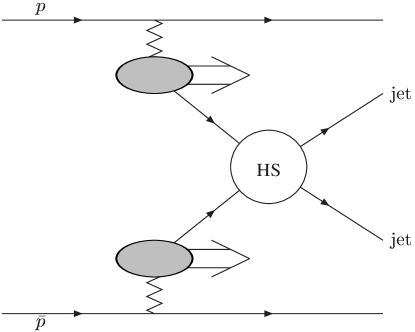
Figure 3.1: Dijet production in the factorised model. The zig-zag lines denote the exchanged pomerons, and the double-lined arrows represent the pomeron remnants.

3.2 Diffractive dijet production at the Tevatron

The first observation at the Tevatron of dijet events with a double pomeron exchange topology was published in 2000 by the CDF collaboration [26]. In this section we will describe the experimental signature of these events, the observables and cuts used, and finish with a description of the out-of-cone corrections implemented by CDF to “undo” the jet broadening effects of fragmentation.

3.2.1 Diffractive events and the CDF analysis

The diffractive data used in this work was collected by the CDF collaboration when the Tevatron was colliding protons and antiprotons at a centre-of-mass energy $\sqrt{s}=1800$ GeV. The events were obtained by making a further analysis of the single diffractive (SD) data set; SD meaning that only one interacting hadron undergoes diffraction. In this analysis, events with a rapidity gap on the antiproton side were selected by requiring a fractional momentum loss of the antiproton, $\xi_{\bar{p}}$, to satisfy $0.035<\xi_{\bar{p}}<0.095$, by detecting the antiproton in a forward Roman Pot Spectrometer (RPS). The requirement was then made of at least two centrally produced jets of transverse energy $E_{T}^{\mathrm{min}}>7$ GeV and a 4-momentum transfer from the antiproton squared of $|t|<1$ GeV². This SD sample (of 30,439 events) was then used to search for double diffractive events by demanding a rapidity gap on the proton side. There is no RPS on this side of the CDF detector and the events were selected by directly demanding a region devoid of particle activity in the pseudorapidity region between the central dijet system and the outgoing proton. This method is not a very accurate way to determine whether a given event is indeed a genuine double diffractive event, and consequently gives a large uncertainty on the the fractional momentum loss, $\xi_{p}$, of the proton. As a result, CDF found that the $\xi_{p}$ distribution was concentrated in the region $0.01<\xi_{p}<0.03$ and used this region for the $\xi_{p}$ cut. The subset of the SD sample satisfying this criteria is the double diffractive sample (denoted DD, in which two interacting hadrons undergo diffraction). The double diffractive experimental signature is illustrated in figure 3.2.

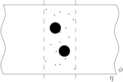
Figure 3.2: The experimental signature of a “gap-jet-gap” event. The dark circles denote two jets, and the gap regions are separated from the central dijet system by the dashed lines.

In summary, the CDF cuts used to select the double pomeron exchange events were

• The antiproton fractional energy loss $\xi_{\bar{p}}$ satisfies $0.035<\xi_{\bar{p}}<0.095$. Such a condition corresponds to a rapidity gap on the antiproton side. This cut is made by tagging the antiproton.

• The proton fractional energy loss $\xi_{p}$ satisfies $0.01<\xi_{\bar{p}}<0.03$. Such a condition corresponds to a rapidity gap on the proton side. Note that the proton is not tagged at CDF and the cut is made by looking for a rapidity gap on the proton side.

• $|t_{\bar{p}}|<1$ GeV². $|t_{\bar{p}}|$ is the four-momentum transfer from the antiproton squared.

• The event must have two or more jets in the pseudorapidity region

  $$-4.2<\eta<2.4,$$ (3.1)

  and at least two jets must have a minimum transverse energy of $E_{T}^{min}=7~{}$ GeV or $10$ GeV. The CDF collaboration define the outgoing proton direction as the positive $\eta$ direction, also known as “East”.

The CDF analyses presented the total dijet cross section at $E_{T}^{min}>7$ GeV and $E_{T}^{min}>~{}10$ GeV. They also presented event distributions in $\xi_{p}$, $\xi_{\bar{p}}$, the mean jet transverse energy $E_{T}^{*}$, the mean jet rapidity $\eta^{*}$, the azimuthal angle separation of the dijets and the dijet mass fraction $R_{jj}$. The last quantity is defined as the mass of the dijet system evaluated using only the energy within the cones of the two leading jets, $M_{jj}^{\mathrm{cone}}$, divided by the mass of the central system, $M_{x}=\sqrt{s\xi_{p}\xi_{\bar{p}}}$.

3.2.2 Jet finding and the cone algorithm

The classification of a hadronic final state into one or more “jets” of hadronic particles is a task performed by a jet algorithm. Modern algorithms have their roots in the Sterman-Weinberg jet definition [36], and today several different algorithms exist. The method used by the CDF collaboration in their double diffractive dijet production analyses was the cone definition. In this algorithm, a jet is defined as the concentration of all particles inside a cone of $(\eta,\phi)$ space, of radius $R$ in the $(\eta,\phi)$ plane,

$$R=\sqrt{(\Delta\eta)^{2}+(\Delta\phi)^{2}}.$$ (3.2)

The jets are reconstructed to place as much of the transverse energy as possible inside a cone, with a minimum energy of $\epsilon^{\mathrm{cut}}$ GeV. Overlapping cones are handled by excluding jets with more than a certain fraction, normally known as the overlap parameter, of their energy coming from other jets. By defining $R$ in terms of $\Delta\eta$ (other choices could be in terms of $\Delta\theta$, for example) we obtain a jet measurement invariant under longitudinal boosts. Note that any cross section is dependent on the choice of the cone radius $R$. In this work we will follow CDF and set $R=0.7$. Figure 3.3 shows the application of the cone algorithm to a 3 jet event at the Tevatron. The clusters of particles defined as a jet are ringed by the cone radius in this figure.

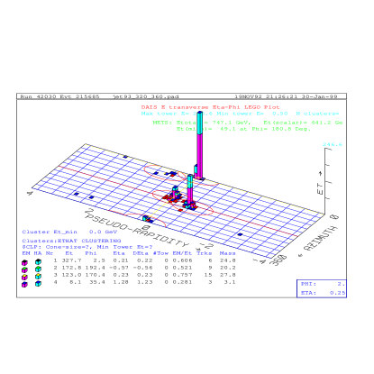
Figure 3.3: A 3 jet event, defined using the cone algorithm with $R=0.7$, from the CDF experiment. The clusters of particles defined as a jet are ringed by the cone radius. This figure is taken from [38] with the authors’ permission.

Once a concentration of particles has been identified as a jet, the transverse energy of that jet is given by the sum of all the transverse energies of the constituent particles,

$$E_{T}^{\mathrm{jet}}=\sum_{i\in\mathrm{jet}}E_{T}^{i}.$$ (3.3)

Other kinematic variables have similar definitions, of which

$$\eta^{\mathrm{jet}}=\frac{\sum_{i\in\mathrm{jet}}E_{T}^{i}\,\eta^{i}}{E_{T}^{\mathrm{jet}}},$$

$$\phi^{\mathrm{jet}}=\frac{\sum_{i\in\mathrm{jet}}E_{T}^{i}\,\phi^{i}}{E_{T}^{\mathrm{jet}}},$$ (3.4)

is one possible form.

3.2.3 Out-of-cone corrections

The CDF collaboration have applied so-called out-of-cone (oc) corrections to the diffractive dijet data sample. These corrections are applied as the jet clustering algorithm may not include all of the energy from the initiating partons, and some of the partons generated during fragmentation may fall outside of the jet algorithm cones. Therefore the out-of-cone corrections add transverse energy to the jets to account for this missing $p_{t}$ and “correct” the particle-level jet energies back to the parton level. This procedure (which is difficult to justify) means that CDF no longer presents a true observable. These corrections depend on the parton fragmentation functions, and are totally independent of the CDF detector. The out-of-cone corrections take the form of a simple addition to the jet $p_{t}$, and were derived from Run I data. The additional energy is given by

$$p_{t}^{+}=A(R)\left(1-B(R)e^{-C(R)p_{t}}\right),$$ (3.5)

where $p_{t}$ is the particle-level jet energy and the functions $A(R)$,$B(R)$ and $C(R)$ depend on the cone radius ($R$) and have the values given in table 3.1.

	A [GeV]	B	C [GeV-1]
0.4	22.999	0.915	0.00740
0.7	8.382	0.846	0.00728
1.0	3.227	0.832	0.00817

Table 3.1: The out-of-cone correction parameters, as derived from Run I Tevatron data [39]. We have shown the out-of-cone correction parameters for three different values of the radius, although only $R=0.7$ is relevant to the current work.

The impact of the out-of-cone corrections to the work in this chapter is that it is necessary to implement the out-of-cone corrections in the Monte Carlo simulation and compare the hadron level Monte Carlo cross sections with the corrections to the CDF data, and not (as it may first appear) compare the data to the hadron level cross sections. Nevertheless, the use of Monte Carlo event generators allows the impact of the fragmentation process to be assessed.

3.3 Diffractive factorisation and the Ingelman-Schlein model

We will now examine the mechanisms for hard double pomeron exchange dijet production. In this work we will use the factorised Ingelman-Schlein model, which takes its inspiration from Regge theory. We will also describe the non-factorised model of lossless jet production [23, 40, 41, 42], but we will not make any calculations using this model in this thesis.

3.3.1 Hard diffraction

The pomeron is the object thought to be responsible for rapidity gap processes. Defined as an exchanged object carrying the quantum numbers of the vacuum, it is postulated to exist in many forms - from the soft pomeron of Regge theory to the perturbative QCD pomeron embodied by the famous Balitsky-Fadin-Kuraev-Lipatov (BFKL) equation. Close to 20 years ago Ingelman and Schlein proposed that it was possible to probe the content of the pomeron by looking at the diffractive production of high $p_{t}$ dijets. In so-called hard diffraction the momentum transfer across the rapidity gap is small, with the gap corresponding to the exchange of a colour singlet object, but a high $Q^{2}$ process occurs between the exchanged object and the other hadron. This is be contrasted with diffractive hard scattering, in which the colour singlet object is exchanged with a high momentum transfer across the gap. Therefore the basic idea of Ingelman and Schlein [25] is that the exchange mechanism for the pomeron is the same for hard diffraction and soft diffraction, and the pomeron interacts through its partonic constituents. These ideas took shape when looking at single diffraction, $\bar{p}+p\rightarrow\bar{p}+X$, and led to the following picture:

• The diffracting antiproton will emit a pomeron with a small momentum transfer $t$. The pomeron is sometimes said to “float” out of the “parent” antiproton.

• The pomeron, carrying a partonic content, then interacts with the partons in the proton at high $Q^{2}$.

The standard Regge single diffractive cross section (single diffraction with a diffracted proton) is

$$\frac{d^{2}\sigma_{SD}^{\bar{p}p}}{d\xi dt}=f_{\mathbb{P}/p}(\xi,t)\sigma_{t}^{\mathbb{P}\bar{p}}(s^{\prime},t),$$ (3.6)

where $s^{\prime}=s\xi$ is the centre-of-mass energy of the pomeron-antiproton system, $\sigma_{t}^{\mathbb{P}\bar{p}}(s^{\prime},t)$ is the total pomeron-proton cross section ($\sigma(p\mathbb{P}\rightarrow X)$) and $f_{\mathbb{P}/p}(\xi,t)$ is the pomeron flux factor. We have illustrated this Regge factorisation of the cross section in figure 3.4.

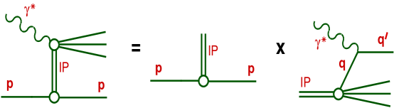
Figure 3.4: An illustration of Regge factorisation. Figure from [43].

This equation can be treated as a definition of the pomeron flux, and allows us to write the single hard diffractive cross section for the production of dijets as,

$$\frac{d^{4}\sigma^{jj}_{SD}}{dx_{\mathbb{P}}dtdx_{1}dx_{2}}=\left[\frac{1}{\sigma(p\mathbb{P}\rightarrow X)}\frac{d^{2}\sigma_{SD}}{dx_{\mathbb{P}}dt}\right]\frac{d^{2}\sigma(p\mathbb{P}\rightarrow jj+X)}{dx_{1}dx_{2}},$$ (3.7)

where $x_{\mathbb{P}}$ is the momentum loss fraction of the antiproton (i.e. momentum fraction of the pomeron to the antiproton), $t$ is the 4-momentum transfer-squared and $\sigma(p\mathbb{P}\rightarrow jj+X)$ is the proton-pomeron hard-scattering cross section. The pomeron flux factor (in square brackets) depends on $x_{\mathbb{P}}$ and $t$. The pomeron-proton hard scattering cross section depends on the momentum fractions, $x_{1}$ and $x_{2}$, of partons in the parton and the pomeron respectively. Therefore this differential cross section is given by

$$\frac{d^{3}\sigma(p\mathbb{P}\rightarrow jj+X)}{dx_{1}dx_{2}dQ^{2}}=\sum_{i,j}f_{i/p}(x_{1},Q^{2})f_{j/\mathbb{P}}(x_{2},Q^{2})\frac{d\sigma(ij\rightarrow\mathrm{dijets})}{dQ^{2}},$$ (3.8)

where $f_{i/p}(x_{1},Q^{2})$ and $f_{j/\mathbb{P}}(x_{2},Q^{2})$ are the parton densities of the proton and the pomeron respectively. In the original IS model it was assumed that the pomeron was a purely gluonic object with a parton density that was $Q^{2}$ and $t$ independent, and two simple forms where proposed,

$$xf_{g/\mathbb{P}}(x) = 6x(1-x),$$ (3.9)

$$xf_{g/\mathbb{P}}(x) = 6(1-x)^{5},$$ (3.10)

the so-called hard and soft gluon densities respectively. However, these parton densities (combined with the (soon to be described) DL flux factor) failed to describe Tevatron data. In this work we will use modern pomeron parton densities obtained from H1 fits to single-diffractive structure function data [28].

The most commonly used pomeron flux factor was suggested by A. Donnachie and P.V. Landshoff [15], now known as the DL pomeron flux,

$$f_{\mathbb{P}/p}(x_{\mathbb{P}})=\frac{9\beta_{0}^{2}}{4\pi^{2}}\left[F_{1}(t)\right]^{2}\left(\frac{1}{x_{\mathbb{P}}}\right)^{2\alpha_{\mathbb{P}}(t)-1},$$ (3.11)

where $F_{1}(t)$ is the proton form factor, given by

$$F_{1}(t)=\frac{4m_{p}^{2}-2.8t}{4m_{p}^{2}-t}\left(\frac{1}{1-t/(0.7\,\mathrm{GeV}^{2})}\right),$$ (3.12)

where $m_{p}=0.938$ GeV is the proton mass and $\beta_{0}=1.8$ GeV^-1 is the pomeron-quark coupling. The pomeron trajectory $\alpha_{\mathbb{P}}(t)$ has the form $\alpha_{\mathbb{P}}(t)=\alpha_{\mathbb{P}}(0)+\alpha^{\prime}_{\mathbb{P}}t$, where $\alpha_{\mathbb{P}}(0)$ is known as the pomeron intercept. The DL model was fitted to diffractive data, which gave

$$\alpha^{\prime}_{\mathbb{P}} = 0.25\,\mathrm{GeV}^{-2},$$

$$\alpha_{\mathbb{P}}(0) = 1.08.$$ (3.13)

This form of the flux was found to poorly describe Tevatron data and in this work we use the POMWIG [28] parameterisation of the flux, with a harder pomeron intercept of $\alpha_{\mathbb{P}}(0)=1.20$, coming from more recent HERA fits. Apart from this harder intercept (which is important when we come to compare to the Tevatron data), this parameterised form of the flux is approximately the same as the DL flux.

3.3.2 Diffractive structure functions

The conventional way to write the single diffractive dijet production cross section is in terms of diffractive structure functions. As we have discussed in the last section, this SD cross section can be written as

$$\frac{d^{5}\sigma^{jj}_{SD}}{d\xi dtdxd\beta dQ^{2}}=f_{\mathbb{P}/\bar{p}}(\xi,t)\sum_{i,j}f_{i/p}(x,Q^{2})f_{j/\mathbb{P}}(\beta,Q^{2})\frac{d\sigma(ij\rightarrow\mathrm{dijets})}{dQ^{2}},$$ (3.14)

where we have relabelled the momentum fraction of a parton in the proton as $x$, and the momentum fraction of a parton in the pomeron as $\beta=x_{p}/x_{\mathbb{P}}$. We have also denoted the momentum fraction of the pomeron with respect to the antiproton as $\xi$. The diffractive structure function $F_{i/\bar{p}}^{D}$ of the antiproton is

$$F_{i/\bar{p}}^{D}(\xi,t,\beta,Q^{2})=f_{\mathbb{P}/\bar{p}}(\xi,t)f_{i/\mathbb{P}}(\beta,Q^{2}),$$ (3.15)

which is the product of the pomeron flux and the pomeron parton density (this level of factorisation, inspired from Regge theory, is unproven in hard diffraction and is known as Regge factorisation [25]. It is illustrated in figure 3.4). This structure function is sometimes known as $F_{i/\bar{p}}^{D(4)}$. The SD dijet cross section is then written

$$\frac{d^{5}\sigma^{jj}_{SD}}{d\xi dtdxd\beta dQ^{2}}=\sum_{i,j}f_{i/p}(x,Q^{2})F_{i/\bar{p}}^{D}(\xi,t,\beta,Q^{2})\frac{d\sigma(ij\rightarrow\mathrm{dijets})}{dQ^{2}}.$$ (3.16)

This expression is known as the (hard) factorisation in the diffractive structure function. The $t$-integrated diffractive structure function is known as $F_{i/\bar{p}}^{D(3)}$ with definition

$$F_{i/\bar{p}}^{D(3)}(\xi,\beta,Q^{2}) = \int_{t_{max}}^{t_{min}}dtf_{\mathbb{P}/\bar{p}}(\xi,t)f_{j/\mathbb{P}}(\beta,Q^{2}),$$ (3.17)

$$= \tilde{f}_{\mathbb{P}/\bar{p}}(\xi)f_{j/\mathbb{P}}(\beta,Q^{2}).$$

where $\tilde{f}_{\mathbb{P}/\bar{p}}(\xi)$ is the t-integrated pomeron flux. Performing the $\xi$ integration gives us the definition of $F_{i/\bar{p}}^{D(2)}$,

$$F_{i/\bar{p}}^{D(2)}(x,Q^{2})=\int_{x}^{\xi_{max}}d\xi\tilde{f}_{\mathbb{P}/\bar{p}}(\xi)f_{j/\mathbb{P}}(\frac{x}{\xi},Q^{2}).$$ (3.18)

This final quantity, which now only only depends on the momentum fraction of the parton relative to the diffracting hadron ($x$) and $Q^{2}$, is often called the diffractive parton density in analogy to the non-diffractive parton densities.

3.3.3 Double pomeron exchange

The double diffractive process in hadron-hadron collisions is formulated as doubly occurring single diffraction. Therefore the process can be modelled using (a copy of) the IS model for both the proton and the antiproton. The diffractive event therefore proceeds by both the proton and the antiproton emitting a pomeron with a small momentum transfer, and these two pomerons interacting with each other through their partonic content at high $Q^{2}$. This QCD process produces two centrally produced jets, with a gap on each side of rapidity (“bridged” by the pomerons) to the intact parent hadrons. This type of event topology is known as double pomeron exchange or DPE (in such terminology, single diffractive events proceed by single pomeron exchange and only a single rapidity gap is seen in the final state). The DPE event topology is depicted in figure 3.1.

The DPE cross section can be written

$$\frac{d\sigma_{DPE}^{dijet}}{d\eta_{3}d\eta_{4}dp_{\perp}^{2}}(p\bar{p}\rightarrow p+JJX+\bar{p})=\int d\xi_{p}\int d\xi_{\bar{p}}F_{\mathbb{P}/p}(\xi_{p})F_{\mathbb{P}/\bar{p}}(\xi_{\bar{p}})$$

$$\sum_{i,j}\beta_{p}f_{i/\mathbb{P}}(\beta_{p})\beta_{\bar{p}}f_{j/\mathbb{P}}(\beta_{\bar{p}})\frac{d\hat{\sigma}_{HS}}{d\hat{t}}(ij\rightarrow kl),$$ (3.19)

where $F_{\mathbb{P}/p}(\xi)=F_{\mathbb{P}/\overline{{p}}}(\xi)$ is the pomeron flux factor, $\beta$ is the fraction of the pomeron momentum carried by the parton entering the hard scattering and $f_{i/\mathbb{P}}(\beta)$ is the pomeron parton density function for partons of type $i$. The rapidity of the outgoing partons are denoted $\eta_{3}$ and $\eta_{4}$, their transverse momentum is $p_{\perp}$ and $\frac{d\hat{\sigma}_{HS}}{d\hat{t}}(ij\rightarrow kl)$ denotes the QCD 2-to-2 scattering amplitudes. The parton transverse momentum, $p_{\perp}$ is equal to the jet transverse energy $E_{T}$ at the parton level. In this model, the partonic content of the two pomerons which does not participate in the hard event forms pomeron remnants in the final state; hence DPE event topologies are inclusive. In this work we will use the $t$-integrated flux parametrisation of POMWIG (discussed in section 3.4) with a pomeron intercept of $\alpha_{\mathbb{P}}(0)=1.20$ as found by H1 [28] in their fits to $F_{2}^{D(3)}$ data, instead of the softer $\alpha_{\mathbb{P}}(0)=1.08$.

We should also briefly mention the non-factorising models [23, 40, 41, 42] for diffractive central dijet production. In these models, all the momentum lost by the diffracting hadrons goes into the hard event, giving an exclusive event topology and no pomeron remnants. This topology is depicted in figure 3.5.

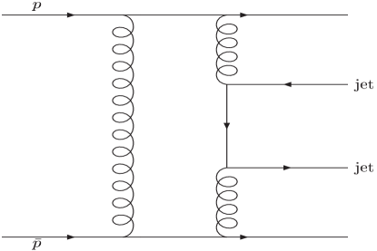
Figure 3.5: Dijet production in the non-factorised model. This model is characterised by an exclusive event topology.

A significant non-factoring contribution would manifest itself as a peak (at unity) in the distribution showing the available centre-of-mass energy which goes into the jets, known as the dijet mass or $R_{jj}$; a feature which is absent in the CDF data we consider in this thesis. However, this need not be the case for the Tevatron Run II due to higher luminosity, and this ought to be a good place to look for such evidence of a non-factorised contribution. Consequently this thesis does not consider such models.

3.3.4 Breakdown of factorisation and gap survival

The notion of a parton density in QCD is only useful if it has the property of universality. This means that once a parton density has been extracted from one process, it should be able to predict others processes with great accuracy. The current pomeron parton densities have been extracted from HERA DIS experiments, where the structure function $F_{2}^{D(3)}$ was measured. However when it came to testing HERA parton densities at the Tevatron, for hadron-hadron collisions, it was found that they overestimated the data [22, 29]. This violation of factorisation has been understood in terms of simple models, which indicate that the rapidity gaps will be filled with secondary interactions, from spectator partons in the beam. These models also indicated that the process of spoiling the gap can be approximated by a simple overall multiplicative factor $S^{2}$ [30, 32, 31, 35, 41, 42, 44], with a weak process and $\sqrt{s}$ dependence. For some processes at HERA, this factor has been estimated to be $\sim 0.6$ [45], and some Tevatron processes have been estimated to have a $S^{2}\sim 0.1$ [31, 34]. In recent times various models have been postulated for the calculation of the gap survival factor [30], and seem to support this latter figure when applied to Tevatron observables. Therefore, as this work involves using HERA parton densities at the Tevatron, we expect that factorisation will be violated and we will include in our predictions an overall gap survival factor, $S^{2}$. We will extract this factor by fitting our overall cross sections to data.

3.4 POMWIG - a Monte Carlo for Diffractive processes

The event generator POMWIG [27] is used in this work to study the hadronic diffractive process. The modifications to the HERWIG Monte Carlo event generator [16, 17] to study diffractive events are very simple once it is noticed that pomeron exchange events in hadron-hadron collisions look very much like the resolved part of photoproduction in electron/proton collisions. In the latter type of event, the electron radiates a quasi-real photon according to a flux formula. This photon is then considered to have a partonic content which interacts, through QCD processes, with the partonic content of the proton. Therefore we can study pomeron exchange events in POMWIG by replacing the photon flux with a pomeron flux and by replacing the parton density of the photon with that of the pomeron. This philosophy is illustrated in figure 3.6.

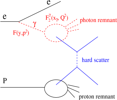
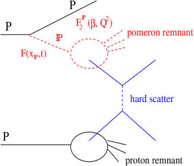
Figure 3.6: The similarity between the resolved part of photoproduction and pomeron exchange events. Figure from [27].

POMWIG is available as a modification package to HERWIG, and adopts the philosophy of minimal changes to the HERWIG structure. The generator uses the factorised IS model at the parton level, with pomeron fluxes and parton densities we will discuss later in this section, and allows the final state partons to evolve into hadrons using a parton shower and hadronisation model, as discussed in the introduction to this thesis. The inclusion of the fragmentation physics through a Monte Carlo simulation allows the phenomenological impact to be assessed.

In POMWIG, the pomeron and reggeon fluxes are parameterised as

$$f_{\mathbb{P}/p}(x_{\mathbb{P}}) = N\int_{t_{\mathrm{max}}}^{t_{\mathrm{min}}}\frac{e^{B_{\mathbb{P}}t}}{x_{\mathbb{P}}^{2\alpha_{\mathbb{P}}(t)-1}},$$

$$f_{\mathbb{R}/p}(x_{\mathbb{P}}) = \mathcal{C}_{\mathbb{R}}\int_{t_{\mathrm{max}}}^{t_{\mathrm{min}}}\frac{e^{B_{\mathbb{R}}t}}{x_{\mathbb{P}}^{2\alpha_{\mathbb{R}}(t)-1}},$$ (3.20)

where $\alpha_{\mathbb{P}}(t)=\alpha_{\mathbb{P}}(0)+\alpha^{\prime}_{\mathbb{P}}t$ and $\alpha_{\mathbb{R}}(t)=\alpha_{\mathbb{R}}(0)+\alpha^{\prime}_{\mathbb{R}}t$. The constant $N$ is chosen so that $F_{2}^{D(3)}$ matches the H1 data at $x_{\mathbb{P}}=0.003$ and similarly the constant $\mathcal{C}_{\mathbb{R}}$ is found from data. The flux parameters used are those found by the H1 collaboration, assuming there is no pomeron/reggeon interference contribution to $F_{2}^{D(3)}$. The default parameters are given in table 3.2.

Quantity	Value
$\alpha_{\mathbb{P}}$	1.20
$\alpha_{\mathbb{R}}$	0.57
$\alpha^{\prime}_{\mathbb{P}}$	0.26
$\alpha^{\prime}_{\mathbb{R}}$	0.9
$B_{\mathbb{P}}$	4.6
$B_{\mathbb{R}}$	2.0
$C_{\mathbb{R}}$	48

Table 3.2: The default POMWIG parameters.

In this work we use the H1 leading order (LO) pomeron fits to $F_{2}^{D(3)}$ measurements [28]. The measurement of $F_{2}^{D(3)}$ is quark dominated and gluon sensitivity enters only through scaling violations. Hence the gluon density has a large uncertainty of around 30% in the relevant region. This is important for the gluon dominated DPE process. The gluon densities are illustrated in figure 3.7.

Figure 3.7: The gluon densities in the pomeron as fitted by H1. The fits are evaluated at $Q^{2}=50$ GeV², the typical scale of the jet transverse energy at CDF, and are multiplied by the pomeron flux factor at $\xi_{p}=0.1$.

The mean value of $\beta$ relevant at the Tevatron is in the region of 0.3 to 0.4. Fit 4 has a gluon content that is heavily suppressed relative to fits 5 and 6 (hence fit 4 is quark-dominated), and fit 6 is peaked at high $\beta$. Fits 5 and 6 are now the favoured fits to describe H1 data [28].

POMWIG also allows us to include the effect of non-diffractive contributions through an additional Regge exchange, which we refer to as the reggeon contribution. This is expected to be important in the region of $\xi_{\bar{p}}$ explored at the Tevatron. Following H1, we estimate reggeon exchange by assuming that the reggeon can be described by the pion parton densities of Owens [46]. This contribution is added incoherently to the pomeron contribution. For further details of the implementation we refer the reader to [27].

3.5 Results

In this section we compare our results using the IS model and POMWIG with the Tevatron DPE data. We start by testing POMWIG against an independent IS calculation, which we performed by the direct integration of equation (3.19) using the H1 pomeron flux and parton density. All results using POMWIG are then shown at the parton level, at the hadron level and at the hadron level with out-of-cone corrections implemented. To assist in the interpretation of the results, we then comment on results at the parton shower level.

3.5.1 Hadronisation and parton shower effects

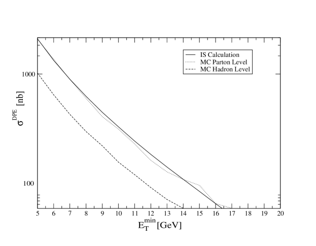
Figure 3.8: The total cross-section at both parton and hadron level, plotted as a function of the minimum transverse energy of the dijets.

Figure 3.8 demonstrates the agreement between POMWIG and an independent calculation for the total DPE cross-section as a function of the minimum jet transverse energy $E^{min}_{T}$. These curves were produced using H1 fit 5 and contain only the pomeron exchange contribution. More interestingly, we see that the curve which describes the total cross section after the effects of fragmentation (hadronisation and parton showering) have been included shows a significant reduction relative to the naive parton level calculation. This suppression effect may be understood by observing that the effect is a shift in the cross-section by $\Delta E_{T}=2$ GeV. This is a direct consequence of the broadening of the jet profile by the parton shower and hadronisation. The reduction is lower for the quark dominated fit (H1 fit 4) since quark jets tend to have a narrower profile. In practice, this hadronisation suppression will reduce the cross section by around a factor of 5.

3.5.2 Total cross section

We now turn our attention to the comparison of our theoretical predictions to the measured total cross section. The analysis we perform includes the processes in which the exchange particles are either both pomerons or both reggeons. We do not include the case where one is a reggeon and the other is a pomeron, nor do we include interference contributions. Whilst the latter may be small, the former will not be if the pure reggeon contribution is not negligible. This limitation arises since pomeron-reggeon interactions are not yet included in POMWIG. The results are presented in table 3.3 for $E_{T}^{\mathrm{min}}>7$ GeV and in table 3.4 for $E_{T}^{\mathrm{min}}>10$ GeV at $\sqrt{s}=1.8$ TeV (for the data, the first error is statistical and the second is systematic). The parton level result is found by considering the two partons produced from the hard event as final state jets, the hadron level result is found by applying the cone jet algorithm to the produced hadrons, and the out-of-cone corrections result is found by applying the CDF out-of-cone corrections to the hadron level result .

	Parton level [nb]	Hadron level [nb]	Hadron level + oc [nb]
CDF Result			43.6 $\pm$ 4.4 $\pm$ 21.6
IP fit 4	6.4	2.2	7.3
IP fit 5	859.3	190.6	661.8
IP fit 6	886.7	230.8	702.1
IR	184.7	13.2	244.1
IP+IR fit 4	191.1	15.4	251.4
IP+IR fit 5	1044.0	203.8	905.9
IP+IR fit 6	1071.4	244.0	946.2

Table 3.3: The total DPE cross-sections for a $E_{T}^{\mathrm{min}}$ cut of $7$ GeV at $\sqrt{s}=1.8$ TeV. The contributions from pomeron and reggeon exchange are shown separately.

	Parton level [nb]	Hadron level [nb]	Hadron level + oc [nb]
CDF Result			3.4 $\pm$ 1.0 $\pm$ 2.0
IP fit 4	1.2	0.4	1.4
IP fit 5	138.6	31.2	110.9
IP fit 6	174.7	42.9	141.7
IR	13.2	0	13.2
IP+IR fit 4	14.4	0.4	14.6
IP+IR fit 5	151.8	31.2	124.1
IP+IR fit 6	187.9	42.9	154.9

Table 3.4: The total DPE cross-sections for a $E_{T}^{\mathrm{min}}$ cut of 10 GeV at $\sqrt{s}=1.8$ TeV. The contributions from pomeron and reggeon exchange are shown separately.

Using fit 5, the overall cross section that we predict for a $E_{T}^{\mathrm{min}}$ cut of $7$ GeV is $203.8$ nb at the hadron level. When we apply out-of-cone corrections to this hadron level result we obtain a total cross section of $905.9$ nb; this is close to the parton level result and indicates that the out-of-cone corrections, as derived from Run I data, are approximately achieving what they were intended to do and sufficient amount of transverse energy is being added to the jets to “correct them” back to parton level. As we discussed in section 3.2, it is the out-of-cone corrected data that we need to compare to the CDF experimental data.

This (out-of-cone corrected) predicted total cross section of 905.9 nb is in excess of the experimental value of 43.6 nb. A similar excess is present with a $E_{T}^{\mathrm{min}}$ cut of $10$ GeV. However, we can match our results to the data if we assume an overall multiplicative gap survival probability of around 5%. The large reggeon contribution implies a non-negligible pomeron-reggeon contribution and naively estimating this as twice the geometric mean of the pomeron-pomeron and reggeon-reggeon contributions would push the gap survival factor down to around 3%. Given that the systematic error on the CDF cross sections is high, that the uncertainty in our knowledge of the gluon density directly affects the normalisation of the cross section, and that the size of the reggeon contribution is also uncertain it is not possible to make a more precise statement about gap survival. In any case the value we obtain agrees well with the expectations of [31, 32]. Both fits 5 and 6 can describe the data in this way, although measurements of diffractive dijet production at HERA suggest that fit 5 is favoured [47]. The ratio of the fit 5 to the fit 4 cross sections is of the order of 100, which we can understand from the ratio of the gluon densities, illustrated in figure 3.7. This ratio is 10, which becomes 100 when we consider the gluons in both pomerons. Note that the relative size of the reggeon contribution compared to the pomeron contribution is not small.

The suppression of the total cross section, relative to the naive parton level result, resulting from the parton shower phase in POMWIG has been looked at in [35]. Not surprisingly, the parton shower phase of POMWIG is responsible for a large part of the suppression relative to the naive parton level prediction.

3.5.3 Event distributions

In figures 3.9 and 3.10 we show distributions in number of events of the mean jet transverse energy, $E_{T}^{*}$, the mean jet rapidity, $\eta^{*}$, the azimuthal separation of the jets, $\Delta\phi$, and the dijet mass fraction, $R_{jj}$:

$$R_{jj}=\frac{\sum_{i}E_{i}}{\xi_{p}\xi_{\bar{p}}s}$$

$$\approx\beta_{p}\beta_{\bar{p}}.$$ (3.21)

The sum in the numerator is over all particles in the dijets. Some of these distributions have also been examined in [33]. In figure 3.9 we compare the data to results at the parton and hadron level, and we show the reggeon contribution separately. In figure 3.10 we show results at the hadron level for the three different H1 pomeron parton density functions.

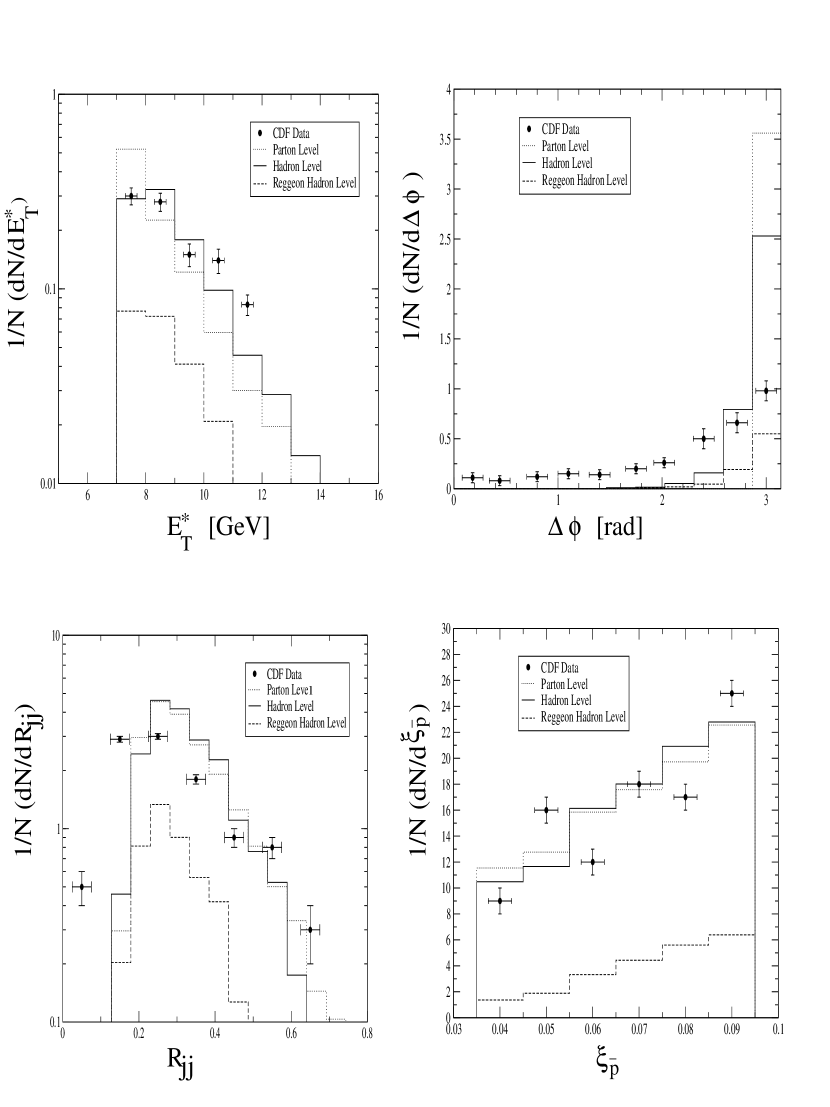
Figure 3.9: Comparison of theoretical predictions at the parton and the hadron level. Also shown is the separate contribution from the reggeon (normalised relative to the total).

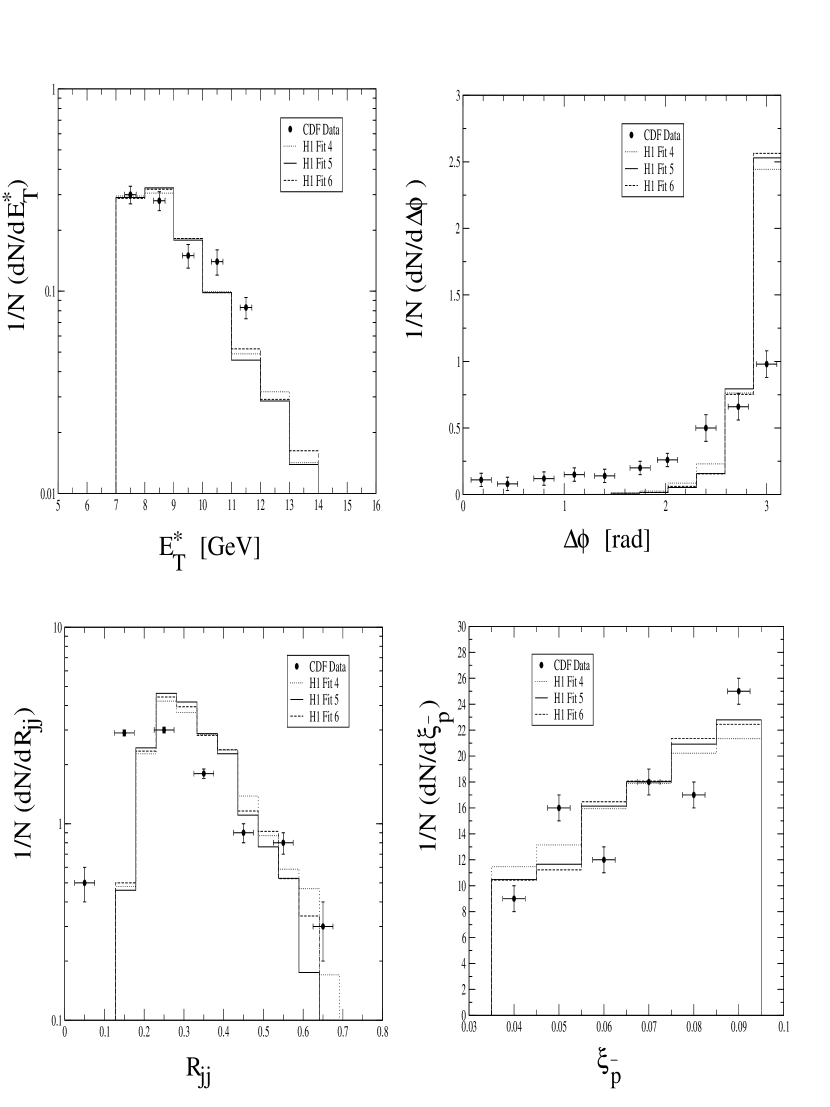
Figure 3.10: Comparison of theoretical predictions for the different H1 fits to the pomeron parton density functions at the hadron level.

We urge caution when comparing the data and theory as is done in figures 3.9 and 3.10 since the data are not corrected for detector effects. The existence of the long tail to low angles in the $\Delta\phi$ distribution illustrates the dangers: there is no possibility to produce such a long tail in a hadron level Monte Carlo simulation. This tail is caused by misidentifying the two highest $E_{T}$ jets in a three-jet event and defining $\Delta\phi$ as the azimuthal separation between two neighbouring jets; this cannot occur in a Monte Carlo simulation that has not been corrected for detector effects. Hence we are unable to draw any strong conclusions until the corrected data become available.

3.6 Conclusions

The work of this chapter has been focused on the so-called double pomeron exchange (DPE) process recently measured at the Tevatron [26]. This process is characterised by a double rapidity gap separating the intact, diffracted interacting hadrons from a central dijet system. We have extended previous calculations [22, 29] by including the effects of parton showering and hadronisation and found that they lead to a suppression of the cross-section relative to the naive parton level by a factor of around 5. We also found that, in the kinematic region probed by the Tevatron, the effect of non-diffractive (reggeon) exchange is probably important. The out-of-cone corrections used by CDF in their experimental analyses have been included in our cross section predictions and we found that, if we use a gap survival probability [30] of around 5%, we can describe the data in a natural way. At the present time the issue of gap survival, which embodies a violation of diffractive factorisation, is not very well understood. However, it is encouraging that we are able to describe the data with a gap survival probability which is consistent with previous theoretical estimates.

The Tevatron Run II has produced around 10,000 DPE events, which are in the process of being analysed. Once this has occurred, and theoretical studies like this one have been carried out, we will be in a far stronger position to understand double diffractive processes.

Finally, we can claim that one can use HERA partons at the Tevatron. When the parton level calculations of [22, 29] were carried out, the very large theory-to-experiment ratio meant that a description of the data was impossible, even with gap survival. However, a harder (and more appropriate) pomeron intercept, new parton densities in the pomeron and a gap survival factor combine to explain this excess.

Chapter 4 Resummation from factorisation

4.1 Introduction

In this survey chapter we shall discuss the factorisation of cross sections in specific regions of phase space [6]. We shall make a statement of factorisation specific to colour exchange processes in QCD [48], and develop the consequences: the resummation of the soft and the jet functions [49, 50, 52, 48, 51]. The final form of the cross section is derived, with the leading logarithms of the jet function and the next-to-leading logarithms of the soft function resummed, the latter being in terms of so-called soft anomalous dimension matrices [48, 53, 54]. The application of these techniques to rapidity gap processes is then discussed, where we are interested in soft, wide angle radiation [53] into a restricted angular region. In these applications we are interested in colour evolution and not in the resummation of the colour-diagonal jets; hence the soft logarithms become the leading logarithms. In this chapter we refer the reader to the literature for the proofs of the factorisation theorems we use [6], and our aim is a survey of the consequences of factorisation and the phenomenological applications to rapidity gap processes.

4.2 Factorisation

In this section we will describe the factorisation properties of the QCD cross sections we are interested in. The resummation formalism developed by Collins, Soper and Sterman [6, 52, 48, 7] (known as CSS) depends on the factorisation properties obeyed by a cross section, with a hard scale $Q$, in a particular limit of its final state phase space. In such regions of phase space, partons which are off-shell by order $Q^{2}$ are described by a hard scattering function $H$, and its complex conjugate $H^{*}$. On-shell particles with momenta $\sim Q$ fall into “jets” of collinear particles, which will have the interpretation of hadronic jets if they lie in the final state and as parton densities if they lie in the initial state of a hadron-initiated process. We assume that the final state of this process is in the elastic limit and all finite energy particles are concentrated in the jet functions; hence the factorisation is valid at an “edge” of phase space for a given observable. This part of phase space, where there is just enough energy to produce the final state jets and very little else, is known as the threshold region. In addition, the cross section involves the emission of soft particles, represented by a function $S$. In this work we are interested in hadron-initiated processes to jets, where it has been observed that there is no unique way of defining colour exchange in a finite amount of time. This is due to the fact that even very soft gluons carry colour and we can exchange an arbitrary number of these long-wavelength gluons in the period of time that is just after the short distance (short time) hard event. Therefore we expect the functions from which we construct the cross section to be written as matrices in the space of possible colour flows - specifically the hard and soft functions, as the jets themselves contain only collinear partons and are incoherent to the colour exchange. We can understand the need for a matrix structure by noticing that as the factorisation scale changes, gluons that are part of the hard function may need to be moved to the soft function (or vice versa), changing the colour content of both. The matrix structure of the soft function will be discussed further in section 4.7, where we discuss the construction of eikonal cross sections.

The elastic limit of the cross section is isolated by introducing an appropriate weight [7] for each final state. The weight, which is a linear function of all final state particles if it is possible to resum the observable, determines the contribution of each state to the cross section and vanishes in the elastic limit. In effect the weight parameterises the distance in phase space from the elastic limit. We shall assume that the contributions to the weight of particles in the soft function, $\omega_{s}$, and from particles in the jet functions, $\omega_{i}\,(i=1\dots n)$, are additive,

$$\omega=\sum_{i}^{n}\omega_{i}+\omega_{s},$$ (4.1)

for a $n$ jet cross section, and the corresponding statement of factorisation near the elastic limit is written as a convolution over the weights [48],

$$\sigma(\omega)=H^{(0)}_{IJ}\left(\frac{p_{i}}{\mu},\xi_{i}\right)\int \frac{\mathrm{d}\omega_{s}}{\omega_{s}}\left[\prod_{i}^{n}\frac{\mathrm{d}\omega_{i}}{\omega_{i}}\right]$$

$$\times \left[\prod_{i}^{n}J_{i}^{(0)}\left(\frac{p_{i}\cdot\xi_{i}}{\mu},\frac{\omega_{i}Q}{\mu}\right)\right]$$

$$\times S^{(0)}_{JI}\left(\frac{\omega_{s}Q}{\mu},\nu_{i},\xi_{i}\right)\delta(\omega-\sum_{i}^{n}\omega_{i}-\omega_{s}),$$ (4.2)

where we have suppressed the functional dependence on $\alpha_{s}$ and $i=1\dots n$. Note that the arguments of $H^{(0)}$ and $S^{(0)}$ depend on all possible variables with $i$ subscripts. For example, for $n=2$ we would have $H^{(0)}(p_{1}/\mu,p_{2}/\mu,\xi_{1},\xi_{2})$. This expression is our starting point and is the cross section for a hard event $H$, described by $H_{IJ}$, with $n$ light-like jets of particles, with momenta $p_{i}$. The factorisation scale is denoted $\mu$. The kinematic details are determined by the precise process under consideration; for example in $e^{+}e^{-}$ annhilation ($n=2$), each $p_{i}$ labels an outgoing jet and we define

$$Q^{2}=(p_{1}+p_{1})^{2}.$$ (4.3)

The jets are described by the functions $J_{i}$. The indices $I$ and $J$ label the colour structure of the hard scattering and each matrix has two indices - one for the amplitude and another for its complex conjugate. The vectors $\xi_{i}$ are used to define a jet in terms of a matrix element (just like a gauge-fixing vector) and hence are arbitrary, and the vectors $\nu_{i}$ define the direction of the appropriate jet. The function $S_{JI}$ describes the dynamics of partons with energy less than the soft scale $\omega_{s}Q$; we will consider its construction later in the chapter but it is enough to say that the soft dynamics of this function exactly match those of the full theory. Hence resummation of the soft function is equivalent to the resummation of the soft dynamics of the full cross section. We have denoted bare, unrenormalised quantities by a $(0)$ superscript, and deal with the issue of renormalisation in section 4.3. The proof of the factorisation statement follows standard proofs of factorisation [6], and shall not be discussed in this thesis. In this chapter we are interested in the consequences of factorisation, and so will consider a simplified cross section with only 1 jet. Therefore $Q^{2}=p^{2}$ and we write

$$\sigma(\omega)=H^{(0)}_{IJ}\left(\frac{p}{\mu},\xi\right)\int\frac{\mathrm{d}\omega_{J}}{\omega_{J}}\frac{\mathrm{d}\omega_{s}}{\omega_{s}}J^{(0)}\left(\frac{p\cdot\xi}{\mu},\frac{\omega_{J}Q}{\mu}\right)S^{(0)}_{JI}\left(\frac{\omega_{s}Q}{\mu},\nu,\xi\right)\delta(\omega-\omega_{J}-\omega_{s}),$$ (4.4)

where we have suppressed the functional dependence on $\alpha_{s}$. The convolution in weight unravels after the transformation,

$$\sigma(N)=\int_{0}^{\infty}d\omega e^{-N\omega}\sigma(\omega),$$ (4.5)

where the moment variable $N$ is conjugate to $\omega$, and the leading behaviour in the small $\omega$ limit is determined by the large $N$ behaviour. We therefore obtain, in moment space,

$$\sigma(N)=H^{(0)}_{IJ}\left(\frac{p}{\mu},\xi\right)\tilde{J}^{(0)}\left(\frac{p\cdot\xi}{\mu},\frac{Q}{N\mu}\right)\tilde{S}^{(0)}_{JI}\left(\frac{Q}{N\mu},\nu,\xi\right),$$ (4.6)

where we define the transform of the soft function by

$$\tilde{S}^{(0)}_{JI}\left(\frac{Q}{N\mu},\nu,\xi\right)=\int_{0}^{\infty}\frac{d\omega_{s}}{\omega_{s}}e^{-N\omega_{s}}S^{(0)}_{JI}\left(\frac{\omega_{s}Q}{\mu},\nu,\xi\right),$$ (4.7)

with a similar definition for the transform of the jet function. Noting the kinematical relation $p^{\mu}=Q\nu^{\mu}$ and writing the soft scale as $Q/N=Q_{s}$ we arrive at

$$\sigma(N)=H^{(0)}_{IJ}\left(\frac{Q}{\mu},\nu\cdot\xi\right)\tilde{J}^{(0)}\left(\frac{Q\nu\cdot\xi}{\mu},\frac{Q_{s}}{\mu}\right)\tilde{S}^{(0)}_{JI}\left(\frac{Q_{s}}{\mu},\nu\cdot\xi\right),$$ (4.8)

where we have slightly changed the notation. Equation (4.8) is our statement of factorisation, in moment space, for a schematic 1 jet cross section.

4.3 Renormalisation group properties

In this section we demonstrate the renormalisation of the contributing functions [49, 50, 48, 7] appearing in the factorised cross section. We start from the factorised expression discussed in the last section, written with $n$ jets and in matrix notation,

$$\sigma=\mathrm{Tr}(\uuline{H}^{(0)}\,\uuline{S}^{(0)})\prod_{i}^{n}J_{i}^{(0)},$$ (4.9)

in terms of the bare quantities. For the remaining part of this chapter, we shall drop the “tilde” notation for quantities in moment space; it will be clear from the context what is meant. We assume that $J_{i}$ renormalises multiplicatively

$$J_{i}^{(0)}=Z_{i}(\mu)J_{i}(\mu)$$ (4.10)

where $Z_{i}(\mu)$ is an UV renormalisation constant, $J_{i}(\mu)$ is the finite (renormalised) jet function and $\mu$ is an arbitrary renormalisation scale (different to the factorisation scale used in the last section). By observing that the bare jet function must be independent of the renormalisation scale,

$$\mu\frac{\partial}{\partial\mu}J_{i}^{(0)}=0,$$ (4.11)

we arrive at the renormalisation group equation for $J_{i}$,

$$\mu\frac{\partial}{\partial\mu}J_{i} = -Z_{1}^{-1}\left(\mu\frac{\partial}{\partial\mu}Z_{i}\right)J_{i},$$ (4.12)

$$= -\gamma_{i}J_{i}.$$ (4.13)

In the last equality we have defined the (so called) jet anomalous dimension.

The renormalisation of $\uuline{S}$ comes from the UV limit of the virtual corrections. We assume that the amplitude and its complex conjugate renormalise multiplicatively,

$$\uuline{S}^{(0)}=\uuline{Z_{s}}(\mu)^{\dagger}\,\uuline{S}(\mu)\,\uuline{Z_{s}}(\mu).$$ (4.14)

Again, $\uuline{Z_{s}}$ is a UV renormalisation constant, $\uuline{S}$ is the finite (renormalised) soft function and $\mu$ is an arbitrary renormalisation scale. Exploiting the invariance of the bare soft function against changes in $\mu$,

$$\mu\frac{\partial}{\partial\mu}\uuline{S}^{(0)}=0,$$ (4.15)

means we arrive at the RGE for the soft function

$$\mu\frac{\partial}{\partial\mu}\uuline{S} = -\left[\uuline{Z_{s}}^{-1\,\dagger}\left(\mu\frac{\partial}{\partial\mu}\uuline{Z_{s}}^{\dagger}\right)\right]\uuline{S}-\uuline{S}\left[\left(\mu\frac{\partial}{\partial\mu}\uuline{Z_{s}}\right)\uuline{Z_{s}}^{-1}\right],$$ (4.16)

$$= -\uuline{\Gamma_{s}}^{\dagger}\,\uuline{S}-\uuline{S}\,\uuline{\Gamma_{s}}.$$ (4.17)

In the last equality we have defined the soft anomalous dimensions. The scale-independence of $\sigma$ now allows us to derive the renormalisation properties of $\uuline{H}$. Inserting the renormalised expressions for the bare soft and jet functions into the factorised expression for the cross section gives

$$\sigma = \mathrm{Tr}\left(\uuline{H}^{(0)}\uuline{Z_{s}}^{\dagger}\,\uuline{S}\uuline{Z_{s}}\right)\prod_{i}Z_{i}J_{i},$$ (4.18)

$$= \mathrm{Tr}(\uuline{H}\,\uuline{S})\prod_{i}J_{i},$$ (4.19)

which implies that $\uuline{H}^{(0)}$ renormalises multiplicatively,

$$\uuline{H}^{(0)}=\prod_{i}Z_{i}^{-1}\uuline{Z_{s}}^{-1}\,\uuline{H}\,\uuline{Z_{s}}^{-1\,\dagger}.$$ (4.20)

We can now write down the hard RGE,

$$\mu\frac{\partial}{\partial\mu}\uuline{H}=\sum_{i}\gamma_{i}\uuline{H}+\Gamma_{s}\uuline{H}+\uuline{H}\uuline{\Gamma_{s}}^{\dagger},$$ (4.21)

by noting that the bare hard function is renormalisation scale independent.

The discussion so far has been for an observable in the threshold region of its final state phase space, where there is no extra energy available for gluon emission. This restriction that the gluon emission must be very soft means that this factorisation is also valid for rapidity gap observables. In such cross sections the gluon emission into a measured gap region is restricted, whilst being fully inclusive elsewhere, so the soft function depends on radiation into the gap $\Omega$, at scale $Q_{s}$. To be more general, the soft function also depends on radiation out of the gap, the region $\bar{\Omega}$, at scale $M$. Therefore we can write $\uuline{S}=\uuline{S}(Q_{s}/\mu,M/\mu)$ and trade the $\mu$ derivative for $Q_{s}$ and $M$ derivatives to obtain

$$\left(Q_{s}\frac{\partial}{\partial Q_{s}}-\beta(g_{s})\frac{\partial}{\partial g_{s}}\right)\uuline{S}=-\uuline{\Gamma_{s}}^{\dagger}\,\uuline{S}-\uuline{S}\,\uuline{\Gamma_{s}}-M\frac{\partial}{\partial M}\uuline{S}.$$ (4.22)

In [55] the $M$ derivative has been interpreted to produce non-global logarithmic enhancements in $\uuline{S}$, starting at $\alpha_{s}^{2}\log^{2}(Q_{s})$. Configurations producing these logarithmically enhanced terms arise from radiation being emitted into $\Omega$ from secondary gluons in $\bar{\Omega}$ and as a result resolve the colour structure of the secondary gluon. Therefore such contributions cannot be absorbed in an anomalous dimension matrix for $2\rightarrow 2$ scattering in a simple way, and we drop such non-global terms from our soft RGE. We will include such effects (non-global logarithms) in a new way in chapter 5. Therefore our soft RGE (correct to primary leading log level) is

$$\left(Q_{s}\frac{\partial}{\partial Q_{s}}-\beta(g_{s})\frac{\partial}{\partial g_{s}}\right)\uuline{S}=-\uuline{\Gamma_{s}}^{\dagger}\,\uuline{S}-\uuline{S}\,\uuline{\Gamma_{s}}.$$ (4.23)

We will solve the soft and jet function RGEs in the next section.

4.4 Resummation

In this section we discuss how to use the factorised expression to produce resummed expressions for the various contributing functions in the cross section. The resummation of the jet and soft functions parallels that of [48].

4.4.1 Resummation of the jet functions

The expression for the factorised 1 jet cross section (in moment space), introduced in section 4.2, is

$$\sigma(Q,Q_{s},\alpha_{s})=H_{IJ}\left(\frac{Q}{\mu},\nu\cdot\xi,\alpha_{s}(\mu)\right)J\left(\frac{Q\nu\cdot\xi}{\mu},\frac{Q_{s}}{\mu},\alpha_{s}(\mu)\right)S_{JI}\left(\frac{Q_{s}}{\mu},\nu\cdot\xi,\alpha_{s}(\mu)\right).$$ (4.24)

In this equation, we have restored the $\alpha_{s}$ dependence of all the contributing functions. We will now define the scaled gauge parameters, $r$, such that

$$r=\nu\cdot\xi\Rightarrow p\cdot\xi=Qr.$$ (4.25)

This factorisation cannot depend on the exact choice of the quantity $r$,

$$r\frac{\partial}{\partial r}\sigma(Q,Q_{s},\alpha_{s})=0,$$ (4.26)

and any changes in the function $J$ must be compensated by changes in the functions $S$ and $H$. Therefore (suppressing function arguments)

$$\mathrm{Tr}\{\uuline{H}\,\uuline{S}\}J^{-1}r\frac{\partial}{\partial r}J=-\mathrm{Tr}\left\{(r\frac{\partial}{\partial r}\uuline{H})\uuline{S}\right\}-\mathrm{Tr}\left\{\uuline{H}(r\frac{\partial}{\partial r}\uuline{S})\right\}.$$ (4.27)

If we assume that this equation is true element-by-element,

$$\uuline{H}\,\uuline{S}J^{-1}r\frac{\partial}{\partial r}J=-(r\frac{\partial}{\partial r}\uuline{H})\uuline{S}-\uuline{H}(r\frac{\partial}{\partial r}\uuline{S}),$$ (4.28)

we obtain (restoring the function arguments)

$$\uuline{\mathbbm{1}}J^{-1}r\frac{\partial}{\partial r}J\left(\frac{Qr}{\mu},\frac{Q_{s}}{\mu},\alpha_{s}(\mu)\right) = -\uuline{H}^{-1}r\frac{\partial}{\partial r}\uuline{H}\left(\frac{Q}{\mu},r,\alpha_{s}(\mu)\right)$$ (4.29)

$$- \left(r\frac{\partial}{\partial r}\uuline{S}\left(\frac{Q_{s}}{\mu},r,\alpha_{s}(\mu)\right)\right)\uuline{S}^{-1}.$$

The log-derivative of $J$ may depend on the hard scale $Q$ or the soft scale $Q_{s}$. This variation can be split into two functions: one function which depends on the variables held in common by $J$ and $\uuline{H}$, namely $Qr/\mu$ and $\alpha_{s}(\mu)$, and one function which depends on the variables held in common by $J$ and $\uuline{S}$, namely $Q_{s}/\mu$ and $\alpha_{s}(\mu)$. Therefore we can write

$$\uuline{\mathbbm{1}}J^{-1}r\frac{\partial}{\partial r}J(\frac{Qr}{\mu},\frac{Q_{s}}{\mu},\alpha_{s}(\mu))=G\left(\frac{Qr}{\mu},\alpha_{s}(\mu)\right)\uuline{\mathbbm{1}}+K\left(\frac{Q_{s}}{\mu},\alpha_{s}(\mu)\right)\uuline{\mathbbm{1}},$$ (4.30)

where we define

$$\uuline{H}^{-1}r\frac{\partial}{\partial r}\uuline{H}\left(\frac{Q}{\mu},r,\alpha_{s}(\mu)\right) = -G\left(\frac{Qr}{\mu},\alpha_{s}(\mu)\right)\uuline{\mathbbm{1}},$$ (4.31)

$$\left(r\frac{\partial}{\partial r}\uuline{S}\left(\frac{Q_{s}}{\mu},r,\alpha_{s}(\mu)\right)\right)\uuline{S}^{-1} = -K\left(\frac{Q_{s}}{\mu},\alpha_{s}(\mu)\right)\uuline{\mathbbm{1}}.$$ (4.32)

The auxiliary function $G$ depends on the hard scale $Q$ and contains all the short-distance physics; conversely the function $K$ depends on the soft scale $Q_{s}$ and contains all the long-distance physics. Both of these functions depend on the gauge parameter $r$. Applying the RG-invariance operator $\mu\partial_{\mu}$ to this equation, swapping the order of the differential operators, using the RGE of $J$ and noting that $\gamma_{J}$ is $r$ independent implies that the combination $G+K$ is RG-invariant,

$$\mu\frac{\partial}{\partial\mu}\left[G\left(\frac{Qr}{\mu},\alpha_{s}(\mu)\right)+K\left(\frac{Q_{s}}{\mu},\alpha_{s}(\mu)\right)\right]=0.$$ (4.33)

Separating variables we obtain

$$\mu\frac{\partial}{\partial\mu}G\left(\frac{Qr}{\mu},\alpha_{s}(\mu)\right) = +\gamma_{K}(\alpha_{s}(\mu)),$$ (4.34)

$$\mu\frac{\partial}{\partial\mu}K\left(\frac{Q_{s}}{\mu},\alpha_{s}(\mu)\right) = -\gamma_{K}(\alpha_{s}(\mu)),$$ (4.35)

where the separation constants (Sudakov anomalous dimensions) only depend on the common variable $\alpha_{s}(\mu)$. To solve these equations, we postulate the solution (which can be checked by differentiating)

$$K\left(\frac{Q_{s}}{\mu},\alpha_{s}(\mu)\right)=K(\quad)+\int_{\mu}\frac{d\mu^{\prime}}{\mu^{\prime}}\gamma_{K}(\alpha_{s}(\mu^{\prime})).$$ (4.36)

Now we set the upper limit of the integral to the scale $Q_{s}$ and choose the constant $K(\quad)$ (which denotes a $\mu$-independent $K$) to satisfy the RG equation. Doing this we obtain

$$K\left(\frac{Q_{s}}{\mu},\alpha_{s}(\mu)\right) = K(1,\alpha_{s}(Q_{s}))+\int_{\mu}^{Q_{s}}\frac{d\mu^{\prime}}{\mu^{\prime}}\gamma_{K}(\alpha_{s}(\mu^{\prime})),$$ (4.37)

$$G\left(\frac{Qr}{\mu},\alpha_{s}(\mu)\right) = G(1,\alpha_{s}(Qr))+\int_{Qr}^{\mu}\frac{d\mu^{\prime}}{\mu^{\prime}}\gamma_{K}(\alpha_{s}(\mu^{\prime})).$$ (4.38)

In order to combine these two expressions, we shift the evaluation on the coupling in equation (4.37) from $Q_{s}$ to $Qr$,

$$K(1,\alpha_{s}(Qr)) = K(1,\alpha_{s}(Q_{s}))+\int_{\alpha_{s}(Q_{s})}^{\alpha_{s}(Qr)}d\alpha_{s}\frac{\partial K(1,\alpha_{s})}{\partial\alpha_{s}},$$ (4.39)

$$= K(1,\alpha_{s}(Q_{s}))+\int_{Q_{s}}^{Qr}\frac{d\mu^{\prime}}{\mu^{\prime}}\beta(\alpha_{s}(\mu^{\prime}))\frac{\partial K(1,\alpha_{s})}{\partial\alpha_{s}}.$$ (4.40)

We have used the QCD $\beta$-function in the last line,

$$\alpha_{s}=\alpha_{s}(\mu^{\prime})\Rightarrow\mathrm{d}\alpha_{s}=\beta(\alpha_{s})\frac{\mathrm{d}\mu^{\prime}}{\mu^{\prime}},$$ (4.41)

where $\beta(\alpha_{s})=\mu^{\prime}\partial\alpha_{s}/\partial\mu^{\prime}$. Combining the $K$ and $G$ functions, we now obtain

$$G\left(\frac{Qr}{\mu},\alpha_{s}(\mu)\right) + K\left(\frac{Q_{s}}{\mu},\alpha_{s}(\mu)\right)=G(1,\alpha_{s}(Qr))+K(1,\alpha_{s}(Qr))$$ (4.42)

$$- \int_{Q_{s}}^{Qr}\frac{d\mu^{\prime}}{\mu^{\prime}}\left(\gamma_{K}(\alpha_{s}(\mu^{\prime}))+\beta(\alpha_{s}(\mu^{\prime}))\frac{\partial K(1,\alpha_{s})}{\partial\alpha_{s}}\right).$$ (4.43)

This expression can be written in the compact form

$$G\left(\frac{Qr}{\mu},\alpha_{s}(\mu)\right)+K\left(\frac{Q_{s}}{\mu},\alpha_{s}(\mu)\right)=-\int_{Q_{s}}^{Qr}\frac{d\mu^{\prime}}{\mu^{\prime}}A(\alpha_{s}(\mu^{\prime}))-A^{\prime}(\alpha_{s}(Qr)),$$ (4.44)

where we define

$$A(\alpha_{s}) = \gamma_{K}(\alpha_{s})+\beta(\alpha_{s})\frac{\partial K(1,\alpha_{s})}{\partial\alpha_{s}},$$ (4.45)

$$A^{\prime}(\alpha_{s}) = G(1,\alpha_{s})+K(1,\alpha_{s}).$$ (4.46)

We now have two evolution equations for $J$, from RG invariance and the invariance of $J$ against changes in the gauge parameters $r$,

$$\mu\frac{\partial}{\partial\mu}\log J\left(\frac{Qr}{\mu},\frac{Q_{s}}{\mu},\alpha_{s}(\mu)\right) = -\gamma_{J}(\alpha_{s}(\mu)),$$ (4.47)

$$r\frac{\partial}{\partial r}\log J\left(\frac{Qr}{\mu},\frac{Q_{s}}{\mu},\alpha_{s}(\mu)\right) = G\left(\frac{Qr}{\mu},\alpha_{s}(\mu)\right)+K\left(\frac{Q_{s}}{\mu},\alpha_{s}(\mu)\right).$$ (4.48)

The first of these two equations has the solution

$$\log J\left(\frac{Qr}{\mu},\frac{Q_{s}}{\mu},\alpha_{s}(\mu)\right)=\log J\left(\frac{Qr}{Q_{s}},1,\alpha_{s}(Q_{s})\right)-\int_{Q_{s}}^{\mu}\frac{d\mu^{\prime}}{\mu^{\prime}}\gamma_{J}(\alpha_{s}(\mu^{\prime})),$$ (4.49)

which must also obey the second equation. This gives

$$r\frac{\partial}{\partial r}\log J\left(\frac{Qr}{Q_{s}},1,\alpha_{s}(Q_{s})\right)=G\left(\frac{Qr}{Q_{s}},\alpha_{s}(Q_{s})\right)+K\left(1,\alpha_{s}(Q_{s})\right),$$ (4.50)

which has the solution (recall that both $G$ and $K$ depend on the gauge parameter $r$)

$$\log J\left(\frac{Qr}{Q_{s}},1,\alpha_{s}(Q_{s})\right) = \log J\left(1,1,\alpha_{s}(Q_{s})\right)$$ (4.51)

$$+ \int_{Q_{s}/Q}^{r}\frac{dr^{\prime}}{r^{\prime}}\left[G\left(\frac{Qr^{\prime}}{\mu},\alpha_{s}(\mu)\right)+K(1,\alpha_{s}(Q_{s}))\right]$$ (4.52)

$$= \log J\left(1,1,\alpha_{s}(Q_{s})\right)$$ (4.53)

$$+ \int_{Q_{s}/Q}^{r}\frac{dr^{\prime}}{r^{\prime}}\left[-\int_{Q_{s}}^{Qr^{\prime}}\frac{d\xi}{\xi}A(\alpha_{s}(\xi))-A^{\prime}(\alpha_{s}(Qr^{\prime}))\right],$$ (4.54)

or, after a change of variable ($r^{\prime}=\mu^{\prime}/Q$),

$$\log J\left(\frac{Qr}{Q_{s}},1,\alpha_{s}(Q_{s})\right) = \log J\left(1,1,\alpha_{s}(Q_{s})\right)$$ (4.55)

$$+ \int_{Q_{s}}^{Qr}\frac{d\mu^{\prime}}{\mu^{\prime}}\left[-\int_{Q_{s}}^{\mu^{\prime}}\frac{d\xi}{\xi}A(\alpha_{s}(\xi))-A^{\prime}(\alpha_{s}(\mu^{\prime}))\right].$$ (4.56)

Now we can write down an expression for $J$ which organises both the $Qr$ dependence and the $N$ dependence (through $Q_{s}$),

$$\log J\left(\frac{Qr}{\mu},\frac{Q_{s}}{\mu},\alpha_{s}(\mu)\right) = \log J\left(1,1,\alpha_{s}(Q_{s})\right)-\int_{Q_{s}}^{\mu}\frac{d\mu^{\prime}}{\mu^{\prime}}\gamma_{J}(\alpha_{s}(\mu^{\prime}))$$ (4.57)

$$- \int_{Q_{s}}^{Qr}\frac{d\lambda}{\lambda}\left\{\left[\int_{Q_{s}}^{\lambda}\frac{d\xi}{\xi}A(\alpha_{s}(\xi))\right]+A^{\prime}(\alpha_{s}(\lambda))\right\}.$$

Extending the $\xi$ integration range using the $\Theta$-function,

$$I=\int_{Q_{s}}^{Qr}\frac{d\xi}{\xi}A(\alpha_{s}(\xi))\Theta(\lambda-\xi),$$ (4.58)

allows us to switch the order of the $\xi$ and $\lambda$ integrals, and obtain

$$\int_{Q_{s}}^{Qr}\frac{d\xi}{\xi}A(\alpha_{s}(\xi))\int_{\xi}^{Qr}\frac{d\lambda}{\lambda}=\int_{Q_{s}}^{Qr}\frac{d\xi}{\xi}A(\alpha_{s}(\xi))\log\left(\frac{Qr}{\xi}\right).$$ (4.59)

Therefore we obtain our final form of the resummed expression for $J$, or in general for the $i^{th}$ jet, of

$$\log J_{i}\left(\frac{Qr}{\mu},\frac{Q_{s}}{\mu},\alpha_{s}(\mu)\right) = \log J_{i}\left(1,1,\alpha_{s}(Q_{s})\right)$$

$$- \int_{Q_{s}}^{\mu}\frac{d\lambda}{\lambda}\gamma_{i}(\alpha_{s}(\lambda))$$

$$- \int_{Q_{s}}^{Qr}\frac{d\xi}{\xi}\left\{A(\alpha_{s}(\xi))\log\left(\frac{Qr}{\xi}\right)+A^{\prime}(\alpha_{s}(\xi))\right\}.$$

This can be generalised to an arbitrary number of jets by repeating the reasoning for each jet. Doing so we obtain

$$\prod_{i}J_{i}\left(\frac{Qr_{i}}{\mu},\frac{Q_{s}}{\mu},\alpha_{s}(\mu)\right)=\prod_{i}J_{i}\left(1,1,\alpha_{s}(Q_{s})\right)e^{-\mathcal{S}_{J_{i}}},$$ (4.61)

where we define the jet Sudakov exponent by

$$\mathcal{S}_{J_{i}}=\int_{Q_{s}}^{\mu}\frac{d\lambda}{\lambda}\left(\gamma_{i}(\alpha_{s}(\lambda))\right)+\int_{Q_{s}}^{Qr}\frac{d\xi}{\xi}\left\{A(\alpha_{s}(\xi))\log\left(\frac{Qr}{\xi}\right)+A^{\prime}(\alpha_{s}(\xi))\right\}.$$ (4.62)

The resummation is controlled by the exponents $A$,$A^{\prime}$ and the set $\gamma_{i}$. The latter are known as anomalous dimensions, which are expressed as series in $\alpha_{s}$. This completes the resummation, in moment space, of the jet function.

4.4.2 Resummation of the soft function

The RGE for the soft function at scale $\mu$ is (suppressing $\alpha_{s}$ dependence)

$$\mu\frac{\partial}{\partial\mu}\uuline{S}(\mu)=-\uuline{\Gamma_{s}^{\dagger}}\,\uuline{S}(\mu)-\uuline{S}(\mu)\,\uuline{\Gamma_{s}}.$$ (4.63)

To solve this equation, we need to use the path-ordered exponential, which allows us to expand exponentials of non-commuting objects (in this case the non-commuting objects are matrices)

$$\mathrm{P}\exp\left(\int_{\mu}^{\mu_{0}}\frac{d\mu^{\prime}}{\mu^{\prime}}\uuline{\Gamma_{s}}(\mu^{\prime})\right) = \mathbbm{1}+\int_{\mu}^{\mu_{0}}\frac{d\mu_{1}}{\mu_{1}}\uuline{\Gamma_{s}}(\mu_{1})+\int_{\mu}^{\mu_{0}}\frac{d\mu_{1}}{\mu_{1}}\int_{\mu_{1}}^{\mu_{0}}\frac{d\mu_{2}}{\mu_{2}}\uuline{\Gamma_{s}}(\mu_{2})\uuline{\Gamma_{s}}(\mu_{1})$$ (4.64)

$$+ \dots\,\,\,+$$

$$+ \int_{\mu}^{\mu_{0}}\frac{d\mu_{1}}{\mu_{1}}\dots\int_{\mu_{n-1}}^{\mu_{0}}\frac{d\mu_{n}}{\mu_{n}}\uuline{\Gamma_{s}}(\mu_{n})\dots\uuline{\Gamma_{s}}(\mu_{1}).$$

We have introduced a new scale $\mu_{0}$ ($<\mu$). In this definition of the path-ordered exponential, we arrange the matrices in order of increasing scale from left to right (increasing $\mu$). Therefore at a new order of the expansion, we gain a new inner integration of a new variable $\mu_{n}$, from $\mu_{n-1}$ to $\mu_{0}$, and place the new $\uuline{\Gamma_{s}}(\mu_{n})$ on the left of the existing matrices. The anti-path ordered exponential, denoted $\bar{\mathrm{P}}$, is similar, except that we arrange the matrices in reverse order,

$$\bar{\mathrm{P}}\exp\left(\int_{\mu}^{\mu_{0}}\frac{d\mu^{\prime}}{\mu^{\prime}}\uuline{\Gamma_{s}^{\dagger}}(\mu^{\prime})\right) = \mathbbm{1}+\int_{\mu}^{\mu_{0}}\frac{d\mu_{1}}{\mu_{1}}\uuline{\Gamma_{s}^{\dagger}}(\mu_{1})+\int_{\mu}^{\mu_{0}}\frac{d\mu_{1}}{\mu_{1}}\int_{\mu_{1}}^{\mu_{0}}\frac{d\mu_{2}}{\mu_{2}}\uuline{\Gamma_{s}}^{\dagger}(\mu_{1})\uuline{\Gamma_{s}}^{\dagger}(\mu_{2})$$ (4.65)

$$+ \dots\,\,\,+$$

$$+ \int_{\mu}^{\mu_{0}}\frac{d\mu_{1}}{\mu_{1}}\dots\int_{\mu_{n-1}}^{\mu_{0}}\frac{d\mu_{n}}{\mu_{n}}\uuline{\Gamma_{s}}^{\dagger}(\mu_{1})\dots\uuline{\Gamma_{s}}^{\dagger}(\mu_{n}).$$

The effect of applying $\mu\partial_{\mu}$ to a path-ordered object can be seen by inspection to be

$$\mu\partial_{\mu}\mathrm{P}\exp\left(\int_{\mu}^{\mu_{0}}\frac{d\mu^{\prime}}{\mu^{\prime}}\uuline{\Gamma_{s}}(\mu^{\prime})\right) = -\mathrm{P}\exp\left(\int_{\mu}^{\mu_{0}}\frac{d\mu^{\prime}}{\mu^{\prime}}\uuline{\Gamma_{s}}(\mu^{\prime})\right)\uuline{\Gamma_{s}}(\mu),$$

$$\mu\partial_{\mu}\bar{\mathrm{P}}\exp\left(\int_{\mu}^{\mu_{0}}\frac{d\mu^{\prime}}{\mu^{\prime}}\uuline{\Gamma_{s}^{\dagger}}(\mu^{\prime})\right) = -\uuline{\Gamma_{s}^{\dagger}}(\mu)\bar{\mathrm{P}}\exp\left(\int_{\mu}^{\mu_{0}}\frac{d\mu^{\prime}}{\mu^{\prime}}\uuline{\Gamma_{s}}^{\dagger}(\mu^{\prime})\right).$$ (4.66)

Therefore it is easy to see that we can solve the soft RGE by

$$\uuline{S}(\mu)=\bar{\mathrm{P}}\exp\left(\int_{\mu}^{\mu_{0}}\frac{d\mu^{\prime}}{\mu^{\prime}}\uuline{\Gamma_{s}^{\dagger}}(\mu^{\prime})\right)\uuline{S}(\mu_{0})\mathrm{P}\exp\left(\int_{\mu}^{\mu_{0}}\frac{d\mu^{\prime}}{\mu^{\prime}}\uuline{\Gamma_{s}}(\mu^{\prime})\right).$$ (4.67)

We have picked the scale of $\uuline{S}$ on the right-hand side so that the equation is true when $\mu=\mu_{0}$. Note that if $\Gamma_{s}(\mu)$ commutes with $\Gamma_{s}(\mu^{\prime})$ the path-ordering becomes irrelevant and we recover the usual exponential form. For the soft function defined in this chapter, $\uuline{S}$ is a function of the soft scale ratio $Q_{s}/\mu$, and so the RGE is given by

$$\mu\frac{\partial}{\partial\mu}\uuline{S}\left(\frac{Q_{s}}{\mu}\right)=-\uuline{\Gamma_{s}^{\dagger}}\,\uuline{S}\left(\frac{Q_{s}}{\mu}\right)-\uuline{S}\left(\frac{Q_{s}}{\mu}\right)\,\uuline{\Gamma_{s}}.$$ (4.68)

This equation is solved by

$$\uuline{S}\left(\frac{Q_{s}}{\mu}\right)=\bar{\mathrm{P}}\exp\left(\int_{\mu}^{Q_{s}}\frac{d\mu^{\prime}}{\mu^{\prime}}\uuline{\Gamma_{s}^{\dagger}}(\mu^{\prime})\right)\uuline{S}(1)\mathrm{P}\exp\left(\int_{\mu}^{Q_{s}}\frac{d\mu^{\prime}}{\mu^{\prime}}\uuline{\Gamma_{s}}(\mu^{\prime})\right),$$ (4.69)

where we have picked the arbitrary scale $\mu_{0}=Q_{s}$.

4.4.3 The resummed expression

We can now present (in matrix notation) the resummed cross section in moment space for our 1 jet cross section. We have chosen $\mu=Q$ throughout, and so the hard function becomes $\uuline{H}(Q/\mu)\rightarrow\uuline{H}(1)$ and the integrals in the path ordered exponentials of the soft function and the jet Sudakov exponent are now between $Q$ and $Q_{s}$. We have made the choice of $r=1$ for the gauge parameter. We obtain

$$\sigma(Q,Q_{s},\alpha_{s})=\mathrm{Tr}\left\{\uuline{H}(1)\bar{\mathrm{P}}\exp\left(\int_{Q}^{Q_{s}}\frac{d\lambda}{\lambda}\uuline{\Gamma_{s}^{\dagger}}(\lambda)\right)\uuline{S}(1)\exp\left(\int_{Q}^{Q_{s}}\frac{d\lambda}{\lambda}\uuline{\Gamma_{s}}(\lambda)\right)\right\}J\left(1,\frac{Q_{s}}{Q}\right),$$ (4.70)

where we have not written the full expression for the resummed jet function, which can be read off from equation (4.61).

4.5 Diagonalisation

In this section we develop the solution, equation (4.69), of the soft RGE. We do this by choosing a basis in which the $\uuline{\Gamma_{s}}$ matrices are diagonal [53, 55], and hence are given by the eigenvalues of the matrix $\uuline{\Gamma_{s}}$,

$$\left(\tilde{\Gamma}_{s}\right)_{\gamma\beta}=\lambda^{(\beta)}\delta_{\gamma\beta},$$ (4.71)

where $\lambda_{\beta}$ denotes the eigenvalues of $\uuline{\Gamma_{s}}$. We will denote quantities in the diagonal basis with tildes. If $\uline{e}^{(J)}$ is the $J^{\mathrm{th}}$ eigenvector of $\uuline{\Gamma_{s}}$ (with eigenvalue $\lambda^{(J)}$) then the matrix whose columns are the eigenvectors,

$$R_{IJ}=e_{I}^{(J)},$$ (4.72)

will diagonalise $\uuline{\Gamma_{s}}$. We therefore write the anomalous dimension matrices in the new diagonal basis using a similarity transform,

$$\left(\tilde{\Gamma_{s}}(\Delta\eta,\Omega)\right)_{\gamma\beta}=\lambda^{(\beta)}\delta_{\gamma\beta}=R^{-1}_{\gamma I}\left(\Gamma_{s}(\Delta\eta,\Omega)\right)_{IJ}R_{J\beta}.$$ (4.73)

To do this we need to explicitly expand the anomalous dimension matrices to one-loop (work at leading order in $\alpha_{s}$),

$$\uuline{\Gamma_{s}}(\lambda)=\frac{\alpha_{s}(\lambda)}{\pi}\uuline{G}.$$ (4.74)

where $\uuline{G}$ is a constant (i.e. scale independent) matrix. This implies that different scales will commute with each other (all scales have the same constant matrix $\uuline{G}$) inside of the path-ordering, and the matrix can come outside of the integral on the left hand side. Hence

$$\mathrm{P}\exp\left(\int_{Q}^{Q_{s}}\frac{d\lambda}{\lambda}\uuline{\Gamma_{s}}(\lambda)\right)=\exp\left(\uuline{G}\int_{Q}^{Q_{s}}\frac{d\lambda}{\lambda}\frac{\alpha_{s}(\lambda)}{\pi}\right).$$ (4.75)

Now by inserting $\uuline{R}\,\uuline{R}^{-1}=\uuline{I}$ as required, we rewrite the path-ordered exponential as

$$\left(\uuline{R}^{-1}\mathrm{P}\exp\left(\int_{Q}^{Q_{s}}\frac{d\lambda}{\lambda}\uuline{\Gamma_{s}}(\lambda)\right)\uuline{R}\right)_{IJ}=\delta_{IJ}\exp\left(\int_{Q}^{Q_{s}}\frac{d\lambda}{\lambda}\lambda^{(J)}(\lambda)\right),$$ (4.76)

where the eigenvalues have been expanded to one-loop,

$$\lambda^{(I)}=\frac{\alpha_{s}}{\pi}\lambda^{(I),1},$$ (4.77)

and we have moved the constant piece of the eigenvalues back inside the integral over $\lambda$. Transforming the hard and soft matrices to the new basis,

$$\uuline{\tilde{S}} = \uuline{R}^{\dagger}\,\uuline{S}\,\uuline{R},$$ (4.78)

$$\uuline{\tilde{H}} = \uuline{R}^{-1}\,\uuline{S}\,\uuline{R}^{-1\,\dagger},$$ (4.79)

allows us to write down the resummed expression for the cross section (with $i$ jets) in the diagonal basis,

$$\sigma(Q,Q_{s},\alpha_{s})=\mathrm{Tr}\left\{\uuline{\tilde{H}}(1)\uuline{\tilde{S}}(1)\exp\left(\int_{Q}^{Q_{s}}\frac{d\lambda}{\lambda}\left(\lambda^{*(J)}+\lambda^{(I)}\right)\right)\right\}\prod_{i}J_{i}\left(1,\frac{Q_{s}}{Q}\right).$$ (4.80)

By introducing the following combination of the eigenvalues,

$$E^{(IJ)}=\lambda^{(I),1\,*}+\lambda^{(J),1},$$ (4.81)

using equation (4.77), we write the resummed expression as

$$\sigma(Q,Q_{s},\alpha_{s})=\mathrm{Tr}\left\{\uuline{\tilde{H}}(1)\uuline{\tilde{S}}(1)\exp\left(E^{(IJ)}\int_{Q}^{Q_{s}}\frac{d\lambda}{\lambda}\frac{\alpha_{s}(\lambda)}{\pi}\right)\right\}\prod_{i}J_{i}\left(1,\frac{Q_{s}}{Q}\right).$$ (4.82)

Inserting the one-loop definition of the running coupling,

$$\alpha_{s}(Q)=\frac{2\pi}{\beta_{0}\log(Q/\Lambda)},$$ (4.83)

where $\beta_{0}=11-\frac{2}{3}n_{f}$ and $\Lambda\sim 0.2$ GeV, allows us to rewrite the soft Sudakov exponential as

$$\exp\left(E^{(IJ)}\int_{Q}^{Q_{s}}\frac{d\lambda}{\lambda}\frac{\alpha_{s}(\lambda)}{\pi}\right)=\left(\frac{\log(Q_{s}/\Lambda)}{\log(Q/\Lambda)}\right)^{\frac{2E^{(IJ)}}{\beta_{0}}}.$$ (4.84)

We have, therefore, written a resummed soft function in moment space in which all leading logarithms of $Q_{s}/Q$ have been rearranged (or resummed) in terms of the eigenvalues of the soft anomalous dimensions, which are matrices in the space of possible colour flows of the system. From the factorisation arguments earlier in this chapter, the resummed soft function contains the same soft logarithms to all-orders as the full cross section.

4.6 Resummation and colour flow in rapidity gap processes

The Collins-Soper-Sterman resummation formalism discussed in this chapter takes place in moment space, and an inverse Mellin transform is required to undo the transformation. The two main ways to do this are a fixed order expansion of the exponents [51], where the inverse Mellin transforms are trivial, and by a numerical inversion prescription [56]. In the latter case the cross section depends on an integral in moment space over all scales, including the Landau pole, and a prescription must be used to avoid this region. The disadvantage of this procedure is that the resummed cross section becomes prescription dependent. For a discussion and further references on the inversion procedure see [56, 57].

In this thesis we are interested in the dynamics of wide-angle soft radiation into a restricted angular region $\Omega$ and the role of colour flow in the hard scattering. The colour-diagonal jet functions are incoherent to the soft function colour structure and only include the dynamics of collinear soft radiation. Therefore in the study of rapidity gap processes, we only consider the soft function dynamics and the interjet logarithms, which arise from soft, wide-angle emission are the leading logarithms. In general, the differential distribution in the gap energy $Q_{s}$ is given by

$$\frac{1}{\sigma}\frac{d\sigma}{dQ_{s}}=\delta(Q_{s})+\sum_{n\geq 1}\alpha_{s}(Q)^{n}\sum_{0\leq m\leq n-1}C_{nm}\left(\frac{1}{Q_{s}}\log^{m}\frac{Q_{s}}{Q}\right)_{+},$$ (4.85)

where we see logarithmic enhancements of $Q/Q_{s}$, $Q_{s}<Q$, at each order in the perturbation series. We have only shown the leading behaviour for $Q_{s}\ll Q$ (there are other non-singular terms at each order in perturbation theory) and the coefficients $C_{nm}$ are numbers. The terms in the plus distribution diverge as $Q_{s}\rightarrow 0$, singular but integrable in this limit. Here we recall the definition of the plus distribution for the function $g(z)$,

$$\left[\frac{g(z)}{1-z}\right]_{+}=\frac{g(z)}{1-z}-\delta(1-z)\int_{0}^{1}dz^{\prime}\frac{g(z)}{1-z^{\prime}},$$ (4.86)

where

$$z=1-\frac{Q_{s}}{Q}.$$ (4.87)

This definition of the plus distribution can be expressed as an integral with some smooth function $f(x)$,

$$\int_{z}^{1}dx\,f(x)\left[\frac{g(x)}{1-x}\right]_{+}=\int_{z}^{1}dx\,\bigg{(}f(x)-f(1)\bigg{)}\frac{g(x)}{1-x}-f(1)\int_{0}^{z}dx\,\frac{g(x)}{1-x}.$$ (4.88)

The case of $m=n-1$ is the leading logarithmic set. The corresponding integrated distribution in momentum space is

$$\Sigma(Q,Q_{\mathrm{max}})=\int_{0}^{Q_{\mathrm{max}}}\frac{1}{\sigma}\frac{d\sigma}{dQ_{s}}dQ_{s}=1+\sum_{n\geq 1}\alpha_{s}(Q)^{n}\sum_{0\leq m\leq n-1}C_{nm}\left(\frac{1}{m+1}\log^{m+1}\frac{Q_{\mathrm{max}}}{Q}\right).$$ (4.89)

We can take the Mellin moment of the differential cross section, equation (4.85), using

$$\int_{0}^{1}dz\,z^{N-1}\left[\frac{\log^{m}(1-z)}{1-z}\right]_{+}=\frac{1}{m+1}\log^{m+1}\frac{1}{N}+\mathcal{O}\left(\log^{m}N\right),$$ (4.90)

which generates terms like

$$\sigma(N)=1+\sum_{n\geq 1}\alpha_{s}(Q)^{n}\sum_{0\leq m\leq n-1}C_{nm}\left(\frac{1}{m+1}\log^{m+1}1/N+\mathcal{O}(\log^{m}N)\right),$$ (4.91)

where we only show the leading logarithms in moment space. Note that, in the limit of large $|N|$, the Mellin transform used in this section is equivalent to the Laplace transform used in section 4.2. The soft resummation procedure organises terms like this (at LL) and hence amounts to a knowledge of the LL coefficients to all-orders. Comparing this with the integrated distribution in momentum space, equation (4.89), we see that the coefficients of the LL term in momentum space correspond to the soft resummed terms in Mellin space. Therefore, to LL level, our resummation of the soft function in Mellin space corresponds to a resummation of all leading soft logarithms in momentum space. Therefore we can write down the factorised cross section for the production of 2 jets at fixed rapidity interval as

$$\frac{d\sigma}{d\Delta\eta}=H_{IL}(\hat{s},\hat{t},\mu,\alpha_{s})S_{LI}(Q_{s},\mu,\alpha_{s}),$$ (4.92)

where $S_{LI}$ is a soft matrix in momentum space, $\hat{s}$ and $\hat{t}$ are the Mandelstam variables and we write the soft scale as $Q_{s}$. The resummation of the soft function in moment space presented in this chapter therefore allows logarithms of $Q_{s}/Q$ to be resummed in $d\sigma/d\Delta\eta$, the cross section in momentum space.

4.7 Eikonal cross sections

In this section we will briefly describe the interpretation of the soft function, which appears in the factorised expression of the cross section. This topic has been studied in [50, 53].

This function, which describes the emission of soft radiation in the cross section, is constructed by representing the initial and final state partons by Wilson lines. The soft radiation pattern of these Wilson line constructions, so-called eikonal cross sections, exactly matches that of the full theory. We represent the initial and final state particles by an ordered exponential of the gluon field,

$$\Phi_{\beta}^{(f)}(\lambda_{1},\lambda_{2};x)=\mathrm{P}\exp\left(-ig\int_{\lambda_{1}}^{\lambda_{2}}dl\,\beta\cdot A^{(f)}(l\beta+x)\right),$$ (4.93)

where the integration is a straight line path in the direction of the particle 4-velocity $\beta$. The vector potential $A^{(f)}$ is in the appropriate representation to correctly describe a parton of flavour $f$. Such a Wilson, or eikonal, line is a special case of the more general Wilson line which appears many times in quantum field theory, where the path can be any curve $C$. The path ordering symbol is needed to define the Wilson line in terms of a power expansion of the exponential with the SU(3) matrices ordered so that higher values of $l$ stand to the left. The wide angle, soft radiation pattern which is obtained from replacing each of the partons in the hard event by Wilson lines exactly matches the wide, angle soft radiation pattern of the full event. Therefore we construct an operator consisting of products of Wilson lines, tied together by their colour indices. As a transparent example, consider two Wilson lines representing partons in a Drell-Yan process,

$$W^{(DY)}_{b2,b2}(x)=\delta_{a_{1}a_{2}}\Phi^{(\bar{q})}_{\beta_{2}}(0,-\infty;x)_{a_{2}b_{2}}\Phi^{(q)}_{\beta_{1}}(0,-\infty;x)_{a_{1}b_{1}},$$ (4.94)

where the two Wilson lines extend from negative infinity and meet at the vertex $x$. The initial colour content of the lines is represented by the indices $b$, and the colour exchange at the vertex (in this case singlet) is represented by the tensor $\delta_{a_{1}a_{2}}$. This vertex, when dressed with higher order gluons, contains UV divergences; this is also true of the one-loop external leg self-interaction diagram. The sum of these is renormalised in the following manner,

$$W^{(DY)(0)}(x)=Z_{W}^{(DY)}\left(\alpha_{s},\beta_{1},\beta_{2}\right)W^{(DY)}(x),$$ (4.95)

and the invariance of the renormalised operator under changes in the renormalisation scale implies that the renormalised quantity obeys the standard RGE,

$$\mu\frac{d}{d\mu}W^{(DY)}=\Gamma_{W}\left(\alpha_{s},\beta_{1},\beta_{2}\right)W^{(DY)},$$ (4.96)

where we define the colour singlet anomalous dimension,

$$\Gamma_{W}=\frac{1}{Z_{W}}\mu\frac{d}{d\mu}Z_{W}.$$ (4.97)

A one-loop calculation gives

$$\Gamma_{W}=\frac{\alpha_{s}}{\pi}C_{F}\left[\log\left(\frac{-2\beta_{1}\cdot\beta_{2}}{\sqrt{\beta_{1}^{2}\beta_{2}^{2}}}\right)-1\right],$$ (4.98)

where $\beta_{i}$ is the 4-velocity of eikonal line $i$. The divergences $\beta_{i}^{2}\rightarrow 0$ have the interpretation of collinear singularities.

We can build eikonal operators for 4-jet processes by tying together four Wilson lines, two for the initial state partons and two for the final state partons. The colour structure is now more complicated, and the eikonal operator is constructed with a colour structure $c$ connecting the colour indices of the eikonal lines. We now choose to span the colour space of the process with the set of colour tensors $c_{I}$, and expand $c$ over this basis. Therefore the set of process-dependent tensors $c_{I}$ link the four Wilson line colour indices together. Hence we define the eikonal operator,

$$W_{I}^{(f)}(x)_{r_{k}}= \sum_{d_{i}}\Phi_{\beta_{2}}^{(f_{2})}(\infty,0;x)_{r_{2},d_{2}}\Phi_{\beta_{1}}^{(f_{1})}(\infty,0;x)_{r_{1},d_{1}}\left(c_{I}^{(f)}\right)_{d_{2}d_{1},d_{B}d_{A}}$$ (4.99)

$$\times\Phi_{\beta_{A}}^{(f_{A})}(0,-\infty;x)_{d_{A},r_{A}}\Phi_{\beta_{B}}^{(f_{B})}(0,-\infty;x)_{d_{B},r_{B}},$$

for the process $f_{A}(l_{A},r_{A})+f_{B}(l_{B},r_{B})\rightarrow f_{1}(p_{1},r_{1})+f_{2}(p_{2},r_{2})$, with a corresponding notation, $l$ and $p$, for the particle 4-velocities. The index $r$ denotes the colour index of the relevant parton. The $c_{I}$’s form a basis in colour space; an example would be singlet and octet exchange in the t-channel. The initial state Wilson lines extend from negative infinity to the vertex at $x$, and the final state Wilson lines extend from the vertex at $x$ to positive infinity. This operator should reproduce the same wide angle, soft radiation as the full theory. In terms of the operators $W_{I}^{(f)}$ we can define an eikonal soft function for fixed energy $Q_{\mathrm{gap}}$ flowing into $\Omega$,

$$S_{LI}^{(f)}\left(\frac{Q_{\mathrm{gap}}}{\mu},\Omega\right)=\sum_{\xi}\delta(Q_{\mathrm{gap}}-Q_{s}^{(\xi)})\langle 0|\overline{T}\left[(W_{L}^{(f)}(0))^{\dagger}_{\{b_{i}\}}\right]|\xi\rangle\langle\xi|T\left[W_{I}^{(f)}(0)_{\{b_{i}\}}\right]|0\rangle,$$ (4.100)

and the corresponding integrated soft function,

$$S_{LI}^{(f)}\left(\frac{Q_{s}}{\mu},\Omega\right) = \int_{0}^{Q_{s}}dQ^{\prime}_{s}\sum_{\xi}\delta(Q_{s}^{(\xi)}-Q^{\prime}_{s})$$ (4.101)

$$\langle 0|\overline{T}\left[(W_{L}^{(f)}(0))^{\dagger}_{\{b_{i}\}}\right]|\xi\rangle\langle\xi|T\left[W_{I}^{(f)}(0)_{\{b_{i}\}}\right]|0\rangle,$$

which are defined as matrices in the space of the colour tensors $c_{I}$. In these equations $Q_{s}^{(\xi)}$ is the energy flowing into the gap region of the intermediate state $\xi$ and we sum over all intermediate states contributing to the cross section. If we demand the sum is over all intermediate states of maximum energy $Q_{s}$ into the gap region $\Omega$ (i.e. away from the eikonal lines), the eikonal cross section is free from potential collinear singularities.

If we define the soft function using the differential form, equation (4.100), in moment space then, following the arguments in section 4.6, the resummation of this soft function is equivalent to the resummation of the integrated soft function in momentum space. Hence we can write the soft function in momentum space as equation (4.101), with the associated factorisation statement of equation (4.92) and resum the soft logarithms using the resummation formalism (defined using equation (4.101)) described in this chapter.

If there are no soft gluons, at tree level, then equations (4.100) and (4.101) reduce to colour traces. A set of eikonal Feynman rules have been extracted from the definition of the eikonal line [50, 53] to allow the computation of the UV poles of the soft function and hence the soft anomalous dimension matrices, which were defined in section 4.4. The higher order diagrams which contribute to the soft anomalous dimension matrix are known as eikonal diagrams. The full set of eikonal Feynman rules are in appendix B. For a review of these ideas, see the references given above.

4.8 Colour mixing under renormalisation

The resummation in this chapter is driven by the eigenvalues of the soft anomalous dimension matrices, which are expressed as matrices in the space of the possible colour flows of the system. The matrices are found from the coefficients of the UV poles of higher order contributions to the soft function, which was defined in section 4.7; hence the calculation of the anomalous dimension matrices is equivalent to the calculation of the renormalisation constants of eikonal diagrams, discussed in section 4.7. Once we specify a basis of colour tensors, the higher order gluons which cause the UV divergences result in the set of colour tensors mixing into each other [55]. In other words, we generate a quantum mechanical mixing matrix by “dressing” a colour tensor $c_{I}$ [49] with soft gluons and project the result along the direction of $c_{J}$. This is just standard mixing of operators under quantum corrections. The calculation of the colour mixing matrices was discussed in section 2.3 and the full set of matrices appear in appendix F, along with the set of colour bases used in this work in appendix D.

4.9 Conclusions

In this chapter we have discussed the factorisation theorems of the cross section used in the rest of this thesis. These properties were used to write down resummed soft and jet functions in moment space. We then turned our attention to the application of these results to rapidity gap processes, and we argued that, as we are only interested in wide angle, soft radiation into a gap region, we can neglect the colour-diagonal jets and focus on the soft function. The inversion of the Mellin transform is a trivial issue in this situation and we are able to write down a factorised cross section, equation (4.92), in momentum space where the soft function has the interpretation of an eikonal cross section. The renormalisation properties of the eikonal cross section then allow the soft logarithms to be resummed.

We will apply these results to gaps-between-jets processes in chapter 6, but first we have to deal with a class of leading logarithms not included in the resummed soft function. We deal with this complication, non-global logarithms, in the next chapter.

Chapter 5 Non-global logarithms in interjet energy flow

5.1 Introduction

The identification of the inter-jet energy flow as an infrared safe way to study gaps-between-jets processes has produced extensive interest in the last few years. By considering such observables we may start to formulate a perturbative approach to the description of the cross section, as well as probe the interface between perturbative and non-perturbative physics at energy scales $\sim 1$ GeV. The inter-jet energy distribution was calculated by Sterman et al [59, 58, 55] by separating out the primary emission Bremsstrahlung component and calculating this quantity to all-orders for a 4 jet system. We discussed this resummation procedure, and its application to rapidity gap processes, in chapter 4 and will use the formalism in chapter 6 to calculate detailed predictions for energy flow processes. However Dasgupta and Salam have pointed out [60, 61] that this procedure does not include the effects of so-called non-global logarithms, a set of leading logarithms which were shown to be numerically important at the energy scales probed by current colliders.

Recently the H1 and ZEUS collaborations [62, 63] performed improved gaps-between-jets analyses in which the entire event is clustered into (possibly soft) jets using the inclusive kt algorithm [64, 65, 66]. A gap event is then defined by the total minijet energy in the interjet region, rather than the total hadronic energy as in previous analyses. The hope was that this would ‘clean up’ the edges of the gap and make this observable less sensitive to hadronic uncertainties.

In this chapter we show that by demanding the gluonic final state to survive a clustering criterion the effect of non-global logarithms is reduced, but they are still numerically important, at HERA and the Tevatron. The study presented here is particularly interesting in the light of the recent analyses by the H1 and ZEUS collaborations.

The calculation of the Bremsstrahlung component of the energy flow observable has resulted from extensive work in the last decade on threshold resummation, for examples see [55, 53, 48, 67, 54]. This resummation procedure was the subject of chapter 4. It was found that by considering the emission of soft, wide angle gluons by light-like quarks one may describe the soft gluon dynamics of hadronic processes by an effective theory known as eikonal theory. This subject is now very well developed and the resummation of such primary logarithms has recently made contact with high-but-fixed order calculations [68]. This formalism now allows detailed calculations of inter-jet energy flow as well as illuminating insights into the topology of colour mixing [53].

However, in the study of single-hemisphere observables [60] Dasgupta and Salam identified an important class of logarithms that were missing from the soft gluon calculations. These omitted contributions arise in observables that are sensitive to radiation in a restricted region of phase space. In [61], they showed that the omitted contributions are of leading logarithmic order for interjet energy flow observables, as confirmed in [55], where they were neglected.

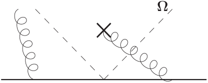
Figure 5.1: A veto of primary emission going into $\Omega$. The kind of LL terms produced by this kind of diagram are understood from resumming independent gluon emission.

To see the origin of these logarithms more clearly, consider soft gluonic radiation into a patch of phase space $\Omega$ arising from a 2 jet system, where we restrict the total energy of radiation into $\Omega$ to be less than $Q_{\Omega}$. The primary logarithms arise from gluons that are emitted directly into $\Omega$, as shown in figure 5.1, with energy vetoed down to a scale $Q_{\Omega}$, which is denoted by a crossed gluon line in the figure, and form the single logarithmic (SL) set $\left(\alpha_{s}\log\frac{Q}{Q_{\Omega}}\right)^{n}$, $n\geq 1$, where $Q$ is the scale of the jet line. Now consider a gluon being emitted outside of $\Omega$ with intermediate energy $Q_{1}$, and then vetoing subsequent emission from this gluon into $\Omega$ down to scale $Q_{\Omega}$, as shown in figure 5.2. Integrating $Q_{1}$ up to $Q$ then generates another SL set of $\left(\alpha_{s}\log\frac{Q}{Q_{\Omega}}\right)^{n}$, $n\geq 2$, which are formally the same order as the primary emission terms. This was studied in detail in [61, 69] and in this work we consider how the conclusions found are modified phenomenologically when the kt clustering algorithm is applied to the final state. This new class of logarithm, which enter at leading log (LL) accuracy in energy flow observables, are known as non-global logarithms (NGLs), as they arise in non-global observables, or as secondary logarithms, as they are produced by secondary gluonic radiation.

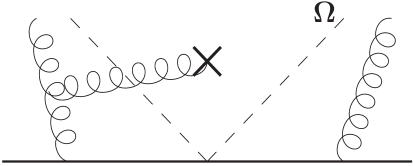
Figure 5.2: A veto of emission into $\Omega$ from a gluon radiated outside of $\Omega$. This configuration will produce a non-global logarithm.

The organisation of this chapter is as follows. We start in section 5.2 with a definition of our observable, and a discussion of how we include NGLs in our calculations. Section 5.3 then describes the kt clustering algorithm used in the H1 and ZEUS analyses, known as the inclusive jet clustering algorithm. We then develop the algorithm, in order to derive a form suitable for use with a 2-jet system. Section 5.4.1 then describes the order $\alpha_{s}^{2}$ calculation of the effect of NGLs in our 2-jet system, with the clustering algorithm included in the calculation. We find that the asymptotic suppression factor with clustering is reduced with respect to the non-clustering case. We then proceed to calculate the non-global effect to all orders in section 5.4.2 using the combination of the large $N_{c}$ limit and a Monte Carlo algorithm and find that the NGLs act as a suppression to the observable, and this suppression is reduced when we impose clustering on the final state. In section 5.5 we give an overview of some of the current research work in the area of non-global observables and finally we conclude with a summary and directions for further work in section 5.6.

To summarise our conclusions, the all-orders treatment used in this chapter allows direct inclusion of the kt algorithm, in exactly the same way as is used experimentally, and we find that the clustering process reduces the magnitude of the non-global corrections to the primary suppression factor. However they are still phenomenologically relevant at HERA. The research work in this chapter is published in [70, 71].

5.2 Non-global logarithms in a 2-jet system

Following Dasgupta and Salam [61], the observable we are interested in is the total transverse energy $E_{t}$ flowing into a region of phase space $\Omega$ for an event characterised by the hard scale $Q$,

$$E_{t}=\sum_{i\in\Omega}E_{t,i}.$$ (5.1)

We are specifically interested in the cases of $\Omega$ being either a slice in rapidity or a patch, bounded in rapidity and azimuthal angle. The quantity we shall calculate is called $\Sigma_{\Omega}$ and is defined to be the probability that $E_{t}$ is less than some energy scale $Q_{\Omega}$,

$$\Sigma_{\Omega}=\frac{1}{\sigma_{o}}\int_{0}^{Q_{\Omega}}dE_{t}\frac{d\sigma}{dE_{t}}.$$ (5.2)

We normalise this equation to the process cross section, for example 2 jet production in $e^{+}e^{-}$ annihilation, and we shall assume the strong ordering $Q_{\Omega}\ll Q$. The aim of this work is to calculate the importance of the non-global contribution to $\Sigma_{\Omega}$ and so it is convenient to factorise this expression into a function describing primary emission into $\Omega$, $\Sigma_{\Omega,P}(t)$, and a function describing (secondary) emission into $\Omega$ from large-angle soft gluons outside of $\Omega$, $S(t)$,

$$\Sigma_{\Omega}(t)=S(t)\Sigma_{\Omega,P}(t).$$ (5.3)

This expression is accurate to LL level (it is helpful to think of this as a probabilistic expression, and the observable can be written as the probability for the region $\Omega$ to stay empty from primary gluons times the probability for the region $\Omega$ to stay empty from secondary gluons) and the primary emission function $\Sigma_{\Omega,P}$ is the 2 jet analogue of what has been calculated for 4 jet systems. We have denoted the following integral of $\alpha_{s}$ by $t$,

$$t(Q_{\Omega},Q) = \frac{1}{2\pi}\int_{Q_{\Omega}}^{Q/2}\frac{dk_{t}}{k_{t}}\alpha_{s}(k_{t}),$$ (5.4)

$$= \frac{1}{4\pi\beta_{0}}\log\left(\frac{\alpha_{s}(Q_{\Omega})}{\alpha_{s}(Q/2)}\right),$$ (5.5)

$$= \frac{\alpha_{s}}{2\pi}\log\frac{Q}{2Q_{\Omega}},$$ (5.6)

where the first equality is exact, the second holds at one loop, the third assumes a fixed coupling and $\beta_{0}=(11C_{A}-2n_{f})/(12\pi)$. The leading order contribution to $S(t)$ comes in at $\alpha_{s}^{2}$ and we shall calculate this for a 2 jet system in the next section but it is useful to first consider the primary emission function at first order in $\alpha_{s}$. If we do not restrict the phase space for gluon emission then, order by order in perturbation theory, we expect a complete cancellation of real and virtual soft gluon contributions to the primary emission form factor. However the requirement of a gap in a restricted region of phase space results in this cancellation being spoilt and we are left with an integral over the vetoed region. Hence, to order $\alpha_{s}$,

$$\Sigma_{\Omega}^{(1)}(Q_{\Omega},Q) = -4C_{F}\frac{\alpha_{s}}{2\pi}\int_{Q_{\Omega}}^{Q/2}\frac{dk_{t}}{k_{t}}\int_{\Omega}d\eta\frac{d\phi}{2\pi},$$ (5.7)

$$= -\frac{4C_{F}\alpha_{s}}{2\pi}A_{\Omega}\log\left(\frac{Q}{2Q_{\Omega}}\right),$$ (5.8)

where $A_{\Omega}$ denotes the area in $(\eta,\phi)$ space of the region $\Omega$. When the energy scales are strongly ordered, the logarithm can become large enough to overcome the smallness of $\alpha_{s}$ and it becomes necessary to include terms like $\left(\alpha_{s}\log\frac{Q}{Q_{\Omega}}\right)^{n}$ to all orders. The assumption that the primary gluons are emitted independently according to a two-particle antenna pattern allows one to exponentiate the one loop answer and run the coupling to the scale $k_{t}$. We can then write $\Sigma_{\Omega,P}(t)$ to all orders,

$$\Sigma_{\Omega,P}(t)=\exp\left(-4C_{F}A_{\Omega}t\right).$$ (5.9)

This equation only includes contributions from independent primary emission. We also need to account for secondary gluon emission, which generates NGLs, through the function $\mathcal{S}(t)$. This has the following expansion in $\alpha_{s}$,

$$\mathcal{S}(t)=1+S_{2}\,t^{2}+S_{3}\,t^{3}+\ldots=1+\sum_{n=2}S_{n}\,t^{n}.$$ (5.10)

Note that $\mathcal{S}(t)$ has its first non-trivial term at order $\alpha_{s}^{2}$ because we need at least two gluons to cause a NGL to appear. The function $\mathcal{S}(t)$ has been studied for a 2 jet system without any final state requirements [61] and the purpose of this work is to calculate the function, at leading and at all orders, with the requirement of kt clustering on the final state. Therefore, before we turn to the details of the calculation of $\mathcal{S}(t)$, let us discuss the kt clustering algorithm.

5.3 The kt clustering algorithm

In this section we shall review the formulation of the kt clustering algorithm which we will use in our calculations. We also provide a formulation that can be directly applied to our fixed order calculation in the next section.

The version of the algorithm we use, which is the one used in the HERA analyses, is known as the inclusive kt algorithm [64, 65, 66]. The main features of importance to the present study are: the clustering procedure starts from the particles of lowest relative transverse momenta and iteratively merges them to construct pseudoparticles of higher transverse momentum; the decision of whether a particular pair of pseudoparticles are merged depends on their relative opening angle and their transverse energy (see below); despite this, it is possible for soft particles to be ‘dragged’ through relatively large angles by being merged with harder particles, which are merged with even harder particles, and so on. Nevertheless, we do not expect our results to be qualitatively different from other infrared safe jet algorithms, such as the improved Legacy Cone algorithm of [72].

In the formulation of the algorithm, we represent the final state of a process by a set of “protojets” $i$ with momenta $p_{i}^{\mu}$. The algorithm works in an iterative way and groups pairs of protojets together to form new ones. The aim is to group almost-parallel protojets together so that they are part of the same protojet. Once certain criteria are met, a protojet is considered a jet and is not considered further. The algorithm therefore needs to specify what it means for two objects to be close together and also how to merge two protojets together. Here we follow the H1 and ZEUS analyses closely and set the radius parameter, $R$, to unity. The procedure is

1. For each protojet, define

   $$d_{i}=E_{T,i}^{2}$$ (5.11)

   and for each protojet pair define

   $$d_{ij}=\mathrm{min}(E_{T,i}^{2},E_{T,j}^{2})[(\eta_{i}-\eta_{j})^{2}+(\phi_{i}-\phi_{j})^{2}]/R^{2}.$$ (5.12)

2. Find the smallest of all the $d_{i}$ and $d_{ij}$, and label it $d_{\mathrm{min}}$.

3. If $d_{\mathrm{min}}$ is a $d_{ij}$, merge protojets $i$ and $j$ into the new protojet $k$ with

   $$E_{T,k}=E_{T,i}+E_{T,j},$$ (5.13)

   and

   $$\eta_{k}=[E_{T,i}\eta_{i}+E_{T,j}\eta_{j}]/E_{T,k},$$

   $$\phi_{k}=[E_{T,i}\phi_{i}+E_{T,j}\phi_{j}]/E_{T,k}.$$ (5.14)

4. If $d_{\mathrm{min}}$ is a $d_{i}$, the corresponding protojet $i$ is not “mergable”. Remove it from the list of protojets and add it to the list of jets. This procedure continues until there are no more protojets. As it proceeds, it produces a list of jets with successively larger values of $d_{i}=E_{T,i}^{2}$.

This algorithm is implemented in the package KTCLUS [73], which is used for the all-orders calculation later in this work.

It is necessary to use the full iterative algorithm for experimental analyses and for Monte Carlo applications, but when we consider a 2 gluon final state in this work we can reduce the algorithm to a convenient analytic form. We start by considering a hard jet line at scale $Q$ which radiates a gluon with some transverse energy $E_{T,1}$ in some direction $(\eta_{1},\phi_{1})$. This gluon then proceeds to radiate a secondary soft gluon with transverse energy $E_{T,2}$ in some direction $(\eta_{2},\phi_{2})$. We assume that the energies of the gluons are strongly ordered,

$$E_{1}\gg E_{2},$$ (5.15)

which implies the same for the transverse energies,

$$E_{T,1}\gg E_{T,2}.$$ (5.16)

Applying the clustering algorithm to the two gluons gives,

$$d_{1} = E_{T,1}^{2},$$

$$d_{2} = E_{T,2}^{2},$$

$$d_{12} = E_{T,2}^{2}[(\eta_{1}-\eta_{2})^{2}+(\phi_{1}-\phi_{2})^{2}]/R^{2}.$$ (5.17)

By considering the strong ordering of the transverse momenta, the two gluons will be clustered if $d_{ij}<d_{2}$, so we require

$$(\eta_{1}-\eta_{2})^{2}+(\phi_{1}-\phi_{2})^{2}>R^{2}$$ (5.18)

for the two gluons to constitute separate jets and not be merged by the algorithm. Therefore for a 2-gluon final state to pollute the gap and generate secondary logarithms we require that gluon 1 is outside the gap, gluon 2 is inside the gap and that they be sufficiently separated in the $(\eta,\phi)$ plane to avoid being merged. The result of this section is that the clustering condition manifests itself as a $\Theta$-function in our calculation,

$$\Theta((\eta_{1}-\eta_{2})^{2}+\phi_{2}^{2}-R^{2}),$$ (5.19)

where we have used our freedom to set $\phi_{1}=0$. We will use this result in the next section. Therefore the clustering procedure, when applied to a 2 gluon system, will pull the softer gluon out of the gap and merge it into the harder gluon, provided they are sufficiently close in the $(\eta,\phi)$ plane; hence we expect that clustering will reduce the impact of NGLs in such systems.

5.4 Controlling the non-global logarithms with kt clustering

In this section we describe our calculation of the NGLs with clustering for a 2-jet system. We contrast our work to the unclustered case and find that the clustering procedure reduces the numerical impact of the NGLs. We then use a Monte Carlo program in the large $N_{c}$ limit to find that this conclusion persists to all orders and we make numerical estimates of the impact of NGL in energy flow measurements at HERA.

5.4.1 The LO result

In this section we will calculate the leading order contribution to the non-global logarithm function $\mathcal{S}(t)$. As has already been shown, this has its first non-trivial term at order $\alpha_{s}^{2}$ and has the perturbative expansion,

$$\mathcal{S}(t)=1+S_{2}\,t^{2}+S_{3}\,t^{3}+\ldots=1+\sum_{n=2}S_{n}t^{n}.$$ (5.20)

Our goal is to calculate the $S_{2}$ piece for $\Omega$ defined as a slice in rapidity of width $\Delta\eta$ with the condition that the topology of the gluon tree satisfies the kt clustering algorithm. We shall initially perform the calculation in terms of the polar angles of the emitted gluons, and then again in terms of the rapidities of the emitted gluons because the latter form of the calculation will turn out to have more convenient properties. A precise definition of $S_{2}$ can be given by following [60, 61] and using the 2 body phase space of the emitted gluons. If we only keep the leading logarithmic piece of the integrals over the momentum fractions, defined by

$$k^{0}_{i}=x_{i}\frac{Q}{2},$$ (5.21)

we obtain the following expression for $S_{2}$,

$$S_{2}\log^{2}\left(\frac{Q}{2Q_{\Omega}}\right)+\mathcal{O}\left(\log\left(\frac{Q}{2Q_{\Omega}}\right)\right)=-C_{F}C_{A}\int_{k_{1}\not\in\Omega}d\cos\theta_{1}\frac{d\phi_{1}}{2\pi}$$

$$\int_{k_{2}\in\Omega}d\cos\theta_{2}\frac{d\phi_{2}}{2\pi}\frac{Q^{4}}{16}\int_{0}^{1}x_{2}dx_{2}\int_{x_{2}}^{1}x_{1}dx_{1}\Theta\left(x_{2}-\frac{2Q_{\Omega}}{Q}\right)W_{S}.$$ (5.22)

Therefore $S_{2}$ is the coefficient of the logarithm-squared term in the expansion of $\mathcal{S}(t)$. The limits on the angular integration ensure that gluon 2 enters region $\Omega$ while gluon 1 does not. This expression for $S_{2}$ contains the secondary part, $W_{S}$, of the well-known squared-matrix element for the energy ordered emission of two gluons, which can be derived from standard techniques [74],

$$W = 4C_{F}\frac{(ab)}{(a1)(1b)}\left(\frac{C_{A}}{2}\frac{(a1)}{(a2)(21)}+\frac{C_{A}}{2}\frac{(b1)}{(b2)(21)}+\left(C_{F}-\frac{C_{A}}{2}\right)\frac{(ab)}{(a2)(2b)}\right),$$ (5.23)

$$= C_{F}^{2}W_{P}+C_{F}C_{A}W_{S},$$

where the notation $(ij)$ denotes the dot product of the appropriate 4-momenta. This expression contains the primary emission piece $W_{P}$, proportional to $C_{F}^{2}$, and the piece that interests us, which is the part proportional to $C_{F}C_{A}$ and denoted $W_{S}$. Note that the last term is the dipole interference term and is absent in the large $N_{c}$ limit. We shall begin by writing the 4-momenta in terms of the polar angles of the emitted gluons,

$$k_{a} = \frac{Q}{2}(1,0,0,-1),$$ (5.24)

$$k_{b} = \frac{Q}{2}(1,0,0,1),$$ (5.25)

$$k_{1} = x_{1}\frac{Q}{2}(1,0,\sin\theta_{1},\cos\theta_{1}),$$ (5.26)

$$k_{2} = x_{2}\frac{Q}{2}(1,\sin\theta_{2}\sin\phi_{2},\sin\theta_{2}\cos\phi_{2},\cos\theta_{2}),$$ (5.27)

where the indices $a$ and $b$ refer to quarks, the indices $1$ and $2$ refer to radiated gluons and we have set $\phi_{1}=0$. If we evaluate the 4-momenta products we get

$$(ab) = \frac{Q^{2}}{2},$$ (5.28)

$$(1a) = \frac{Q^{2}x_{1}}{4}(1-\cos\theta_{1}),$$ (5.29)

$$(1b) = \frac{Q^{2}x_{1}}{4}(1+\cos\theta_{1}),$$ (5.30)

$$(2a) = \frac{Q^{2}x_{2}}{4}(1-\cos\theta_{2}),$$ (5.31)

$$(2b) = \frac{Q^{2}x_{2}}{4}(1+\cos\theta_{2}),$$ (5.32)

$$(12) = \frac{Q^{2}x_{1}x_{2}}{4}(1-\sin\theta_{1}\sin\theta_{2}\cos\phi_{2}-\cos\theta_{1}\cos\theta_{2}).$$ (5.33)

Inserting these results into equation (5.23) we obtain

$$W_{S} = \frac{32}{Q^{4}}\frac{1}{(x_{1}x_{2})^{2}}\Bigg{(}\frac{1}{(1+\cos\theta_{1})(1-\cos\theta_{2})(1-\sin\theta_{1}\sin\theta_{2}\cos\phi_{2}-\cos\theta_{1}\cos\theta_{2})}$$ (5.34)

$$+\frac{1}{(1-\cos\theta_{1})(1+\cos\theta_{2})(1-\sin\theta_{1}\sin\theta_{2}\cos\phi_{2}-\cos\theta_{1}\cos\theta_{2})}$$

$$-\frac{2}{(1+\cos\theta_{1})(1-\cos\theta_{1})(1+\cos\theta_{2})(1-\cos\theta_{2})}\Bigg{)}.$$

We shall write the angular part of $W_{s}$ (the part without the overall constant) as $\hat{W}_{s}$. Inserting this result into equation (5.22) and then performing the straightforward energy fraction integrals (the $\Theta$-function ensures that sufficient energy reaches the gap region $\Omega$), where we have kept the leading logarithmic piece (dominant when $Q_{\Omega}/Q$ is small),

$$\int_{0}^{1}\frac{dx_{2}}{x_{2}}\int_{x_{2}}^{1}\frac{dx_{1}}{x_{1}}\Theta\left(x_{2}-\frac{2Q_{\Omega}}{Q}\right)=\frac{1}{2}\log^{2}\left(\frac{2Q_{\Omega}}{Q}\right),$$ (5.35)

we arrive at an expression for $S_{2}$

$$S_{2}=-C_{F}C_{A}\int_{angles}\hat{W}_{S}.$$ (5.36)

Specialising to a slice in rapidity of width $\Delta\eta$, delimited by $\cos\theta=\pm c$ and centred on $\eta=0$ we can exploit the symmetry of the $c_{1}$ integral and perform the $\phi_{1}$ integral to express the integral over angles as

$$\int_{angles}=2\int_{-1}^{-c}d\cos_{1}\int_{-c}^{+c}d\cos_{2}\int_{0}^{2\pi}\frac{d\phi_{2}}{2\pi}.$$ (5.37)

The polar angle integration region is shown in figure 5.3.

Figure 5.3: The integration region for the polar angle integrations of the emitted gluons. Gluon 1 is emitted outside of the gap, and subsequently emits gluon 2 into the gap.

For the case of no clustering of the gluons it is possible to perform the azimuthal average using the result,

$$\int_{0}^{2\pi}\frac{d\phi_{2}}{2\pi}\frac{1}{1-\sin\theta_{1}\sin\theta_{2}\cos\phi_{2}-\cos\theta_{1}\cos\theta_{2}} = \frac{1}{|\cos\theta_{2}-\cos\theta_{1}|},$$ (5.38)

$$= \frac{1}{\cos\theta_{2}-\cos\theta_{1}},$$

where we have exploited the angular ordering of the gluons in writing the second equality. This results in the following, azimuthal-averaged, expression for the matrix element,

$$\langle W_{S}\rangle_{\phi}=4\left(\frac{1}{(1+\cos\theta_{2})(1-\cos\theta_{1})(\cos\theta_{2}-\cos\theta_{1})}\right),$$ (5.39)

with two remaining $\cos\theta$ integrations. For this case of no clustering of the gluons, these remaining integrations have been performed, resulting in the following expression for $S_{2}$ [61],

$$S_{2}=-4C_{F}C_{A}\left[\frac{\pi^{2}}{12}+(\Delta\eta)^{2}-\Delta\eta\log(e^{2\Delta\eta}-1)-\frac{1}{2}\mathrm{Li}_{2}(e^{-2\Delta\eta})-\frac{1}{2}\mathrm{Li}_{2}(1-e^{2\Delta\eta})\right],$$ (5.40)

which, following the literature, we have expressed in terms of $\Delta\eta$, which is related to $c$ by the kinematical relation,

$$\Delta\eta=\ln\left(\frac{1+c}{1-c}\right).$$ (5.41)

We have used the dilogarithm function, which is defined

$$\mathrm{Li}_{2}(y)=\int_{y}^{0}\frac{\log(1-x)}{x}\,dx.$$ (5.42)

We can now use the following identities (with $x=~{}\exp(-2\Delta\eta)$ in the first identity and $x=\exp(2\Delta\eta)$ in the second identity),

$$\mathrm{Li}_{2}(x) = \frac{\pi^{2}}{6}-\log(x)\log(1-x)-\mathrm{Li}_{2}(1-x),$$ (5.43)

$$\mathrm{Li}_{2}(1-x) + \mathrm{Li}_{2}(1-x^{-1})=-\frac{1}{2}\log^{2}(x),$$ (5.44)

to write this result as

$$S_{2}=-4C_{F}C_{A}\left[\frac{\pi^{2}}{6}-\mathrm{Li}_{2}(e^{-2\Delta\eta})\right].$$ (5.45)

Note that as $\Delta\eta$ increases, $S_{2}$ rapidly saturates at its asymptotic value,

$$\lim_{\Delta\eta\rightarrow\infty}=-C_{F}C_{A}\frac{2\pi^{2}}{3},$$ (5.46)

since we note that $\mathrm{Li}_{2}(0)=0$. This analytic evaluation of $S_{2}$ is not possible for the case of clustered gluons because, as discussed previously, the requirement that a gluonic final state is in a configuration that will survive the clustering algorithm can be written as a $\Theta$-function of all three angular integration variables,

$$\Theta((\eta_{1}-\eta_{2})^{2}+\phi_{2}^{2}-R^{2}).$$ (5.47)

In this situation we have to resort to a numerical solution, in which we integrate over the three remaining variables. This method has the advantage of being easily extendible to any gap geometry of interest. It is possible, however, to obtain a result for $S_{2}$ with clustering which is expressible as a 1D integral by using the rapidity of the emitted gluons. This has the advantage of requiring a simpler method of numerical solution. In analogy with equation (5.22), we can express $S_{2}$ in terms of the gluon rapidities,

$$-C_{F}C_{A} \int_{k_{1}\not\in\Omega}d\eta_{1}\frac{d\phi_{1}}{2\pi}\int_{k_{2}\in\Omega}d\eta_{2}\frac{d\phi_{2}}{2\pi}\frac{Q^{4}}{16}\int_{0}^{1}x_{2}dx_{2}\int_{x_{2}}^{1}x_{1}dx_{1}\Theta\left(x_{2}-\frac{2Q_{\Omega}}{Q}\right)W_{S}$$ (5.48)

$$=S_{2}\log^{2}\left(\frac{Q}{2Q_{\Omega}}\right)+\mathcal{O}\left(\log\left(\frac{Q}{2Q_{\Omega}}\right)\right).$$

Note that in this equation, $x_{1}$ and $x_{2}$ are defined as transverse momentum fractions,

$$P_{t,1}=x_{1}\frac{Q}{2},$$ (5.49)

and not energy fractions as they are in equation (5.22), which was written in terms of polar angles. However, this does not affect the result. The definition of $Q_{\Omega}$ has also correspondingly changed. We can relate the phase space in the two coordinate systems by

$$\frac{d^{3}\vec{k}}{k^{0}}=k_{t}\,dk_{t}\,d\eta\,d\phi.$$ (5.50)

We begin by defining the following 4-momenta,

$$k_{a} = \frac{Q}{2}(1,0,0,-1),$$ (5.51)

$$k_{b} = \frac{Q}{2}(1,0,0,1),$$ (5.52)

$$k_{1} = P_{t,1}(\cosh\eta_{1},\sin\phi_{1},\cos\phi_{1},\sinh\eta_{1}),$$ (5.53)

$$k_{2} = P_{t,2}(\cosh\eta_{2},\sin\phi_{2},\cos\phi_{2},\sinh\eta_{2}),$$ (5.54)

where the indices are the same as those defined for the polar angle calculation. Evaluating the 4-momenta products we get

$$(ab) = \frac{Q^{2}}{2},$$ (5.55)

$$(1a) = \frac{Q^{2}x_{1}}{4}\exp(-\eta_{1}),$$ (5.56)

$$(1b) = \frac{Q^{2}x_{1}}{4}\exp(+\eta_{1}),$$ (5.57)

$$(2a) = \frac{Q^{2}x_{2}}{4}\exp(-\eta_{2}),$$ (5.58)

$$(2b) = \frac{Q^{2}x_{2}}{4}\exp(+\eta_{2}),$$ (5.59)

$$(12) = \frac{Q^{2}x_{1}x_{2}}{4}\left(\cosh(\eta_{1}-\eta_{2})-\cos(\phi_{1}-\phi_{2})\right).$$ (5.60)

Inserting these results into the expression for $W_{S}$, equation (5.23) and using our freedom to set the azimuthal angle of the first gluon to zero, $\phi_{1}=0$, we obtain

$$W_{S}=\frac{128}{Q^{4}x_{1}^{2}x_{2}^{2}}\left(\frac{\cosh(\eta_{1}-\eta_{2})}{\cosh(\eta_{1}-\eta_{2})-\cos\phi_{2}}-1\right).$$ (5.61)

The transverse momentum fraction integrals are straightforward, as before,

$$\int_{0}^{1}\frac{dx_{2}}{x_{2}}\int_{x_{2}}^{1}\frac{dx_{1}}{x_{1}}\Theta\left(x_{2}-\frac{2Q_{\Omega}}{Q}\right)=\frac{1}{2}\log^{2}\left(\frac{2Q_{\Omega}}{Q}\right).$$ (5.62)

Specialising to a slice in rapidity of width $\Delta\eta$ and delimited by $|\eta|<\Delta\eta/2$, where boost invariance allows us to centre the gap on $\eta=0$, we can exploit the symmetry of the $\eta_{1}$ integral and perform the trivial $\phi_{1}$ integral of the first gluon to express the final integral over angles as

$$\int_{angles}=2\int_{-\infty}^{-\frac{\Delta\eta}{2}}d\eta_{1}\int_{-\frac{\Delta\eta}{2}}^{\frac{\Delta\eta}{2}}d\eta_{2}\int_{0}^{2\pi}\frac{d\phi_{2}}{2\pi}.$$ (5.63)

The rapidity integration region is shown in figure 5.4.

Figure 5.4: The integration region for the rapidity integrations of the emitted gluons. Gluon 1 is emitted outside of the gap, and subsequently emits gluon 2 into the gap.

For the case of no clustering of the gluons it is possible to perform the azimuthal average using the result,

$$\int_{0}^{2\pi}\frac{d\phi_{2}}{2\pi}\frac{1}{\cosh(\eta_{1}-\eta_{2})-\cos\phi_{2}}=\frac{1}{|\sinh(\eta_{1}-\eta_{2})|}.$$ (5.64)

This can be elegantly proven by noting that the following contour integration over the unit circle,

$$I=\frac{i}{\pi}\oint_{u_{1}}\frac{dz}{(z-\exp(\eta_{2}-\eta_{1}))(z-\exp(\eta_{1}-\eta_{2}))},$$ (5.65)

is equivalent to the integration over the azimuthal angle of the second gluon. To see this, expand the $\cosh(\eta_{1}-\eta_{2})$ and $\cos(\phi_{2})$ as exponentials and write $z=\exp(i\phi_{2})$. We get poles at

$$z=e^{y},\,e^{-y},$$ (5.66)

where $y=\eta_{1}-\eta_{2}$. We only have to consider the poles which satisfy $|z|<1$, which is $z=\exp(-|y|)$, so

$$I = 2\pi i\left(\frac{i}{\pi}\right)\lim_{z\rightarrow\exp(-|y|)}\left\{\frac{z-\exp(-|y|)}{(z-\exp(-|y|))(z-\exp(|y|))}\right\},$$ (5.67)

$$= -\frac{2}{\exp(-|y|)-\exp(|y|)},$$

$$= \frac{1}{\sinh(|y|)},$$

and write $\sinh(|y|)=|\sinh(y)|$. As for the polar angle case, it is possible to do all the integrations for the case of no clustering. However, evaluation of $S_{2}$ is not possible for the case of clustered gluons because, as discussed previously, the requirement that a gluonic final state is in a configuration that will survive a clustering algorithm appears as a $\Theta$-function in our calculation, and the argument of the $\Theta$-function is very complicated. However we can readily reduce the three-dimensional integral to a one-dimensional integral using standard techniques if we consider the region of phase space that is vetoed by the clustering algorithm, denoted $S_{2}^{v}$. Doing this we obtain,

$$S_{2}^{v} = \frac{-32C_{F}C_{A}}{\pi}\int_{0}^{R}\mathrm{min}(\eta,\Delta\eta)\bigg{[}2\coth(\eta)\times$$

$$\arctan\left(\frac{\tan(\sqrt{R^{2}-\eta^{2}}/2)}{\tanh(\eta/2)}\right)-\sqrt{R^{2}-\eta^{2}}\bigg{]}d\eta,$$

where we define $\eta=\eta_{1}-\eta_{2}$. This result is proved in appendix C. Therefore the solution for $S_{2}$ with the clustering condition imposed is obtained by subtracting $S_{2}^{v}$ from the analytic unclustered result. We resort to numerical techniques to solve this equation, which has the advantage of being easily extendible to any gap geometry of interest. Our numerics were done using Monte Carlo integration methods and the routine Vegas. Figure 5.5 shows our result for $S_{2}$ as a function of the gap width $\Delta\eta$ and with the radius parameter, $R$, set to 1. The solid line is $S_{2}$ without clustering and the dotted line is $S_{2}$ with clustering.

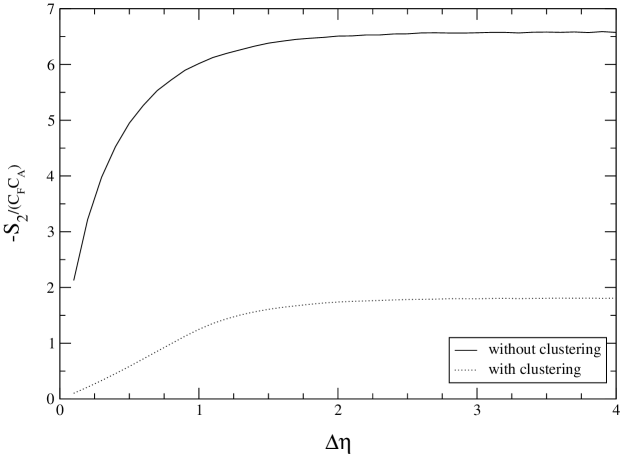
Figure 5.5: $S_{2}$ as a function of $\Delta\eta$. The clustered curve is obtained using a kt algorithm with a radius parameter of 1.0.

In [61], where the unclustered case was first obtained, the observed saturation was given a simple physical explanation: the dominant contribution to $S_{2}$ comes from regions where the two gluons are close together (which means that gluon 1 is just outside the gap and gluon 2 is just inside the gap.) This occurs when

$$\eta_{1}\simeq\eta_{2}\simeq-\Delta\eta/2,$$ (5.69)

and the dominant contribution arises from the collinear region of the matrix element. Therefore at large $\Delta\eta$, $S_{2}$ received no contribution from the centre of the gap, only the edges, and the value of $-S_{2}/(C_{F}C_{A})$ saturates. This is the reason that NGLs are often referred to as an ‘edge effect’, and gluons closest to the boundary of the restricted region of phase space make the largest contribution. This effect is illustrated in figure 5.6.

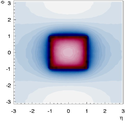
Figure 5.6: Contributions to the leading order NGLs for a patch in rapidity, as a function of rapidity and azimuthal angle. Darker shades correspond to a larger contribution and it can be seen that the largest contribution comes from the edge of the patch. This figure is taken from [71].

We note that $S_{2}^{v}$ itself saturates when $\Delta\eta\simeq R$. The results we have obtained show that when we demand the gluonic final state to survive a clustering algorithm, the saturation of $S_{2}$ observed in [61] is still observed but the saturation value is reduced by $70\%$. In other words the value that $-S_{2}/(C_{F}C_{A})$ saturates to is reduced from $6.57$ to $1.81$. The reason for this reduction is that we have removed gluons from the region of collinear enhancement, but gluons that are still sufficiently separated in the $(\eta,\phi)$ plane to satisfy

$$(\eta_{1}-\eta_{2})^{2}+\phi_{2}^{2}>R^{2},$$ (5.70)

will survive the clustering process and contribute to the NGLs. Therefore we conclude that the saturation of the non-global contribution at fixed order is still seen when we demand clustering of the final state.

5.4.2 Non-global logarithms to all orders

The analytic treatment of the 2 gluon system, with or without clustering, is fairly straightforward. The extension to the many-gluon case presents considerable problems due to the geometry and the colour structure of the ‘mexican cactus’ gluon ensemble. Therefore we have extended our calculation to all orders by working in the large $N_{c}$ limit and by employing numerical methods. The complicated colour algebra one obtains is simplified in the large $N_{c}$ limit, because the squared-matrix element for the gluon radiation can be broken down into a series of independent terms, each associated with a different colour dipole. The complicated geometry of multi-gluon events is handled by use of a Monte Carlo algorithm, in which the gluon cascade is built up from successive dipole branching. Therefore we start with a single colour dipole, representing the initial quark line, which emits a gluon and splits into two dipoles, which themselves may go on to emit. The cascade carries on until an emitted gluon enters the gap region. This method also allows the kt clustering algorithm to be directly implemented, in exactly the same way it is used experimentally, and before a given gluon configuration can be deemed to have polluted the gap it must survive the algorithm. If the gluon which has entered the gap is pulled out by the clustering procedure, then the dipole cascade is allowed to continue.

Note that there are a lot of configurations with many gluons at high $t$ and this, coupled with the fact that the speed of the kt algorithm scales like $N^{3}$ (where $N$ is the number of gluons), means that the Monte Carlo algorithm can be very slow in this region. The result is that we have large statistical errors for $t\geq 0.3$, so we do not show this region.

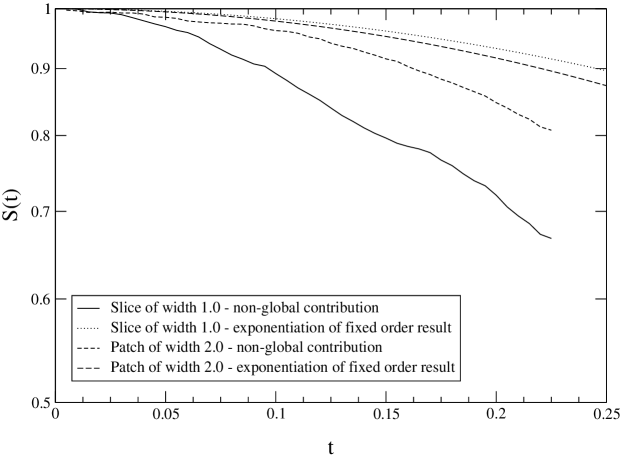
Figure 5.7: The function $S(t)$ for a slice and a patch of phase space, with the condition of kt clustering imposed on the gluons. These curves were obtained using a Monte Carlo procedure in the large $N_{c}$ limit. Also shown are the curves for $S(t)$ obtained by exponentiating the fixed order result. The geometry independence of the $t$ dependence indicates that the buffer zone mechanism identified to exist in previous work survives the clustering algorithm. Note that the slice shows greater non-global suppression than the patch at high $t$, in contrast to the unclustered case [61].

We have verified the results obtained by Dasgupta and Salam [61], which have been calculated with no clustering requirement imposed on the gluons, and written a program, based on their program, to perform the all-orders calculation with clustering.

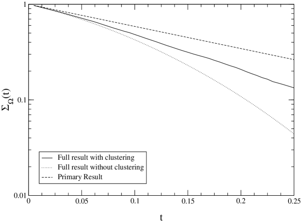
Figure 5.8: The phenomenological implications of clustering for the case of $\Omega$ being a slice of rapidity of width $1.0$. The reduction of the non-global suppression factor when clustering is included can be seen.

Figure 5.7 shows the function $S(t)$ for two different geometries for $\Omega$: a slice in rapidity of width $\Delta\eta=1.0$ and a square patch in rapidity and azimuthal angle of side length $\Delta\eta=\Delta\phi=2.0$, with the requirement of clustering on the final state gluons. The curves labelled ‘exponentiation of the fixed order result’ are those obtained if there were a simple exponentiation of the $S_{2}$ term.

Firstly the figure shows that at high $t$ ($t>0.2$) the suppression increases faster for the full calculation than for the exponentiation of $S_{2}$ with clustering and the two curves have different shapes in this region. This implies a more complex geometry dependence in the full result than is seen by the simple exponentiation of $S_{2}$. Secondly we see that the $t$ dependence of the suppression is geometry (i.e. the definition of $\Omega$) independent at high $t$; the implication of this is that the clustering process maintains a so-called buffer region of suppressed intermediate radiation around $\Omega$. Such a buffer mechanism has been postulated to exist in the unclustered case, and be responsible for the lack of gluons in the gap region. Therefore figure 5.7 shows that the all-orders result with clustering is more complicated than simple exponentiation of the fixed order result. Our work also indicates, due to the geometry independence at high $t$, that a buffer region exists around the gap $\Omega$ which is responsible for the suppression of radiation into the gap.

Figure 5.8 shows the reduction of the phenomenological significance of the NGLs when we cluster the final state. The figure shows the function $\Sigma(t)$ with only primary emissions and the full all-orders treatment with and without clustering effects. This is done with $\Omega$ defined as a slice in rapidity of size $\Delta\eta=1.0$. There are several points to note. Firstly the effect of the NGLs is a large suppression of the cross section relative to the primary-only result. The value of $t$ which we can consider the realistic upper limit for Tevatron Run II experiments is about $0.15$ so we shall take $t=0.15$ as our reference value. We can translate this into an energy scale by using the running coupling definition of $t$, equation (5.5), and obtain $Q\sim 100$ GeV for $Q_{\Omega}=1$ GeV. In this region the inclusion of the non-global effects without clustering increases the suppression relative to the primary-only result by about a factor of $1.65$. When we include clustering effects, this difference is reduced to about $1.2$. Therefore, at all orders, the requirement of clustering on the final state reduces the phenomenological significance of the non-global effects by about 70%. This reduction in magnitude of the effect can be seen to persist to all orders. Hence when calculating cross sections, if we exclude the effect of NGLs then we will overestimate the cross section by $65\%$ for a non-clustered final state and by $20\%$ for a clustered final state. At larger $t$ values, the overestimation increases. For comparison, the typical errors on the H1 gaps-between-jets data is $\sim 30\%$.

Finally, figure 5.9 shows the same comparison of the full result, with and without clustering, for a patch of size $\Delta\eta=\Delta\phi=2.0$. We can see that the conclusions we made for figure 5.8 apply and the effect of the NGLs is of similar magnitude.

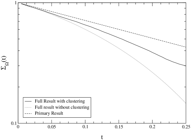
Figure 5.9: The effect of the clustering of the gluons on the function $S(t)$ for a patch of phase space of size $\Delta\eta=\Delta\phi=2.0$.

We have also performed calculations to see how the non-global suppression is affected by varying the radius parameter, $R$, of the clustering procedure. Figure 5.10 shows the full function $\Sigma_{\Omega}$ with NGLs included and with varying $R$. By decreasing $R$ the impact of the clustering algorithm is reduced and the effect of the NGLs is restored to the non-clustered case. In fact, we expect the magnitude of the non-global suppression to tend to the non-clustered case as $R\rightarrow 0$. Similarly, increasing the radius causes more gluons to be included in the clustering and hence the magnitude of the suppression to reduce. In fact, we have found that for $R$ close to $1.5$ the full result is almost identical to the primary result.

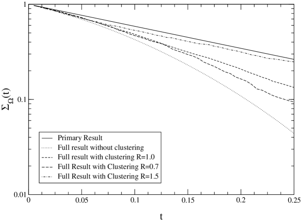
Figure 5.10: The effect of varying radius parameter on the full function $\Sigma_{\Omega}$, for a slice in rapidity of width $\Delta\eta=1.0$.

In summary, non-global logarithms are important not only from the point of view of correctness of the leading logarithm series but also result in significant numerical corrections to cross sections. These corrections are reduced by about a factor of 3 if we cluster the final state. It is clear, therefore, that while the use of the kt algorithm has aided the control of the NGLs, they still have a significant numerical effect at HERA.

5.5 Ongoing research topics in non-global observables

Non-global observables are a new and exciting research area in QCD. In this review section, we will give an brief overview of some current research directions and the progress made.

5.5.1 The 4 jet system

In this section, we will introduce the calculation of NGLs for a 4 jet system, working in the large $N_{c}$ limit at fixed order. This is physically motivated by the wish to understand the effect of NGLs for hadrons to jets in, for example, rapidity gap event in photoproduction. The main difference between a 2 jet system and a 4 jet system is the greater number of dipole radiation sources in the latter case. We model the 4 jet system in the large $N_{c}$ limit, using non-interacting and recoilless dipoles. The initial state jets have 4-momenta,

$$a^{\mu} = \frac{Q}{2}(1,0,0,1),$$

$$b^{\mu} = \frac{Q}{2}(1,0,0,-1),$$ (5.71)

and the final state jets have 4-momenta,

$$c^{\mu} = p_{t}^{c}(\cosh(\Delta\eta/2),1,0,\sinh(\Delta\eta/2)),$$

$$d^{\mu} = p_{t}^{d}(\cosh(\Delta\eta/2),-1,0,-\sinh(\Delta\eta/2)).$$ (5.72)

In this work we assume that the jets are produced at fixed $\Delta\eta=|\eta_{1}-\eta_{2}|$. The matrix element squared for emitting a gluon can be written, in the large $N_{c}$ limit as

$$W_{1}=4C_{F}\left(\frac{(ad)}{(a1)(1d)}+\frac{(bc)}{(b1)(1c)}\right),$$ (5.73)

where the first term describes the probability of the gluon being emitted from the $(ad)$ dipole, and the second term describes the probability of the gluon being emitted from the $(bc)$ dipole. There is, of course, other terms describing $s$ and $t$ channel dipole emission but we initially restrict ourselves to equation (5.73) for simplicity. In these equations the notation $(ij)$ means the scalar product of the corresponding 4-momenta and we write the 4-momentum of the emitted gluon by

$$\mathbbm{1}^{\mu}=p_{t}^{1}(\cosh\eta_{1},\cos\phi_{1},\sin\phi_{1},\sinh\eta_{1}).$$ (5.74)

The matrix element squared for the first gluon to emit a second gluon is, in the same approximation

$$W_{S} = 4C_{F}\frac{(ad)}{(a1)(1d)}\left(\frac{C_{A}}{2}\frac{(a1)}{(a2)(21)}+\frac{C_{A}}{2}\frac{(1d)}{(d2)(21)}\right)$$ (5.75)

$$+ 4C_{F}\frac{(bc)}{(b1)(1c)}\left(\frac{C_{A}}{2}\frac{(b1)}{(b2)(21)}+\frac{C_{A}}{2}\frac{(1c)}{(c2)(21)}\right),$$

where

$$\mathbbm{2}^{\mu}=p_{t}^{2}(\cosh\eta_{2},\cos\phi_{2},\sin\phi_{2},\sinh\eta_{2}).$$ (5.76)

By proceding in analogy to the fixed order calculation for a 2 jet system, we may extract the non-global suppression factor for a hadron-hadron process which produces 2 jets at fixed $\Delta\eta$. The physical expectation is that the greater quantity of dipole sources will give a larger non-global suppression factor for a 4 jet system, relative to the 2 jet case. The 2-jet all orders calculation can be extended in a similar way, to extract the all-orders 4-jet non-global suppression factor, as a function of the gap width and the time-energy variable $t$. Such a study is being performed at present.

5.5.2 Event shape/energy flow correlations

Another way of reducing the phenomenological impact of NGLs, in addition to the use of clustering algorithms, has been proposed [75], and is the study of associated distributions in two variables. In this work, one combines measurement of a jet shape $V$ in the whole of phase space (for example thrust, $V=1-T$) and that of the transverse away-from-jets energy flow $E_{\mathrm{out}}$. The former is a global measurement and the latter is a non-global measurement. If the observable $V$ selects 2-jet-like configurations, one measures the associated distribution,

$$\Sigma_{\mathrm{2ng}}(Q,V,E_{out}),$$ (5.77)

where $Q$ is the hard scale. It has been shown that this distribution factorises [76],

$$\Sigma_{\mathrm{2ng}}(Q,V,E_{out})=\Sigma(Q,V)\cdot\Sigma_{\mathrm{out}}(VQ,E_{\mathrm{out}}),$$ (5.78)

where $\Sigma(Q,V)$ is the standard global distribution of $V$ and $\Sigma_{\mathrm{out}}(VQ,E_{\mathrm{out}})$ contains the logarithmic distribution in $E_{\mathrm{out}}$. This latter distribution, containing NGLs is evaluated at the reduced scale $VQ$, and hence the logarithmic terms will be $(\alpha_{s}\log(VQ/E_{\mathrm{out}}))^{n}$. The work of Berger, Kúcs and Sterman[75] considered the region in which $VQ$ and $E_{\mathrm{out}}$ were comparable, so that the NGLs give a negligible contribution. Thus, for a restricted subset of appropriately selected events, it is possible, to ‘tune out’ the non-global logarithmically enhanced terms in associated distributions. Hence the use of event shape/energy flow correlations is another method, along with clustering algorithms, to control the effect of NGLs in non-global observables.

5.6 Conclusions

The observation that observables that are sensitive to radiation in only a restricted part of phase space, so-called non-global observables, are strongly sensitive to secondary radiation is a new and exciting discovery. For a long time it was widely thought, now it seems incorrectly, that it was sufficient to consider only primary emission contributions to such observables. These primary, or Bremsstrahlung, contributions are well understood for a variety of processes. Recent measurements of gaps-between jets events at H1 and ZEUS are exactly the class of observable that are sensitive to these effects and to deal with this fact, a study of NGLs in the context of HERA measurements is required. In this chapter we considered the NGLs generated from secondary radiation into a restricted region of phase space under the condition of the final state surviving a clustering algorithm. Such kt clustering algorithms have been used for the HERA measurements. Our work verified the study of Dasgupta and Salam, who found that inclusion of NGLs resulted in a strong suppression of the theoretical prediction of the non-global observable.

We have also studied the NGLs for a 2 jet system with clustering imposed and found that the clustering process reduced, but did not eliminate, the non-global logarithm effect.

Our main conclusion is that the final state specified in the H1 and ZEUS analysis will mean that a primary emission calculation in the manner of Sterman et al [59, 58, 55], and chapter 4, of energy flow observables will overestimate the observed gaps-between-jets rate by around 20%. This is to be contrasted with an overestimation of 65% that would be found for a non-clustered final state. This result was calculated to all orders in the large $N_{c}$ limit for a 2 jet system. The extension of both these results to beyond the large $N_{c}$ limit would be a major step forward in the understanding of these effects in non-global observables and we reserve this for future work.

Chapter 6 Resummation of energy flow observables

6.1 Introduction

The subject of interjet energy flow [77] has attracted considerable interest ever since it was proposed [78, 79] as a way to study rapidity gap processes using the tools of perturbation theory. Rapidity gap processes are defined as processes containing two high $p_{t}$ jets with the region of rapidity between the jets containing nothing more than soft radiation. This region is known generically as the gap. The presence of a range of scales offers a chance to study the interface between the soft, non-perturbative scales and the hard, perturbative scales of QCD.

In this chapter we will calculate the perturbative contribution to gaps-between-jets cross sections in photoproduction at HERA, which have been measured by the H1 [62] and ZEUS [80, 63] collaborations. A feature of the recent analyses is the use of a clustering algorithm to define the hadronic final state and hence the gap. The restriction of transverse radiation in a region of phase space, defined as $\Omega$ and directed away from the observed jets and the beam directions, produces logarithms at each order of QCD perturbation theory of the interjet energy flow, $Q_{\Omega}$, over some hard scale, $Q$. The precise definition of the restricted region, or gap, is totally free and in this work we are interested in the gap region defined by experimental rapidity gap analyses. The source of the large logarithms is twofold. The so-called primary (or global) logarithms arise from radiation emitted directly into $\Omega$; these wide-angle gluons decouple from the dynamics of the colour-diagonal jets and are described by an effective, eikonal theory [55, 59, 58, 53, 7]. The second source of leading logarithms arise from gluons emitted outside of the gap region, an area of phase space generically denoted as $\bar{\Omega}$, which subsequently radiate into $\Omega$. These terms are known as non-global (secondary) logarithms, or NGLs [60, 61, 70, 71], and were introduced in chapter 5.

The primary logarithms are resummed using the formalism of Collins, Soper and Sterman (CSS) [6, 52, 48, 7], which was introduced in chapter 4. In this method the cross section is factorised into a soft part describing the emission of soft, wide angle gluons up to scale $Q_{\Omega}$ and a hard part, describing harder quanta. A unique feature of QCD is that the soft and the hard functions are expressed as matrices in the space of possible colour flow of the system. The scale invariance and factorisation properties of the cross section are then exploited to resum primary logarithms of $Q_{\Omega}/Q$. This resummation is driven by the ultraviolet pole parts of eikonal Feynman graphs and we write the resummed cross section in terms of the eigenvalues of $\Omega$-dependent soft anomalous dimension matrices. These matrices are known for gap definitions based on the cone definition of the final state [59, 58] and for a gap defined as a square patch in rapidity and azimuthal angle [55]; here we are interested in gaps defined in terms of the clustering algorithms employed in the recent analyses. Hence we are required to calculate the corresponding anomalous dimension matrices.

The NGLs [61, 60] are unable to be incorporated into the resummation of the primary logarithms, because the gluon emission patterns that produce the NGLs are sensitive to underlying colour flows not included in the formalism. The effect of NGLs, which is a suppressive effect, on energy flow processes has been studied using numerical methods in the large $N_{c}$ limit and overall factors describing their effect have been extracted for a two jet system, both without [61] and with [70] clustering. The latter case was described in chapter 5. This factor is not directly applicable to the 4 jet systems relevant in the photoproduction of jets but, in the lack of a four jet formalism, we nevertheless use the 2-jet factor in our predictions.

Our aim is to derive LL resummed predictions for the gap cross section, with primary logarithms correct to all orders and secondary logarithms correct in the large $N_{c}$ limit. The gap cross section will follow the HERA analyses and demand two hard jets, defined using the kt clustering algorithm [64, 65, 66], and we will closely follow the H1 and ZEUS gap definition. The technical aspects of soft gluon resummation give a strong dependence on the gluon emission phase space, and hence a considerable part of our work will be concerned with the calculation of soft gluon effects for the specific detector geometry of the H1 and ZEUS experiments.

The organisation of this chapter is as follows. Section 6.2 describes, in detail, the energy flow analyses of H1 and ZEUS. We summarise the experimental cuts employed and the range of measured observables. We also discuss the theoretical implementation of the inclusive kt algorithm employed to define the hadronic final state and the impact on soft gluon resummation. Section 6.3 describes the theoretical definition of our cross section and we employ the standard QCD factorisation theorems to write it as the convolution of non-perturbative parton distributions and a short-distance hard scattering function. We then proceed to refactorise the hard scattering function and exploit this factorisation to resum the large interjet logarithms. Section 6.4 then derives the soft anomalous dimension matrices for the kt defined final state and in section 6.5 we present detailed predictions of rapidity gap processes and compare to the H1 data. Finally we draw our conclusion in section 6.6. We find that our description of the data is good, although the approximate treatment of NGLs results in a relatively large normalisation uncertainty. The research work in this chapter is published in [81].

6.2 The HERA energy flow analyses

In this section we will outline the experimental analyses of the photoproduction of gaps-between-jets processes and summarise the experimental cuts and rapidity gap observables. We will also describe the clustering algorithm used to define the final hadronic state in the more recent H1 [62] and ZEUS [63] analyses.

The data for these events were collected when HERA collided $27.6$ GeV positrons with $820$ GeV protons, giving a centre of mass energy of $\sqrt{s}\simeq 300$ GeV. Following the jet-finding phase, which we will comment on later, the total transverse energy flow between the two highest $E_{T}$ jets, denoted $E_{T}^{\mathrm{GAP}}$, is calculated by summing the transverse energy of all jets produced by the kt algorithm that are not part of the dijets in the pseudorapidity region between the two highest jets. An event is then defined as a gap event if the energy is less than some energy cut $E_{T}^{\mathrm{CUT}}\equiv Q_{\Omega}$. A gap fraction is then calculated by dividing the cross section at fixed $E_{T}^{\mathrm{CUT}}$ by the inclusive cross section. The ZEUS collaboration performed a rapidity gap analysis several years ago [80] using the cone algorithm for the jet definition and presented the gap fraction at $Q_{\Omega}=0.3$ GeV. We consider this value of $Q_{\Omega}$ as being too small for our perturbative analysis and will not make any predictions for this data set. The gaps-between-jets experimental signature is illustrated in figure 6.1.

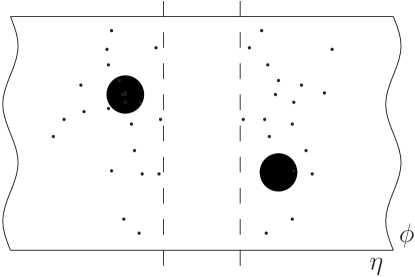
Figure 6.1: The experimental signature of a “jet-gap-jet” event. The dark circles denote two jets, and the gap region is bounded by the dashed lines.

The more recent H1 and ZEUS analyses used the kt definition of the final state and both collaborations presented the gap fraction at four different values of $Q_{\Omega}$, as shown in table 6.1. We will make predictions and compare to data for the H1 data sets and, due to the fact that the ZEUS data is still preliminary, confine ourselves to making predictions for the ZEUS analysis. We have summarised the cuts used in table 6.1.

	H1	ZEUS
$E_{T}^{\mathrm{jet1}}$	$>6.0$ GeV	$>6.0$ GeV
$E_{T}^{\mathrm{jet2}}$	$>5.0$ GeV	$>5.0$ GeV
$\eta^{\mathrm{jet1}}$	$<2.65$	$<2.4$
$\eta^{\mathrm{jet2}}$	$<2.65$	$<2.4$
$\Delta\eta$	$2.5<\Delta\eta<4$	$2<\Delta\eta<4$
$\eta_{\mathrm{jj}}$	N/A	$<0.75$
$y$	$0.3<y<0.6$	$0.2<y<0.85$
$Q^{2}$	$<0.01$ GeV2	$<1$ GeV2
jet def.	kt	kt
gap def.	$\Delta y=\Delta\eta$	$\Delta y=\Delta\eta$
$R$	$1.0$	$1.0$
$Q_{\Omega}$	$0.5,1.0,1.5,2.0$ GeV	$0.5,1.0,1.5,2.0$ GeV

Table 6.1: The experimental cuts used for the HERA analyses.

6.2.1 The kt algorithm

Of special interest to those going about soft gluon calculations is the method used to define the hadronic final state, the reason being that this jet-finding process determines the phase space for soft gluon emission; the method used in the H1 and ZEUS data sets is the kt algorithm [64, 65, 66]. Here we follow the inclusive scheme used at H1 and ZEUS which depends on the parameter R, normally set to unity. If we assume that any radiation into the gap is much softer than any parent radiation, then this radiation with $E_{T}<E_{T}^{\mathrm{jet}}$ will be merged into the jet (with kinematical variables $(\eta_{\mathrm{jet}},\phi_{\mathrm{jet}})$) if it satisfies

$$(\eta_{r}-\eta_{\mathrm{jet}})^{2}+(\phi_{r}-\phi_{\mathrm{jet}})^{2}<R^{2},$$ (6.1)

where we denote the kinematical variables of the radiated gluon by $(\eta_{r},\phi_{r})$. Once merged, a gluon will be pulled out of the gap and can no longer produce a primary or secondary logarithm. The gap is defined as the interjet region minus the region of clustered radiation around the jets and may contain soft protojets. The gap transverse energy is then defined by the (scalar) sum of the protojets within the gap region, $\eta_{1}<\eta<\eta_{2}$. We have given a detailed description of how the kt algorithm works in chapter 5.

The kt gap definition can be contrasted to the older ZEUS analysis [80], which used the well known cone definition of the final state with $R=1.0$. The gap transverse energy is then defined as the scalar sum of the transverse energy of the hadrons within it, $\eta_{1}+R<\eta<\eta_{2}-R$.

6.3 Factorisation, refactorisation and resummation of the cross section

In this section we will exploit the standard factorisation theorems of QCD to write down the dijet production cross section from the interaction of a proton and a positron. We will then refactorise the hard scattering function into the product of two matrices in the space of possible hard scattering colour flows, one matrix describing soft gluons radiated into the gap region and the other a hard scattering matrix. The renormalisation properties of the cross section are then used to resum primary interjet logarithms, and write the result in terms of the eigenvalues of the matrix of counterterms used to renormalise the soft function. In the following section we will calculate these matrices and their eigenvalues.

6.3.1 Photoproduction cross sections

The scattering of positrons and protons at HERA proceeds predominantly through the exchange of photons with very small virtuality and produces a large subset of events with jets of high transverse momentum, $E_{T}$. The presence of this large scale allows the application of the perturbative methods of QCD to predict the cross section for multiple jet production. This process is otherwise known as jet photoproduction.

The leading order (LO) QCD contribution can be divided into two types [59]. The first is the direct process in which the photon interacts directly with a parton from the proton and proceeds through either the Compton process, $\gamma q\rightarrow gq$, or the photon-gluon fusion process, $\gamma g\rightarrow q\bar{q}$. The second contribution is the resolved contribution, in which the virtual photon fluctuates into a hadronic state that acts as a source of partons, which then scatter off the partonic content of the proton. Therefore the reaction proceeds through standard QCD $2\rightarrow 2$ parton scattering processes. Note that the precise determination of the partonic content of the photon is a very open question and there is a relatively large error associated with the photonic parton densities. The spectrum of virtual photons is approximated by the Weizäcker–Williams [82] formula,

$$F_{\gamma/e}(y)=\frac{\alpha}{2\pi}\frac{(1+(1-y)^{2})}{y}\log\left(\frac{Q^{2}_{\mathrm{max}}(1-y)}{m_{e}^{2}y^{2}}\right),$$ (6.2)

where $m_{e}$ is the electron mass, $y$ is the fraction of the positron’s energy that is transfered to the photon, and $Q^{2}_{\mathrm{max}}$ is the maximum virtuality of the photon, which is determined by the experimental cuts employed in the analyses. Then, by using the equivalent photon approximation, the cross section for the process $e^{+}p\rightarrow e^{+}X$ is given by the convolution

$$\mathrm{d}\sigma(e^{+}p\rightarrow e^{+}X)=\int_{y_{\mathrm{min}}}^{y_{\mathrm{max}}}\mathrm{d}y\,F_{\gamma/e}(y)\,\mathrm{d}\sigma(\gamma p\rightarrow X),$$ (6.3)

where we write $\mathrm{d}\sigma(\gamma p\rightarrow X)$ for the cross section of $\gamma p\rightarrow X$. The centre of mass energy squared for the photon-proton system is $W^{2}=ys$, where $s$ is the centre of mass energy squared for the positron-proton system. At HERA, $s\simeq 90,000$ GeV² and the values for $y_{\mathrm{min}}$ and $y_{\mathrm{max}}$ are determined by the experimental analyses. We can now write down the specific expression for the production of two high $E_{T}$ jets from the photon-proton system, which is written as a sum of the direct and resolved contributions,

$$d\sigma_{e^{+}p}(s,\hat{t},\Delta\eta,\alpha_{s}(\mu_{r}),Q_{\Omega})= \int_{y_{min}}^{y_{max}}\mathrm{d}y\,F_{\gamma/e}(y)\bigg{(}\mathrm{d}\sigma_{\gamma p}^{\mathrm{dir}}(s_{\gamma p},\hat{t},\Delta\eta,\alpha_{s}(\mu_{r}),Q_{\Omega})$$ (6.4)

$$+\mathrm{d}\sigma_{\gamma p}^{\mathrm{res}}(s_{\gamma p},\hat{t},\Delta\eta,\alpha_{s}(\mu_{r}),Q_{\Omega})\bigg{)},$$

where we denote the 4-momentum transfer squared in the hard scattering as $\hat{t}$ and have temporarily suppressed the function arguments on the right-hand side. We define the rapidity difference and average of the two hard jets by

$$\Delta\eta = |\eta_{1}-\eta_{2}|,$$

$$\eta_{JJ} = \frac{1}{2}(\eta_{1}+\eta_{2}).$$ (6.5)

At this point we can appeal to the factorisation theorems of QCD and, by working in the $\gamma p$ frame, write down factorised forms for the direct and resolved cross sections. The factorised direct cross section is

$$\frac{\mathrm{d}\sigma_{\gamma p}^{\mathrm{dir}}}{\mathrm{d}\hat{\eta}}(s_{\gamma p},\hat{t},\Delta\eta,\alpha_{s}(\mu_{r}),Q_{\Omega})= \sum_{f_{p},f_{1},f_{2}}\int_{\mathrm{R_{d}}}\mathrm{d}x_{p}\,\phi_{f_{p}/p}(x_{p},\mu_{f})$$ (6.6)

$$\times\frac{\mathrm{d}\hat{\sigma}^{(\gamma f)}}{\mathrm{d}\hat{\eta}}(\hat{s},\hat{t},\Delta\eta,\alpha_{s}(\mu_{r}),Q_{\Omega},\mu_{f}),$$

and the factorised resolved cross section is

$$\frac{\mathrm{d}\sigma_{\gamma p}^{\mathrm{res}}}{\mathrm{d}\hat{\eta}}(s_{\gamma p},\hat{t},\Delta\eta,\alpha_{s}(\mu_{r}),Q_{\Omega})= \sum_{f_{\gamma},f_{p},f_{1},f_{2}}\int_{\mathrm{R_{r}}}\mathrm{d}x_{\gamma}\,\mathrm{d}x_{p}\,\phi_{f_{\gamma}/\gamma}(x_{\gamma},\mu_{f})\phi_{f_{p}/p}(x_{p},\mu_{f})$$ (6.7)

$$\times\frac{\mathrm{d}\hat{\sigma}^{(f)}}{\mathrm{d}\hat{\eta}}(\hat{s},\hat{t},\Delta\eta,\alpha_{s}(\mu_{r}),Q_{\Omega},\mu_{f})$$

which are written in terms of the jet rapidity, $\hat{\eta}$, in the partonic centre-of-mass frame, and we write the factorisation scale and the renormalisation scale as $\mu_{f}$ and $\mu_{r}$ respectively. Note that $\hat{\eta}=\Delta\eta/2$, $\hat{s}=x_{p}W^{2}$ for the direct case and $\hat{s}=x_{\gamma}x_{p}W^{2}$ for the resolved case. In these equations we denote the integration regions of the direct and resolved convolutions, which are defined by the experimental cuts, by ${\mathrm{R_{d}}}$ and ${\mathrm{R_{r}}}$. The parton distribution for a parton of flavour $f$ in the photon and the proton are denoted by $\phi_{f/\gamma}(x_{\gamma},\mu_{f})$ and $\phi_{f/p}(x_{p},\mu_{f})$ respectively and finally $\frac{\mathrm{d}\hat{\sigma}^{(\gamma f)}}{\mathrm{d}\hat{\eta}}$ and $\frac{\mathrm{d}\hat{\sigma}^{(f)}}{\mathrm{d}\hat{\eta}}$ are the hard scattering functions which, at lowest order, start from the Born cross sections. These are the functions that will contain the logarithmic enhancements of $Q_{\Omega}/Q$, and hence depend on the definition of the gap $\Omega$ and the gap energy flow $Q_{\Omega}$. We assume that $Q_{\Omega}$ is sufficiently soft that we can ignore the effects of emission on the parent jet, known as recoil, but large enough so that $Q_{\Omega}^{2}\gg\Lambda_{QCD}^{2}$. The index $f$ denotes the process $f_{\gamma}+f_{p}\rightarrow f_{1}+f_{2}$ and the index $f\gamma$ denotes the process $\gamma+f_{p}\rightarrow f_{1}+f_{2}$. Since the aim of this chapter is to calculate ratios of cross sections and compare with data, we will take the renormalisation scale to equal the factorisation scale and set $\mu_{f}=\mu_{r}=p_{t}$, where $p_{t}$ is the transverse momentum of the produced jets.

6.3.2 Refactorisation

Following [55, 7], and the arguments in chapter 4, we now refactorise the $2\rightarrow 2$ hard scattering function into a hard matrix and a soft matrix,

$$\frac{d\hat{\sigma}^{(f)}}{d\hat{\eta}}(\hat{s},\hat{t},\Delta\eta,\alpha_{s}(\mu_{r}),Q_{\Omega},\mu_{f})= \sum_{L,I}H^{(f)}_{IL}(\hat{s},\hat{t},\Delta\eta,\alpha_{s}(\mu_{r}),\mu_{f},\mu)$$ (6.8)

$$\times S^{(f)}_{LI}(Q_{\Omega},\alpha_{s}(\mu_{r}),\mu).$$

We introduce a factorisation scale $\mu$, separate to the parton distribution factorisation scale $\mu_{f}$, and all dynamics at scales less than $\mu$ are factored into $S_{LI}$. Therefore $H_{IL}$ is $Q_{\Omega}$ independent, and all the $Q_{\Omega}$ dependence is included in $S_{LI}$. This latter function describes the soft gluon dynamics. The proof of this statement follows standard factorisation arguments [7]. The indices $I$ and $L$ label the basis of colour tensors which describe the possible colour exchange in the hard scattering, over which the hard and soft matrices are expressed. Soft, wide angle radiation decouples from the dynamics of the hard scattering and can be approximated by an effective cross section and in this effective theory the partons are treated as recoilless sources of gluonic radiation and replaced by eikonal lines, or path ordered exponentials of the gluon field [53]. The soft radiation pattern of this effective eikonal theory then mimics the radiation pattern of the partons participating in the hard event, or in other words the effective eikonal theory will contain the same logarithms of the soft scale as the full theory. The hard scattering function will begin at order $\alpha_{s}^{2}$ for the resolved process and order $\alpha\alpha_{s}$ for the direct process, and the soft function will begin at zeroth order. The lowest order soft function, denoted $S^{0}_{LI}$, reduces to a set of colour traces. Note that the definition of the gap, and hence the soft function, depends on the jet separation $\Delta\eta$ but we have suppressed this argument of the soft function for clarity.

The construction of the soft function, and in particular its renormalisation properties, have been extensively studied elsewhere [53, 7], and are reviewed in chapter 4. A non-local operator is constructed from a product of Wilson lines, which ties four lines (representing the four jet process) together with a colour tensor. This operator, which contains ultraviolet divergences and hence requires renormalisation, is used to construct a so-called eikonal cross section, which serves as an effective theory for the soft emission. By summing over intermediate states the eikonal cross section is free of potential collinear singularities. It is the ultraviolet renormalisation of the eikonal operator that allows colour mixing and the resummation of soft interjet logarithms.

6.3.3 Factorisation leads to resummation of soft logarithms

The partonic cross section, which has been factorised into a hard and a soft function, should not depend on the choice of the factorisation scale $\mu$,

$$\mu\frac{\partial}{\partial\mu}\left(\frac{\mathrm{d}\hat{\sigma}}{\mathrm{d\hat{\eta}}}\right)=0.$$ (6.9)

Following chapter 4, this means the soft function obeys

$$\left(\mu\frac{\partial}{\partial\mu}+\beta(g_{s})\frac{\partial}{\partial g_{s}}\right)\uuline{S}=-\uuline{\Gamma_{s}}^{\dagger}(\hat{\eta},\Omega)\uuline{S}-\uuline{S}\uuline{\Gamma_{s}}(\hat{\eta},\Omega).$$ (6.10)

It is important to point out that we have deliberately ignored the complications of terms in this equation arising from radiation into $\bar{\Omega}$, as in [55] and chapter 4, and only include radiation emitted by the soft function directly into $\Omega$. The implication of ignoring these non-global terms is discussed in section 6.3.4, where we also describe how to include their effect in a different way. Therefore we have never included the, technically correct, $\bar{\Omega}$ argument of the soft function. The matrices $\Gamma_{s}(\hat{\eta},\Omega)$ are process-dependent soft anomalous dimension matrices which depend on the details of the gap definition and the hard scattering. This equation is solved by transforming to a basis in which these matrices are diagonal and hence we require a knowledge of the eigenvectors and eigenvalues of the soft anomalous dimension matrices. We obtain the entries for $\Gamma_{s}(\hat{\eta},\Omega)$ from the coefficients of the ultraviolet poles in the matrix of counterterms which renormalise the soft function; we can write the renormalisation constant as a sum over terms from different eikonal lines, each with the form of a colour factor multiplied by a scaleless integral:

$$(Z_{S})_{LI}=\sum_{i,j}(Z_{S}^{(ij)})_{LI}=\sum_{i,j}\mathcal{C}_{LI}^{(ij)}\omega^{(ij)}.$$ (6.11)

The eikonal momentum integrals are process independent, and only depend on $i$ and $j$, the eikonal lines that are connected by the virtual gluon. The colour factor is found from consideration of the colour flow for a given process and the basis over which the colour flow is to be decomposed. The result is a basis- and process-dependent set of colour mixing matrices, which we have listed in appendix F, together with our choice of bases in appendix D. The colour mixing matrices were discussed in detail in chapter 2 and have been obtained in [55, 9, 8] for all relevant subprocesses, and involves using SU(3) colour identities like

$$t^{a}_{ij}t^{a}_{kl}=\frac{1}{2}\delta_{il}\delta_{kj}-\frac{1}{2N_{c}}\delta_{ij}\delta_{kl},$$ (6.12)

for quark processes and

$$d_{abc} = 2\left[\mathrm{Tr}\left(t^{a}t^{c}t^{b}\right)+\mathrm{Tr}\left(t^{a}t^{b}t^{c}\right)\right],$$ (6.13)

$$f_{abc} = -2i\left[\mathrm{Tr}\left(t^{a}t^{b}t^{c}\right)-\mathrm{Tr}\left(t^{a}t^{c}t^{b}\right)\right],$$ (6.14)

for gluon processes, to decompose one-loop graphs over a colour basis. A more complete set of SU(3) group theoretic identities can be found in appendix A. We use the fact that the colour flow for a real graph is the same as the corresponding virtual graph, valid for primary emission.

Therefore we need to calculate the ultraviolet divergent contribution to the momentum function $\omega^{(ij)}$ from all contributing eikonal graphs. Working in the Feynman gauge there are two possible sources of divergence. The first is one loop eikonal graphs with a virtual gluon connecting eikonal lines $i$ and $j$. From the eikonal Feynman rules listed in the appendix, these graphs will give a real and an imaginary contribution to $\Gamma_{s}$. Note that as we are working in the Feynman gauge the self energy diagrams ($\omega^{(ii)}$) give no contribution. The second source of ultraviolet divergences are the real emission diagrams, when the emitted gluon is directed out of the gap. This can produce an ultraviolet divergence in the eikonal graph as we only measure energy flow into the gap and are fully inclusive out of the gap. Hence the virtual graphs will only depend on the relative direction of the two eikonal lines and the real graphs will give a gap (and hence a jet algorithm) dependence. This sum over real and virtual eikonal graphs ensures that the soft function remains free of collinear divergences. The imaginary (and geometry independent) part of all our anomalous dimension matrices can be extracted from [55, 58, 53, 8], and the calculation for a cone-algorithm defined final state has been done in [58]. For the latter case, we have re-expressed their results in accordance with our notation in appendix H.

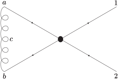
Figure 6.2: The virtual eikonal graph obtained if the virtual gluon connects eikonal lines $a$ and $b$. In the notation in the text, this diagram is denoted $I_{v}^{(ab)}$.

By performing the energy integral of the virtual graphs, we can combine the result with the corresponding real graph at the integrand level and obtain a partial cancellation. Therefore we start by evaluating a generic virtual eikonal graph, with the virtual gluon connecting eikonal lines $i$ and $j$, using the eikonal Feynman rules in appendix B. We obtain

$$I_{v}^{(ij)}=g_{s}^{2}\Delta_{i}\Delta_{j}\beta_{i}\cdot\beta_{j}\int\frac{d^{d}k}{(2\pi)^{d}}\frac{-i}{(k^{2}+i\epsilon)}\frac{1}{(\delta_{i}\beta_{i}\cdot k+i\epsilon)}\frac{1}{(\delta_{j}\beta_{j}\cdot k+i\epsilon)},$$ (6.15)

where $\delta_{i,j}=\pm 1$ and we denote the momenta of the virtual gluon by $k$. In this chapter we use the dimensional regularisation convention $d=4-2\epsilon$. Figure 6.2 shows the virtual eikonal diagram $I_{v}^{(ab)}$. Note that in this section we will use the symbol $\epsilon$ to denote a UV pole and also as a small parameter when doing contour integration. However there should be no confusion. Writing

$$d^{d}k = dk^{0}\,d^{d-1}\vec{k},$$ (6.16)

$$k^{\mu} = (k^{0},\vec{k}),$$ (6.17)

$$\beta_{i}^{\mu} = (1,\vec{\beta_{i}}),$$ (6.18)

$$k^{2}+i\epsilon = (k^{0}-|\vec{k}|+i\epsilon)(k^{0}+|\vec{k}|-i\epsilon),$$ (6.19)

we get

$$I_{v}^{(ij)}=g_{s}^{2}\Delta_{i}\Delta_{j}\beta_{i}\cdot\beta_{j}\int dk^{0}\frac{d^{d-1}\vec{k}}{(2\pi)^{d}}\frac{-i}{((k^{0})^{2}-\vec{k}^{2}+i\epsilon)}\frac{1}{(\delta_{i}[k^{0}-\vec{\beta_{i}}\cdot\vec{k}]+i\epsilon)}\frac{1}{(\delta_{j}[k^{0}-\vec{\beta_{j}}\cdot\vec{k}]+i\epsilon)}.$$ (6.20)

We need to evaluate the $k^{0}$ integral using contour integration, and there are four combinations of the $\delta_{i}^{\prime}s$ to consider; however the integrals only depend on the product $\delta_{i}\delta_{j}$ and so it is sufficient to only consider two of the four possible combinations of $\delta_{i}$ and $\delta_{j}$. The four poles in the complex $k^{0}$ plane are

$$k^{0} = -|\vec{k}|+i\epsilon,$$

$$k^{0} = +|\vec{k}|-i\epsilon,$$

$$k^{0} = (\delta_{i}\vec{\beta_{i}}\cdot\vec{k}-i\epsilon)/\delta_{i},$$

$$k^{0} = (\delta_{j}\vec{\beta_{j}}\cdot\vec{k}-i\epsilon)/\delta_{j}.$$ (6.21)

We consider the case of $\delta_{i}=\delta_{j}=-1$, for which the poles are

$$k^{0} = -|\vec{k}|+i\epsilon,$$

$$k^{0} = +|\vec{k}|-i\epsilon,$$

$$k^{0} = \vec{\beta_{i}}\cdot\vec{k}+i\epsilon,$$

$$k^{0} = \vec{\beta_{j}}\cdot\vec{k}+i\epsilon.$$ (6.22)

We close the contour in the lower-half plane and only pick up the pole $k^{0}=+|\vec{k}|-i\epsilon$. The residue of this pole is extracted from the standard result of the Laurent expansion

$$\dots+\frac{a_{-1}}{z-z_{o}}|_{z=z_{0}}+\dots$$ (6.23)

and we get for the residue (where we have used equation (6.19) to obtain the desired form)

$$a_{-1}=\frac{-i}{(2|\vec{k}|-i\epsilon)(-|\vec{k}|+\vec{\beta_{i}}\cdot\vec{k}+i\epsilon)(-|\vec{k}|+\vec{\beta_{j}}\cdot\vec{k}+i\epsilon)}.$$ (6.24)

Therefore, multiplying by $2\pi i$ and by $-1$ (for going clockwise around the contour), we get

$$I^{(\delta_{i}=\delta_{j}=-1)} = (-2\pi i)g_{s}^{2}\Delta_{i}\Delta_{j}\beta_{i}\cdot\beta_{j}\int\frac{d^{d-1}k}{(2\pi)^{d}}\frac{-i}{2|\vec{k}|(-\beta_{i}\cdot k)(-\beta_{j}\cdot k)},$$ (6.25)

$$= -g_{s}^{2}\Delta_{i}\Delta_{j}\beta_{i}\cdot\beta_{j}\int\frac{d^{d-1}k}{(2\pi)^{d-1}}\frac{1}{2|\vec{k}|(-\beta_{i}\cdot k)(-\beta_{j}\cdot k)},$$

as $\epsilon\rightarrow 0$. We note that this expression is the same as the real diagram expression integrated over all of phase space, and with an overall minus sign. This real diagram expression is readily obtained from the evaluation of an eikonal diagram with real gluon emission using the eikonal Feynman rules in appendix B. We can also see that, if we have no restrictions on the real gluon emission energy, we expect a complete cancellation of real and virtual diagrams. Now consider the case of $\delta_{i}=+1$ and $\delta_{j}=-1$. This configuration corresponds to virtual diagrams where the virtual gluon connects the incoming eikonal lines. Now we have the following arrangement of poles,

$$k^{0} = -|\vec{k}|+i\epsilon,$$

$$k^{0} = +|\vec{k}|-i\epsilon,$$

$$k^{0} = \vec{\beta_{i}}\cdot\vec{k}-i\epsilon,$$

$$k^{0} = \vec{\beta_{j}}\cdot\vec{k}+i\epsilon.$$ (6.26)

with two in the upper half plane, and two in the lower-half plane. We choose to close the contour in the lower-half plane again and pick up two poles. The residues are computed in exactly the same manner as the first case and we obtain, for the $k^{0}=+|\vec{k}|-i\epsilon$ pole

$$a_{-1}=\frac{-i}{(2|\vec{k}|-i\epsilon)}\frac{1}{(|\vec{k}|-\vec{\beta_{i}}\cdot\vec{k})}\frac{1}{(-|\vec{k}|+\vec{\beta_{j}}\cdot\vec{k}+i\epsilon)},$$ (6.27)

and for the $k^{0}=\vec{\beta_{i}}\cdot\vec{k}-i\epsilon$ pole

$$a_{-1}=\frac{-i}{((\vec{\beta_{i}}\cdot\vec{k}-i\epsilon)^{2}-\vec{k}^{2}+i\epsilon)(\vec{\beta_{j}}\cdot\vec{k}-\vec{\beta_{i}}\cdot\vec{k}+i\epsilon)}.$$ (6.28)

Note that to get the correct form of the first residue, we need to use the form of the integrand containing equation (6.19), and to get the correct form for the second residue we need to use the $k^{2}=(k^{0})^{2}-\vec{k}^{2}$ form of the integrand. Therefore the integral for this arrangement of poles has two contributions - one from the $k^{2}$ pole and another from the $\beta\cdot k$ pole. The first gives

$$I^{(\delta_{i}=+1,\delta_{j}=-1)}=-g_{s}^{2}\Delta_{i}\Delta_{j}\beta_{i}\cdot\beta_{j}\int\frac{d^{d-1}k}{(2\pi)^{d-1}}\frac{1}{2|\vec{k}|(\beta_{i}\cdot k)(-\beta_{j}\cdot k)},$$ (6.29)

and the latter gives

$$I_{s}=-g_{s}^{2}\beta_{i}\cdot\beta_{j}\int\frac{d^{d-1}k}{(2\pi)^{d-1}}\frac{1}{((\vec{\beta_{i}}\cdot\vec{k})^{2}-\vec{k}^{2}\pm i\epsilon)(\vec{\beta_{j}}\cdot\vec{k}-\vec{\beta_{i}}\cdot\vec{k}+i\epsilon)}.$$ (6.30)

We will give an explanation for the $s$ subscript later in this section. The $\pm$ piece comes from the unknown sign of $\vec{\beta_{i}}\cdot k$. Note that, once again, the piece arising from the $k^{2}$ poles gives a contribution looking like the negative of the real contribution. At first sight, it looks like the real diagrams should give a $\beta_{i}\cdot k$ pole if we write the Lorentz invariant phase space in 4 dimensions using

$$\int\frac{d^{3}p}{(2\pi)^{3}}=\int\frac{d^{4}p}{(2\pi)^{4}}(2\pi)\delta^{+}(p^{2}),$$ (6.31)

where we express the on-shell condition of real gluons as

$$\delta^{+}(p^{2})=\delta(p^{2})\Theta(p^{0}).$$ (6.32)

The $\beta_{i}\cdot k$ pole is not picked up by the real diagram energy integral, due to this condition. We have determined that if we perform the energy integral of a virtual eikonal graph, we obtain the same form as the corresponding (same $i$ and $j$) real graph. We shall not consider the analysis of the remaining pole configurations, for which we will draw the same conclusions, and describe how everything fits together. We are interested in the ultraviolet pole part of the real and virtual one-loop eikonal diagrams, in order to calculate the soft anomalous dimension matrix. The virtual loop diagrams contribute through their loop integrals and the real diagrams contribute in all regions where we are completely inclusive of gluonic radiation (everywhere except any “gap” region.) Therefore

$$\omega^{(ij)} = I_{v}^{(ij)}+I_{r}^{(ij)},$$ (6.33)

$$= g_{s}^{2}\Delta_{i}\Delta_{j}\beta_{i}\cdot\beta_{j}\int\frac{d^{d}k}{(2\pi)^{d}}\frac{-i}{(k^{2}+i\epsilon)}\frac{1}{(\delta_{i}\beta_{i}\cdot k+i\epsilon)}\frac{1}{(\delta_{j}\beta_{j}\cdot k+i\epsilon)}$$

$$+ g_{s}^{2}\Delta_{i}\Delta_{j}\beta_{i}\cdot\beta_{j}\int\frac{d^{d-1}k}{(2\pi)^{d-1}}(1-\Theta(\vec{k}))\frac{1}{2|\vec{k}|(\delta_{i}\beta_{i}\cdot k)(\delta_{j}\beta_{j}\cdot k)}.$$

In writing this line we have used the explicit forms of the virtual and real diagrams, with the virtual gluon joining eikonal lines $i$ and $j$. The function $\Theta(\vec{k})=1$ when the real gluon is directed into the gap, and is zero otherwise. We can now do the virtual $k^{0}$ integral,

$$\omega^{(ij)} = -g_{s}^{2}\Delta_{i}\Delta_{j}\beta_{i}\cdot\beta_{j}\int\frac{d^{d-1}k}{(2\pi)^{d-1}}\frac{1}{2|\vec{k}|(-\beta_{i}\cdot k)(-\beta_{j}\cdot k)},$$ (6.34)

$$+ g_{s}^{2}\Delta_{i}\Delta_{j}\beta_{i}\cdot\beta_{j}\int\frac{d^{d-1}k}{(2\pi)^{d-1}}(1-\Theta(\vec{k}))\frac{1}{2|\vec{k}|(\delta_{i}\beta_{i}\cdot k)(\delta_{j}\beta_{j}\cdot k)},$$

$$+ \frac{1}{2}I_{s}(1-\delta_{i}\delta_{j})$$

$$= -g_{s}^{2}\Delta_{i}\Delta_{k}\beta_{i}\cdot\beta_{j}\int\frac{d^{d-1}k}{(2\pi)^{d-1}}\Theta(\vec{k})\frac{1}{2|\vec{k}|(\delta_{i}\beta_{i}\cdot k)(\delta_{j}\beta_{j}\cdot k)}$$

$$+ \frac{1}{2}I_{s}(1-\delta_{i}\delta_{j}),$$

and find that its real part can be written as $-1\,\times$ the real contribution, but with no phase space restrictions. This part is the bit left over from picking up the $k^{2}$ pole. The function $I_{s}$ is the result of picking up the $\beta_{i}\cdot k$ pole, and is only present when $\delta_{i}=-1\times\delta_{j}$, or when the virtual gluon connects two initial or final state eikonal lines (s-channel diagrams). This is the reason for the $s$ subscript for the function $I_{s}$. We have also performed a real/virtual cancellation and have been left with an integral over the vetoed gap region, plus an additional function $I_{s}$, equation (6.30). To evaluate this latter piece we use polar coordinates in $(d-1)$ dimensions,

$$\mathrm{d}^{d-1}k=k^{d-2}\mathrm{d}k\,\,\mathrm{d}\cos{\theta}\,\,\mathrm{d}\phi\,\,\mathrm{d}^{d-4}\Omega,$$ (6.35)

where we have noted that this integral only appears in diagrams in which $\vec{\beta_{i}}$ and $\vec{\beta_{j}}$ are back-to-back (and so $\beta_{i}\cdot\beta_{j}=2$), and write

$$\vec{\beta_{i}}\cdot\vec{k} = k\cos\theta,$$ (6.36)

$$\vec{\beta_{j}}\cdot\vec{k} = -k\cos\theta.$$ (6.37)

Note that the a general polar d-vector for $k$ is

$$k^{\mu}=k(1;\dots,\sin\theta\sin\phi,\sin\theta\cos\phi,\cos\theta).$$ (6.38)

Doing this we obtain the integrand

$$\frac{1}{(\cos^{2}(\theta)-1\pm i\epsilon)(-2\cos(\theta)+i\epsilon)} = \frac{1}{(2\cos(\theta)-i\epsilon)(1\mp i\epsilon+1/4\epsilon^{2})}$$ (6.39)

$$+ \frac{(2\cos(\theta)+i\epsilon)}{(1-\cos^{2}(\theta)\mp i\epsilon)(4\mp 4i\epsilon+\epsilon^{2})},$$

where we have used partial fractions to write the second form. We can safely set $\epsilon=0$ in the second term, since the only poles present are at $\cos\theta=\pm 1$ and these are protected by dimensional regularisation. Therefore the second term is an odd function of $\cos\theta$ and integrates (over the range $-1$ to $+1$) to zero. Therefore we are left with

$$\int_{-1}^{+1}\frac{d\cos(\theta)}{2\cos(\theta)-i\epsilon}=+\frac{\pi}{2}i-\mathcal{O}(\epsilon),$$ (6.40)

Hence we find that the imaginary piece is

$$I_{s} = -\frac{g_{s}^{2}}{(2\pi)^{2}}\frac{1}{2\epsilon}2\Delta_{i}\Delta_{j}\frac{\pi}{2}{i},$$ (6.41)

$$= \Delta_{i}\Delta_{j}\delta_{i}\delta_{j}\frac{\alpha_{s}}{\pi}\frac{i\pi}{2\epsilon},$$ (6.42)

where we have used the fact that

$$\int_{\mathrm{PP}}\frac{k^{d-2}dk}{k^{3}}=\frac{1}{2\epsilon},$$ (6.43)

for $d=4-2\epsilon$ and an integration from some fixed energy to infinity. Therefore the momentum integrals take the form,

$$\omega^{(ij)} = I_{v}^{(ij)}+I_{r}^{(ij)},$$ (6.44)

$$= -g_{s}^{2}\Delta_{i}\Delta_{k}\beta_{i}\cdot\beta_{j}\int\frac{d^{d-1}k}{2|\vec{k}|(2\pi)^{d-1}}\Theta(\vec{k})\frac{1}{(\delta_{i}\beta_{i}\cdot k)(\delta_{j}\beta_{j}\cdot k)},$$

$$+ \delta_{i}\delta_{j}\Delta_{i}\Delta_{j}\frac{\alpha_{s}}{2\pi}\frac{i\pi}{2\epsilon}(1-\delta_{i}\delta_{j}),$$

which we can write in terms of the rapidity and transverse energy of the emitted gluon,

$$\omega^{(ij)}=-\frac{g_{s}^{2}}{2}\Delta_{i}\Delta_{j}\delta_{i}\delta_{j}\frac{1}{(2\pi)^{2}}\int k_{t}\,dk_{t}\,d\eta\,\frac{d\phi}{2\pi}\Theta(\vec{k})\frac{\beta_{i}\cdot\beta_{j}}{(\beta_{i}\cdot k)(\beta_{j}\cdot k)}+I.P..$$ (6.45)

We have written the geometry independent imaginary part as I.P.. Once we have obtained the momentum integrals for the kt defined final state we can construct the anomalous dimension matrices using the colour mixing matrices in appendix F. Consideration of the eigenvalues and eigenvectors of these matrices, together with the process-dependent hard and soft matrices (the full set of hard and soft matrices is shown in appendix E ) allows the resummed cross section to be written down,

$$\frac{d\hat{\sigma}^{(f)}}{d\hat{\eta}}=\sum_{L,I}\bar{H}^{0,(f)}_{IL}\bar{S}^{0,(f)}_{LI}\exp\left\{\frac{1}{\beta_{0}}(\hat{\lambda}_{L}^{*}(\hat{\eta},\Omega)+\hat{\lambda}_{I}(\hat{\eta},\Omega))\int_{p_{t}}^{Q_{\Omega}}\frac{d\mu}{\mu}\beta_{0}\alpha_{s}(\mu)\right\},$$ (6.46)

which follows from the diagonalisation of the soft RGE, equation (6.10). This was discussed in chapter 4, where we developed this resummed expression from the factorisation properties of the cross section. We denote matrices in the diagonal basis by barred matrices, the eigenvalues of the anomalous dimension matrices by $\lambda_{i}=\alpha_{s}\hat{\lambda}_{i}$ and we write the lowest-order piece of the QCD beta function as $\beta_{0}=(11N_{c}-2n_{f})/(6\pi)$. Note that our normalisation of the eigenvalues differs by a factor of $\pi$ from that used in chapter 4. We will observe that, in agreement with [58], $\mathrm{Re}(\lambda)>0$ for all physical channels and hence the resummed cross sections are suppressed relative to the fully inclusive cross section.

6.3.4 Non-global effects

As we have discussed in the last section, we have deliberately ignored terms arising from secondary radiation into $\Omega$, or non-global logarithms (NGLs) [71, 70, 61, 60]. Such terms arise from radiation at some intermediate scale, $M$, being emitted outside of $\Omega$, i.e. into $\bar{\Omega}$, and then subsequently radiating into $\Omega$. In energy flow observables such effects give rise to leading logarithms. Inclusion of NGLs in the formalism of the last section would result in an explicit $M$ dependence of the soft function and a sensitivity to more complicated, $2\rightarrow n$, colour flows for all $n>2$. For further details see [55]. NG effects have been studied for a two-jet system by Dasgupta and Salam [61, 60], by Appleby and Seymour with the complication of clustering [70], and in the context of energy flow/event shape correlations by Dokshitzer and Marchesini [76] and Berger, Kúcs and Sterman [75].

The effect of NGLs for four-jet kinematics has not been explicitly calculated to date. The best that has been managed is a two-jet calculation in the large-$N_{c}$ limit. The NG contributions to the gap cross section factorize into an overall suppression factor $S^{NG}$, making it smaller than would be predicted by the resummation of primary logarithms alone. In the absence of a complete calculation, we include the NGLs approximately, by using our all-order results in the large-$N_{c}$ limit for $S^{NG}$ in a two-jet system [70]. Since four-jet configurations are dominated, in the large-$N_{c}$ limit and for large $\Delta\eta$, by colour flows in which two colour dipoles stretch across the gap region, we approximate the four-jet NG suppression factor by the square of the two-jet one.

We have reperformed our previous calculation for the kinematic range relevant to HERA and find that the variation of $S^{NG}$ with $\Delta\eta$ is very weak, so we neglect it. The variation with $Q_{\Omega}$ is very strong on the other hand. $S^{NG}$ is a function of $t$,

$$t=\frac{1}{2\pi\beta_{0}}\log\left(\frac{\alpha_{s}(Q_{\Omega})}{\alpha_{s}(Q)}\right),$$ (6.47)

where $\beta_{0}=(11C_{A}-2n_{f})/(6\pi)$, and is well-approximated by a Gaussian in $t$. Thus if $Q_{\Omega}$ is too close to $\Lambda_{QCD}$, $t$ varies rapidly with it and $S^{NG}$ varies very rapidly.

$Q_{\Omega}$ [GeV]	$S^{NG}(t)^{2}$
0.5	0.10${}^{+0.30}_{-0.10}$
1.0	0.47${}^{+0.16}_{-0.22}$
1.5	0.65${}^{+0.10}_{-0.13}$
2.0	0.74${}^{+0.07}_{-0.08}$

Table 6.2: The non-global emission suppression factors for the 4-jet system, obtained from an all-orders calculation for $Q=6$ GeV.

It is impossible to quantify the uncertainties in this approximation, without a more detailed understanding of the underlying physics. To get an idea however, we estimate the possible size of higher order corrections, by varying the hard scale at which $\alpha_{s}$ is evaluated. To leading logarithmic accuracy, this is equivalent to varying the value of $\alpha_{s}(Q)$ by an amount proportional to its value. Therefore we estimate the uncertainty by

$$\alpha_{s}^{\mathrm{up}} = \alpha_{s}(1+\alpha_{s}),$$ (6.48)

$$\alpha_{s}^{\mathrm{down}} = \alpha_{s}(1-\alpha_{s}).$$ (6.49)

We therefore evaluate $t$, and hence $S^{NG}(t)^{2}$, using our central value of $\alpha_{s}(M_{z})=0.116$, which implies $\alpha_{s}(Q=\mbox{6~{}GeV})=0.196$, and with raised and lowered values $\alpha_{s}^{\mathrm{up}}(\mbox{6~{}GeV})=0.234$ and $\alpha_{s}^{\mathrm{down}}(\mbox{6~{}GeV})=0.158$. For $Q_{\Omega}=1.0$ GeV, for example, these values result in $t=0.097^{+0.056}_{-0.032}$ and hence $S^{NG}(t)^{2}=0.47^{+0.16}_{-0.22}$. We show the results for all relevant values of $Q_{\Omega}$ in table 6.2. Note that $Q_{\Omega}=0.5$ GeV is so low that the range of uncertainty in $t$ extends beyond $\Lambda_{QCD}$ and hence the estimate of $S^{NG}$ extends to zero. We have not shown any results for the 1995 cone-based ZEUS energy flow analysis [80] because the low value of $Q_{\Omega}=0.3$ GeV means that the central value of the NG suppression is already zero, indicating a breakdown of our perturbative approach.

The uncertainty on the secondary emission probability estimated in this way should be added to that on the primary emission probability, described in section 6.5. However, we will see that the secondary uncertainty generally dominates the two. This is therefore clearly an area that needs more work if more precise quantitative predictions are to be made.

6.4 Soft gluon dynamics for a kt defined final state

We now evaluate the momentum integral, $\omega^{(ij)}$, over the gap region $\Omega$. The region of integration is determined by the experimental geometry, in which the final state is defined by the kt algorithm, and we shall work with the quantity

$$\Omega_{kt}^{(ij)}=\int_{kt}\mathrm{d}\eta\int_{kt}\frac{\mathrm{d}\phi}{2\pi}\frac{\beta_{i}\cdot\beta_{j}}{(\beta_{i}\cdot\bar{k})(\beta_{j}\cdot\bar{k})},$$ (6.50)

where we define $\bar{k}=k/k_{t}$. Therefore

$$\omega^{(ij)}=-\frac{\alpha_{s}}{2\pi}\Delta_{i}\Delta_{j}\delta_{i}\delta_{j}\frac{1}{2\epsilon}\Omega_{kt}^{(ij)}+I.P..$$ (6.51)

We denote the geometry independent imaginary part by $I.P.$, and we define the finite piece $\Gamma^{(ij)}$ by

$$\omega^{(ij)}=-\mathcal{S}_{ij}\frac{\Gamma^{(ij)}}{2\epsilon}.$$ (6.52)

We have extracted the sign function from $\Gamma^{(ij)}$,

$$\mathcal{S}_{ij}=\Delta_{i}\Delta_{j}\delta_{i}\delta_{j},$$ (6.53)

so that

$$\Gamma^{(ij)}=\frac{\alpha_{s}}{2\pi}\Omega^{(ij)}_{kt}+I.P..$$ (6.54)

In this work we denote the rapidity separation of the jets by $\Delta\eta$ and the width of an azimuthally symmetric rapidity gap by $\Delta y$ ($<\Delta\eta$). Therefore the available phase space for soft gluon emission for a kt defined final state is given by

$$\Omega_{kt}^{(ij)}=\lim_{\Delta y\rightarrow\Delta\eta}\left(\Omega^{(ij)}_{f}(\Delta y,\Delta\eta)-\Omega^{(ij)}_{1}(\Delta y,\Delta\eta,R)-\Omega^{(ij)}_{2}(\Delta y,\Delta\eta,R)\right),$$ (6.55)

where the first term arises from an azimuthally symmetric gap of width $\Delta y$, and we subtract the region around each jet which is vetoed by the kt algorithm. The regions of this equation are shown in figure 6.3.

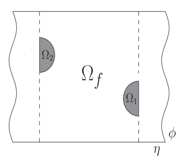
Figure 6.3: The phase space regions for a kt defined final state. The shading denotes the regions vetoed by the algorithm, which are subtracted from the $\Omega_{f}$ piece. Note that we have dropped the ${(ij)}$ superscripts in this figure.

In these regions any soft radiation is clustered into the jet, and cannot form part of $\Omega$. In the first term we take $\Delta y$ approaching $\Delta\eta$, and hence it contains a collinear divergence when the emitted gluon is collinear to one of the jets. The two subtracted pieces then remove the regions of phase space defined by

$$(\eta_{k}-\eta_{i})^{2}+(\phi_{k}-\phi_{i})^{2}<R^{2},$$ (6.56)

where the index $i$ labels final state jets and $k$ labels the emitted gluon. The collinear divergences in the subtracted pieces exactly match the divergences in the first piece and hence the function $\Omega^{(ij)}_{kt}(\Delta\eta)$ is collinear safe. Explicit definitions of the $\Omega$ functions are

$$\Omega^{(ij)}_{f} = \int_{-\Delta y/2}^{+\Delta_{y}/2}\mathrm{d}\eta\int_{0}^{2\pi}\frac{\mathrm{d}\phi}{2\pi}\frac{\beta_{i}\cdot\beta_{j}}{(\beta_{i}\cdot\bar{k})(\beta_{j}\cdot\bar{k})},$$

$$\Omega^{(ij)}_{1} = \int_{\Delta\eta/2-R}^{+\Delta y/2}\mathrm{d}\eta\int_{-\phi_{\mathrm{lim}}}^{+\phi_{\mathrm{lim}}}\mathrm{d}\phi\frac{\beta_{i}\cdot\beta_{j}}{(\beta_{i}\cdot\bar{k})(\beta_{j}\cdot\bar{k})},$$ (6.57)

where we write $\phi_{\mathrm{lim}}=\sqrt{R^{2}-(\eta-\Delta\eta/2)^{2}}$ and obtain $\Omega^{(ij)}_{2}$ by the symmetry $\Omega^{(ij)}_{2}=\Omega^{(\bar{\imath}\bar{\jmath})}_{1}$, where the mapping $i\to\bar{\imath}$ is given by $\{a,b,1,2\}\to\{b,a,2,1\}$. If we define the following combinations of momentum integrals,

$$\alpha = \mathcal{S}_{ab}\Gamma^{(ab)}+\mathcal{S}_{12}\Gamma^{(12)},$$

$$\beta = \mathcal{S}_{a1}\Gamma^{(a1)}+\mathcal{S}_{b2}\Gamma^{(b2)},$$

$$\gamma = \mathcal{S}_{b1}\Gamma^{(b1)}+\mathcal{S}_{a2}\Gamma^{(a2)},$$ (6.58)

where we have combined classes of diagram with the same colour structure, we obtain the following closed form for the positive gap contributions, in the limit $\Delta y\rightarrow\Delta\eta$,

$$\alpha = \frac{\alpha_{s}}{\pi}\Bigl{(}\phantom{-}2\Delta\eta+\log\bigl{(}1-e^{-2\Delta\eta}\bigr{)}+\log\frac{1}{\Delta\eta-\Delta y}-2i\pi\Bigr{)},\phantom{(10)}$$ (6.59)

$$\beta = \frac{\alpha_{s}}{\pi}\Bigl{(}\phantom{-2\Delta\eta+{}}\log\bigl{(}1-e^{-2\Delta\eta}\bigr{)}+\log\frac{1}{\Delta\eta-\Delta y}\Bigr{)},$$ (6.60)

$$\gamma = \frac{\alpha_{s}}{\pi}\Bigl{(}-2\Delta\eta-\log\bigl{(}1-e^{-2\Delta\eta}\bigr{)}-\log\frac{1}{\Delta\eta-\Delta y}\Bigr{)}.$$ (6.61)

The subtraction pieces are straightforward to express as power series in $R$ and $e^{-\Delta\eta}$ and we shall illustrate the calculation of the momentum integrals with an example.

6.4.1 Calculation of $\Omega_{kt}^{(a1)}$

We can write the matrix element in terms of the rapidity of the emitted gluon and obtain the following matrix element

$$\frac{\beta_{a}\cdot\beta_{1}}{(\beta_{a}\cdot\bar{k})(\beta_{1}\cdot\bar{k})}=\frac{e^{-\Delta\eta/2}}{e^{-\eta}(\cosh(\Delta\eta/2-\eta)-\cos\phi)},$$ (6.62)

using the 4-momenta products,

$$\beta_{a}\cdot\beta_{1} = \cosh(\Delta\eta/2)-\sinh(\Delta\eta/2),$$ (6.63)

$$\beta_{a}\cdot\bar{k} = \cosh(\eta/2)-\sinh(\eta/2),$$ (6.64)

$$\beta_{1}\cdot\bar{k} = \cosh(\Delta\eta/2)\cosh\eta-\sinh(\Delta\eta/2)\sinh\eta-\cos\phi.$$ (6.65)

The integrations for the function $\Omega_{f}^{(a1)}$ are straightforward, and we obtain

$$\Omega_{f}^{(a1)}=-\Delta y+\log\left(\frac{\sinh(\Delta\eta/2+\Delta y/2)}{\sinh(\Delta\eta/2-\Delta y/2)}\right).$$ (6.66)

The expression for $\Omega_{1}^{(a1)}$ is

$$\Omega^{(a1)}_{1} = \int_{\Delta\eta/2-R}^{+\Delta y/2}\mathrm{d}\eta\int_{-\phi_{\mathrm{lim}}}^{+\phi_{\mathrm{lim}}}\frac{\mathrm{d}\phi}{2\pi}\frac{e^{-\Delta\eta/2}}{e^{-\eta}(\cosh(\Delta\eta/2-\eta)-\cos\phi)},$$ (6.67)

$$= \int_{\Delta\eta/2-R}^{+\Delta y/2}\mathrm{d}\eta\,f(\eta,\Delta\eta,R),$$

$$= \int_{\Delta\eta/2-\Delta y/2}^{R}\mathrm{d}\eta^{\prime}\,f(\eta^{\prime},\Delta\eta,R),$$

where $\phi_{\mathrm{lim}}$ is defined in the previous section, we have performed the azimuthal integration in the second step and changed variable to $\eta^{\prime}=\Delta\eta/2-\eta$ in the third step. The function $f$ can be easily obtained, but it is rather lengthy so we do not reproduce it here. We now note that this expression for $\Omega^{(ij)}_{1}$ only involves jet 1 and hence, by Lorentz invariance, cannot depend on the other jet and so may not be a function of the jet separation $\Delta\eta$. Therefore we write

$$\Omega^{(a1)}_{1}=\int_{\Delta\eta/2-\Delta y/2}^{R}\mathrm{d}\eta^{\prime}\,f(\eta^{\prime},R).$$ (6.68)

This function $f(\eta^{\prime},R)$ has a divergence as $\eta^{\prime}\rightarrow 0$, so we add and subtract this divergence to obtain

$$\Omega^{(a1)}_{1}=\int_{\Delta\eta/2-\Delta y/2}^{R}\mathrm{d}\eta^{\prime}\left(f(\eta^{\prime},R)-\frac{1}{\eta^{\prime}}\right)+\int_{\Delta\eta/2-\Delta y/2}^{R}\frac{\mathrm{d}\eta^{\prime}}{\eta^{\prime}}.$$ (6.69)

We can rewrite the lower limit of the first, divergence free, integral as 0, and the collinear divergence is now contained in the second term. Therefore we have used $\Delta y$ as a cut-off for the divergence, and we can write

$$\Omega^{(a1)}_{1}=\bar{\Omega}^{(a1)}_{1}+\log{2R}-\log(\Delta\eta-\Delta y)+\mathcal{O}(\Delta\eta-\Delta y).$$ (6.70)

We will always denote the divergence free angular integrals, which result from such subtractions, as barred quantities. We can now rescale the $\bar{\Omega}^{(a1)}_{1}$ integral, using

$$\bar{\eta}=\eta^{\prime}/R,$$ (6.71)

to obtain

$$\bar{\Omega}^{(a1)}_{1}=\int_{0}^{1}\mathrm{d}\bar{\eta}\left(R\cdot g(\bar{\eta},R)-\frac{1}{\bar{\eta}}\right).$$ (6.72)

We have denoted the rescaled version of $f$ by $g$. This quantity, which is only a function of $R$, can now be expressed as a power series in $R$ and the integrals done on a term-by-term basis. Doing this we obtain the rapidly converging series,

$$\bar{\Omega}^{(a1)}_{1}=-\log(2)-\frac{2R}{\pi}+\frac{R^{2}}{8}-\frac{R^{3}}{18\pi}+\frac{R^{4}}{576}-\frac{R^{5}}{5400\pi}-\frac{R^{7}}{529200\pi}+\frac{R^{8}}{4147200}+\dots.$$ (6.73)

To calculate $\Omega^{(a1)}_{2}$ we use the parity symmetry mapping, $\{a,b,1,2\}\to\{b,a,2,1\}$, and obtain the expression,

$$\Omega^{(a1)}_{2} = \Omega^{(b2)}_{1}$$ (6.74)

$$= \int_{\Delta\eta/2-R}^{+\Delta y/2}\mathrm{d}\eta\int_{-\phi_{\mathrm{lim}}}^{+\phi_{\mathrm{lim}}}\frac{\mathrm{d}\phi}{2\pi}\frac{e^{-\Delta\eta/2}}{e^{\eta}(\cosh(\Delta\eta/2+\eta)+\cos\phi)}.$$

We now perform similar manipulations to the case of $\Omega^{(a1)}_{1}$. However, as $\Omega^{(a1)}_{2}$ is a function of both final state jets, the resulting expression must be a function of $\Delta\eta$ and we also note that $\Omega^{(a1)}_{2}$ is not divergent. We hence obtain the expression

$$\bar{\Omega}_{2}^{(a1)}=\int_{0}^{1}d\bar{\eta}\left(R\cdot f(\bar{\eta},\Delta\eta,R)\right),$$ (6.75)

which we can expand as a power series in the variables $R$ and $z=\exp(-\Delta\eta)$, and perform the remaining integrations term-by-term.

The pole arising in the subtraction term $\Omega_{1}^{(a1)}$ now cancels against an equivalent pole in the function $\Omega_{f}^{(a1)}$, when we expand the latter in $\Delta y$ around the point $\Delta\eta$,

$$\lim_{\Delta y\rightarrow\Delta\eta}\Omega_{f}^{(a1)}\sim-\Delta\eta-\log(\Delta\eta-\Delta y)+\log(2\sinh\Delta\eta).$$ (6.76)

Therefore we find the final, divergence free, form of $\Omega_{kt}^{(a1)}$ as

$$\Omega_{kt}^{(a1)}=-\Delta\eta+\log(2\sinh\Delta\eta)-\log(2R)-\bar{\Omega}_{1}^{(a1)}-\bar{\Omega}_{2}^{(a1)}.$$ (6.77)

We have presented the full set of series expansions in appendix G and these, together with equations (6.59–6.61), are sufficient to compute the set of kt defined momentum integrals and hence the corresponding anomalous dimension matrix. It is worth noting that, although the off-diagonal terms for the kt anomalous dimension matrices are no longer pure imaginary, as in the cone case, their real parts still vanish for large $\Delta\eta$. Indeed for $\Delta\eta=2$, the real part is more than two orders of magnitude smaller than the imaginary part. We have listed the closed-form momentum integrals for the cone defined final state using our notation in appendix H.

6.5 Results

We now have the tools we need to calculate resummed cross sections at HERA, which correctly include primary emission to all orders and secondary emission approximately in the large $N_{c}$ limit. The colour bases used for the contributing partonic cross sections are presented in the appendix, along with the decomposed hard and soft matrices. We also present the complete colour mixing matrices and the correct sign structure for the three classes of diagram. Therefore we can use the eigenvectors and eigenvalues of the soft anomalous dimension matrices, together with the hard and soft matrices, to calculate the primary resummed cross section using equation (6.46), for either a kt or a cone defined final state. The differential cross section, in $\Delta\eta$, can then be computed using the cuts given in section 6.2, both for the totally inclusive cross section (no gap) and for the gap cross section at fixed $Q_{\Omega}$. The gap fraction is then found by dividing the latter quantity by the former. All our results are computed using GRV-G (LO) photon parton densities [83] and the (HERWIG [17] default) MRST-LO proton parton densities [84]. We have included an estimate of the theoretical uncertainty in the primary resummation by varying the hard scale in the evaluation of $\alpha_{s}$, while keeping the ratio of the hard and soft scales fixed.

6.5.1 Totally inclusive ep cross section and the gap cross section

Figure 6.4: The cross sections for the H1 data (left) and the ZEUS data (right), which was defined using the kt algorithm with $R=1.0$. On both plots the solid line is the total inclusive cross section, the dashed line is the gap cross section for $Q_{\Omega}=1$ GeV with only primary emission included, and the dotted lines indicate the range of theoretical uncertainty in the prediction.

Figure 6.5: The gap fractions for the H1 analysis with a kt defined final state ($R=1.0$), at varying $Q_{\Omega}$. $Q_{\Omega}=0.5,\,1.0,\,1.5,\,2.0$ GeV for plots (a), (b), (c) and (d) respectively. The H1 data is also shown. The solid line includes the effects of primary emission and the secondary emission suppression factor. The overall theoretical uncertainty, including the primary uncertainty and the secondary uncertainty, is shown by the dotted lines. The dashed line indicates the gap fraction obtained by including only primary emission.

Figure 6.6: The gap fractions for the ZEUS analysis with a kt defined final state ($R=1.0$), at varying $Q_{\Omega}$. $Q_{\Omega}=0.5,\,1.0,\,1.5,\,2.0$ GeV for plots (a), (b), (c) and (d) respectively. The solid line includes the effects of primary emission and the secondary emission suppression factor. The overall theoretical uncertainty, including the primary uncertainty and the secondary uncertainty, is shown by the dotted lines. The dashed line indicates the gap fraction obtained by including only primary emission.

The left hand side of figure 6.4 shows the totally inclusive dijet cross section for the H1 analysis and the gap cross section for $Q_{\Omega}=1.0$ GeV. We have not shown further values of $Q_{\Omega}$ as all the plots show qualitatively the same behaviour. We have cross-checked our total inclusive cross section against the Monte Carlo event generator HERWIG [16, 17] and we obtained complete agreement for the H1 and both the ZEUS sets of cuts. In figure 6.4 the solid curve is the total inclusive cross section, the dashed line is the cross section with the primary interjet logarithms resummed and the dotted lines show the theoretical uncertainty of the primary resummation, estimated by varying $\alpha_{s}$ as described above. The inclusion of the primary gap logarithms gives a substantial suppression of the cross section; our analysis confirms simple “area of phase space” arguments which say that the kt defined final state will have greater soft gluon suppression than a cone defined final state due to the increased gap area in the $(\eta,\phi)$ plane. This plot for the ZEUS analysis is shown in the right hand side of figure 6.4.

6.5.2 Gap fractions

The gap fraction is defined as the gap cross section, at fixed $Q_{\Omega}$, divided by the total inclusive cross section. Figure 6.5 shows the gap fraction for the H1 cuts at the four experimentally measured values of $Q_{\Omega}$ and figure 6.6 shows the gap fractions for the ZEUS analysis. The solid line is the gap fraction curve obtained by including the primary emission and the NG suppression factors of table 6.2 in the prediction for the gap cross section. The dotted lines show the theoretical uncertainty of both the primary and secondary emission probabilities, and the dashed line shows the gap fraction obtained by including only the primary emission contribution. We find that our gap fraction is consistent with the H1 values for the measured $Q_{\Omega}$. The large uncertainty in the gap fraction predictions comes from an approximate treatment of the NG suppression and from using perturbation theory at $\sim$1 GeV. Nonetheless, this uncertainty is principally in the normalisation of the curves and we expect our resummation to describe accurately the shape of the gap fraction curves.

6.6 Conclusions

In this chapter we have computed resummed predictions for rapidity gap processes at HERA. We include primary logarithms using the soft gluon techniques of CSS, as surveyed in chapter 4, and include the effects of NGLs using an overall suppression factor computed from an extension of our earlier work in chapter 5. The kt definition of a hadronic final state determines the phase space available for soft primary emission and we have computed a set of anomalous dimension matrices specific to the geometry of the H1 and ZEUS analyses. Of course this method can be used for any definition of the gap, provided $\Omega$ is directed away from all hard jets. We then compared our predictions with gaps-between-jets data from the H1 collaboration and found a consistent agreement. The theoretical uncertainty of our predictions is relatively large, and generally dominated by the secondary emission uncertainty. However our resummed predictions correctly predict the shape of the H1 data, and the normalisation agrees within errors. There is a suggestion that the $Q_{\Omega}$ dependence is not quite right, with our central $Q_{\Omega}=0.5$ GeV prediction below data and our central $Q_{\Omega}=2.0$ GeV prediction above data, although all are within our uncertainty. It is possible that a more complete treatment of the perturbative/non-perturbative interface would improve this. We expect that calculation of primary emission will be correct if $Q_{\Omega}$ is not too large, so that we can neglect jet recoil. However our calculation is of sufficient accuracy in the region of phase space probed at HERA.

Our treatment of the NGLs is very approximate. For a fuller treatment, it is necessary to extend the extraction of the suppression factor to beyond the large $N_{c}$ limit and overcome the inherent disadvantages of the numerical methods used. For the current application, consideration of the four jet system described in chapter 5 is also necessary. We reserve the latter extension, in the large $N_{c}$ limit, for future work. Our calculation has not included power corrections [85]. The inclusion of such non-perturbative effects is required for a full and correct comparison to the experimental data. Again, we reserve this for future work.

Our calculation involves a numerical integration over all kinematic variables, so it would be straightforward to calculate the dependence of the gap fraction on, for example, the fraction of the photon’s momentum participating in the hard process, $x_{\gamma}$.

In conclusion, in this chapter we have shown that the calculation of primary and secondary gluon emission patterns, using the tools of chapters 4 and 5, can give a good description of rapidity gap data at HERA. A fuller treatment would refine our approximation of NGLs and include power corrections.

Chapter 7 Conclusions

In this thesis we have studied rapidity gap processes at modern colliders. Using Quantum Chromodynamics, we have made detailed calculations and made comparisons to the newest experimental analyses; we have found that the predictions of the theory agree well with the available data.

In the study of gap-jet-gap processes, we were able to show that the factorised model of Ingelman and Schlein is able to describe the diffractive observations at the Tevatron. To achieve this we used pomeron parton densities obtained from HERA experiments and a gap survival factor which is consistent with theoretical estimations. This issue of gap survival is not very well understood at the present time but it is encouraging that we are able to use the HERA parton densities at the Tevatron and have a framework in which to understand hadronic diffractive processes.

We then turned our attention to the total gap energy flow in rapidity gap processes, which is an exciting way study these processes in a perturbative way. The contribution to these cross sections from primary emission, meaning gluons that are emitted directly into the gap, can be resummed if we replace the partons in the hard scattering by ordered exponentials, or eikonal lines. This exponentiation is driven by a set of anomalous dimension matrices, which are sensitive to the geometry of the soft gluon emission phase space. We were led to compute a set of these matrices for the geometric definition of the gap cross section used in recent H1 and ZEUS analyses, which we then used to calculate resummed primary emission gap cross sections.

However, the leading logarithmic behaviour in such events also includes emission into the gap by harder gluons, which are emitted out of the gap. Such secondary, or non-global, logarithms have a significant numerical importance in rapidity gap cross sections. We were unable to include the effects of secondary emission in our primary emission calculations, and we performed numerical calculations in the large $N_{c}$ limit to extract an overall scale and gap dependent non-global suppressive factor.

The cross sections we computed, which included both primary and secondary emission, were then compared to H1 gaps-between-jets data. The predictions were consistent with the data within errors, although the theoretical uncertainty was relatively large. The description of the shape of the data was good. The inclusion of power corrections, and a refined treatment of non-global logarithms, would improve the fit to data. This is reserved for future work.

In summary, the research work in this thesis is based on the calculation of rapidity gap processes using QCD and the successful comparison to experimental data. Further study of these topics will shed light on the mechanisms of QCD and the interplay between short and long distance physics.

Appendix A Useful identities from group theory

There are many SU(3) group theoretic identities used in this thesis. In this appendix, based on [86], we will summarise the most frequently occuring identities. The fundamental quark indentity is

$$t_{ij}^{a}t^{a}_{kl}=\frac{1}{2}\left(\delta_{il}\delta_{jk}-\frac{1}{N_{c}}\delta_{ij}\delta_{kl}\right),$$ (A.1)

which allows the expansion of quark-gluon vertices. For gluons we have

$$d_{abc} = 2\left[\mathrm{Tr}\left(t^{a}t^{c}t^{b}\right)+\mathrm{Tr}\left(t^{a}t^{b}t^{c}\right)\right],$$ (A.2)

$$f_{abc} = -2i\left[\mathrm{Tr}\left(t^{a}t^{b}t^{c}\right)-\mathrm{Tr}\left(t^{a}t^{c}t^{b}\right)\right],$$ (A.3)

which allow the expansion of triple gluon vertices into their colour content. The first one is the symmetric form and the second is the antisymmetric form. Only the latter appears in the QCD Feynman rules. We can also expand a closed quark-gluon loop using

$$\left(t^{a}t^{a}\right)_{ij}=C_{F}\delta_{ij},$$ (A.4)

where $C_{F}=4/3$, and multiply two SU(3) matrices using

$$t^{a}_{ij}t^{b}_{jk}=\frac{1}{2}\left[\frac{1}{N_{c}}\delta_{ab}\delta_{ik}+\left(d_{abc}+if_{abc}\right)t^{c}_{ik}\right].$$ (A.5)

The antisymmetric structure constants are antisymmetric under the interchange of two indices and obey the Jacobi relation,

$$f_{abe}f_{ecd}+f_{cbe}f_{aed}+f_{dbe}f_{ace}=0.$$ (A.6)

The summetric structure constants are symmetric under the exchange of any two indices, obey $d_{abb}=0$ and satisfy

$$f_{abe}d_{ecd}+f_{cbe}d_{aed}+f_{dbe}d_{ace}=0.$$ (A.7)

These constants also satisfy

$$d_{acd}d_{bcd}=\frac{N_{c}^{2}-4}{N_{c}}\delta_{ab},$$ (A.8)

and the antisymmetric and the symmetric structure constants are related

$$\{t^{a},t^{b}\}=\frac{1}{N_{c}}\delta^{ab}\mathbbm{1}+d^{abc}t^{c}.$$ (A.9)

The following identies are also useful,

$$d_{ijk}f_{ljk} = 0,$$ (A.10)

$$f_{ijk}f_{ljk} = N_{c}\delta_{il},$$ (A.11)

$$d_{ijk}d_{ljk} = \frac{N_{c}-4}{N_{c}}\delta_{il},$$ (A.12)

$$f_{mig}f_{gjn}f_{nkm} = -\frac{N_{c}}{2}f_{ijk},$$ (A.13)

$$d_{mig}f_{gjn}f_{nkm} = -\frac{N_{c}}{2}d_{ijk},$$ (A.14)

$$d_{mig}d_{gjn}f_{nkm} = \frac{N_{c}^{2}-4}{2N_{c}}f_{ijk},$$ (A.15)

$$d_{mig}d_{gjn}d_{nkm} = \frac{N_{c}^{2}-12}{2N_{c}}d_{ijk}.$$ (A.16)

Appendix B Eikonal Feynman rules

The Feynman rules for the eikonal graphs can be extracted from the definition of the eikonal cross section. These rules have appeared several times in the literature and we list them here for completeness. A propagator for a quark, antiquark or gluon eikonal line is,

$$\frac{i}{\delta v\cdot q+i\epsilon},$$ (B.1)

where $\delta=+1(-1)$ for the loop momentum flowing in the same (opposite) direction as the vector $v^{\mu}$. A propagator for a gluon is given by

$$\frac{-i}{k^{2}+i\epsilon}.$$ (B.2)

The interaction vertex for a virtual gluon (with colour index c) with a quark or an antiquark eikonal line is

$$-ig_{s}t^{c}_{ba}v^{\mu}\Delta,$$ (B.3)

where $t^{c}$ is an SU(3) matrix in the fundamental representation and $\Delta$ is +1(-1) for a quark (antiquark) eikonal line. The interaction vertex for a virtual gluon with a gluon eikonal line is

$$-g_{s}f^{abc}v^{\mu}\Delta,$$ (B.4)

where $f^{abc}$ is a SU(3) structure constant and $\Delta$ is +1(-1) for a gluon located above (below) the eikonal line. We agree to read the gluon colour indices in an anticlockwise direction. This last convention is necessary because of a minus-sign ambiguity in the gluon/gluon vertices.

Appendix C The derivation of the subtraction formula (5.4.1)

The goal of this appendix is to derive the subtraction formula (5.4.1), for $S_{2}$ with clustering. Therefore we wish to integrate over the phase space which is vetoed by the clustering procedure, where the two gluons are merged by the algorithm. The full result for $S_{2}$ with clustering is then found by subtracting this result from the unclustered result. We begin by writing down the general integral,

$$I^{v}=\int_{-\infty}^{\infty}d\eta_{1}\int_{-\infty}^{\infty}d\eta_{2}\int_{-\pi}^{\pi}\frac{d\phi}{2\pi}f(\eta_{1}-\eta_{2},\phi),$$ (C.1)

where we integrate over all possible phase space, and the function $f(\eta_{1}-\eta_{2},\phi)$ is obtained from the squared-matrix element, equation (5.23). We can use the fact that the integrand is only a function of $\eta_{1}-\eta_{2}$ (boost invariant) to centre the edge of the gap on $\eta=0$. Therefore, ensuring that gluon one is outside the gap and gluon two is inside the gap, we obtain the following integration region, expressed as $\Theta$-functions,

$$\Theta(\eta_{1})\Theta(-\eta_{2})\Theta(\eta_{2}+\Delta\eta)\Theta(R^{2}-(\eta_{1}+\eta_{2})^{2}-\phi^{2}).$$ (C.2)

The final $\Theta$-function ensures we only integrate over a region where the two gluons would be clustered i.e. within $R^{2}$ in the $(\eta,\phi)$ plane. Now we make a variable change

$$\eta = \eta_{1}-\eta_{2},$$

$$\bar{\eta} = \eta_{1}+\eta_{2},$$ (C.3)

which has the Jacobian

$$d\eta_{1}\,d\eta_{2}=\frac{1}{2}d\eta\,d\bar{\eta}.$$ (C.4)

The $\Theta$-functions become

$$\Theta(\frac{1}{2}(\eta+\bar{\eta}))\Theta(-\frac{1}{2}(\bar{\eta}-\eta))\Theta(\frac{1}{2}(\bar{\eta}-\eta)+\Delta\eta)\Theta(R^{2}-\eta^{2}-\phi^{2}),$$ (C.5)

which can be trivially rewritten

$$\Theta(\bar{\eta}>-\eta)\Theta(\eta>\bar{\eta})\Theta(\bar{\eta}>\eta-2\Delta\eta)\Theta(R^{2}>\eta^{2}-\phi^{2}),$$ (C.6)

where we have adopted a non-standard notation which is better to use in this appendix. We now expand the first and the third $\Theta$-functions into a sum of two terms with definite orderings: the first with the ordering $\bar{\eta}>-\eta>\eta-2\Delta\eta$ and the second with the ordering $\bar{\eta}>\eta-2\Delta\eta>-\eta$,

$$\Theta(\bar{\eta}>-\eta)\Theta(\bar{\eta}>\eta-2\Delta\eta) = \Theta(\bar{\eta}>-\eta)\Theta(-\eta>\eta-2\Delta\eta)$$ (C.7)

$$+ \Theta(\bar{\eta}>\eta-2\Delta\eta)\Theta(\eta-2\Delta\eta>-\eta).$$

We can now deduce that

$$\Theta(\bar{\eta}>-\eta)\Theta(\bar{\eta}<\eta) \Rightarrow \Theta(\eta>0),$$

$$\Theta(-\eta>\eta-2\Delta\eta) \Rightarrow \Theta(\eta<\Delta\eta),$$

$$\Theta(\bar{\eta}>\eta-2\Delta\eta)\Theta(\bar{\eta}<\eta) \Rightarrow \Theta(\Delta\eta>0),$$

$$\Theta(\eta-2\Delta\eta>-\eta) \Rightarrow \Theta(\eta>\Delta\eta).$$ (C.8)

Therefore we find that

$$I^{v} = \frac{1}{2}\int_{-\infty}^{\infty}d\eta\int_{-\pi}^{\pi}\frac{d\phi}{2\pi}\int_{-\infty}^{\infty}d\bar{\eta}f(\eta,\phi)[\Theta(\Delta\eta-\eta)\Theta(\eta)\Theta(\eta-\bar{\eta})\Theta(\bar{\eta}+\eta)$$ (C.9)

$$+\Theta(\eta-\Delta\eta)\Theta(\eta-\bar{\eta})\Theta(\bar{\eta}-\eta+2\Delta\eta)]\Theta(R^{2}-\eta^{2}-\phi^{2}).$$

The integrand is not a function of $\bar{\eta}$ and so we can do that integral, with different limits for the two terms. The $\Theta$-functions for the first term give

$$\int_{-\eta}^{\eta}d\bar{\eta}=2\eta,$$ (C.10)

and the second term gives

$$\int_{\eta-2\Delta\eta}^{\eta}d\bar{\eta}=2\Delta\eta.$$ (C.11)

The remaining $\Theta$-functions now allow us to cover the whole of the integration region (the first term goes from $0$ to $\Delta\eta$ and the second term goes from $\Delta\eta$ to $\infty$) and we get

$$I^{v}=\int_{0}^{\infty}d\eta\int_{-\pi}^{\pi}\frac{d\phi}{2\pi}f(\eta,\phi)\mathrm{min}(\eta,\Delta\eta)\Theta(R^{2}-\eta^{2}-\phi^{2}),$$ (C.12)

The expression for $f(\eta,\phi)$ is derived in section 5.4.1,

$$f(\eta,\phi)=8\left(\frac{\cosh(\eta)}{\cosh(\eta)-\cos(\phi)}-1\right),$$ (C.13)

and we note it is even in $\phi$. We arrive at

$$I^{v} = 16\int_{0}^{\infty}d\eta\int_{0}^{\pi}\frac{d\phi}{2\pi}\left(\frac{\cosh(\eta)}{\cosh(\eta)-\cos(\phi)}-1\right)\,\mathrm{min}(\eta,\Delta\eta)\Theta(R^{2}-\eta^{2}-\phi^{2}),$$ (C.14)

$$= 16\int_{0}^{R}d\eta\,\mathrm{min}(\eta,\Delta\eta)\int_{0}^{\sqrt{R^{2}-\eta^{2}}}\frac{d\phi}{2\pi}\left(\frac{\cosh(\eta)}{\cosh(\eta)-\cos(\phi)}-1\right),$$

where we have changed the upper limit of the $\eta$ integration because of the $\Theta$-function and the requirement that $\phi$ be a real number. We can do the final integration to obtain

$$I^{v}=\frac{8}{\pi}\int_{0}^{R}d\eta\,\mathrm{min}(\eta,\Delta\eta)\left(2\coth\eta\,\arctan\left(\frac{\tan(\frac{\sqrt{R^{2}-\eta^{2}}}{2})}{\tanh(\frac{\eta}{2})}\right)-\sqrt{R^{2}-\eta^{2}}\right),$$ (C.15)

and we obtain our final result from

$$S_{2}^{v}=-4C_{F}C_{A}I^{v}.$$ (C.16)

Appendix D Colour bases

In this section we present the colour bases used in chapter 6 of this thesis. All the bases in this section have appeared in [58, 55, 8, 9].

The process $q\bar{q}\rightarrow q\bar{q}$

$$c_{1} = \delta_{a1}\delta_{b2},$$

$$c_{2} = -\frac{1}{2N_{c}}\delta_{a1}\delta_{b2}+\frac{1}{2}\delta_{ab}\delta_{12}.$$ (D.1)

The process $qq\rightarrow qq$

$$c_{1} = \delta_{a1}\delta_{b2},$$

$$c_{2} = -\frac{1}{2N_{c}}\delta_{a1}\delta_{b2}+\frac{1}{2}\delta_{a2}\delta_{b1}.$$ (D.2)

The process $qg\rightarrow qg$

$$c_{1} = \delta_{a1}\delta_{b2},$$

$$c_{2} = d_{b2c}(T_{F}^{c})_{1a},$$

$$c_{3} = if_{b2c}(T^{c}_{F})_{1a}.$$ (D.3)

The processes $q\bar{q}\rightarrow gg$ and $gg\rightarrow q\bar{q}$

The process $gg\rightarrow q\bar{q}$ has the basis,

$$c_{1} = \delta_{ab}\delta_{12},$$

$$c_{2} = d_{abc}(T_{F}^{c})_{12},$$

$$c_{3} = if_{abc}(T_{F}^{c})_{12}.$$ (D.4)

To find the basis for $q\bar{q}\rightarrow gg$, we interchange $a\leftrightarrow 2$ and $b\leftrightarrow 1$.

The process $gg\rightarrow gg$

The complete basis is

$$\left\{c_{1},c_{2},c_{3},P_{1},P_{8_{S}},P_{8_{A}},P_{10\bigoplus\overline{10}},P_{27}\right\},$$ (D.5)

where

$$c_{1} = \frac{i}{4}\left[f_{abc}d_{12c}-d_{abc}f_{12c}\right],$$

$$c_{2} = \frac{i}{4}\left[f_{abc}d_{12c}+d_{abc}f_{12c}\right],$$

$$c_{3} = \frac{i}{4}\left[f_{a1c}d_{b2c}+d_{a1c}f_{b2c}\right],$$

$$P_{1} = \frac{1}{8}\delta_{a1}\delta_{b2},$$

$$P_{8_{S}} = \frac{3}{5}d_{a1c}d_{b2c},$$

$$P_{8_{A}} = \frac{1}{3}f_{a1c}f_{b2c},$$

$$P_{10\bigoplus\overline{10}} = \frac{1}{2}\left(\delta_{ab}\delta_{12}-\delta_{a2}\delta_{b1}\right)-\frac{1}{3}f_{a1c}f_{b2c},$$

$$P_{27} = \frac{1}{2}\left(\delta_{ab}\delta_{12}+\delta_{a2}\delta_{b1}\right)-\frac{1}{8}\delta_{a1}\delta_{b2}-\frac{3}{5}d_{a1c}d_{b2c}.$$ (D.6)

The direct processes

Since there is only one colour structure, these are basis independent.

Appendix E The hard and soft matrices

We now show the complete set of hard and soft matrices used in 6. These matrices have appeared in a variety of forms in [58, 55, 8, 9]. In all these equations we have set $N_{c}=3$ and have written the coupling scale as $\mu$. Note that all our hard matrices differ from the normalisation used in [58, 8] by a factor of $2\hat{s}/\pi$ and from that used in [55] by a factor of $4\hat{t}\hat{u}/\hat{s}^{2}$, while they agree with that used in [9].

The process $q\bar{q}\rightarrow q\bar{q}$

The hard matrix has, in the basis D.1, the form

$$H^{(1)}=\frac{1}{9}\frac{\alpha_{s}^{2}(\mu)\pi}{\hat{s}}\left(\begin{array}[c]{cc}\frac{16}{81}\chi_{1}&\frac{4}{27}\chi_{2}\\ \frac{4}{27}\chi_{2}&\chi_{3}\end{array}\right),$$ (E.1)

where we define

$$\chi_{1} = \frac{\hat{t}^{2}+\hat{u}^{2}}{\hat{s}^{2}},$$

$$\chi_{2} = 3\frac{\hat{u}^{2}}{\hat{s}\hat{t}}-\frac{\hat{t}^{2}+\hat{u}^{2}}{\hat{s}^{2}},$$

$$\chi_{3} = \frac{\hat{s}^{2}+\hat{u}^{2}}{\hat{t}^{2}}+\frac{1}{9}\frac{\hat{t}^{2}+\hat{u}^{2}}{\hat{s}^{2}}-\frac{2}{3}\frac{\hat{u}^{2}}{\hat{s}\hat{t}}.$$ (E.2)

The unequal flavour process $q\bar{q}^{\prime}\rightarrow q\bar{q}^{\prime}$ is found by dropping the $s$-channel terms from these equations, and the unequal flavour process $q\bar{q}\rightarrow q^{\prime}\bar{q}^{\prime}$ is found by dropping the $t$-channel terms. The hard matrix for $q\bar{q}\rightarrow\bar{q}q$ is found using the transformation $\hat{t}\leftrightarrow\hat{u}$. The corresponding soft matrix for all these processes is

$$S^{(0)}=\left(\begin{array}[c]{cc}N_{c}^{2}&0\\ 0&\frac{1}{4}(N_{c}^{2}-1)\end{array}\right).$$ (E.3)

The process $qq\rightarrow qq$

The hard matrix has, in the basis D.2, the form

$$H^{(1)}=\frac{1}{9}\frac{\alpha_{s}^{2}(\mu)\pi}{\hat{s}}\left(\begin{array}[c]{cc}\frac{16}{81}\chi_{1}&\frac{4}{27}\chi_{2}\\ \frac{4}{27}\chi_{2}&\chi_{3}\end{array}\right),$$ (E.4)

where we define

$$\chi_{1} = \frac{\hat{t}^{2}+\hat{s}^{2}}{\hat{u}^{2}},$$

$$\chi_{2} = 3\frac{\hat{s}^{2}}{\hat{u}\hat{t}}-\frac{\hat{t}^{2}+\hat{s}^{2}}{\hat{u}^{2}},$$

$$\chi_{3} = \frac{\hat{u}^{2}+\hat{s}^{2}}{\hat{t}^{2}}+\frac{1}{9}\frac{\hat{t}^{2}+\hat{s}^{2}}{\hat{u}^{2}}-\frac{2}{3}\frac{\hat{s}^{2}}{\hat{u}\hat{t}}.$$ (E.5)

For the process $qq^{\prime}\rightarrow qq^{\prime}$ only keep the $t$-channel terms. The corresponding soft matrix is

$$S^{(0)}=\left(\begin{array}[c]{cc}N_{c}^{2}&0\\ 0&\frac{1}{4}(N_{c}^{2}-1)\end{array}\right).$$ (E.6)

The process $qg\rightarrow qg$

The hard matrix has, in the basis D.3, the form

$$H^{(1)}=\frac{1}{24}\frac{\alpha_{s}^{2}(\mu)\pi}{2\hat{s}}\left(\begin{array}[c]{ccc}\frac{1}{18}\chi_{1}&\frac{1}{6}\chi_{1}&\frac{1}{3}\chi_{2}\\ \frac{1}{6}\chi_{1}&\frac{1}{2}\chi_{1}&\chi_{2}\\ \frac{1}{3}\chi_{2}&\chi_{2}&\chi_{3}\end{array}\right),$$ (E.7)

where we define

$$\chi_{1} = 2-\frac{\hat{t}^{2}}{\hat{s}\hat{u}},$$

$$\chi_{2} = 1-\frac{1}{2}\frac{\hat{t}^{2}}{\hat{s}\hat{u}}-\frac{\hat{u}^{2}}{\hat{s}\hat{t}}-\frac{\hat{s}}{\hat{t}},$$

$$\chi_{3} = 3-4\frac{\hat{s}\hat{u}}{\hat{t}^{2}}-\frac{1}{2}\frac{\hat{t}^{2}}{\hat{s}\hat{u}}.$$ (E.8)

The hard matrix for the process $qg\rightarrow gq$ is found by the transformation $\hat{t}\leftrightarrow\hat{u}$. The corresponding soft matrix is

$$S^{(0)}=\left(\begin{array}[c]{ccc}N_{c}(N_{c}^{2}-1)&0&0\\ 0&\frac{1}{2N_{c}}(N_{c}^{2}-4)(N_{c}^{2}-1)&0\\ 0&0&\frac{1}{2}N_{c}(N_{c}^{2}-1)\end{array}\right).$$ (E.9)

The processes $q\bar{q}\rightarrow gg$ and $gg\rightarrow q\bar{q}$

In the basis D.4 the hard matrix for these processes has the form

$$H^{(1)}=\frac{1}{\Delta}\frac{\alpha_{s}^{2}(\mu)\pi}{2\hat{s}}\left(\begin{array}[c]{ccc}\frac{1}{18}\chi_{1}&\frac{1}{6}\chi_{1}&\frac{1}{6}\chi_{2}\\ \frac{1}{6}\chi_{1}&\frac{1}{2}\chi_{1}&\frac{1}{2}\chi_{2}\\ \frac{1}{6}\chi_{2}&\frac{1}{2}\chi_{2}&\frac{1}{2}\chi_{3}\end{array}\right),$$ (E.10)

where we define

$$\chi_{1} = \frac{\hat{t}^{2}+\hat{u}^{2}}{\hat{t}\hat{u}},$$

$$\chi_{2} = \left(1+\frac{2\hat{t}}{\hat{s}}\right)\chi_{1},$$

$$\chi_{3} = \left(1-\frac{4\hat{t}\hat{u}}{\hat{s}^{2}}\right)\chi_{1}.$$ (E.11)

The constant $\Delta=9$ for the process $q\bar{q}\rightarrow gg$ and $\Delta=64$ for the process $gg\rightarrow q\bar{q}$. The matrix for the process $gg\rightarrow\bar{q}q$ is found from the transformation $\hat{t}\leftrightarrow\hat{u}$. The soft matrix is

$$S^{(0)}=\frac{N_{c}^{2}-1}{2N_{c}}\left(\begin{array}[c]{ccc}2N_{c}^{2}&0&0\\ 0&N_{c}^{2}-4&0\\ 0&0&N_{c}^{2}\end{array}\right).$$ (E.12)

The process $gg\rightarrow gg$

The hard matrix, in the basis D.5 has the block-diagonal form

$$H^{(1)}=\left(\begin{array}[c]{cc}0_{3\times 3}&0_{3\times 5}\\ 0_{5\times 3}&H^{(1)}_{5\times 5}\end{array}\right),$$ (E.13)

where the matrix $H^{(1)}_{5\times 5}$ has the form

$$H^{(1)}_{5\times 5}=\frac{1}{16}\frac{\alpha_{s}^{2}(\mu)\pi}{2\hat{s}}\left(\begin{array}[c]{ccccc}9\chi_{1}&\frac{9}{2}\chi_{1}&\frac{9}{2}\chi_{2}&0&-3\chi_{1}\\ \frac{9}{2}\chi_{1}&\frac{9}{4}\chi_{1}&\frac{9}{4}\chi_{2}&0&-\frac{3}{2}\chi_{1}\\ \frac{9}{2}\chi_{2}&\frac{9}{4}\chi_{2}&\chi_{3}&0&-\frac{3}{2}\chi_{2}\\ 0&0&0&0&0\\ -3\chi_{1}&-\frac{3}{2}\chi_{1}&-\frac{3}{2}\chi_{2}&0&\chi_{1}\end{array}\right),$$ (E.14)

and we write

$$\chi_{1} = 1-\frac{\hat{t}\hat{u}}{\hat{s}^{2}}-\frac{\hat{s}\hat{t}}{\hat{u}^{2}}+\frac{\hat{t}^{2}}{\hat{s}\hat{u}},$$

$$\chi_{2} = \frac{\hat{s}\hat{t}}{\hat{u}^{2}}-\frac{\hat{t}\hat{u}}{\hat{s}^{2}}+\frac{\hat{u}^{2}}{\hat{s}\hat{t}}-\frac{\hat{s}^{2}}{\hat{t}\hat{u}},$$

$$\chi_{3} = \frac{27}{4}-9\left(\frac{\hat{s}\hat{u}}{\hat{t}^{2}}+\frac{1}{4}\frac{\hat{t}\hat{u}}{\hat{s}}+\frac{1}{4}\frac{\hat{s}\hat{t}}{\hat{u}^{2}}\right)+\frac{9}{2}\left(\frac{\hat{u}^{2}}{\hat{s}\hat{t}}+\frac{\hat{s}^{2}}{\hat{t}\hat{u}}-\frac{1}{2}\frac{\hat{t}^{2}}{\hat{s}\hat{u}}\right).$$ (E.15)

For this process the soft matrix is

$$S^{(0)}=\left(\begin{array}[c]{cccccccc}5&0&0&0&0&0&0&0\\ 0&5&0&0&0&0&0&0\\ 0&0&5&0&0&0&0&0\\ 0&0&0&1&0&0&0&0\\ 0&0&0&0&8&0&0&0\\ 0&0&0&0&0&8&0&0\\ 0&0&0&0&0&0&20&0\\ 0&0&0&0&0&0&0&27\end{array}\right).$$ (E.16)

The direct processes

For both these processes the zeroth order soft factor is unity and the hard functions are

$$H^{(1)}(\gamma g\rightarrow q\bar{q}) = \Bigl{(}\sum_{q}e_{q}^{2}\Bigr{)}\frac{\alpha_{s}\alpha_{\mathrm{em}}\pi}{2\hat{s}}\;\frac{4\hat{t}\hat{u}}{\hat{s}^{2}}\left(\frac{\hat{u}}{\hat{t}}+\frac{\hat{t}}{\hat{u}}\right),$$

$$H^{(1)}(\gamma q(\bar{q})\rightarrow gq(\bar{q})) = \frac{8}{3}e_{q}^{2}\frac{\alpha_{s}\alpha_{\mathrm{em}}\pi}{2\hat{s}}\;\frac{4\hat{t}\hat{u}}{\hat{s}^{2}}\left(\frac{-\hat{u}}{\hat{s}}+\frac{\hat{s}}{-\hat{u}}\right),$$ (E.17)

where $e_{q}$ is the electric charge of quark flavour $q$, in units of the electron charge. Note that if the sum for $\gamma g\rightarrow q\bar{q}$ is taken to be over four flavours, then this gives a factor of $10/9$.

Appendix F Colour decomposition matrices

We now give the full set of colour decomposition matrices used in chapter 6 of this thesis, and also the sign function $\mathcal{S}$, defined by equation (6.53), for $\alpha$, $\beta$ and $\gamma$, defined by

$$\alpha = \mathcal{S}_{ab}\Gamma^{(ab)}+\mathcal{S}_{12}\Gamma^{(12)},$$

$$\beta = \mathcal{S}_{a1}\Gamma^{(a1)}+\mathcal{S}_{b2}\Gamma^{(b2)},$$

$$\gamma = \mathcal{S}_{b1}\Gamma^{(b1)}+\mathcal{S}_{a2}\Gamma^{(a2)}.$$ (F.1)

The process $q\bar{q}\rightarrow q\bar{q}$

$$\mathcal{C}^{q\bar{q}\rightarrow q\bar{q}}=\left(\begin{array}[c]{cc}C_{F}\beta&\frac{C_{F}}{2N_{c}}(\alpha+\gamma)\\ \alpha+\gamma&C_{F}\alpha-\frac{1}{2N_{c}}(\alpha+\beta+2\gamma)\end{array}\right).$$ (F.2)

The signs are

$$\mathcal{S}_{\alpha} = +1,$$ (F.3)

$$\mathcal{S}_{\beta} = +1,$$ (F.4)

$$\mathcal{S}_{\gamma} = -1.$$ (F.5)

The process $qq\rightarrow qq$

$$\mathcal{C}^{qq\rightarrow qq}=\left(\begin{array}[c]{cc}C_{F}\beta&\frac{C_{F}}{2N_{c}}(\alpha+\gamma)\\ \alpha+\gamma&C_{F}\gamma-\frac{1}{2N_{c}}(2\alpha+\beta+\gamma)\end{array}\right).$$ (F.6)

The signs are

$$\mathcal{S}_{\alpha} = -1,$$ (F.7)

$$\mathcal{S}_{\beta} = +1,$$ (F.8)

$$\mathcal{S}_{\gamma} = +1.$$ (F.9)

The process $qg\rightarrow qg$

$$\mathcal{C}^{qg\rightarrow qg}=\left(\begin{array}[c]{ccc}C_{F}\Gamma^{(a1)}+C_{A}\Gamma^{(b2)}&0&-\frac{1}{2}(\alpha+\gamma)\\ 0&\chi&-\frac{N_{c}}{4}(\alpha+\gamma)\\ -(\alpha+\gamma)&-\frac{N_{c}^{2}-4}{4N_{c}}(\alpha+\gamma)&\chi\end{array}\right).$$ (F.10)

The signs are

$$\mathcal{S}_{\alpha} = +1,$$ (F.11)

$$\mathcal{S}_{\beta} = +1,$$ (F.12)

$$\mathcal{S}_{\gamma} = -1,$$ (F.13)

and we define

$$\chi=\frac{N_{c}}{4}(\alpha-\gamma)-\frac{1}{2N_{c}}\Gamma^{(a1)}+\frac{N_{c}}{2}\Gamma^{(b2)}.$$ (F.14)

The processes $q\bar{q}\rightarrow gg$ and $gg\rightarrow q\bar{q}$

For $q\bar{q}\rightarrow gg$ we have

$$\mathcal{C}^{q\bar{q}\rightarrow gg}=\left(\begin{array}[c]{ccc}C_{F}\Gamma^{(ab)}+C_{A}\Gamma^{(12)}&0&\frac{1}{2}(\beta+\gamma)\\ 0&\chi^{\prime}&\frac{N_{c}}{4}(\beta+\gamma)\\ (\beta+\gamma)&\frac{N_{c}^{2}-4}{4N_{c}}(\beta+\gamma)&\chi^{\prime}\end{array}\right).$$ (F.15)

The signs are

$$\mathcal{S}_{\alpha} = +1,$$ (F.16)

$$\mathcal{S}_{\beta} = +1,$$ (F.17)

$$\mathcal{S}_{\gamma} = -1,$$ (F.18)

and we define

$$\chi^{\prime}=\frac{N_{c}}{4}(\beta-\gamma)-\frac{1}{2N_{c}}\Gamma^{(ab)}+\frac{N_{c}}{2}\Gamma^{(12)}.$$ (F.19)

For $gg\rightarrow q\bar{q}$ we have

$$\mathcal{C}^{gg\rightarrow q\bar{q}}=\left(\begin{array}[c]{ccc}C_{F}\Gamma^{12}+C_{A}\Gamma^{(ab)}&0&\frac{1}{2}(\beta+\gamma)\\ 0&\chi^{\prime\prime}&\frac{N_{c}}{4}(\beta+\gamma)\\ (\beta+\gamma)&\frac{N_{c}^{2}-4}{4N_{c}}(\beta+\gamma)&\chi^{\prime\prime}\end{array}\right).$$ (F.20)

The signs are

$$\mathcal{S}_{\alpha} = +1,$$ (F.21)

$$\mathcal{S}_{\beta} = +1,$$ (F.22)

$$\mathcal{S}_{\gamma} = -1,$$ (F.23)

and we define

$$\chi^{\prime\prime}=\frac{N_{c}}{4}(\beta-\gamma)-\frac{1}{2N_{c}}\Gamma^{(12)}+\frac{N_{c}}{2}\Gamma^{(ab)}.$$ (F.24)

The process $gg\rightarrow gg$

$$\mathcal{C}^{gg\rightarrow gg}=\left(\begin{array}[c]{cc}\mathcal{M}_{3\times 3}&0_{3\times 5}\\ 0_{5\times 3}&\mathcal{M}_{5\times 5}\end{array}\right),$$ (F.25)

where the matrix $\mathcal{M}_{3\times 3}$ is

$$\mathcal{M}_{3\times 3}=\left(\begin{array}[c]{ccc}\frac{N_{c}}{2}(\alpha+\beta)&0&0\\ 0&\frac{N_{c}}{2}(\alpha-\gamma)&0\\ 0&0&\frac{N_{c}}{2}(\beta-\gamma),\end{array}\right),$$ (F.26)

and the matrix $\mathcal{M}_{5\times 5}$ is

$$\mathcal{M}_{5\times 5}=\left(\begin{array}[c]{ccccc}3\beta&0&3(\alpha+\gamma)&0&0\\ 0&\frac{3}{4}(\alpha+2\beta-\gamma)&\frac{3}{4}(\alpha+\gamma)&\frac{3}{2}(\alpha+\gamma)&0\\ \frac{3}{8}(\alpha+\gamma)&\frac{3}{4}(\alpha+\gamma)&\frac{3}{4}(\alpha+2\beta-\gamma)&0&\frac{9}{8}(\alpha+\gamma)\\ 0&\frac{3}{5}(\alpha+\gamma)&0&\frac{3}{2}(\alpha-\gamma)&\frac{9}{10}(\alpha+\gamma)\\ 0&0&\frac{1}{3}(\alpha+\gamma)&\frac{2}{3}(\alpha+\gamma)&2\alpha-\beta-2\gamma\end{array}\right),$$ (F.27)

for $N_{c}=3$. The signs are

$$\mathcal{S}_{\alpha} = +1,$$ (F.28)

$$\mathcal{S}_{\beta} = +1,$$ (F.29)

$$\mathcal{S}_{\gamma} = -1.$$ (F.30)

The direct processes

This processes has no matrix structure, and so we present colour decomposition functions.

$$\mathcal{C}^{\gamma g\rightarrow q\bar{q}} = -\frac{1}{2N_{c}}\Gamma^{(12)}+\frac{N_{c}}{2}\left(\Gamma^{(b1)}+\Gamma^{(b2)}\right),$$

$$\mathcal{C}^{\gamma q\rightarrow gq} = -\frac{1}{2N_{c}}\Gamma^{(b2)}+\frac{N_{c}}{2}\left(\Gamma^{(b2)}+\Gamma^{(12)}\right).$$ (F.31)

Appendix G The $\Gamma^{(ij)}$ series expansions

We have not found a closed form for these integrals, but they are straightforward to express as power series in $R$ and $e^{-\Delta\eta}$ (by Lorentz invariance, only the contributions from dipoles containing jet 2 are $\Delta\eta$-dependent),

$$\Omega^{(ab)}_{1} = \frac{\alpha_{s}}{\pi}\Bigl{(}\frac{1}{4}R^{2}\Bigr{)},$$ (G.1)

$$\Omega^{(a1)}_{1} = \frac{\alpha_{s}}{\pi}\Bigl{(}\frac{1}{2}\log R+\frac{1}{2}\log\frac{1}{\Delta\eta-\Delta y}$$ (G.2)

$${}-0.31831\,R+0.06250\,R^{2}-0.00884\,R^{3}+0.00087\,R^{4}$$

$$-0.00003\,R^{5}\Bigr{)},$$

$$\Omega^{(b1)}_{1} = \frac{\alpha_{s}}{\pi}\Bigl{(}-\frac{1}{2}\log R-\frac{1}{2}\log\frac{1}{\Delta\eta-\Delta y}-0.31831\,R-0.06250\,R^{2}$$ (G.4)

$${}-0.00884\,R^{3}-0.00087\,R^{4}-0.00003\,R^{5}\Bigr{)},$$

$$\Omega^{(12)}_{1} = \frac{\alpha_{s}}{\pi}\Bigl{(}\frac{1}{2}\log R+\frac{1}{2}\log\frac{1}{\Delta\eta-\Delta y}+$$ (G.6)

$$(+0.31831\,R+0.06250\,R^{2}+0.00884\,R^{3}+0.00087\,R^{4}+0.00003\,R^{5})$$

$$+(-0.08616\,R-0.03383\,R^{2}-0.01197\,R^{3}-0.00282\,R^{4}$$

$$-0.00039\,R^{5}+0.00001\,R^{7})e^{-(\Delta\eta-2)}+$$

$$(+0.01166\,R+0.00916\,R^{2}+0.00551\,R^{3}+0.00305\,R^{4}$$

$$+0.00122\,R^{5}+0.00038\,R^{6}+0.00011\,R^{7}+0.00003\,R^{8})e^{-2(\Delta\eta-2)}$$

$$+(-0.00158\,R-0.00186\,R^{2}-0.00162\,R^{3}-0.00139\,R^{4}$$

$$-0.00088\,R^{5}-0.00041\,R^{6}-0.00017\,R^{7}-0.00007\,R^{8}$$

$$-0.00002\,R^{9})e^{-3(\Delta\eta-2)}+$$

$$(+0.00021\,R+0.00034\,R^{2}+0.00039\,R^{3}+0.00045\,R^{4}$$

$$+0.00039\,R^{5}+0.00024\,R^{6}+0.00013\,R^{7}+0.00007\,R^{8}$$

$$+0.00003\,R^{9}+0.00001\,R^{10})e^{-4(\Delta\eta-2)}+$$

$$(-0.00003\,R-0.00006\,R^{2}-0.00008\,R^{3}-0.00012\,R^{4}$$

$$-0.00013\,R^{5}-0.00010\,R^{6}-0.00007\,R^{7}-0.00004\,R^{8}$$

$$-0.00003\,R^{9}-0.00001\,R^{10})e^{-5(\Delta\eta-2)}+$$

$$(+0.00001\,R^{2}+0.00002\,R^{3}+0.00003\,R^{4}+0.00004\,R^{5}$$

$$+0.00003\,R^{6}+0.00003\,R^{7}+0.00002\,R^{8}+0.00001\,R^{9})e^{-6(\Delta\eta-2)}\Bigr{)},$$

$$\Omega^{(b2)}_{1} = \frac{\alpha_{s}}{\pi}\Bigl{(}(+0.00458\,R^{2}+0.00389\,R^{3}+0.00229\,R^{4}+0.00104\,R^{5}$$ (G.7)

$$+0.00038\,R^{6}+0.00012\,R^{7}+0.00003\,R^{8})e^{-2(\Delta\eta-2)}+$$

$$(-0.00124\,R^{2}-0.00158\,R^{3}-0.00124\,R^{4}-0.00079\,R^{5}$$

$$-0.00041\,R^{6}-0.00018\,R^{7}-0.00007\,R^{8}-0.00002\,R^{9})e^{-3(\Delta\eta-2)}$$

$$+(+0.00025\,R^{2}+0.00043\,R^{3}+0.00042\,R^{4}+0.00034\,R^{5}$$

$$+0.00024\,R^{6}+0.00014\,R^{7}+0.00007\,R^{8}+0.00003\,R^{9}$$

$$+0.00001\,R^{10})e^{-4(\Delta\eta-2)}+$$

$$(-0.00005\,R^{2}-0.00010\,R^{3}-0.00011\,R^{4}-0.00011\,R^{5}$$

$$-0.00010\,R^{6}-0.00007\,R^{7}-0.00004\,R^{8}-0.00002\,R^{9}$$

$$-0.00001\,R^{10})e^{-5(\Delta\eta-2)}+$$

$$(+0.00002\,R^{3}+0.00003\,R^{4}+0.00003\,R^{5}+0.00003\,R^{6}$$

$$+0.00003\,R^{7}+0.00002\,R^{8}+0.00001\,R^{9})e^{-6(\Delta\eta-2)}\Bigr{)},$$

$$\Omega^{(a2)}_{1} = \frac{\alpha_{s}}{\pi}\Bigl{(}-\frac{1}{4}R^{2}+$$ (G.9)

$${}(+0.06767\,R^{2}+0.02872\,R^{3}-0.00096\,R^{5}+0.00002\,R^{7})e^{-(\Delta\eta-2)}$$

$$+(-0.01374\,R^{2}-0.01166\,R^{3}-0.00229\,R^{4}-0.00038\,R^{6}$$

$$-0.00021\,R^{7}-0.00003\,R^{8})e^{-2(\Delta\eta-2)}+$$

$$(+0.00248\,R^{2}+0.00316\,R^{3}+0.00124\,R^{4}+0.00032\,R^{5}$$

$$+0.00041\,R^{6}+0.00027\,R^{7}+0.00007\,R^{8}+0.00001\,R^{9})e^{-3(\Delta\eta-2)}+$$

$$(-0.00042\,R^{2}-0.00071\,R^{3}-0.00042\,R^{4}-0.00019\,R^{5}$$

$$-0.00024\,R^{6}-0.00019\,R^{7}-0.00007\,R^{8}-0.00002\,R^{9}$$

$$-0.00001\,R^{10})e^{-4(\Delta\eta-2)}+$$

$$(+0.00007\,R^{2}+0.00014\,R^{3}+0.00011\,R^{4}+0.00007\,R^{5}$$

$$+0.00010\,R^{6}+0.00009\,R^{7}+0.00004\,R^{8}+0.00002\,R^{9}$$

$$+0.00001\,R^{10})e^{-5(\Delta\eta-2)}+$$

$$(-0.00001\,R^{2}-0.00003\,R^{3}-0.00003\,R^{4}-0.00002\,R^{5}-0.00003\,R^{6}$$

$$-0.00004\,R^{7}-0.00002\,R^{8}-0.00001\,R^{9})e^{-6(\Delta\eta-2)}\Bigr{)},$$

where all coefficients larger than $10^{-5}$ are shown (recall that we are mainly interested in the case $R=1$, $\Delta\eta>2$). By symmetry, we have $\Omega^{(ij)}_{2}=\Omega^{(\bar{\imath}\bar{\jmath})}_{1}$, where the mapping $i\to\bar{\imath}$ is given by $\{a,b,1,2\}\to\{b,a,2,1\}$.

Appendix H The $\Omega_{f}^{(ij)}$ angular integrals for a cone geometry

We present these results as they have not appeared previously in this form. They have the expression,

$$\Omega^{(ij)}_{f}=\int_{-\Delta y/2}^{+\Delta_{y}/2}d\eta\int_{0}^{2\pi}\frac{d\phi}{2\pi}\frac{\beta_{i}\cdot\beta_{j}}{(\beta_{i}\cdot\bar{k})(\beta_{j}\cdot\bar{k})},$$ (H.1)

where the integrand is found from the appropriate 4-momenta, and the phase space is taken to be of width $\Delta y$ and azimuthally symmetric. Note that these expressions do not include the sign factors. We obtain

$$\Omega_{f}^{(ab)} = 2\Delta y,$$

$$\Omega_{f}^{(12)} = 2\log\left(\frac{\sinh(\Delta\eta/2+\Delta y/2)}{\sinh(\Delta\eta/2-\Delta y/2)}\right),$$

$$\Omega_{f}^{(a1)} = -\Delta y+\log\left(\frac{\sinh(\Delta\eta/2+\Delta y/2)}{\sinh(\Delta\eta/2-\Delta y/2)}\right),$$

$$\Omega_{f}^{(b2)} = -\Delta y+\log\left(\frac{\sinh(\Delta\eta/2+\Delta y/2)}{\sinh(\Delta\eta/2-\Delta y/2)}\right),$$

$$\Omega_{f}^{(a2)} = \Delta y+\log\left(\frac{\sinh(\Delta\eta/2+\Delta y/2)}{\sinh(\Delta\eta/2-\Delta y/2)}\right),$$

$$\Omega_{f}^{(b1)} = \Delta y+\log\left(\frac{\sinh(\Delta\eta/2+\Delta y/2)}{\sinh(\Delta\eta/2-\Delta y/2)}\right).$$ (H.2)

Appendix I The ZEUS energy flow measurements

In this appendix, we present our theoretical gap fraction predictions for the ZEUS analysis, figure 6.6, together with a comparison to the (brand new) preliminary ZEUS data points. This comparison was not possible in chapter 6 due to the unavailability of data when this thesis was written, and we perform the comparison in this extra appendix. Figure I.1 shows the gap fraction curves and the ZEUS data, together with the theoretical uncertainty. This uncertainty, in agreement with figure 6.6, includes both the primary and secondary emission uncertainty.

We find that our gap fraction predictions are consistent with the ZEUS values for the measured $E_{T}^{\mathrm{gap}}$ although, as for the H1 data, there is a large theoretical uncertainty. However, this uncertainty is principally in the normalisation of the curves and we can see that our resummation describes accurately the shape of the gap fraction curves.

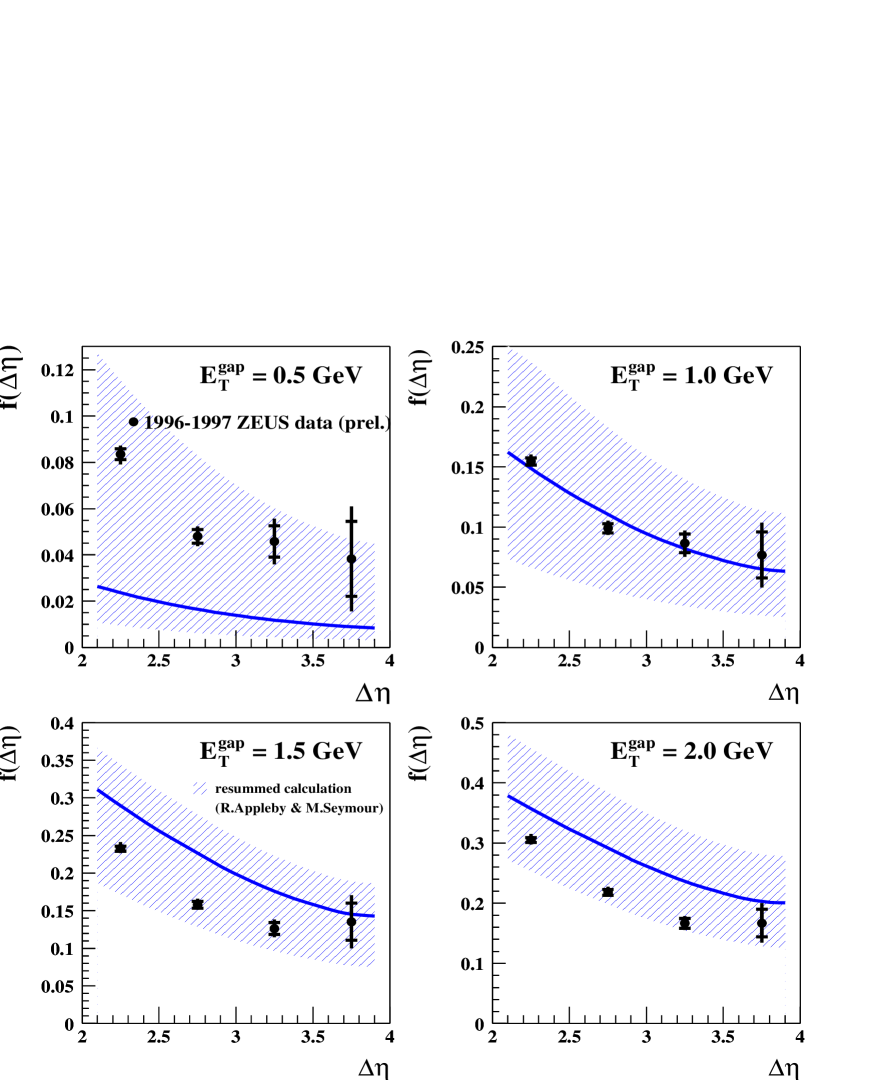
Figure I.1: The gap fractions for the ZEUS analysis with a kt defined final state, at varying $E_{T}^{\mathrm{gap}}(=Q_{\Omega})$. The (preliminary) ZEUS data is also shown. The solid line includes the effects of primary emission and the secondary emission suppression factor. The overall theoretical uncertainty, including the primary uncertainty and the secondary uncertainty, is shown by the shaded region.

Bibliography

- [1] R. K. Ellis, W. J. Stirling and B. R. Webber, Cambridge Monogr. Part. Phys. Nucl. Phys. Cosmol. 8 (1996) 1.
- [2] R. Brock et al. [CTEQ Collaboration], Rev. Mod. Phys. 67 (1995) 157.
- [3] M. E. Peskin and D. V. Schroeder, Reading, USA: Addison-Wesley (1995) 842 p.
- [4] G. Sterman, Cambridge, UK: Univ. Pr. (1993) 572 p.
- [5] J. A. Vermaseren, Comput. Phys. Commun. 83 (1994) 45.
- [6] J. C. Collins, D. E. Soper and G. Sterman, Nucl. Phys. B 308 (1988) 833.
- [7] N. Kidonakis, G. Oderda and G. Sterman, Nucl. Phys. B 525 (1998) 299
- [8] N. Kidonakis and J. F. Owens, Phys. Rev. D 63 (2001) 054019
- [9] C. F. Berger, SUNY PhD thesis, arXiv:hep-ph/0305076.
- [10] T. Regge, Nuov. Cim. 14 (1959) 951 Nuov. Cim. 18 (1960) 947.
- [11] J. R. Forshaw and D. A. Ross, Cambridge, UK: Univ. Pr. (1997) 248 p. (Cambridge lecture notes in physics. 9).
- [12] S. Donnachie, G. Dosch, O. Nachtmann and P. Landshoff, Cambridge, UK: Univ. Pr. (2002) 347 p.
- [13] P. D. Collins, Cambridge 1977, 445p.
- [14] G. F. P. Chew,S. C. Frautshi, Phys. Rev. Lett. 7 (1961) 394
- [15] A. Donnachie and P. V. Landshoff, Phys. Lett. B 296 (1992) 227
- [16] G. Corcella et al., JHEP 0101 (2001) 010
- [17] G. Corcella et al., “HERWIG 6.5 release note,” arXiv:hep-ph/0210213.
- [18] B. R. Webber, Ann. Rev. Nucl. Part. Sci. 36, 253 (1986).
- [19] B. R. Webber, Nucl. Phys. B 238 (1984) 492.
- [20] G. Marchesini and B. R. Webber, Nucl. Phys. B 310 (1988) 461.
- [21] J.C. Collins, Phys. Rev. D57 (1998) 3051; erratum-ibid D61 (1998) 019902.; J.C. Collins, hep-ph/0107252.
- [22] A. Berera, Phys. Rev. D62 (2000) 014015.
- [23] J.C. Collins, L. Frankfurt and M. Strikman, Phys. Rev. Lett. B307 (1993) 161.
- [24] A.D. Martin, M.G. Ryskin, V.A. Khoze, Phys. Rev. D. 56 (1997) 5867
- [25] G. Ingelman and P.E. Schlein, Phys. Lett. B142, 256 (1985).
- [26] T. Affolder et al, CDF Collaboration, Phys. Rev. Lett. 85 (2000) 4215.
- [27] B.E. Cox and J.R. Forshaw, Comput. Phys. Commun. 144 (2002) 104
- [28] C. Adloff et al, H1 Collaboration, Z. Phys. C76 (1997) 613.
- [29] L. Alvero, J.C. Collins and J.J. Whitmore, hep-ph/9806340.
- [30] J.D. Bjorken, Int. J. Mod. Phys. A7 (1992) 4189; Phys. Rev. D47 (1993) 101.
- [31] A.B. Kaidalov, V.A. Khoze, A.D. Martin and M.G. Ryskin, Eur. Phys. J. C 21 (2001) 521
- [32] E. Gotsman, E. Levin and U. Maor, Phys. Lett. B452 (1999) 387; Phys. Rev. D60 (1999) 094001.
- [33] M. Boonekamp, R. Peschanski and C. Royon, Phys. Rev. Lett. 87 (2001) 251806.
- [34] B. Cox, J. Forshaw and B. Heinemann, Phys. Lett. B 540 (2002) 263
- [35] R. B. Appleby and J. R. Forshaw, Phys. Lett. B 541 (2002) 108
- [36] G. Sterman and S. Weinberg, Phys. Rev. Lett. 39 (1977) 1436.
- [37] K. Goulianos [CDF Collaboration], arXiv:hep-ex/0109024.
- [38] G. C. Blazey and B. L. Flaugher, Ann. Rev. Nucl. Part. Sci. 49 (1999) 633
- [39] B. Heinemann, private communication.
- [40] A. Berera and J. C. Collins, Nuc. Phys. B474 (1996) 183; J. Pumplin, Phys. Rev. D52 (1995) 1477.
- [41] V.A. Khoze, A.D. Martin and M.G. Ryskin, Eur. Phys. J. C19 (2001) 477.
- [42] V.A. Khoze, A.D. Martin and M.G. Ryskin, Eur. Phys. J. C23 (2002) 311.
- [43] P. Thompson: ‘Jets and flows in diffraction at HERA’, talk presented at DIS 2002, April-May 2002, Acta Phys. Polon B 33, 3213 (2002).
- [44] J. R. Forshaw, Karlsruhe 2002, Hadron collider physic 199-211, arXiv:hep-ph/0212154.
- [45] B. E. Cox, J. R. Forshaw and L. Lonnblad, arXiv:hep-ph/0012310
- [46] J.F. Owens, Phys. Rev. D30 (1984) 943.
- [47] C. Adloff et al, H1 Collaboration, Eur. Phys. J. C6 (1999) 421.
- [48] H. Contopanagos, E. Laenen and G. Sterman, Nucl. Phys. B 484 (1997) 303
- [49] J. Botts and G. Sterman, Phys. Lett. B 224 (1989) 201 [Erratum-ibid. B 227 (1989) 501].
- [50] J. Botts and G. Sterman, Nucl. Phys. B 325 (1989) 62.
- [51] N. Kidonakis, Int. J. Mod. Phys. A 15 (2000) 1245
- [52] M. G. Sotiropoulos and G. Sterman, Nucl. Phys. B 419 (1994) 59
- [53] N. Kidonakis, G. Oderda and G. Sterman, Nucl. Phys. B 531 (1998) 365
- [54] N. Kidonakis and G. Sterman, Nucl. Phys. B 505 (1997) 321
- [55] C. F. Berger, T. Kucs and G. Sterman, Phys. Rev. D 65 (2002) 094031
- [56] E. L. Berger and H. Contopanagos, Phys. Rev. D 54 (1996) 3085
- [57] N. Kidonakis, Phys. Rev. D 64 (2001) 014009
- [58] G. Oderda, Phys. Rev. D 61 (2000) 014004
- [59] G. Oderda and G. Sterman, Phys. Rev. Lett. 81 (1998) 3591
- [60] M. Dasgupta and G. P. Salam, Phys. Lett. B 512 (2001) 323
- [61] M. Dasgupta and G. P. Salam, JHEP 0203 (2002) 017
- [62] C. Adloff et al. [H1 Collaboration], Eur. Phys. J. C 24 (2002) 517
- [63] ZEUS Collaboration, The XXXIth International Conference on High Energy Physics, Amsterdam, July 2002 Abstract number 852.
- [64] S. Catani, Yu. L. Dokshitzer, M. H. Seymour and B. R. Webber, Nucl. Phys. B 406 (1993) 187.
- [65] S. D. Ellis and D. E. Soper, Phys. Rev. D 48 (1993) 3160
- [66] J. M. Butterworth, J. P. Couchman, B. E. Cox and B. M. Waugh, Comput. Phys. Commun. 153 (2003) 85
- [67] S. Catani, M. L. Mangano, P. Nason and L. Trentadue, Nucl. Phys. B 478 (1996) 273
- [68] G. Sterman and M. E. Tejeda-Yeomans, Phys. Lett. B 552 (2003) 48
- [69] A. Banfi, G. Marchesini and G. Smye, JHEP 0208 (2002) 006
- [70] R. B. Appleby and M. H. Seymour, JHEP 0212 (2002) 063
- [71] R. B. Appleby and G. P. Salam, arXiv:hep-ph/0305232, presented at 38th Rencontres de Moriond on QCD and High-Energy Hadronic Interactions, Les Arcs, France, 22–29 March 2003.
- [72] G. C. Blazey et al., arXiv:hep-ex/0005012.
- [73] http://hepwww.rl.ac.uk/theory/seymour/ktclus/
- [74] Yu. L. Dokshitzer, G. Marchesini and G. Oriani, Nucl. Phys. B 387 (1992) 675.
- [75] C. F. Berger, T. Kucs and G. Sterman, Phys. Rev. D 68 (2003) 014012
- [76] Yu. L. Dokshitzer and G. Marchesini, JHEP 0303 (2003) 040.
- [77] G. Marchesini and B.R. Webber, Phys. Rev. D 38 (1988) 3419
- [78] Yu.L. Dokshitzer, V. Khoze and S. Troyan, in Physics in Collision VI, Proceedings of the International Conference, Chicago, Illinois, 1986, edited by M. Derrick (World Scientific, Singapore, 1987), p. 365.
- [79] J. D. Bjorken, Phys. Rev. D 47 (1993) 101.
- [80] M. Derrick et al. [ZEUS Collaboration], Phys. Lett. B 369 (1996) 55
- [81] R. B. Appleby and M. H. Seymour, JHEP 0309 (2003) 056
- [82] C. F. Weiszäcker, Z. Phys. 88 (1934) 612 ; E. J. Williams, Phys. Rev. 45 (1934) 729
- [83] M. Gluck, E. Reya and A. Vogt, Phys. Rev. D 46 (1992) 1973.
- [84] A. D. Martin, R. G. Roberts, W. J. Stirling and R. S. Thorne, Phys. Lett. B 443 (1998) 301
- [85] G. P. Korchemsky and G. Sterman, Nucl. Phys. B 555 (1999) 335
- [86] A. J. MacFarlane, A. Sudbery and P. H. Weiz, Commun. Math. Phys. 11 (1968) 77.