Scalar and Pseudoscalar Higgs Boson Plus One Jet Production
at the LHC and Tevatron

Abstract

The production of the Standard Model (SM) Higgs boson ($H$) plus one jet is compared with that of the lightest scalar Higgs boson ($h^{0}$) plus one jet and that of the pseudoscalar Higgs boson ($A^{0}$) plus one jet. The latter particles belong to the Minimal Supersymmetric Model (MSSM). We include both top and bottom quark loops to lowest order in QCD and investigate the limits of small quark mass and infinite quark mass. We give results for both the CERN Large Hadron Collider (LHC) and the Fermilab Tevatron.

I Introduction

The Higgs boson is the cornerstone of electroweak symmetry breaking in the Standard Model (SM). Particle physicists around the world have made the search for the Higgs boson the top priority in high energy experiments. However, there are several different candidate models in the Higgs sector. The Minimal Supersymmetric Standard Model (MSSM), which is a special case of the Two Higgs Doublet Model (2HDM), is of particular theoretical interest.

The Standard Model Higgs boson has been experimentally excluded by LEP searches for $e^{+}e^{-}\rightarrow ZH$ if its mass is lighter than approximately $114$ GeV​/c²lepfinal . In the MSSM, the particle spectrum includes five physical Higgs bosons; a light and a heavy neutral scalar ($h^{0},H^{0}$), two charged scalars ($H^{\pm}$), and a CP-odd pseudoscalar ($A^{0}$). The mass of the lightest scalar in the MSSM is excluded from being lighter than $91$ GeV​/c²neutral , while the mass of the pseudoscalar $M_{A^{0}}$ is experimentally excluded from being lighter than approximately $92$ GeV​/c². The ratio between the vacuum expectation values (VEVs) of the two neutral Higgs bosons of the MSSM is defined as $\tan\beta=v_{2}/v_{1}$. For $m_{\text{top}}=174.3$ GeV​/c², $0.5<\tan\beta<2.4$ has been excluded by the LEP Higgs searches. A different value of the top quark mass will lead to different exclusion bounds on $\tan\beta$.

The total cross-section for scalar Higgs production including massive quark loops has been calculated at next-to-leading order (NLO) in perturbative QCD spira1a ; graudenz ; spira1b . The corresponding calculation for Higgs production in the MSSM can be found in Ref. spira2a . In the Heavy Quark Effective Theory (HQET)nanopoulos ; hqet2 ; hqet1 , the top quark mass is assumed to be much heavier than the Higgs boson mass and all relevant energy scales. Assuming the HQET total inclusive cross-sections have been calculated at NLO for scalarsally and pseudoscalar productionschaffer ; spira2b and also at NNLO for scalarharkil1 ; harkil2 ; anast1 ; jack2 and for pseudoscalarjack2 ; harkil3 ; anast2 production, see alsocatani1 ; catani2 . The use of the HQET significantly simplifies the computation of higher order QCD effects and has been shown to accurately reproduce the exact NLO rate at the LHC for $pp\rightarrow H$spira1a ; spira1b for a Higgs mass less than $1$ TeV​/c² if the LO massive results are multiplied by the NLO K-factor obtained in the HQET.

In this paper we concentrate on the Higgs plus one jet ($gg\rightarrow g\Phi$, $qg\rightarrow q\Phi$, and $q\bar{q}\rightarrow g\Phi$) production processes since they are important for the experimental detection of the Higgs. Here $\Phi$ represents either the SM Higgs, $H$, or the MSSM scalars, $h^{0}$ and $H^{0}$, or the MSSM pseudoscalar $A^{0}$. The production of the SM Higgs plus one jet process has been calculated exactly at LO in ellis ; baur with the inclusion of heavy quark loops. The production rate in the MSSM for the lightest scalar plus one jet was recently calculated in LO including SUSY loop effects, which can be significant for light SUSY squarks and gluinoshollik . The NLO QCD corrections to the Higgs plus one jet process have only been computed in the HQET, since the full virtual corrections would require the evaluation of massive two-loop integrals for a $2\rightarrow 2$ reaction. The differential cross-section for the production of a scalar Higgs boson plus one jet in the HQET at NLO has been calculated previously by catani1 ; catani2 ; higgscross ; jack ; florian ; glosser and the integrated rate was shown to increase substantially from the lowest order rate. The pseudoscalar case has been presented in field2 and in kao .

We present the calculation of the Higgs plus one jet process where we include both top and bottom quark loops with the full quark mass dependence. This is done for the SM Higgs and for the lightest scalar and pseudoscalar Higgs bosons of the MSSM. The contributions of loops with bottom quarks can be important for large values of $\tan\beta$ in the MSSM. We also address the region of validity of the HQET predictions for these reactions.

In Section II, the limit of the partonic matrix elements in the HQET and in the small quark mass limit are explored. In Section III, the Higgs plus jet matrix elements are given and our computational techniques are described. Section IV summarizes our notation for the hadronic differential cross-sections. Section V contains numerical results for differential cross-sections at the Tevatron and LHC, as well as integrated results with cuts in transverse momemtum, $p_{t}$, and rapidity, $y$. Analytic results for the matrix elements are given in two Appendices.

$|\mathcal{M}|^{2}=|c_{t}^{\Phi}\mathcal{M}_{t}+c_{b}^{\Phi}\mathcal{M}_{b}|^{2}$

$\Phi$
$H$	$c_{t}^{H}=\;\;\;1$ $c_{b}^{H}=\;\;\;1$	$|\mathcal{M}|^{2}=|\mathcal{M}_{t}|^{2}+|\mathcal{M}_{b}|^{2}+2\textrm{Re}(\mathcal{M}_{t}\mathcal{M}_{b}^{\star})$
$h^{0}$	$\displaystyle c_{t}^{h^{0}}=\;\;\;\cos\alpha/\sin\beta$ $\displaystyle c_{b}^{h^{0}}=-\sin\alpha/\cos\beta$	$|\mathcal{M}|^{2}=\displaystyle\frac{\cos^{2}\!\alpha}{\sin^{2}\!\beta}|\mathcal{M}_{t}|^{2}+\frac{\sin^{2}\!\alpha}{\cos^{2}\!\beta}|\mathcal{M}_{b}|^{2}-2\frac{\sin\alpha\cos\alpha}{\sin\beta\cos\beta}\textrm{Re}(\mathcal{M}_{t}\mathcal{M}_{b}^{\star})$
$H^{0}$	$\displaystyle c_{t}^{H^{0}}=\;\;\;\sin\alpha/\sin\beta$ $\displaystyle c_{b}^{H^{0}}=\;\;\;\cos\alpha/\cos\beta$	$|\mathcal{M}|^{2}=\displaystyle\frac{\sin^{2}\!\alpha}{\sin^{2}\!\beta}|\mathcal{M}_{t}|^{2}+\frac{\cos^{2}\!\alpha}{\cos^{2}\!\beta}|\mathcal{M}_{b}|^{2}+2\frac{\sin\alpha\cos\alpha}{\sin\beta\cos\beta}\textrm{Re}(\mathcal{M}_{t}\mathcal{M}_{b}^{\star})$
$A^{0}$	$\displaystyle c_{t}^{A^{0}}=\;\;\;\cot\beta$ $\displaystyle c_{b}^{A^{0}}=\;\;\;\tan\beta$	$|\mathcal{M}|^{2}=\displaystyle\frac{1}{\tan^{2}\!\beta}|\mathcal{M}_{t}|^{2}+\tan^{2}\!\beta|\mathcal{M}_{b}|^{2}+2\textrm{Re}(\mathcal{M}_{t}\mathcal{M}_{b}^{\star})$

Table 1: Higgs-fermion couplings in the MSSM and the dependence of the matrix element-squared on the couplings. $\mathcal{M}_{t}$ and $\mathcal{M}_{b}$ represent contributions from top- and bottom- quark loops, respectively. The $\alpha$ parameter is the angle that diagonalizes the CP-even Higgs squared-mass matrix.

II Partonic Processes - Heavy Quark Effective Theory

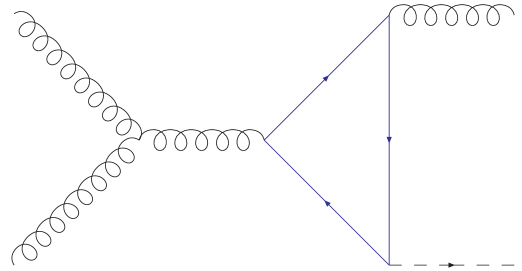
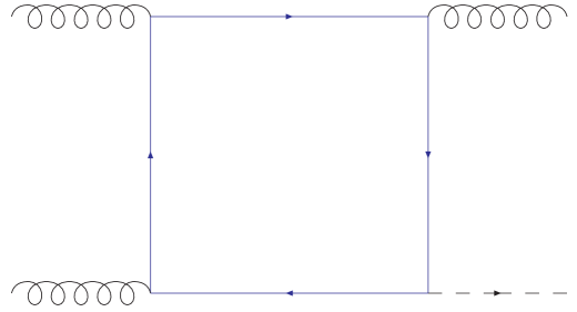
(a)	(b)
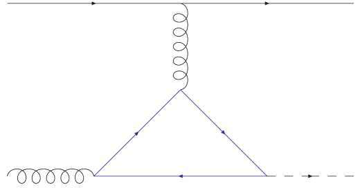
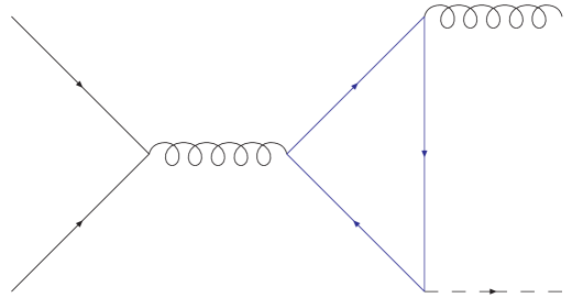
(c)	(d)

Figure 1: Sample Higgs plus one jet diagrams. Figures 1a,b are the $gg$ diagrams, 1c is the $qg$ channel, and 1d is the $q\bar{q}$ channel. All quarks contribute to the loops. The crossed and charge conjugate diagrams are not shown. There are a total of $12$ $gg$ diagrams and $2$ for each of the $qg$ and $q\bar{q}$ sub-processes.

In the limit where the top quark mass is much heavier than all the energy scales in the problem, only the top quark coupling to gluons is numerically significant and this limit provides a good approximation to Standard Model Higgs production matrix elements. The HQET limit for scalar Higgs production has been extensively studied in the literature. This limit is especially useful for deriving higher order QCD corrections since the massive top quark loops that couple the Higgs boson to gluons reduce to effective vertices. The Feynman rules can be derived from an effective Lagrangian densityspira1a ; spira1b ; hqet1 ; hqet2 ; sally ; harkil1 ,

$$\mathcal{L}_{\text{eff}}^{H}=-g_{H}\frac{H}{4v}{\mathcal{C}}_{H}(\alpha_{s})\mathcal{O}_{H},\quad\mathcal{O}_{H}=G^{a}_{\mu\nu}G^{a,\mu\nu},$$ (1)

where $g_{H}=1$ in the Standard Model and $v=246$ GeV. ${\mathcal{O}}_{H}$ generates vertices which couple the Higgs boson to two, three, and four gluons. In the large $m_{\text{top}}$ limit, the coefficient ${\mathcal{C}}_{H}$ can be evaluated as a power series in $\alpha_{s}$spira1a ; spira1b ; hqet2 ; hqet1 ; hqet_h1 ; hqet_h2 ; hqet_h3

$$\mathcal{C}_{H}(\alpha_{s}^{(5)}(\mu_{r}^{2}))=-\frac{\alpha_{s}^{(5)}(\mu_{r}^{2})}{3\pi}\biggl{[}1+\frac{11\alpha_{s}^{(5)}(\mu_{r}^{2})}{4\pi}+\cdots\biggr{]},$$ (2)

where $\alpha_{s}^{(5)}(\mu_{r}^{2})$ is evaluated at the scale $\mu_{r}$ in a $5$ flavor scheme.

For comparison, we consider a pseudoscalar Higgs boson with a coupling to fermions given by,

$$\mathcal{L}_{\text{eff}}^{A^{0}}=-ig_{A}\frac{{A^{0}}}{v}m_{i}{\overline{\psi}}_{i}\gamma_{5}\psi_{i}.$$ (3)

In the large $m_{\text{top}}$ limit, the interactions of the pseudoscalar with gluons can be found from the effective Lagrangian harkil2 ; russel2 ; footnote ; hqet_a1

$$\mathcal{L}_{\text{eff}}^{A^{0}}=-g_{A}\frac{{A^{0}}}{v}\bigl{(}C_{A_{1}}(\alpha_{s})\mathcal{O}_{1}+C_{A_{2}}(\alpha_{s})\mathcal{O}_{2}\bigr{)},\quad\mathcal{O}_{1}=\epsilon_{\mu\nu\lambda\sigma}G^{\mu\nu}_{a}G^{\lambda\sigma}_{a},\quad\mathcal{O}_{2}=\partial^{\mu}\sum^{n_{f}}_{i=0}\bar{q}_{i}\gamma_{\mu}\gamma_{5}q_{i},$$ (4)

where $G^{\mu\nu}_{a}$ is the gluon field strength tensor. The process independent coefficient functions are

$$C_{A_{1}}=-\frac{\alpha_{s}(\mu_{r}^{2})}{16\pi},\qquad C_{A_{2}}=\;{\cal O}(\alpha_{s}^{2}).$$ (5)

We consider $g_{A}=1$ and the examine the differences between differential cross-sections for the production of a SM scalar Higgs boson and a pseudoscalar Higgs boson with the couplings of Eq. 3, when the bosons are produced in association with a jet.

It is also of interest to compare the production rates for a Higgs boson plus a jet in the MSSM. The effective Lagrangians in this case are found by making the replacements in Eqs. 1 and 4,

$$g_{H}\rightarrow c_{t}^{h^{0}}$$

$$g_{A}\rightarrow c_{t}^{A^{0}},$$ (6)

where $c_{t}^{h^{0}}$ and $c_{t}^{A^{0}}$ are given in Table I. (We neglect contributions from SUSY particles such as the bottom squarks and gluinos, and therefore assume that the SUSY particle masses are much larger than $m_{\text{top}}$ and $m_{\Phi}$. These genuine SUSY contributions can be important for light squark and gluino masseshollik .) When the bottom quark becomes important, the HQET breaks down as a reliable calculational tool. This occurs in the MSSM when $\tan\beta$ becomes large and the bottom quark couplings are enhanced.

Figure 2: The squared matrix elements, $|\mathcal{M}|^{2}$, evaluated at $\hat{s}=4m_{\Phi}^{2}$ and $\hat{u}=\hat{t}$ for the three different channels, ($gg$, $qg$, $q\bar{q}$), normalized to the squared matrix elements in the HQET for scalar and pseudoscalar (with $g_{A}=1$) Higgs plus jet production. We include only the top quark loops. The solid line is the scalar, whereas the dashed line is the pseudoscalar.

III Partonic Processes - Full Theory

There are three channels associated with Higgs plus one jet production: gluon fusion, quark-gluon scattering, and quark-antiquark annihilation. Representative Feynman diagrams are shown in Fig. 1. At the LHC where $\sqrt{S}=14$ TeV the gluon fusion and quark-gluon channels are the most important, with the quark-antiquark channel adding a negligible amount to the process. However all three channels are important at the Tevatron where $\sqrt{S}=1.96$ TeV.

The calculation of the matrix elements was carried out in both $n=4-2\epsilon$ dimensions and $4$-dimensions. The $\gamma_{5}$ in the pseudoscalar calculation was treated using the Akyeampong-Delbourgo prescriptionad1 ; ad2 ; ad3 for the $\gamma_{5}$-matrix. In this scheme the $\gamma_{5}$ is exchanged for a Levi-Civita tensor contracted with four $\gamma$-matrices. After the trace, the tensor loop integrals were reduced to scalar integrals using the usual Passarino-Veltmanloops reduction techniques.

III.1 Gluon fusion ($gg\rightarrow g\Phi$)

The gluon fusion channel is the most important channel at the LHC. The momentum distribution in this process is assigned with all momentum incoming,

$$g(p_{1}^{\mu_{1},a_{1}})+g(p_{2}^{\mu_{2},a_{2}})\rightarrow g(-p_{3}^{\mu_{3},a_{3}})+\Phi(-p_{5}),$$ (7)

where $\mu_{i}$ are Lorentz indices and $a_{i}$ are color indices. The Mandelstam variables used in the partonic system are

$$\hat{s}=(p_{1}+p_{2})^{2},\quad\hat{t}=(p_{1}+p_{5})^{2},\quad\hat{u}=(p_{2}+p_{5})^{2},\quad Q^{2}=m^{2}_{\Phi}.$$ (8)

The matrix elements, including the gluon polarization vectors, can be written

$$\mathcal{M}^{gg}=\epsilon^{\mu_{1}}(p_{1})\epsilon^{\mu_{2}}(p_{2})\epsilon^{\mu_{3}}(p_{3})\mathcal{M}^{gg}_{\mu_{1}\mu_{2}\mu_{3}}.$$ (9)

The Ward-Takahashi identities let us check the gauge invariance of the sub-process. In the gluon fusion case, these can be written as

$$p_{1}^{\mu_{1}}\epsilon^{\mu_{2}}(p_{2})\epsilon^{\mu_{3}}(p_{3})\mathcal{M}^{gg}_{\mu_{1}\mu_{2}\mu_{3}}=\epsilon^{\mu_{1}}(p_{1})p_{2}^{\mu_{2}}\epsilon^{\mu_{3}}(p_{3})\mathcal{M}^{gg}_{\mu_{1}\mu_{2}\mu_{3}}=\epsilon^{\mu_{1}}(p_{1})\epsilon^{\mu_{2}}(p_{2})p_{3}^{\mu_{3}}\mathcal{M}^{gg}_{\mu_{1}\mu_{2}\mu_{3}}=0,$$ (10)

giving us a strong check on the algebraic results. Analytic results for the matrix element squared for $gg\rightarrow gA^{0}$ are given in Appendix A, see also Appendix C in spira1b , while those for $gg\rightarrow gH$ can be found in Refs. baur ; ellis .

III.2 Quark-antiquark annihilation ($q\bar{q}\rightarrow g\Phi$)

For this sub-process, the momentum, color, and Lorentz structure was assigned as follows

$$q(p_{1})+\bar{q}(p_{2})\rightarrow g(-p_{3}^{\mu_{3},a_{3}})+\Phi(-p_{5}).$$ (11)

The matrix elements satisfy

$$\mathcal{M}^{q\bar{q}}=\epsilon^{\mu_{3}}(p_{3})\mathcal{M}^{q\bar{q}}_{\mu_{3}},\qquad p_{3}^{\mu_{3}}\mathcal{M}^{q\bar{q}}_{\mu_{3}}=0.$$ (12)

Analytic results for $q{\overline{q}}\rightarrow gA^{0}$ are given in Appendix B, see also Appendix C in spira1b , while those for $q{\overline{q}}\rightarrow gH$ can be found in Refs. baur ; ellis . The results for quark-gluon scattering can be found by crossing.

III.3 HQET Matrix Elements

The $4$-dimensional color-spin averaged matrix elements for Higgs boson plus one jet production in the $m_{\text{top}}\rightarrow\infty$ limit are presented here for completeness. These matrix elements obey the same crossing relations as the full matrix elements,

$$|\mathcal{M}(\hat{s},\hat{t},\hat{u})|^{2}_{qg\rightarrow q\Phi}=-|\mathcal{M}(\hat{u},\hat{t},\hat{s})|^{2}_{q\bar{q}\rightarrow g\Phi}.$$ (13)

The matrix elements in the large $m_{\text{top}}$ HQET limit can be writtenspira1b ; baur ; ellis ; kao ,

$$\overline{\sum}|\mathcal{M}|^{2}_{gg\rightarrow g\Phi} =A_{\Phi}\frac{N_{c}}{4(N_{c}^{2}-1)}\;\frac{\hat{s}^{4}+\hat{t}^{4}+\hat{u}^{4}+Q^{8}}{\hat{s}\hat{t}\hat{u}}$$ (14)

$$\overline{\sum}|\mathcal{M}|^{2}_{qg\rightarrow q\Phi} =-A_{\Phi}\frac{1}{8N_{c}}\;\frac{\hat{s}^{2}+\hat{t}^{2}}{\hat{u}}$$ (15)

$$\overline{\sum}|\mathcal{M}|^{2}_{q\bar{q}\rightarrow g\Phi} =A_{\Phi}\frac{(N_{c}^{2}-1)}{8N_{c}^{2}}\;\frac{\hat{u}^{2}+\hat{t}^{2}}{\hat{s}},$$ (16)

where,

$$A_{H}= \biggl{(}\frac{\alpha_{s}}{3\pi v}\biggr{)}^{2}(4\pi\alpha_{s})g_{H}^{2}$$

$$A_{A}= \biggl{(}\frac{\alpha_{s}}{2\pi v}\biggr{)}^{2}(4\pi\alpha_{s})g_{A}^{2}$$ (17)

and $g_{H}=1$ for the SM and $g_{\Phi}$ is given in Eq. 6 for the MSSM. The bar implies a sum and average over colors and spins. The exact matrix elements squared as compared with the HQET matrix elements are shown in Fig. 2 for both the SM scalar, which are in excellent agreement with the plots in baur , and for a pseudoscalar with $g_{A}=1$. In this plot, the mass of the Higgs was set to $m_{\Phi}=100$ GeV​/c² and the mass of the top quark was varied. In these plots, two thresholds can be observed. Each threshold occurs when an imaginary part of the matrix elements turns on or off. If we examine Eq. 53 for $q\bar{q}\rightarrow gA^{0}$ we clearly see that the imaginary part contains the difference of two step functions

$$\theta(\hat{s}-4m_{\text{top}}^{2})-\theta(M^{2}_{A^{0}}-4m_{\text{top}}^{2}),$$ (18)

so the first threshold occurs at $2m_{\text{top}}=M_{A^{0}}$ and the second at $2m_{\text{top}}=\sqrt{\hat{s}}$. Since we choose $\hat{s}=4M_{A^{0}}^{2}$ for the plot this implies that these thresholds occur at $m_{\text{top}}/m_{\Phi}=0.5$ and $1$ respectively. The imaginary part is finite between these cusps. Similar phenomena occur in the other reactions. However when the squared matrix elements contain several terms the onset of the imaginary parts is not always visible. The reactions $qg\rightarrow q\Phi$ do not have $\hat{s}$ channels so they only have cusps at $m_{\text{top}}/m_{\Phi}=0.5$. Finally the $gg\rightarrow g\Phi$ channels show both cusps. Note that the reason the cusps do not appear exactly at $0.5$ and $1$ is due to our choice of points in $m_{\text{top}}/m_{\Phi}$.

These ratios show that when the heavy quark becomes heavier than $m_{\text{top}}\sim\frac{1}{2}m_{\Phi}$ the HQET is a reasonable approximation to the matrix elements with a top loop only. In the MSSM, however, the usefulness of the HQET is limited to small values of $\tan\beta$ where the bottom quark contribution can be neglected.

III.4 Small Quark Mass Limit

When the quark mass in the loop is much smaller than the Higgs mass and the energy scale, the small quark mass limit $m_{f}\rightarrow 0$ is relevant. This is the case for the bottom quark contribution in the large $\tan\beta$ limit of the MSSM. The matrix elements in this limit behave as

$$|\mathcal{M}|^{2}\sim m_{f}^{4}\log^{4}(m_{f}^{2}/\mu^{2}),$$ (19)

where $\mu>\!\!>m_{f}$. Exact expressions in the small quark mass limit are given in Appendix B.

IV Observables

Generically, we can write a $2\rightarrow 2$ differential observable as

$$\hat{s}^{2}\frac{d^{2}\!\hat{\sigma}}{d\hat{t}\;d\hat{u}}=\frac{1}{16\pi}\;\overline{\sum}|\mathcal{M}|^{2},$$ (20)

where the bar implies a sum and average over colors and spins. To relate the hadronic differential distributions to the partonic differential distributions we need to perform a convolution with the parton distribution functions.

The hadronic process can be written as

$$H_{1}(P_{1})+H_{2}(P_{2})\rightarrow j(-p_{3})+\Phi(-p_{5})$$ (21)

where the $j$ represents the gluon or the quark jet in the sub-process of interest. In the hadronic system, we can write

$$S=(P_{1}+P_{2})^{2},\quad T=(P_{1}+p_{5})^{2},\quad U=(P_{2}+p_{5})^{2}.$$ (22)

This translates into the partonic system (with momentum fractions $x_{1}$ and $x_{2}$) as

$$p_{1}=x_{1}P_{1},\quad p_{2}=x_{2}P_{2},$$ (23)

$$\hat{s}=x_{1}x_{2}S,\quad\hat{t}=x_{1}(T-Q^{2})+Q^{2},\quad\hat{u}=x_{2}(U-Q^{2})+Q^{2}$$ (24)

$$x_{1,\text{min}}=\frac{-U}{S+T-Q^{2}},\quad x_{2,\text{min}}=\frac{-x_{1}(T-Q^{2})-Q^{2}}{x_{1}S+U-Q^{2}},$$ (25)

where $Q^{2}=m_{\Phi}^{2}$. The hadronic variables can be written in terms of the transverse momentum and rapidity

$$T =Q^{2}-\sqrt{S}\sqrt{p_{t}^{2}+Q^{2}}\cosh y+\sqrt{S}\sqrt{p_{t}^{2}+Q^{2}}\sinh y$$ (26)

$$U =Q^{2}-\sqrt{S}\sqrt{p_{t}^{2}+Q^{2}}\cosh y-\sqrt{S}\sqrt{p_{t}^{2}+Q^{2}}\sinh y.$$ (27)

The hadronic differential cross-section is,

$$S^{2}\frac{d^{2}\!\sigma^{H_{1}H_{2}}}{dT\;dU}=\sum_{ab}\int^{1}_{x_{1,\text{min}}}\frac{dx_{1}}{x_{1}}\int^{1}_{x_{2,\text{min}}}\frac{dx_{2}}{x_{2}}\;f^{H_{1}}_{a}(x_{1},\mu_{f}^{2})f^{H_{2}}_{b}(x_{2},\mu_{f}^{2})\;\hat{s}^{2}\frac{d^{2}\!\hat{\sigma}_{ab}}{d\hat{t}\;d\hat{u}}.$$ (28)

Upon further integration we obtain the single differential $p_{t}$ and rapidity distributions with the kinematic limits,

$$p_{t,\text{max}}=\frac{1}{2}\frac{S-Q^{2}}{\sqrt{S}},\quad y_{\text{max}}=\frac{1}{2}\ln\biggl{(}\frac{1+S_{Q}}{1-S_{Q}}\biggr{)},$$ (29)

$$\text{where}\quad S_{Q}=\sqrt{1-\frac{4S(p_{t}^{2}+Q^{2})}{(S+Q^{2})^{2}}}.$$ (30)

V Numerical Results

We present our calculations for the CERN LHC with $\sqrt{S}=14$ TeV and the Fermilab Tevatron with $\sqrt{S}=1.96$ TeV. We use the CTEQ6.1L parton distribution functionscteq with $\Lambda_{5}^{\text{LO}}=165.2$ MeV and a one loop running coupling constant with $\alpha_{s}(M_{Z})=0.1298$. For the differential distributions, the full kinematic rapidity and $p_{t}$ are used and the factorization and renormalization scales are set equal to,

$$\mu_{r}=\mu_{f}=\sqrt{Q^{2}+p_{t}^{2}}.$$ (31)

We use pole masses with $m_{\text{top}}=174.3$ GeV​/c² and $m_{\text{bot}}=4.5$ GeV​/c². For the integrated cross-section we require the $p_{t}$ of the Higgs and the jet to satisfy $p_{t,\text{min}}>30$ GeV​/c in the rapidity region $|y|<2.5$ and replace $p_{t}$ by $p_{t,\text{min}}$ in Eq. 31 for the renormalization and factorization scales.

V.1 Standard Model

Figure 3: Transverse momentum distributions for the SM Higgs boson plus one jet production at the LHC with $M_{H}=120$ GeV​/c² for the different channels. The curves labeled ‘Top’ (‘Bot’) include ${\it only}$ the top (bottom) quark loops.

The transverse momentum distributions of the SM Higgs boson for all the separate channels are shown in Fig. 3 for the LHC. For a SM Higgs boson with $M_{H}=120$ GeV​/c², the cross-section for Higgs plus one jet is approximately $12.3$ pb when both the top and bottom quarks are included in the calculation. Although the bottom quark contribution alone is only $0.05$ pb, the top-bottom interference lowers the cross-section by approximately $8.25$% from $13.4$ pb when only the top quark is included, see sally2 . This lowering of the cross-section may be visible at the LHC. As shown in Fig. 4, the full theory and the HQET agree very well at small to moderate $p_{t}$ for both the scalarellis ; glosser and the pseudoscalar differential distributions.

Figure 4: Transverse momentum distributions for the SM Higgs ($H$) plus one jet and for a pseudoscalar ($A^{0}$) plus one jet in the full theory with only the top-quark loops included and in the HQET at the LHC for $M_{\Phi}=120$ GeV​/c². We assume $g_{A}=1$.

Figure 5: The transverse momentum distributions for the MSSM pseudoscalar Higgs boson for $\tan\beta=30,40,50$ and $M_{A^{0}}=120$ GeV​/c² at the Tevatron including the top and bottom quark loops. The top, middle, and bottom lines in the top graph are the curves for $\tan\beta=50,40,30$ respectively. Below is the fraction of the process that comes from each of the different channels. The curves at $p_{t}=250$ GeV​/c from top to bottom are the $qg$, $gg$, and $q\bar{q}$ channels respectively.

V.2 Minimal Supersymmetric Standard Model

The MSSM is a special case of the 2HDM. In the MSSM, the up- and down-type quarks become massive from different Higgs doublets and the ratio of the two VEVs is parameterized by $\tan\beta=v_{2}/v_{1}$. As shown in Table 1, up- and down-type quarks couple differently to the Higgs bosons of the MSSM. The $\alpha$ parameter is the angle that is introduced to diagonalize the mass eigenstates of the CP-even Higgs squared-mass matrix to obtain the physical states. The program HDECAYhdecay was used to determine the mass of the lightest scalar and the $\alpha$ mixing parameter once the values of $M_{A^{0}}$ and $\tan\beta$ were chosen. The SUSY Higgs mixing parameter was set to $\mu=300$ GeV​/c², the gluino mass to $\mu_{2}=200$ GeV​/c², all the SUSY breaking masses to $1$ TeV​/c², and the soft breaking term to $1.5$ TeV​/c².

At the Tevatron, there is a very small signal for the SM Higgs boson. The cross-section for a SM Higgs boson plus one jet with $M_{H}=120$ GeV​/c² at lowest order in QCD is approximately $0.1$ pb. For $\tan\beta\sim 30$ the cross-section for a $120$ GeV​/c² pseudoscalar Higgs in the MSSM is about twice as large as for a $120$ GeV​/c² SM Higgs at the Tevatron and continues to grow with $\tan\beta$. The differential cross-section for pseudoscalar plus jet production at the Tevatron is shown in Fig. 5. At the Tevatron, the large $\tan\beta$ region is completely dominated by bottom quark loops where the HQET is of little use.

For the LHC, the entire $\tan\beta$ region is experimentally accessible. In the small $\tan\beta$ region, the cross-section is well approximated by the HQET limit and the bottom quark contribution can be neglected. However, there are regions where both the top and bottom quark loops are important. The results are summarized in Figs. 6 and  7. These plots use the full theory matrix elements. For pseudoscalar plus jet production, including only the top quark loop underestimates the total cross-section by $9.5$% at $\tan\beta=4$ and the discrepancy becomes larger as $\tan\beta$ grows. Including only the bottom quark underestimates the total cross-section by $5.6$% at $\tan\beta=8$ and becomes a better approximation as $\tan\beta$ increases. The total cross-section for the MSSM lightest scalar plus jet production receives an important contribution from the interference between the top- and bottom-quark loops over a large range of $\tan\beta$.

Figure 6: Cross-section for the production of the MSSM pseudoscalar Higgs boson plus one jet for different values of $\tan\beta$ at the LHC for $M_{A^{0}}=120$ GeV​/c² integrated for $p_{t}>30$ GeV​/c using the full theory matrix elements. The top and bottom labels show what the contribution of the top and bottom quark would be alone. In the region $4<\tan\beta<8$ the total cross-section is not represented well by either the top or bottom matrix elements alone. In the experimentally accessible region, the total cross-section at the Tevatron is dominated by the bottom loop so only the bottom contribution is shown for $\tan\beta>30$.

Figure 7: Cross-section for the production of the MSSM lightest scalar Higgs boson plus one jet for different values of $\tan\beta$ integrated for $p_{t}>30$ GeV​/c using the full theory matrix elements. The top and bottom labels show what the contributions of the top and bottom quark would be alone. In the experimentally accessible region, the total cross-section at the Tevatron is dominated by the bottom loop, so only the bottom contribution is shown for $\tan\beta>30$. Below is the corresponding mass of the lightest scalar for $M_{A^{0}}=120$ GeV​/c².

VI Conclusions

We calculated the differential distributions and cross-sections for the SM Higgs, $H$, the MSSM scalar Higgs boson, $h^{0}$, and pseudoscalar boson, $A^{0}$, plus one jet production at the Tevatron and LHC. We included both the top and bottom quark loops and investigated the validity of the Heavy Quark Effective Theory (HQET) limit and the light quark mass limit. For large $\tan\beta$, the HQET fails and the complete result with all mass dependences is needed.

The NLO QCD corrections for Higgs plus jetjack ; florian ; glosser and pseudoscalar plus jetfield2 production have been previously found in the large $m_{\text{top}}$ limit. Our results make it clear that these can only be applied to the MSSM in certain regions. At large $\tan\beta$, using the bottom-quark only is a very good approximation in the MSSM. At small $\tan\beta$ the MSSM pseudoscalar is top-quark loop dominated, whereas the lightest scalar in the MSSM still receives important contributions from both the top- and bottom-quarks over a much broader range of $\tan\beta$. This can be seen as the effective suppression of the $c_{t}^{h^{0}}$ coupling and enhancement of the $c_{b}^{h^{0}}$ coupling at small $\tan\beta$ where the interference between the two terms is still playing an important role.

Appendix A Complete Pseudoscalar Matrix Elements

For the $q\bar{q}\rightarrow gA^{0}$ sub-process, the (spin and color averaged) matrix elements squared are particularly simple because the presence of a $\gamma_{5}$ makes the traces much smaller than in the scalar case. They can be written in terms of the integrals presented inbaur ,

$$\overline{\sum}|\mathcal{M}|^{2}_{q{\overline{q}}\rightarrow gA^{0}}=\frac{16m_{f}^{4}}{\hat{s}}\biggl{(}\frac{(4\pi\alpha_{s}(\mu_{r}^{2}))^{3}}{4N_{c}^{2}v^{2}}\biggr{)}\;|C_{1}(\hat{s})|^{2}\;[\hat{s}^{2}-2\hat{t}_{1}\hat{u}_{1}+Q^{4}],$$ (32)

where the new variables are defined

$$\hat{s}_{1}=\hat{s}-Q^{2},\quad\hat{t}_{1}=\hat{t}-Q^{2},\quad\hat{u}_{1}=\hat{u}-Q^{2}.$$ (33)

It is easy to see that $\hat{s}_{1}=-(\hat{t}+\hat{u})$ and so on.

In these expressions we use the notation of baur . The $C_{1}$ loop integral that appears in the calculation is the usual triangle integral with two massive legs. For $p_{1}^{2}=0$, $p_{2}^{2}=Q^{2}=m_{\Phi}^{2}$, $p_{12}=p_{1}+p_{2}$ and $p_{12}^{2}=\hat{s}$, the triangle integral is defined as

$$C_{1}(\hat{s}) =C_{1}(p_{1},p_{2})$$ (34)

$$=\frac{1}{i\pi^{2}}\int\frac{d^{4}\!q}{[q^{2}-m_{f}^{2}][(q+p_{1})^{2}-m_{f}^{2}][(q+p_{12})^{2}-m_{f}^{2}]}.$$ (35)

The box integrals with $p_{1}^{2}=p_{2}^{2}=p_{3}^{3}=0$, and $p_{123}^{2}=(p_{1}+p_{2}+p_{3})^{2}=Q^{2}$ are defined as

$$D(\hat{s},\hat{t}) =D(p_{1},p_{2},p_{3})$$ (36)

$$=\frac{1}{i\pi^{2}}\int\frac{d^{4}\!q}{[q^{2}-m_{f}^{2}][(q+p_{1})^{2}-m_{f}^{2}][(q+p_{12})^{2}-m_{f}^{2}][(q+p_{123})^{2}-m_{f}^{2}]}.$$ (37)

It is easy to see that the box integrals satisfy the relation $D(\hat{x},\hat{y})=D(\hat{y},\hat{x})$. The computer package FFff was used to evaluate the scalar integrals.

For the $gg\rightarrow gA^{0}$ sub-process, the (spin and color averaged) matrix element squared can be written in the symmetric form,

$$\overline{\sum}|\mathcal{M}|^{2}_{gg\rightarrow gA^{0}}=\sum_{f}\frac{m_{f}^{4}(4\pi\alpha_{s}(\mu_{r}^{2}))^{3}}{v^{2}(N_{c}^{2}-1)^{2}}\biggl{\{} F(\hat{s},\hat{t},\hat{u})+F(\hat{s},\hat{u},\hat{t})+F(\hat{u},\hat{s},\hat{t})+F(\hat{u},\hat{t},\hat{s})+F(\hat{t},\hat{u},\hat{s})+F(\hat{t},\hat{s},\hat{u})\biggr{\}}$$ (38)

where

$$F(\hat{s},\hat{t},\hat{u})= -2\;\text{Re}\biggl{(}C_{1}(\hat{u})D^{*}(\hat{u},\hat{s})\biggr{)}\biggl{[}\hat{s}_{1}\biggl{(}\frac{\hat{s}Q^{2}}{\hat{t}}+\hat{u}\biggr{)}-\hat{s}\hat{t}-\frac{\hat{s}^{3}}{\hat{t}}\biggr{]}-\frac{1}{2}\;\text{Re}\biggl{(}D(\hat{s},\hat{t})D^{*}(\hat{u},\hat{s})\biggr{)}\biggl{[}\hat{t}_{1}(\hat{s}^{2}+\hat{s}\hat{t})\biggr{]}$$

$$+2\;\text{Re}\biggl{(}C_{1}(\hat{t})C_{1}^{*}(\hat{u})\biggr{)}\biggl{[}\frac{\hat{t}^{2}-\hat{t}_{1}Q^{2}}{\hat{s}}+Q^{2}\biggl{(}\frac{Q^{4}+2\hat{s}\hat{s}_{1}}{\hat{u}\hat{t}}\biggr{)}+\hat{t}-3Q^{2}+4\hat{s}\biggr{]}$$

$$-|C_{1}(\hat{u})|^{2}\biggl{[}\frac{Q^{6}\hat{u}_{1}}{\hat{s}\hat{t}\hat{u}}+\frac{\hat{s}^{2}+Q^{4}}{\hat{t}}+\frac{\hat{t}^{2}+Q^{4}}{\hat{s}}-\frac{4\hat{s}\hat{t}-3Q^{4}}{\hat{u}}-3Q^{2}\biggr{]}$$

$$+\text{Re}\biggl{(}C_{1}(\hat{u})D^{*}(\hat{s},\hat{t})\biggr{)}\biggl{[}\hat{s}\hat{t}-\hat{s}_{1}\hat{t}_{1}+Q^{2}\biggl{(}\frac{\hat{s}_{1}^{2}+\hat{s}^{2}}{\hat{u}}\biggr{)}\biggr{]}$$

$$-\frac{1}{4}|D(\hat{s},\hat{t})|^{2}\biggl{(}2(\hat{s}^{3}+\hat{t}^{3})-\frac{\hat{s}^{2}\hat{t}^{2}}{\hat{u}}+\frac{\hat{s}\hat{t}}{\hat{u}^{2}}\biggl{[}(\hat{s}+\hat{t})^{3}-2\hat{s}\hat{t}\hat{u}\biggr{]}\biggr{)}.$$ (39)

Appendix B Analytic Limits of Matrix Elements

The partonic cross-section for $q\overline{q}\rightarrow g\Phi$ is

$$\frac{d\hat{\sigma}}{d\hat{t}}=\frac{1}{16\pi\hat{s}^{2}}\frac{1}{36}|\mathcal{M}|^{2}_{q{\overline{q}}\rightarrow g\Phi},$$ (40)

where the spin and color average is explicitly given,

$$|\overline{\mathcal{M}}|^{2}_{q\overline{q}\rightarrow g\Phi}\equiv\frac{1}{36}|\mathcal{M}|^{2}_{q{\overline{q}}\rightarrow g\Phi}.$$ (41)

For a scalar Higgs,

$$|\mathcal{M}|^{2}_{q{\overline{q}}\rightarrow gH}=\frac{16\alpha_{s}^{3}}{\pi v^{2}}\frac{\hat{t}^{2}+\hat{u}^{2}}{\hat{s}}|A_{q\overline{q}}^{H}|^{2},$$ (42)

and

$$A_{q\overline{q}}^{H}=\sum_{j}\biggl{\{}\frac{m_{j}^{2}}{\hat{s}-M_{H}^{2}} \biggl{[}2-\frac{2\hat{s}}{\hat{s}-M_{H}^{2}}\biggl{(}I_{1}(\hat{s}/m_{j}^{2})-I_{1}(M_{H}^{2}/m_{j}^{2})\biggr{)}$$

$$+\biggl{(}1+\frac{4m_{j}^{2}}{\hat{s}-M_{H}^{2}}\biggr{)}\biggr{(}I_{2}(\hat{s}/m_{j}^{2})-I_{2}(M_{H}^{2}/m_{j}^{2})\biggr{)}\biggr{]}\biggr{\}},$$ (43)

where $m_{j}$ is the fermion mass in the loop. The integrals are defined by:

$$I_{1}(a)=\int_{0}^{1}dx\log\biggl{(}1-ax(1-x)\biggr{)},\quad I_{2}(a)=\int_{0}^{1}\frac{dx}{x}\log\biggl{(}1-ax(1-x)\biggr{)}.$$ (44)

In the large fermion mass limit, $m_{j}\rightarrow\infty$,baur ; ellis

$$A_{q\overline{q}}^{H}\rightarrow-\frac{1}{3}\biggl{(}1+\frac{1}{120}\frac{11\hat{s}+7M_{H}^{2}}{m_{j}^{2}}+\ldots\biggr{)}.$$ (45)

In the small fermion mass limit, $m_{j}\rightarrow 0$,baur

$$A_{q\overline{q}}^{H} \rightarrow A_{q\overline{q}}^{Hr}+iA_{q\overline{q}}^{Hi},$$

$$A_{q\overline{q}}^{Hr} \rightarrow\frac{2m_{j}^{2}}{\hat{s}-M_{H}^{2}}\biggl{\{}1+\Lambda_{s}\biggl{(}-\frac{\hat{s}}{\hat{s}-M_{H}^{2}}+\frac{1}{4}\biggl{(}1+\frac{4m_{j}^{2}}{\hat{s}-M_{H}^{2}}\biggr{)}\biggl{[}\Lambda_{s}-2\log\biggl{(}\frac{m_{j}^{2}}{M_{H}^{2}}\biggr{)}\biggr{]}\biggr{)}\biggr{\}},$$

$$A_{q\overline{q}}^{Hi} \rightarrow-\frac{m_{j}^{2}\pi}{\hat{s}-M_{H}^{2}}\biggl{(}1+\frac{4m_{j}^{2}}{\hat{s}-M_{H}^{2}}\biggr{)}\Lambda_{s},$$ (46)

where $\Lambda_{s}=\log(\hat{s}/M_{H}^{2})$.

The result for $qg\rightarrow q\Phi$ can be found from crossing,

$$\frac{d\hat{\sigma}}{d\hat{t}}=\frac{1}{16\pi\hat{s}^{2}}\biggl{(}\frac{1}{96}\biggr{)}|M|^{2}_{qg\rightarrow q\Phi},$$ (47)

and

$$|\mathcal{M}(\hat{s},\hat{t},\hat{u})|^{2}_{qg\rightarrow q\Phi}=-|\mathcal{M}(\hat{u},\hat{t},\hat{s})|^{2}_{q{\overline{q}}\rightarrow g\Phi}.$$ (48)

In the large fermion mass limit, $m_{j}\rightarrow\infty$baur ; ellis ,

$$A_{qg}^{H}\rightarrow-\frac{1}{3}\biggl{(}1+\frac{1}{120}\frac{11\hat{u}+7M_{H}^{2}}{m_{j}^{2}}+\ldots\biggr{)}$$ (49)

In the small fermion mass limit, $m_{j}\rightarrow 0$,

$$A_{qg}^{H} \rightarrow A_{qg}^{Hr}+iA_{qg}^{Hi},$$

$$A_{qg}^{Hr} \rightarrow\frac{2m_{j}^{2}}{\hat{u}-M_{H}^{2}}\biggl{\{}1+\Lambda_{u}\biggl{(}-\frac{\hat{u}}{\hat{u}-M_{H}^{2}}+\frac{1}{4}\biggl{(}1+\frac{4m_{j}^{2}}{\hat{u}-M_{H}^{2}}\biggr{)}\biggl{[}\Lambda_{u}-2\log\biggl{(}\frac{m_{j}^{2}}{M_{H}^{2}}\biggr{)}\biggr{]}\biggr{)}\biggr{\}},$$

$$A_{qg}^{Hi} \rightarrow-\frac{2m_{j}^{2}\hat{u}\pi}{(\hat{u}-M_{H}^{2})^{2}},$$ (50)

where $\Lambda_{u}=\log(|\hat{u}|/M_{H}^{2})$.

The results for pseudoscalar production are found assuming the $\bar{\psi}\psi A^{0}$ coupling given in Eq. 3. The form factor for

$$g(p_{1}^{\mu_{1},a_{1}})+g(p_{2}^{\mu_{2},a_{2}})\rightarrow A^{0}(p_{5}),$$ (51)

with all moment outgoing and $p_{1}^{2}=0$, $p_{5}^{2}=M_{A^{0}}^{2}$, $(p_{1}+p_{5})^{2}=\hat{s}$, is given by

$$i\Gamma^{\mu_{1},\mu_{2}}(p_{1},p_{2},p_{5}) =-\frac{\alpha_{s}}{2\pi}\frac{g_{A}m_{j}^{2}}{v}\delta_{a_{1}a_{2}}\epsilon^{\alpha\beta\mu_{1}\mu_{2}}p_{5}^{\alpha}p_{2}^{\beta}$$

$$\qquad\times\frac{1}{\hat{s}-M_{A^{0}}^{2}}\biggl{\{}I_{2}(\hat{s}/m_{j}^{2})-I_{2}(M_{A^{0}}^{2}/m_{j}^{2})\biggr{\}}.$$ (52)

The differential cross-section for $q\overline{q}\rightarrow gA^{0}$ is given by Eq. 40, with

$$|\mathcal{M}|^{2}_{q{\overline{q}}\rightarrow gA^{0}}=\frac{\alpha_{s}^{3}}{\pi}g_{A}^{2}\sum_{j}\frac{4m_{j}^{4}}{\hat{s}v^{2}}\biggl{(}1+\frac{2\hat{t}\hat{u}}{(\hat{s}-M_{A^{0}}^{2})^{2}}\biggr{)}\biggl{|}I_{2}(\hat{s}/m_{j}^{2})-I_{2}(M_{A^{0}}^{2}/m_{j}^{2})\biggr{|}^{2}.$$ (53)

In the large fermion mass limit, $m_{j}\rightarrow\infty$kao ,

$$|\mathcal{M}|^{2}_{q{\overline{q}}\rightarrow gA^{0}}\rightarrow\frac{\alpha_{s}^{3}}{\pi}g_{A}^{2}\frac{1}{\hat{s}v^{2}}\biggl{(}2\hat{t}\hat{u}+(\hat{s}-M_{A^{0}}^{2})^{2}\biggr{)}\biggl{[}1+\frac{\hat{s}+M_{A^{0}}^{2}}{6m_{j}^{2}}+\ldots\biggr{]}.$$ (54)

In the small fermion mass limit, $m_{j}\rightarrow 0$,

$$|\mathcal{M}|^{2}_{q{\overline{q}}\rightarrow gA^{0}}\rightarrow\frac{\alpha_{s}^{3}}{\pi}g_{A}^{2}\frac{1}{\hat{s}v^{2}}\biggl{(}1+\frac{2\hat{t}\hat{u}}{(\hat{s}-M_{A^{0}}^{2})^{2}}\biggr{)}m_{j}^{4}\Lambda_{s}^{2}\biggl{\{}\biggl{[}\Lambda_{s}-2\log\biggl{(}\frac{m_{j}^{2}}{M_{A^{0}}^{2}}\biggr{)}\biggr{]}^{2}+4\pi^{2}\biggr{\}},$$ (55)

where $\Lambda_{s}=\log(\hat{s}/M_{A^{0}}^{2})$.

References

- (1) ALEPH, DELPHI, L3, and OPAL Collaborations, and the LEP Higgs Working Group, Search for the Standard Model Higgs Boson at LEP, CERN-EP-2003-011, submitted to Phys. Lett. B, http://lepewwg.web.cern.ch/LEPEWWG/.
- (2) ALEPH, DELPHI, L3, and OPAL Collaborations, and the LEP Higgs Working Group, Searches for the Neutral Higgs Bosons of the MSSM: Preliminary Combined Results Using LEP Data Collected at Energies up to 209 GeV, [arXiv:hep-ex/0107030].
- (3) A. Djouadi, M. Spira, and P.M. Zerwas, Phys. Lett. B264 440 (1991)
- (4) D. Graudenz, M. Spira, and P.M. Zerwas, Phys. Rev. Lett. 70 1372 (1993).
- (5) M. Spira, A. Djouadi, D. Graudenz, and P.M. Zerwas, Nucl. Phys. B453 17 (1995), [arXiv:hep-ph/9504378]
- (6) M. Spira, A. Djouadi, D. Graudenz, and P.M. Zerwas, Phys. Lett. B318 347 (1993).
- (7) J. Ellis, M.K. Gaillard, and D.V. Nanopoulos, Nucl. Phys. B106 292 (1976).
- (8) M. Shifman, A. Vainshtein, M. Voloshin, and V. Zakharov, Sov. J. Nucl. Phys. 30 711 (1979).
- (9) B. Kniehl and M. Spira, Z. Phys. C69 77 (1995), [arXiv:hep-ph/9505225]
- (10) S. Dawson, Nucl. Phys. B359 283 (1991).
- (11) R.P. Kauffman and W. Schaffer, Phys. Rev. D 49 551 (1994), [arXiv:hep-ph/9305279].
- (12) A. Djouadi, M. Spira and P.M. Zerwas, Phys. Lett. B311 255 (1993), [arXiv:hep-ph/9305335].
- (13) R.V. Harlander and W.B. Kilgore, Phys. Rev. D 64 013015 (2001), [arXiv:hep-ph/0102241].
- (14) R.V. Harlander and W.B. Kilgore, Phys. Rev. Lett. 88 201801 (2002), [arXiv:hep-ph/0201206].
- (15) C. Anastasiou and K. Melnikov, Nucl. Phys. B646 220 (2002), [arXiv:hep-ph/0207004].
- (16) V. Ravindran, J. Smith, and W.L. van Neerven, Nucl. Phys. B665 325 (2003), [arXiv:hep-ph/0302135].
- (17) R.V. Harlander and W.B. Kilgore, JHEP 0210 017 (2002), [arXiv:hep-ph/0208096].
- (18) C. Anastasiou and K. Melnikov, Phys. Rev. D 67 037501 (2003), [arXiv:hep-ph/0208115].
- (19) S. Catani, D. de Florian, and M. Grazzini, JHEP 0201 015 (2002), [arXiv:hep-ph/0111164].
- (20) S. Catani, D. de Florian, and M. Grazzini, JHEP 0105 025 (2001), [arXiv:hep-ph/0102227].
- (21) R.K. Ellis, I. Hinchliffe, M. Soldate, and J.J. van der Bij, Nucl. Phys. B297 221 (1988).
- (22) U. Baur and E.W.N. Glover, Nucl. Phys. B339 38 (1990).
- (23) O. Brein and W. Hollik, Phys. Rev. D 68 095006 (2003), [arXiv:hep-ph/0305321].
- (24) V. Del Duca, W. Kilgore, C. Oleari, C.R. Schmidt, and D. Zeppenfeld, Nucl. Phys. B616 367 (2001), [arXiv:hep-ph/0108030].
- (25) V. Ravindran, J. Smith, and W.L. van Neerven, Nucl. Phys. B634 247 (2002), [arXiv:hep-ph/0201114].
- (26) D. de Florian, M. Grazzini, and Z. Kunszt, Phys. Rev. Lett. 82 5209 (1999), [arXiv:hep-ph/9902483].
- (27) C.J. Glosser and C.R. Schmidt, JHEP 0212 016 (2002), [arXiv:hep-ph/0209248].
- (28) B. Field, J. Smith, M.E. Tejeda-Yeomans, and W.L. van Neerven, Phys. Lett. B551 137 (2003), [arXiv:hep-ph/0210369].
- (29) C. Kao, Phys. Lett. B328 420 (1994), [arXiv:hep-ph/9310206].
- (30) K.G. Chetyrkin, B.A. Kniehl, and M. Steinhauser, Phys. Rev. Lett. 79 2184 (1997), [arXiv:hep-ph/9706430].
- (31) K.G. Chetyrkin, B.A. Kniehl, and M. Steinhauser, Nucl. Phys. B510 61 (1998), [arXiv:hep-ph/9708255].
- (32) M. Krämer, E. Laenen, and M. Spira, Nucl. Phys. B511 523 (1998), [arXiv:hep-ph/9611272].
- (33) R.P. Kauffman and S.V. Desai, Phys. Rev. D 59 057504 (1999), [arXiv:hep-ph/9808286].
- (34) There is some confusion over the coupling constant for the pseudoscalar case in the literature. The correct coupling is found in Ref. schaffer . There is an extra factor of in Ref. russel2 leading to a cross-section times too small for the pseudoscalar case. It seems that the from the effective Lagrangian was incorporated into the coupling constant by mistake. The Feynman rules in both papers are correct if the coupling constant from the Ref. schaffer paper is used.
- (35) K.G. Chetyrkin, B.A. Kniehl, M. Steinhauser, and W.A. Bardeen, Nucl. Phys. B535 3 (1998), [arXiv:hep-ph/9807241].
- (36) D.A. Akyeampong and R. Delbourgo, Nuovo Cim. A17 578 (1973).
- (37) D.A. Akyeampong and R. Delbourgo, Nuovo Cim. A18 94 (1973).
- (38) D.A. Akyeampong and R. Delbourgo, Nuovo Cim. A19 219 (1974).
- (39) G. Passarino and M.J.G. Veltman, Nucl. Phys. B160 151 (1979).
- (40) J. Pumplin, D.R. Stump, J. Huston, H.L. Lai, P. Nadolsky, and W.K. Tung, JHEP 0207 012 (2002), [arXiv:hep-ph/0201195].
- (41) S. Dawson, Contribution to Snowmass 2001, eConf C010630, P124 (2001), [arXiv:hep-ph/0111226].
- (42) A. Djouadi, J. Kalinowski, and M. Spira, Comput. Phys. Commun. 108 56 (1998), [arXiv:hep-ph/9704448]. The latest version of this program can be found at http://people.web.psi.ch/spira/hdecay/
- (43) G.J. van Oldenborgh, Comput. Phys. Commun. 66 1 (1991). The latest version of this program can be found at http://www.xs4all.nl/~gjvo/FF.html