Abstract

The combined 3-channel analysis of experimental data on the coupled processes $\pi\pi\to\pi\pi,K\overline{K},\eta\eta$ is carried out in the channel with the vacuum quantum numbers. An approach, using only first principles (analyticity and unitarity) and the uniformizing variable, is applied. Definite indications of the QCD nature of the $f_{0}$ resonances below 1.9 GeV are obtained, among them a surprising indication for $f_{0}(980)$ to be the $\eta\eta$ bound state. An assignment of the scalar mesons below 1.9 GeV to lower nonets is proposed.

Outline:

• Motivation.

• Three-coupled-channel formalism (resonance pole-clusters, uniformization,
  the Le Couteur-Newton relations, the background).

• Combined analysis of experimental data.

• Lower scalar $0^{++}$ nonets.

• Conclusions.

1 Motivation

Already several decades, a problem of scalar mesons draws permanently an attention of investigators. This is related to an important role played by these mesons (especially the so-called ”$\sigma$-meson”) in the hadronic dynamics. For example, a recent discovery of the $\sigma$-meson below 1 GeV [1] leads to an important conclusion about the linear realization of chiral symmetry [2]). Now, phenomena and quantities are known, an explanation of which is impossible without the $\sigma$-meson. These are

• $a_{0}^{0}(\pi\pi)$ – theories with the nonlinear realization of chiral symmetry give too small value (see, e.g., [2]);

• rather big experimental value of the $\pi-N$ sigma term $\Sigma_{\pi N}={\hat{m}}<{\bar{u}}u+{\bar{d}}d>$ [3];

• the enhancement of the $\Delta I=1/2$ processes in the $K^{0}\to\pi^{+}\pi^{-},\pi^{0}\pi^{0}$ decays can be nicely accounted for through the correlation in the scalar channel as summarized by the $\sigma$-meson [4];

• the phase shift analyses of the $N-N$ scattering in the ${}^{1}S_{0}$ channel have discovered an attraction in the intermediate range ($1\sim 2$ fm), which is indispensable for the binding of a nucleus and is stipulated by the light $\sigma$-meson exchange [5].

In spite of the above-cited facts and obtained evidences of the existence of the $\sigma$-meson [2],[6]-[13], it seems in view of the known success of the chiral perturbation theory (with the nonlinear realization of chiral symmetry) in accounting for many low-energy phenomena, a number of physicists questions till now the existence of the $\sigma$-meson (see, e.g., [14]). Therefore, let us indicate once more, why we state that in our combined analysis of the processes $\pi\pi\to\pi\pi,K\overline{K}$ data in the channel with $I^{G}J^{PC}=0^{+}0^{++}$, a real evidence for the existence of the $\sigma$-meson has been given [2, 12]:

• Our approach is rather model-independent because it is based only on the first principles (analyticity and unitarity) immediately applied to experimental data analysis, and it is free from dynamical assumptions. At its realization, we use only the mathematical fact that a local behaviour of analytic functions determined on the Riemann surface is governed by the nearest singularities on all corresponding sheets.

• In this approach, resonance is represented by the pole cluster (poles and zeros on the Riemann surface) of the definite type related to its nature. We have obtained the pole cluster corresponding to the $\sigma$-meson (the pole position on sheet II is $0.6-i0.605$ GeV).

• A parameterless description of the $\pi\pi$ background is given only by allowance for the left-hand branch-point in the uniformizing variable. This solves an earlier-mentioned problem that the wide-resonance parameters are largely controlled by the nonresonant background (see, e.g., [15]). Moreover, we have shown that the large background, obtained in earlier analyses of the $s$-wave $\pi\pi$ scattering, hides, in reality, the $\sigma$-meson below 1 GeV.

• The fact, that the parameterless description of the $\pi\pi$ background has been obtained, means that the $\rho$-meson exchange contribution on the left-hand cut is compensated by the scalar meson (the $\sigma$-meson) exchange one that has the opposite signs due to gauge invariance.

However, in the $\sigma$-meson pole-cluster, the imaginary part of the pole on sheet III is too small (the pole cluster must be rather compact formation). This tells us that it ought to take into account yet an additional important channel and to consider a 3-channel problem. We suppose here that this additional channel is the $\eta\eta$ one. It is clear that this consideration will give additional information about other $f_{0}$ mesons.

The $f_{0}$ mesons are most direct carriers of information about the QCD vacuum. The contemporary obscurities in understanding the scalar sector reflect a level of our knowledge about the QCD vacuum and about its influence on the hadron spectrum and their properties. Generally, it seems that the problem of scalar mesons will be fully solved simultaneously with the solution of the QCD-vacuum one. Therefore, every step in understanding nature of the $f_{0}$ mesons is especially important.

2 Three-coupled-channel formalism

We consider the processes $\pi\pi\to\pi\pi,K\overline{K},\eta\eta$ in the 3-channel approach. Therefore, the $S$-matrix is determined on the 8-sheeted Riemann surface. The matrix elements $S_{\alpha\beta}$, where $\alpha,\beta=1(\pi\pi),2(K\overline{K}),3(\eta\eta)$, have the right-hand cuts along the real axis of the $s$ complex plane ($s$ is the invariant total energy squared), starting with $4m_{\pi}^{2}$, $4m_{K}^{2}$, and $4m_{\eta}^{2}$, and the left-hand cuts. The Riemann-surface sheets are numbered according to the signs of analytic continuations of the channel momenta

$$k_{1}=(s/4-m_{\pi}^{2})^{1/2},~{}~{}~{}~{}k_{2}=(s/4-m_{K}^{2})^{1/2}~{}~{}~{}~{}k_{1}=(s/4-m_{\pi}^{2})^{1/2}$$

as follows: signs $({\mbox{Im}}k_{1},{\mbox{Im}}k_{2},{\mbox{Im}}k_{3})=+++,-++,--+,+-+,+--,---,-+-,++-$ correspond to sheets I, II,$\cdots$, VIII.

The resonance representations on the Riemann surface are obtained with the help of the formulae (Table 1) [16], expressing analytic continuations of the matrix elements to unphysical sheets in terms of those on sheet I – $S_{\alpha\beta}^{I}$ that have only zeros (beyond the real axis) corresponding to resonances, at least, around the physical region. In Table 1, the superscrupt $I$ is omitted to simplify the notation, $\det S$ is the determinant of the $3\times 3$ $S$-matrix on sheet I, $D_{\alpha\beta}$ is the minor of the element $S_{\alpha\beta}$, that is, $D_{11}=S_{22}S_{33}-S_{23}^{2}$, $D_{12}=S_{12}S_{33}-S_{13}S_{23}$, etc.

Table 1.

——————————————————————————————————————-
                         I             II           III          IV           V            VI           VII        VIII
    ——————————————————————————————————————-

$$1\rightarrow 1~{}~{}~{}~{}~{}~{}~{}~{}S_{11}~{}~{}~{}~{}~{}~{}~{}\frac{1}{S_{11}}~{}~{}~{}~{}~{}~{}~{}\frac{S_{22}}{D_{33}}~{}~{}~{}~{}~{}~{}\frac{D_{33}}{S_{22}}~{}~{}~{}~{}~{}~{}\frac{\det S}{D_{11}}~{}~{}~{}~{}~{}\frac{D_{11}}{\det S}~{}~{}~{}~{}~{}~{}\frac{S_{33}}{D_{22}}~{}~{}~{}~{}~{}~{}~{}\frac{D_{22}}{S_{33}}$$

$$~{}1\rightarrow 2~{}~{}~{}~{}~{}~{}~{}~{}S_{12}~{}~{}~{}~{}~{}~{}\frac{iS_{12}}{S_{11}}~{}~{}~{}~{}~{}~{}\frac{-S_{12}}{D_{33}}~{}~{}~{}~{}~{}~{}\frac{iS_{12}}{S_{22}}~{}~{}~{}~{}~{}\frac{iD_{12}}{D_{11}}~{}~{}~{}~{}~{}~{}\frac{-D_{12}}{\det S}~{}~{}~{}~{}~{}\frac{iD_{12}}{D_{22}}~{}~{}~{}~{}~{}~{}\frac{D_{12}}{S_{33}}~{}$$

$$2\rightarrow 2~{}~{}~{}~{}~{}~{}~{}~{}S_{22}~{}~{}~{}~{}~{}~{}~{}\frac{D_{33}}{S_{11}}~{}~{}~{}~{}~{}~{}~{}\frac{S_{11}}{D_{33}}~{}~{}~{}~{}~{}~{}~{}\frac{1}{S_{22}}~{}~{}~{}~{}~{}~{}~{}\frac{S_{33}}{D_{11}}~{}~{}~{}~{}~{}\frac{D_{22}}{\det S}~{}~{}~{}~{}~{}\frac{\det S}{D_{22}}~{}~{}~{}~{}~{}~{}\frac{D_{11}}{S_{33}}$$

$$~{}~{}1\rightarrow 3~{}~{}~{}~{}~{}~{}~{}~{}S_{13}~{}~{}~{}~{}~{}~{}\frac{iS_{13}}{S_{11}}~{}~{}~{}~{}~{}~{}\frac{-iD_{13}}{D_{33}}~{}~{}~{}~{}\frac{-D_{13}}{S_{22}}~{}~{}~{}~{}\frac{-iD_{13}}{D_{11}}~{}~{}~{}~{}\frac{D_{13}}{\det S}~{}~{}~{}~{}~{}\frac{-S_{13}}{D_{22}}~{}~{}~{}~{}~{}~{}\frac{iS_{13}}{S_{33}}~{}$$

$$~{}~{}2\rightarrow 3~{}~{}~{}~{}~{}~{}~{}~{}S_{23}~{}~{}~{}~{}~{}~{}\frac{D_{23}}{S_{11}}~{}~{}~{}~{}~{}~{}~{}\frac{iD_{23}}{D_{33}}~{}~{}~{}~{}~{}~{}\frac{iS_{23}}{S_{22}}~{}~{}~{}~{}~{}~{}\frac{-S_{23}}{D_{11}}~{}~{}~{}~{}~{}\frac{-D_{23}}{\det S}~{}~{}~{}~{}~{}\frac{iD_{23}}{D_{22}}~{}~{}~{}~{}~{}~{}\frac{iS_{23}}{S_{33}}~{}$$

$$~{}3\rightarrow 3~{}~{}~{}~{}~{}~{}~{}~{}S_{33}~{}~{}~{}~{}~{}~{}\frac{D_{22}}{S_{11}}~{}~{}~{}~{}~{}~{}\frac{\det S}{D_{33}}~{}~{}~{}~{}~{}~{}\frac{D_{11}}{S_{22}}~{}~{}~{}~{}~{}~{}~{}\frac{S_{22}}{D_{11}}~{}~{}~{}~{}~{}~{}\frac{D_{33}}{\det S}~{}~{}~{}~{}~{}~{}\frac{S_{11}}{D_{22}}~{}~{}~{}~{}~{}~{}~{}\frac{1}{S_{33}}$$

——————————————————————————————————————–

These formulae immediately give the resonance representation by poles and zeros on the Riemann surfaces if one starts from resonance zeros on sheet I. Whereas in the 2-channel approach, we had 3 types of resonances described by a pair of conjugate zeros on sheet I: (a) in $S_{11}$, (b) in $S_{22}$, (c) in each of $S_{11}$ and $S_{22}$, in the 3-channel case, we obtain 7 types of resonances corresponding to conjugate resonance zeros on sheet I of (a) $S_{11}$; (b) $S_{22}$; (c) $S_{33}$; (d) $S_{11}$ and $S_{22}$; (e) $S_{22}$ and $S_{33}$; (f) $S_{11}$ and $S_{33}$; and (g) $S_{11}$, $S_{22}$, and $S_{33}$. For example, the arrangement of poles corresponding to a (g) resonance is: each sheet II, IV, and VIII contains a pair of conjugate poles at the points that are zeros on sheet I; each sheet III, V, and VII contains two pairs of conjugate poles; and sheet VI contains three pairs of poles.

A resonance of every type is represented by a pair of complex-conjugate clusters (of poles and zeros on the Riemann surface) of a size typical for strong interactions. The cluster kind is related to the state nature. The resonance coupled relatively more strongly to the $\pi\pi$ channel than to the $K\overline{K}$ and $\eta\eta$ ones is described by the cluster of type (a); if the resonance is coupled more strongly to the $K\overline{K}$ and $\eta\eta$ channels than to the $\pi\pi$, it is represented by the cluster of type (e) (say, the state with the dominant $s{\bar{s}}$ component); the flavour singlet (e.g., glueball) must be represented by the cluster of type (g) as a necessary condition for the ideal case, if this state lies above the thresholds of considered channels.

Furthermore, according to the type of pole clusters, we can distinguish, in a model-independent way, a bound state of colourless particles (e.g., $K\overline{K}$ molecule) and a $q{\bar{q}}$ bound state [16, 17]. Just as in the 1-channel case, the existence of a particle bound-state means the presence of a pole on the real axis under the threshold on the physical sheet, so in the 2-channel case, the existence of a particle bound-state in channel 2 ($K\overline{K}$ molecule) that, however, can decay into channel 1 ($\pi\pi$ decay), would imply the presence of a pair of complex conjugate poles on sheet II under the second-channel threshold without an accompaniment of the corresponding shifted pair of poles on sheet III. Namely, according to this test, earlier, the interpretation of the $f_{0}(980)$ state as a $K\overline{K}$ molecule has been rejected. In the 3-channel case, the bound-state in channel 3 ($\eta\eta$) that, however, can decay into channels 1 ($\pi\pi$ decay) and 2 ($K\overline{K}$ decay), is represented by the pair of complex conjugate poles on sheet II and by a shifted poles on sheet III under the $\eta\eta$ threshold without an accompaniment of the corresponding poles on sheets VI and VII.

For the combined analysis of experimental data on coupled processes, it is convenient to use the Le Couteur-Newton relations [18] expressing the $S$-matrix elements of all coupled processes in terms of the Jost matrix determinant $d(k_{1},k_{2},k_{3})$ that is the real analytic function with the only square-root branch-points at $k_{i}=0$. Now we must find a proper uniformizing variable for the 3-channel case. However, it is impossible to map the 8-sheeted Riemann surface onto a plane with the help of a simple function. With the help of a simple mapping, a function, determined on the 8-sheeted Riemann surface, can be uniformized only on torus. This is unsatisfactory for our purpose. Therefore, we neglect the influence of the $\pi\pi$-threshold branch point (however, unitarity on the $\pi\pi$-cut is taken into account). An approximation like that means the consideration of the nearest to the physical region semi-sheets of the Riemann surface. In fact, we construct a 4-sheeted model of the initial Riemann surface approximating it in accordance with our approach of a consistent account of the nearest singularities on all the relevant sheets. The uniformizing variable can be chosen as

$$w=\frac{k_{2}+k_{3}}{\sqrt{m_{\eta}^{2}-m_{K}^{2}}}.$$ (1)

It maps our model of the 8-sheeted Riemann surface onto the $w$-plane divided into two parts by a unit circle centered at the origin.

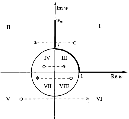
Figure 1: Uniformization plane for the $\pi\pi$ scattering amplitude.

On Fig.1, the Roman numerals (I,II,…,VIII) denote the images of corresponding sheets of the Riemann surface; the thick line represents the physical region (the points $w_{\pi}$, i and 1 are the $\pi\pi$, $K\overline{K}$ and $\eta\eta$ thresholds, respectively). The depicted positions of poles ($*$) and of zeros ($\circ$) give the representation of the type (a) resonance in $S_{11}$. The dashed lines indicate a ”pole-zero” symmetry required for elastic unitarity in the ($w_{\pi}$, i)–region. Here the left-hand cuts are neglected in the Riemann-surface structure, and contributions on these cuts will be taken into account in the background.

The Le Couteur-Newton relations are somewhat modified with taking account of the used model of the Riemann surface (note that on the $w$-plane the points $w_{0}$, $-w_{0}^{-1}$, $-w_{0}$, $w_{0}^{-1}$ correspond to the $s$-variable point $s_{0}$ on sheets I, IV, V, VIII, respectively):

$$S_{11}=\frac{d^{*}(-w^{*})}{d(w)},~{}~{}\qquad S_{22}=\frac{d(-w^{-1})}{d(w)},~{}~{}\qquad S_{33}=\frac{d(w^{-1})}{d(w)},$$ (2)

$$D_{33}=\frac{d^{*}({w^{*}}^{-1})}{d(w)},\qquad D_{22}=\frac{d^{*}(-{w^{*}}^{-1})}{d(w)},\qquad D_{11}=\frac{d(-w)}{d(w)}.$$

Taking the $d$-function as $d=d_{B}d_{res}$ where $d_{B}$, describing the background, is

$$d_{B}=\mbox{exp}[-i\sum_{n=1}^{3}k_{n}(\alpha_{n}+i\beta_{n})],$$

moreover, the $\pi\pi$ background is taken to be elastic up to the $K\overline{K}$ threshold. The resonance part is

$$d_{res}(w)=w^{-\frac{M}{2}}\prod_{r=1}^{M}(w+w_{r}^{*})$$

where $M$ is the number of resonance zeros.

3 Combined analysis of experimental data

We analyzed in a combined way the data on three processes $\pi\pi\to\pi\pi,K\overline{K},\eta\eta$ in the channel with $I^{G}J^{PC}=0^{+}0^{++}$. For the $\pi\pi$-scattering, the data from the threshold to 1.89 GeV are taken from work by B. Hyams et al. [19]; below 1 GeV, from many works [19]. For $\pi\pi\to K\overline{K}$, practically all the accessible data are used [20]. The $|S_{13}|^{2}$ data for $\pi\pi\to\eta\eta$ from the threshold to 1.72 GeV are taken from ref. [22]. As the data, we use the results of phase analyses which are given for phase shifts of the amplitudes and moduli of the $S$-matrix elements.

We obtain a satisfactory description: for the $\pi\pi$-scattering from $\sim$ 0.4 GeV to 1.89 GeV ($\chi^{2}/\mbox{ndf}\approx 1.29$); for the process $\pi\pi\to K\overline{K}$ from the threshold to $\sim$ 1.5 GeV ($\chi^{2}/\mbox{ndf}\approx 2.8$); for the $|S_{13}|^{2}$ data of the reaction $\pi\pi\to\eta\eta$ from the threshold to 1.5 GeV ($\chi^{2}/\mbox{ndf}\approx 0.95$). The total $\chi^{2}/\mbox{ndf}$ for all three processes is 1.95; the number of adjusted parameters is 29. The background parameters (in GeV^-1 units) are $\alpha_{1}=1.51,\beta_{1}=0.0482,\alpha_{2}=-0.93,\beta_{2}=0.139,\beta_{3}=0.89$. On Figures 2, we demonstrate energy dependences of phase shifts and moduli of the matrix elements of processes $\pi\pi\to\pi\pi,K\overline{K},\eta\eta$, compared with the experimental data: $S_{ij}=M_{ij}e^{id_{ij}}$, $D_{13}\equiv M_{13}^{2}$  ($E=\sqrt{s}$).

Figure 2: Comparison of obtained energy dependences with experimental data.

Let us indicate the obtained poles of clusters for resonances on the complex energy plane $\sqrt{s}$, (in MeV units):  for $f_{0}(600)$, type (a): $661\pm 14-i(595\pm 22)$ on sheet II, $649\pm 16-i(595\pm 9)$ on sheet III, $611\pm 17-i(595\pm 28)$ on sheet VI, and $623\pm 15-i(595\pm 26)$ on sheet VI;  for $f_{0}(980)$: $1006\pm 5-i(34\pm 8)$ on sheet II, and $962\pm 18-i(74\pm 20)$ on sheet III;  for $f_{0}(1370)$, type (b): $1384\pm 21-i(50\pm 29)$ on sheet III, $1384\pm 20-i(78\pm 26)$ on sheet IV, $1384\pm 20-i(182\pm 23)$ on sheet V, $1384\pm 20-i(154\pm 25)$ on sheet VI; for $f_{0}(1500)$, type (d): $1505\pm 22-i(320\pm 25)$ on sheet II, $1500\pm 30-i(186\pm 23)$ of the 2nd order on sheet III, $1505\pm 20-i(204\pm 31)$ on sheet IV, $1505\pm 21-i(320\pm 30)$ on sheet V, $1513\pm 28-i(318\pm 27)$ of the 2nd order on sheet VI, and $1505\pm 20-i(204\pm 35)$ on sheet VII;  for $f_{0}(1710)$, type (c): $1699\pm 22-i(179\pm 26)$ on sheet V, $1699\pm 22-i(168\pm 23)$ on sheet VI, $1699\pm 22-i(71\pm 19)$ on sheet VII, and $1699\pm 26-i(82\pm 18)$ on sheet VIII. (To reduce the number of adjusted parameters, we supposed that simple poles of the resonance clusters arise from the simplest 3-channel Breit-Wigner form.)

Note a surprising result obtained for the $f_{0}(980)$ state. It turns out that this state lies slightly above the $K\overline{K}$ threshold and is described by a pole on sheet II and by a shifted pole on sheet III under the $\eta\eta$ threshold without an accompaniment of the corresponding poles on sheets VI and VII, as it was expected for standard clusters. This corresponds to the description of the $\eta\eta$ bound state.

For now, we did not calculate coupling constants in the 3-channel approach, because here rather much variants of combinations of the resonance cluster types are possible and not all the ones are considered to choose the better variant, though already a satisfactory description is obtained. Therefore, for subsequent conclusions, let us mention the results for coupling constants from our previous 2-channel analysis, which have been calculated through the residues of the amplitudes at the poles on the relevant sheets.

Table 3: Coupling constants of the $f_{0}$ states with $\pi\pi$ ($g_{1}$) and $K\overline{K}$ ($g_{2}$) systems. $f_{0}(665)$ $f_{0}(980)$ $f_{0}(1370)$ $f_{0}(1500)$ $g_{1}$, GeV  $0.652\pm 0.065$  $0.167\pm 0.05$  $0.116\pm 0.03$  $0.657\pm 0.113$ $g_{2}$, GeV  $0.724\pm 0.1$  $0.445\pm 0.031$   $0.99\pm 0.05$  $0.666\pm 0.15$

On the basis of the types of pole clusters of the considered resonances and taking into account that (as it is seen from Table 3) the $f_{0}(980)$ and especially the ${f_{0}}(1370)$ are coupled essentially more strongly to the $K\overline{K}$ system than to the $\pi\pi$ one, we have concluded that these states have a dominant $s{\bar{s}}$ component. The $f_{0}(1500)$ has the approximately equal coupling constants with the $\pi\pi$ and $K\overline{K}$ systems, which apparently could point up to its dominant glueball component. In the 2-considerations, $f_{0}(1710)$ is represented by the pole cluster corresponding to a state with the dominant $s{\bar{s}}$ component.

Our 3-channel conclusions on the basis of resonance cluster types generally confirm the ones drawn in the 2-channel analysis, besides the above surprising conclusion about the $f_{0}(980)$ nature.

Masses and widths of these states should be calculated from the pole positions. If we take the resonance part of amplitude as

$$T^{res}=\frac{\sqrt{s}\Gamma_{el}}{m_{res}^{2}-s-i\sqrt{s}\Gamma_{tot}},$$

we obtain for masses and total widths the following values (in MeV units): for $f_{0}(665)$, 889 and 1190; for $f_{0}(980)$, 1006 and 64; for $f_{0}(1370)$, 1386 and 156; for $f_{0}(1500)$, 1539 and 640; for $f_{0}(1710)$, 1701 and 164.

4 Lower scalar $0^{++}$ nonets

Although at present many states have been discovered in the scalar mesonic sector [1], however, their assignment to quark-model configurations is problematic – one can compare various variants of that assignment, for example, [23]-[28].

On the basis of obtained results, we can propose a following assignment of scalar mesons below 1.9 GeV to lower nonets. First of all, we exclude from this consideration the $f_{0}(980)$ as the $\eta\eta$ bound state. Then we propose to include to the lowest nonet the isovector $a_{0}(980)$, the isodoublet $K_{0}^{*}(900)$ (or $\kappa(800)$), and two isoscalars $f_{0}(600)$ and $f_{0}(1370)$ as mixtures of the eighth component of octet and the SU(3) singlet. Note also that we consider the $K_{0}^{*}(900)$ (or $\kappa$), observed at analysing the $K-\pi$ scattering [29] and at studying the decay $D^{+}\to K^{-}\pi^{+}\pi^{+}$ (Fermilab experiment E791) [30]. Then the Gell-Mann–Okubo formula

$$3m_{f_{8}}^{2}=4m_{K^{*}}^{2}-m_{a_{0}}^{2}$$ (3)

gives $m_{f_{8}}=0.87$ GeV. Our result for the $\sigma$-meson mass is $m_{\sigma}\approx 0.889\pm 0.02$ GeV (if $m_{\kappa}=0.8$, $m_{f_{8}}\approx 0.73$).

The second relation for masses of nonet, which is obtained only on basis of the quark contents of the nonet members and somehow restricts mass of the SU(3) singlet, is

$$m_{\sigma}+m_{f_{0}(1370)}=2m_{\kappa}.$$ (4)

The left-hand side of this relation is $\sim$ 25 % bigger than the right-hand one if to take our mass values.

The next nonet could be formed of the isovector $a_{0}(1450)$, the isodoublet $K_{0}^{*}(1430-1450)$, and of the $f_{0}(1500)$ and $f_{0}(1710)$ as mixtures of the eighth component of octet (mixed with a glueball) and the SU(3) singlet. From the Gell-Mann–Okubo formula we obtain $m_{f_{8}}\approx 1.45$ GeV. In second formula

$$m_{f_{0}(1500)}+m_{f_{0}(1710)}=2m_{K^{*}(1450)},$$ (5)

the left-hand side is $\sim$ 12 % bigger than the right-hand one.

Though the Gell-Mann–Okubo formula is fulfilled for both nonets rather satisfactorily, however, the breaking of 2nd relation (especially for the lowest nonet) tells us that the $\sigma-f_{0}(1370)$ and $f_{0}(1500)-f_{0}(1710)$ systems get additional contributions absent in the $K_{0}^{*}(900)$ and $K_{0}^{*}(1450)$, respectively.

5 Conclusions

• In a combined model-independent analysis of data on the $\pi\pi$ scattering from 0.4 to 1.89 GeV and processes $\pi\pi\to K\overline{K},\eta\eta$ from the thresholds to 1.5 GeV, a confirmation of the $\sigma$-meson with mass 0.889 GeV is obtained once more. This mass value rather accords with prediction ($m_{\sigma}=m_{\rho}$) on the basis of mended symmetry by Weinberg [31].

• Consideration of the $\eta\eta$ channel is necessary for a consistent and reasonable representation of the obtained resonances. For satisfactory description of the processes $\pi\pi\to K\overline{K},\eta\eta$ above $\sim$ 1.5 GeV, an allowance for channels (first of all, the $\eta\eta^{\prime}$ one) opening in this region is necessary.

• The $f_{0}(980)$, ${f_{0}}(1370)$ and $f_{0}(1710)$ have the dominant $s{\bar{s}}$ component. Moreover, we obtain an additional indication for $f_{0}(980)$ to be the $\eta\eta$ bound state. Remembering a dispute [32] whether the $f_{0}(980)$ is narrow or not, we agree rather with the former. Of course, it is necessary to make analysis of other relevant processes, first of all, $J/\psi$ and $\phi$ decays. Note also that our conclusion about the large $s{\bar{s}}$ component for the $f_{0}(1710)$ quite is consistent with the experimental facts that this state is observed in $\gamma\gamma\to K_{S}K_{S}$ [33] and not observed in $\gamma\gamma\to\pi^{+}\pi^{-}$ [34].

• As to the $f_{0}(1500)$, we suppose that it is practically the eighth component of octet mixed with a glueball being dominant in this state.

• An assignment of the scalar mesons below 1.9 GeV to lower nonets is proposed. Note that this assignment moves a number of questions and does not put the new ones. It is clear that now an adeguate mixing scheme should be found.

ACKNOWLEDGEMENTS - This work has been supported by the Grant Program of Plenipotentiary of Slovak Republic at JINR. M.N. were supported in part by the Slovak Scientific Grant Agency, Grant VEGA No. 2/3105/23; and D.K., by Grant VEGA No. 2/5085/99.

References

- [1] K. Hagiwara et al., Phys. Rev. D 1166, 010001 (2002).
- [2] Yu.S. Surovtsev, D. Krupa, and M. Nagy, Eur. Phys. J. A 15, 409 (2002).
- [3] R.L. Jaffe and C.L. Korpa, Comm. Nucl. Part. Phys. 17, 163 (1987); J. Gasser, H. Leutwyler, and M.E. Sainio, Phys. Lett. 253, 252 (1991); T. Hatsuda and T. Kunihiro, Nucl. Phys. B 387, 715 (1992); M. Nagy, N.L. Russakovich, and M.K. Volkov, Acta Physica Slovaca 51, 299 (2001).
- [4] E.P. Shabalin, Sov. J. Nucl. Phys. 48, 172 (1988); T. Morozumi, C.S. Lim, and A.I. Sanda, Phys. Rev. Lett. 65, 404 (1990); J.C.R. Bloch et al., Phys. Rev. C 62, 025206 (2000).
- [5] K. Holinde, Phys. Rep. 68, 121 (1981).
- [6] N.A. Törnqvist and M. Roos, Phys. Rev. Lett. 76, 1575 (1996).
- [7] V.V. Anisovich, D.V. Bugg, and A.V. Sarantsev, Phys. Rev. D 58, 111503 (1998).
- [8] B.S. Zou and D.V. Bugg, Phys. Rev. D 48, R3948 (1993); ibid. 50, 591 (1994).
- [9] M. Svec, Phys. Rev. D 53, 2343 (1996).
- [10] S. Ishida et al., Progr. Theor. Phys. 95, 745 (1996); ibid. 98, 621 (1997).
- [11] R. Kamiński, L. Leśniak, and B. Loiseau, Eur. Phys. J. C 9, 141 (1999).
- [12] Yu.S. Surovtsev, D. Krupa, and M. Nagy, Phys. Rev. D 63, 054024 (2001) 054024.
- [13] L. Li, B.-S. Zou, and G.-lie Li, Phys. Rev. D 63, 074003 (2001).
- [14] P. Minkowski and W. Ochs, hep-ph/0209225.
- [15] N.N. Achasov and G.N. Shestakov, Phys. Rev. D 49, 5779 (1994).
- [16] D. Krupa, V.A. Meshcheryakov, and Yu.S. Surovtsev, Nuovo Cim. A 109, 281 (1996).
- [17] D. Morgan and M.R. Pennington, Phys. Rev. D 48, 1185 (1993).
- [18] K.J. Le Couteur, Proc. Roy. Soc. A 256, 115 (1960); R.G. Newton, J. Math. Phys. 2, 188 (1961); M. Kato, Ann. Phys. 31, 130 (1965).
- [19] B. Hyams et al., Nucl. Phys. B 64, 134 (1973); ibid. 100, 205 (1975); A. Zylbersztejn et al., Phys. Lett. B 38, 457 (1972); P. Sonderegger and P. Bonamy, in Proc. 5th Intern. Conf. on Elementary Particles, Lund, 1969, paper 372; J.R. Bensinger et al., Phys. Lett. B 36, 134 (1971); J.P. Baton et al., Phys. Lett. B 33, 525, 528 (1970); P. Baillon et al., Phys. Lett. B 38, 555 (1972); L. Rosselet et al., Phys. Rev. D 15, 574 (1977); A.A. Kartamyshev et al., Pis’ma v Zh. Eksp. Teor. Fiz. 25, 68 (1977); A.A. Bel’kov et al., Pis’ma v Zh. Eksp. Teor. Fiz. 29, 652 (1979).
- [20] W. Wetzel et al., Nucl. Phys. B 115, 208 (1976); V.A. Polychronakos et al., Phys. Rev. D 19, 1317 (1979); P. Estabrooks, Phys. Rev. D 19, 2678 (1979); D. Cohen et al., Phys. Rev. D 22, 2595 (1980); G. Costa et al., Nucl. Phys. B 175, 402 (1980); A. Etkin et al., Phys. Rev. D 25, 1786 (1982).
- [21] C. Amsler and F.E. Close, Phys. Rev. D 53, 295 (1996).
- [22] F. Binon et al., Nuovo Cim. A 78, 313 (1983).
- [23] J. Lánik, Phys. Lett. B 306, 139 (1993).
- [24] N.A. Törnqvist, hep-ph/0204215.
- [25] V.V. Anisovich, Yu.D. Prokoshkin and A.V. Sarantsev, Nucl. Phys. Proc. Suppl. A56, 270 (1997).
- [26] F.E. Close and N.A. Törnqvist, J. Phys. G 28, R249 (2002).
- [27] P. Minkowski and W. Ochs, hep-ph/0209223.
- [28] M.K. Volkov and V.L. Yudichev, Yad. Fiz. 65, 1701 (2002).
- [29] S. Ishida et al., Prog. Theor. Phys. 98, 621 (1997).
- [30] C. Gobel et al. (E791 Collaboration), hep-ex/0204018.
- [31] S. Weinberg, Phys. Rev. Lett. 65, 1177 (1990).
- [32] B.S. Zou and D.V. Bugg, Phys. Rev. D 48, R3948 (1993); D. Morgan and M.R. Pennington, Phys. Rev. D 48, 5422 (1993).
- [33] S. Braccini, Proc. Workshop on Hadron Spectroscopy, Frascati Physics Series XV, 53 (1999).
- [34] R. Barate et al., Phys. Lett. B 472, 189 (2000).