Abstract

We calculate the cosmic microwave background (CMB) anisotropy spectrum in models with millicharged particles of electric charge $q\sim 10^{-6}-10^{-1}$ in units of electron charge. We find that a large region of the parameter space for the millicharged particles exists where their effect on the CMB spectrum is similar to the effect of baryons. Using WMAP data on the CMB anisotropy and assuming Big Bang nucleosynthesis value for the baryon abundance we find that only a small fraction of cold dark matter, $\Omega_{mcp}h_{0}^{2}<0.007$ (at 95% CL), may consists of millicharged particles with the parameters (charge and mass) from this region. This bound significantly narrows the allowed range of the parameters of millicharged particles. In models without paraphoton millicharged particles are now excluded as a dark matter candidate. We also speculate that recent observation of 511 keV $\gamma$-rays from the Galactic bulge may be an indication that a (small) fraction of CDM is comprised of the millicharged particles.

Search for particles carrying small but non-vanishing electric charge (millicharged particles) has long history. If observed, millicharged particles would either cause serious doubts on the concept of Grand Unification or imply the existence of a new massless gauge boson — paraphoton [1, 2]. Furthermore, the existence of millicharged particles would hint towards processes with apparent electric charge non-conservation, like electron or proton decay to “nothing” [3].

There are various constraints on the parameters (charge and mass) of millicharged particles, coming from collider and laboratory experiments and from cosmology and astrophysics (see, e.g., Refs. [4, 5, 6, 7, 8, 9] for the latest results and Refs. [10, 11] for reviews), see Fig. 1. Interestingly, reported bounds did not exclude a possibility [12] that a significant part (or even all) of the cold dark matter (CDM) is comprised of millicharged particles.

The constraints on the parameters of millicharged particles are somewhat different in theories with and without paraphoton. Without paraphoton, two domains in the parameter space of millicharged particles are allowed. The first one corresponds to heavy particles with tiny electric charge (left upper corner in Fig. 1) which would never be produced thermally in the early Universe. This region is far beyond the reach of future collider and laboratory experiments. In the current Letter we are concerned with another region. This is a narrow window of relatively light particles with masses $M\sim 10^{-3}\div 10^{2}$ GeV and charges $q\sim 10^{-6}\div 10^{-1}$. Larger charges $q\gtrsim 0.1$ are ruled out by limits on the cosmic ray fluxes of fractionally charged particles [11]. It is worth noting that particles with $q\gtrsim 0.2$ are also excluded by measurements of the width of Z-boson (cf. Ref. [5]) if one makes use of the latest data [13].

In model with paraphoton, and for not very small values of the paraphoton coupling constant $\alpha^{\prime}$, millicharged particles annihilate mainly into pairs of paraphotons. As a result, their annihilation in the early Universe is more efficient and the cosmological bound coming from the relic abundance depends on the value of $\alpha^{\prime}$ and generically is less restrictive (see Fig. 1) than in the model without paraphoton.

It was noted in Ref. [14], that there is a part of the parameter space for the millicharged particles where they do not decouple from the acoustic oscillations of the baryon-photon plasma at recombination, and it was suggested that the effect of these particles on the CMB anisotropy spectrum may be similar to the effect of baryons. The purpose of this Letter is, using the recent precise CMB data from WMAP [15], to set an upper limit on the fraction of millicharged particles in CDM and to narrow the allowed window for millicharged particles. Assuming the standard Big Bang nucleosynthesis (BBN) value for the baryon abundance, $\Omega_{b}h_{0}^{2}=0.0214\pm 0.0020$ [16], we arrive at the following constraint on the millicharged particle abundance,

$$\Omega_{mcp}h_{0}^{2}<0.007\;\;(95\%~{}{\rm CL})\;,$$ (1)

if millicharged particles are coupled to baryons at recombination. The latter condition is satisfied on the right of the dark solid line in Fig. 1. We see that the upper limit (1) apllies in the whole allowed window for millicharged particles in models without paraphoton. It is also worth stressing that in models with paraphoton the domain of applicability of the upper bound (1) does not depend on the value of $\alpha^{\prime}$. Using the Lee-Weinberg formula [17] for the relic abundance one then translates the upper bound (1) into the lower limit on the annihilation cross section of millicharged particles. As a result, the upper bound (1) excludes most part of the allowed window for the millicharged particles in models without paraphoton, leaving a small allowed region with masses in the range $m\sim 10^{-1}-10$ GeV and charges in the range $q\sim 10^{-3}-10^{-1}$. In models with paraphoton, the bound (1) translates into meaningful limit on the parameters of millicharged particles as shown in Fig. 1; the excluded region depends on the value of $\alpha^{\prime}$.

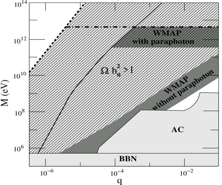
Figure 1: The exclusion plot in the parameter space for millicharged particles. Light grey area is excluded by accelerator experiments and BBN. Dashed region is excluded by the relic abundance of millicharged particles in models without paraphoton. Part of this region above the dash-dotted line is excluded by the relic abundance in models with paraphoton (assuming $\alpha^{\prime}=0.1$). On the left of the dotted line millicharged particles cannot be thermally produced in the Early Universe. Dark grey and dashed dark grey areas are the previously allowed regions which are now excluded by Eq. (1) in models without and with paraphoton, respectively. On the right of the dark solid line millicharged particles are coupled to baryons (see Eq. (8) in the text).

Let us proceed to the derivation of the upper bound (1). To calculate the CMB anisotropy spectrum we adapt the CMBFAST code [18] which solves numerically the set of kinetic equations [19] for the linear perturbations in the primordial plasma. To take into account the presence of millicharged particles we extend this set by adding the kinetic equations for the millicharged component, modify the equations for the baryon component to take into account the elastic scattering off millicharged particles and include millicharged component contribution to the energy-momentum tensor. The rest of the perturbation equations are the same as in Ref. [19]. The Compton scattering off millicharged particles is negligible, since the corresponding cross section is suppressed by the fourth power of the charge $q$.

We work in synchronous gauge and consider primordial plasma in the expanding Universe with scale factor $a(\tau)$ (where $\tau$ is a conformal time) normalized to unity at present time. Let $T_{f}$, $\rho_{f}$, $\vec{v}_{f}$ be the temperature, density and velocity of the $f$-th component of the plasma. In particular, $f=e,b,\gamma,mcp$ for electrons, baryons, photons and millicharged particles, respectively. In what follows bar denotes space averaging. The standard variables describing fluid perturbations are $\delta_{f}(\vec{k},\tau)=[\rho_{f}(\vec{k},\tau)-\bar{\rho}_{f}(\tau)]/\bar{\rho}_{f}(\tau)$ and $\theta_{f}(\vec{k},\tau)=ik_{j}v_{f}^{j}(\vec{k},\tau)$ where $k_{i}$ is conformal momentum.

Before recombination, the interaction between non-relativistic electrons and protons is strong enough to ensure that electron and baryon components have equal velocities, $\theta_{e}=\theta_{b}$. This makes it possible to use tight coupling approximation and consider electrons and protons as single baryon fluid [20]. Then the set of equations for baryons and millicharged particles reads (cf. Ref. [19])

$$\dot{\delta}_{b} =-\theta_{b}-\frac{1}{2}\dot{h},$$

$$\dot{\theta}_{b} =-\frac{\dot{a}}{a}\theta_{b}+c_{s}^{2}k^{2}\delta_{b}+\frac{4\bar{\rho}_{\gamma}}{3\bar{\rho}_{b}}an_{e}\sigma_{T}(\theta_{\gamma}-\theta_{b})$$

$$+a\Gamma_{mcp}\Omega_{mcp}(\theta_{mcp}-\theta_{b}),$$ (2)

$$\dot{\delta}_{mcp} =-\theta_{mcp}-\frac{1}{2}\dot{h},$$

$$\dot{\theta}_{mcp} =-\frac{\dot{a}}{a}\theta_{mcp}+c_{s,mcp}^{2}k^{2}\delta_{mcp}$$

$$+a\Gamma_{mcp}\Omega_{b}(\theta_{b}-\theta_{mcp}),$$ (3)

where $h$ is the longitudinal metric perturbation, dot stands for derivative with respect to the conformal time $\tau$; $c_{s}$, $c_{s,mcp}$ are the sound velocities in the baryon and millicharged components, $n_{e}$ is the number density of electrons and $\Gamma_{mcp}$ is the velocity transfer rate for millicharged particles due to scattering off baryons and electrons. The latter is given by

$$\Gamma_{mcp}=\sum\limits_{x=e,p}\frac{n_{x}}{\Omega_{b}}\left.\frac{\partial}{\partial v_{M,x}}\left<\int\Delta v_{M}\cdot d\sigma_{M,x}\right>\right|_{v_{M,x}=0},$$ (4)

where brackets stand for thermal averaging, $v_{M,e(p)}$ is relative velocity and $\Delta v_{M}$ is velocity transfer in a single process of scattering; $d\sigma_{M,e}$ ($d\sigma_{M,p}$) is the Rutherford cross section for millicharged particles scattering off electron (proton).

The Rutherford cross section is singular at zero scattering angle, but due to Debye screening the integral in Eq. (4) is cut at the value of the scattering angle equal to the Debye angle, $\theta_{D}=\sqrt{2\pi\alpha n_{e}/T^{2}m_{e}}$. As a result one arrives at the following expression for the velocity transfer rate in the case of thermal equilibrium

$$\Gamma_{mcp}=\frac{4\sqrt{2\pi}\alpha^{2}q^{2}\rho_{crit}}{3Mm_{p}a^{3/2}(\tau)T_{0}^{3/2}}|\ln\theta_{D}|(\sqrt{\mu_{M,e}}+\sqrt{\mu_{M,p}})\;,$$ (5)

where $\mu_{M,e(p)}$ is the reduced mass of a millicharged particle and electron (proton), $\alpha$ is the fine structure constant and $T_{0}\approx 2.726$ K is the present CMB temperature. It is straightforward to generalize Eq. (5) to nonequilibrium case when electrons, protons and millicharged particles have different temperatures. In that case the value of $\Gamma_{mcp}$ is larger than the one given by Eq. (5), so Eq. (5) may be used as a lower estimate of the interaction rate, which is sufficient for our purposes.

We solve the system of the kinetic equations starting from the early moment of time $\tau_{i}$ and using inflationary initial conditions [19],

$$\delta_{mcp} =\delta_{b}=\frac{3}{4}\delta_{\gamma}=-\frac{1}{2}C(k\tau_{i})^{2},$$

$$\theta_{mcp} =\theta_{\gamma}=\theta_{b}=-\frac{1}{18}Ck(k\tau_{i})^{3}\;,$$

where constant $C$ determines the overall normalization.

The last terms in the r.h.s. of Eqs. (2), (3) tend to equalize the velocities of the baryon and millicharged components of the fluid. This results in the kinetic equilibrium, $\theta_{mcp}=\theta_{b}$, provided $\Gamma_{mcp}$ is large enough. In this case, the perturbation equations are difficult to solve numerically, because the kinetic relaxation rate for the interaction of millicharged particles and baryons is much larger than the rates of other processes. To deal with this situation we make use of the zeroth order tight coupling approximation adopting the method of Peebles and Yu [20]. Namely, we expand Eqs. (2), (3) to the zeroth order in $\Gamma_{mcp}^{-1}$, setting $\theta_{b}=\theta_{mcp}=\theta$. Then we exclude $\Gamma_{mcp}$ from Eqs. (2), (3) and arrive at the following equation

$$\dot{\theta}= -\frac{\dot{a}}{a}\theta+\frac{\Omega_{b}}{\Omega_{b}+\Omega_{mcp}}\frac{4\bar{\rho}_{\gamma}}{3\bar{\rho}_{b}}an_{e}\sigma_{T}(\theta_{\gamma}-\theta)$$ (6)

$$+\frac{\Omega_{b}~{}c_{s}^{2}\delta_{b}+\Omega_{mcp}~{}c_{s,mcp}^{2}\delta_{mcp}}{\Omega_{b}+\Omega_{mcp}}k^{2}\;.$$

The CMB spectrum obtained in this approximation agrees with the solution of the original set of equations at the level of one percent provided that

$$\Gamma_{mcp}(\tau_{rec})(\Omega_{b}+\Omega_{mcp})H(\tau_{rec})^{-1}\gtrsim 250\;,$$ (7)

where $\tau_{rec}$ is conformal time at recombination and $H(\tau_{rec})$ is the Hubble parameter. In what follows we discuss a region of parameters where tight coupling condition (7) is satisfied (in particular, this region covers the whole allowed window in models without paraphoton) and comment on the rest of the parameter space in due course.

To compare the results of our simulation with the CMB data we consider the flat $\Lambda$CDM model with the number of massless neutrino species $N_{\nu}=3$. We perform a scan over the space of the cosmological models by varying parameters from minimal to maximal values as given in Table 1. All priors are at 95% CL.

$parameter$	$min.~{}value$	$max.~{}value$	$step$	reference
$\Omega_{C\!D\!M}$	0.2	0.4	0.01	PDG [13]
$h_{0}$	0.64	0.79	0.01	PDG [13]
$n_{s}$	0.8	1.2	0.01
$\Omega_{b}h_{0}^{2}$	0.0194	0.0234	0.0005	BBN [16]
$\Omega_{mcp}$	0	0.020	0.001

Table 1: The ranges of the cosmological parameters used in simulations; we never have a good fit outside the region $n_{s}\in[0.8,1.2]$, and for $\Omega_{mcp}>0.02$.

We assume helium fraction at the moment of recombination $Y_{He}=0.24$. We have checked that reionization effects are irrelevant here, the reason being that reionization affects the spectrum only at the lowest values of the multipole moments.

For each cosmological model we calculated likelihood to the WMAP data [15]. As a result we arrived at the limit given by Eq. (1), which means that no model exists in the considered parameter range with larger values of $\Omega_{mcp}h_{0}^{2}$ and likelihood better than 5%. We also checked that additional CMB data from CBI [21] and ACBAR [22] do not improve the limit (1).

Using the Lee–Weinberg formula we translate the limit given by Eq. (1) into the bound on the parameter space. The corresponding excluded areas are shown in Fig. 1. In models with paraphoton we extend our analysis to the region where the tight coupling condition (7) is not satisfied. We checked that actually the upper bound (1) applies provided that the following less restrictive condition holds

$$\Gamma_{mcp}(\tau_{rec})(\Omega_{b}+\Omega_{mcp})H(\tau_{rec})^{-1}\gtrsim 2.5\;.$$ (8)

This inequality is true on the right of the black solid line in Fig. 1.

Coming back to the tight coupling regime, let us illustrate the upper bound (1) pictorially by generating a set of models with random parameters in tight coupling regime, assuming uniform distribution of models in the parameter space within ranges given in Table 1. For each model we calculated likelihood to the observed CMB spectrum and plot the resulting distribution of models in the ($\Omega_{b}h_{0}^{2}$, $\Omega_{mcp}h_{0}^{2}$) plane in Fig. 2.

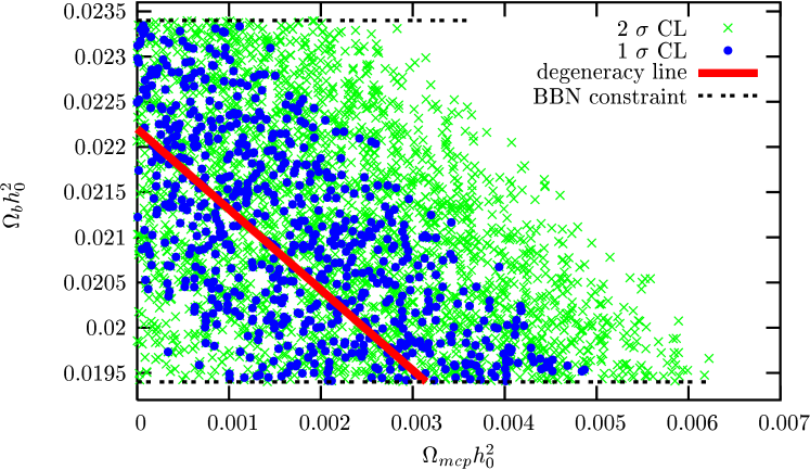
Figure 2: Distribution of models in the ($\Omega_{b}h_{0}^{2}$, $\Omega_{mcp}h_{0}^{2}$) plane. Crosses and dots denote models agreeing with data at the 2$\sigma$ and 1$\sigma$ CL, respectively. The bold line illustrates the degeneracy of the CMB anisotropy spectrum. Two dotted lines show the range of $\Omega_{b}h_{0}^{2}$ allowed by BBN.

One observes that the CMB spectrum is approximately degenerate along the straight line

$$\Omega_{b}h_{0}^{2}=0.022-1.1~{}\Omega_{mcp}h_{0}^{2}.$$ (9)

This degeneracy is in agreement with the expectation of Ref. [14], that the effect of millicharged particles is similar to that of baryons. Thus in models with millicharged particles, the CMB data [15] determine actually the sum $(\Omega_{b}+\Omega_{mcp})h_{0}^{2}=0.022\pm 0.001$ (68% CL). Combining this value with the lower limit $\Omega_{b}h_{0}^{2}>0.019$ from BBN one arrives at the upper bound very similar to Eq. (1). This serves as a qualitative explanation of our result.

Another illustration of the approximate degeneracy (9) is shown in Fig. 3, where two CMB anisotropy spectra calculated for different models on the degeneracy line are shown. One observes that the two spectra almost coincide in the region of the first and second acoustic peaks. However, the degeneracy is no longer present at higher multipoles. This is due to the fact that the electroneutrality of the plasma implies that the electron number density is proportional to the baryon density. Hence, replacing a certain amount of baryons by millicharged particles results in the enhancement of the Silk damping at small scales.

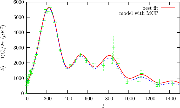
Figure 3: Two different CMB anisotropy spectra compared with extended WMAP dataset. Solid line represents the best fit model without millicharged particles, $\Omega_{b}h_{0}^{2}=0.022$. Dashed line corresponds to model with $\Omega_{b}h_{0}^{2}=0.014,\Omega_{mcp}h_{0}^{2}=0.007$.

With future precise data for high values of $l$, one will be able to set a constraint on the value of $\Omega_{mcp}$ using the CMB data only, without reference to BBN results. To check this we created a simulated dataset, which contains the same values of $l$ as in the WMAP data up to $l=500$, and then with the step $\Delta l=50$ up to $l=1600$. The CMB anisotropy spectral coefficients $C_{l}$’s were taken from the best fit [15] to WMAP data. The error bars for these coefficients were assumed to be equal to cosmic variance. Repeating the above procedure for this dataset we obtained that an upper limit $\Omega_{mcp}h_{0}^{2}<0.003$ can be placed. Further improvement of this limit turns out to be impossible due to the new approximate degeneracy,

$$\Omega_{b}h_{0}^{2}=0.022-0.65~{}\Omega_{mcp}h_{0}^{2}\;,$$

$$n_{s}=0.94+8.0~{}\Omega_{mcp}\;,$$ (10)

arising at smaller values of $\Omega_{mcp}h_{0}^{2}$.

To conclude, we note that when translated into the parameter space, the limit (1) is especially interesting for the models without paraphoton, where it excludes most part of the window with not very heavy particles and substantial electric charges. To completely close the window, sensitivity to millicharged particle abundance at the level of $\Omega_{mcp}h_{0}^{2}\sim 3\cdot 10^{-4}$ would be required, which cannot be achieved with future CMB experiments due to the degeneracy (10). Determination of the baryon abundance from the BBN is not accurate enough to improve the situation. Hopefully, the rest of the window will be explored by future accelerator and/or laboratory experiments.

Finally, recently it was suggested [23] that the flux of the 511 keV $\gamma$-rays from the Galactic bulge detected by the INTEGRAL satellite [24] may be explained by the annihilation of the $\sim 1\div 100$ MeV dark matter particles into $e^{+}e^{-}$ pairs, provided their annihilation cross section $\sigma\beta$ and abundance $\Omega$ satisfy $\left(\frac{\sigma\beta}{\rm{pb}}\right)\left(\frac{1\rm{MeV}}{M}\right)^{2}\left(\frac{\Omega^{2}}{\Omega^{2}_{C\!D\!M}}\right)\simeq 10^{-(3.5\div 4.5)}$. Intriguingly, this condition holds in the left corner of the parameter space for millicharged particles without paraphoton allowed by Eq. (1) (say, for $q=3\cdot 10^{-3}$, $M=100$ MeV). One is tempted to speculate that the observation of the 511 keV line is an indication that a (small) fraction of CDM is comprised of the millicharged particles. This possibility will be checked by the future CMB data.
Acknowledgments. We would like to thank V.Rubakov and S.Sibiryakov for useful discussions. This work was supported in part by the RFBR02-02-17398 and GPRFNS-2184.2003.2 grants. The work of D.G. was also supported in part by the GPRF grant MK-2788.2003.02.

References

- [1] L. B. Okun, M. B. Voloshin and V. I. Zakharov, Phys. Lett. B 138, 115 (1984).
- [2] B. Holdom, Phys. Lett. B 166, 196 (1986).
- [3] A. Y. Ignatev, V. A. Kuzmin and M. E. Shaposhnikov, Phys. Lett. B 84, 315 (1979).
- [4] M. I. Dobroliubov and A. Y. Ignatev, Phys. Rev. Lett. 65, 679 (1990).
- [5] S. Davidson, B. Campbell and D. C. Bailey, Phys. Rev. D 43, 2314 (1991).
- [6] S. Davidson and M. E. Peskin, Phys. Rev. D 49, 2114 (1994) [arXiv:hep-ph/9310288].
- [7] A. A. Prinz et al., Phys. Rev. Lett. 81, 1175 (1998).
- [8] R. N. Mohapatra and I. Z. Rothstein, Phys. Lett. B 247, 593 (1990).
- [9] R. N. Mohapatra and S. Nussinov, Int. J. Mod. Phys. A 7, 3817 (1992).
- [10] S. Davidson, S. Hannestad, and G. Raffelt, JHEP 05,003(2000).
- [11] M. L. Perl, et al., Int. J. Mod. Phys. A 16, 2137 (2001).
- [12] H. Goldgberg and L.J. Hall, Phys. Lett. B 174, 151 (1986).
- [13] K. Hagiwara et al. [Particle Data Group Collaboration], Phys. Rev. D 66, 010001 (2002).
- [14] S.L. Dubovsky and D.S. Gorbunov, Phys. Rev. D 64, 123503 (2001).
- [15] D. N. Spergel et al., Astrophys. J. Suppl. 148, 175 (2003).
- [16] D. Kirkman, et al., [arXiv:astro-ph/0302006].
- [17] B. W. Lee and S. Weinberg, Phys. Rev. Lett. 39, 165 (1977).
- [18] U. Seljak and M. Zaldarriaga, Astrophys. J. 469, 437 (1996), http://www.cmbfast.org/
- [19] C.-P. Ma and E. Bertschinger, Astrophys. J. 455, 7 (1995)
- [20] P.J.E. Peebles and J.T. Yu, Astrophys. J.162, 816 (1970).
- [21] T. J. Pearson et al., Astrophys. J. 591, 556 (2003).
- [22] C. l. Kuo et al. [ACBAR collaboration], [arXiv:astro-ph/0212289].
- [23] C. Boehm, D. Hooper, J. Silk and M. Casse, arXiv:astro-ph/0309686.
- [24] J. Knodlseder et al., arXiv:astro-ph/0309442; P. Jean et al., Astron. Astrophys. 407, L55 (2003).