YERPHI-1588(9)

Complete bremsstrahlung corrections to the forward-backward asymmetries in $b\rightarrow X_{s}\ell^{+}\ell^{-}$

H. M. Asatrian, H. H. Asatryan, A. Hovhannisyan, V. Poghosyan
Yerevan Physics Institute, 2 Alikhanyan Br., 375036, Yerevan, Armenia

In a recent paper we presented a calculation of NNLL virtual corrections to the forward-backward asymmetries in $b\rightarrow X_{s}\ell^{+}\ell^{-}$ decay. That result does not include bremsstrahlung corrections which are free from infrared and collinear singularities. In the present paper we include the remaining ${\cal O}(\alpha_{s})$ bremsstrahlung corrections to the forward-backward asymmetries in $b\rightarrow X_{s}\ell^{+}\ell^{-}$ decay. The numerical effect of the calculated contributions is found to be below 1%.

1 Introduction

Rare B-decays are known to provide a unique source of information about the physics at the scales of several hundred GeV. In the standard model (SM) all these decays proceed through loop diagrams and are suppressed. Thus in the extensions of the SM the contributions from the ’new’ sources of flavor-violation can be comparable to or even larger than the SM contribution. Therefore experimental information on rare decays can be used to test the SM at the one-loop level or to put constraints on its extensions.

During the last decade the experimental and theoretical efforts were concentrated on the $b\to s\gamma$ mediated decays. Available experimental data already provides stringent constraints on certain extensions of the SM. In 2002, also the exclusive $B\rightarrow K_{s}\mu^{+}\mu^{-}$ decay mode was measured by the BELLE collaboration [1]. This measurement was confirmed soon by the BABAR Collaboration [2]. Recently, also the first measurement of the branching ratio in the inclusive decay $B\rightarrow X_{s}\ell^{+}\ell^{-}$ has been reported by the BELLE Collaboration [3]. The results of these first measurments are compatible with SM predictions though more statistics will be needed for more decisive conclusions. It is expected that precise measurement of kinematical distributions for the $B\rightarrow X_{s}\ell^{+}\ell^{-}$ decay combined with data on $B\rightarrow X_{s}\gamma$ will significantly tighten the constraints on the extensions of the standard model [4].

¿From the theoretical point of view the description of $B\rightarrow X_{s}\ell^{+}\ell^{-}$ decay is problematic because of the long-distance contributions from intermediate $c\bar{c}$ resonant states. When the invariant mass $\sqrt{s}$ of lepton pair is close to the mass of resonance, only model dependent predictions for these long distance contributions are available today. However for the region $0.05<\hat{s}=s/m_{b}^{2}<0.25$ the nonperturbative effects are estimated to be below 10% [5]-[10] and the differential decay rate for $B\rightarrow X_{s}\ell^{+}\ell^{-}$ can be well approximated by HQET corrected short distance contribution.

The next-to-leading logarithmic (NLL) calculation for $B\rightarrow X_{s}\ell^{+}\ell^{-}$ has been performed quite long ago in [11, 12]. However those results are known to suffer from a relatively large ($\pm 16\%$) dependence on the matching scale $\mu_{W}$. The NNLL corrections to the Wilson coefficients eliminate the matching scale dependence to a large extent [13], but leave a $\pm 13\%$-dependence on the renormalization scale $\mu_{b}$, which is of order ${\cal O}(m_{b})$. To further improve the theoretical prediction, ${\cal O}(\alpha_{s})$ virtual and bremsstrahlung corrections have been calculated [14]-[16]. As a result the renormalization scale dependence reduced by a factor of 2.

It is well known that the measurement of the forward-backward asymmetries for decay $B\rightarrow X_{s}\ell^{+}\ell^{-}$ can be used, in combination with the measurement of $B\rightarrow X_{s}\gamma$, to perform a so-called model independent test of the standard model [4], [17],[18]. The double differential decay width $d\Gamma/[d\hat{s}dcos{\theta}]$ and the forward-backward asymmetries have recently been calculated with NNLL precision [19],[20]. Those calculations included one-loop virtual ${\cal O}(\alpha_{s})$ corrections associated with the operators $O_{7}$, $O_{9}$ and $O_{10}$ as well as the corresponding bremsstrahlung corrections that are necessary to cancel the infrared and mass singularities. It was found that NNLL corrections drastically reduce the renormalization scale dependence of forward-backward asymmetries. In the present paper we complete the calculation of the NNLL calculation for the forward-backward asymmetries, presenting the full results for the bremsstrahlung corrections associated with the operators $O_{1}$, $O_{2}$, $O_{8}$ which were omitted in [19],[20].

The paper is organized as follows. In section 2 we briefly describe the theoretical framework. In section 3 the analytical results for the forward-backward asymmetries in $b\rightarrow X_{s}\ell^{+}\ell^{-}$ decay are presented. In section 4 we discuss the technical details of the calculations and give phenomenological analysis for the forward-backward asymmetries in $b\rightarrow X_{s}\ell^{+}\ell^{-}$ decay .

2 The Theoretical Framework

The most efficient tool for studies on weak B meson decays is the effective Hamiltonian technique. For the specific channels $b\rightarrow sl^{+}l^{-}$ $(l=\mu,e)$, the effective Hamiltonian is of the form

$${\mathcal{H}}_{eff}=-\frac{4G_{F}}{\sqrt{2}}V_{ts}^{*}V_{tb}\sum_{i=1}^{10}C_{i}O_{i}$$ (1)

where we have omitted the contribution proportional to the small CKM factor $V_{us}^{*}V_{ub}$. The dimension six effective operators can be chosen as

$$O_{1}=(\bar{s}_{L}\gamma_{\mu}T^{a}c_{L})(\bar{c}_{L}\gamma^{\mu}T^{a}b_{L}),\,\ \,\ \,\ \,\ \,\ \,\ O_{2}=(\bar{s}_{L}\gamma_{\mu}c_{L})(\bar{c}_{L}\gamma^{\mu}b_{L}),$$

$$O_{3}=(\bar{s}_{L}\gamma_{\mu}b_{L})\sum_{q}(\bar{q}\gamma^{\mu}q),\,\ \,\ \,\ \,\ \,\ \,\ \,\ \,\ \,\ \,\ O_{4}=(\bar{s}_{L}\gamma_{\mu}T^{a}b_{L})\sum_{q}(\bar{q}\gamma^{\mu}T^{a}q),$$

$$O_{5}=(\bar{s}_{L}\gamma_{\mu}\gamma_{\nu}\gamma_{\rho}b_{L})\sum_{q}(\bar{q}\gamma^{\mu}\gamma_{\nu}\gamma_{\rho}q),\,\ \,\ O_{6}=(\bar{s}_{L}\gamma_{\mu}\gamma_{\nu}\gamma_{\rho}T^{a}b_{L})\sum_{q}(\bar{q}\gamma^{\mu}\gamma_{\nu}\gamma_{\rho}T^{a}q),$$

$$O_{7}=\frac{e}{g_{s}^{2}}m_{b}(\bar{s}_{L}\sigma^{\mu\nu}b_{R})F_{\mu\nu},\,\ \,\ \,\ \,\ \,\ \,\ \,\ \,\ \,\ O_{8}=\frac{1}{g_{s}}m_{b}(\bar{s}_{L}\sigma^{\mu\nu}b_{R})F_{\mu\nu},$$ (2)

$$O_{9}=\frac{e^{2}}{g_{s}^{2}}(\bar{s}_{L}\gamma_{\mu}b_{L})(\bar{\ell}\gamma_{\mu}\ell),\,\ \,\ \,\ \,\ \,\ \,\ \,\ \,\ \,\ \,\ O_{10}=\frac{e^{2}}{g_{s}^{2}}(\bar{s}_{L}\gamma_{\mu}b_{L})(\bar{\ell}\gamma_{\mu}\gamma_{5}\ell)$$

where the subscripts $L$ and $R$ refer to left- and right- handed components of the fermion fields. In the following it is convenient to use the related operators $\tilde{O}_{7},...,\tilde{O}_{10}$, defined according to

$$\tilde{O}_{j}=\frac{\alpha_{s}}{4\pi}O_{j}\,\ \,\ \,\ \,\ \,\ (j=7,...,10)$$ (3)

with the corresponding Wilson coefficients

$$\tilde{C}_{j}=\frac{4\pi}{\alpha_{s}}C_{j}\,\ \,\ \,\ \,\ \,\ (j=7,...,10).$$ (4)

We refer to [13] and [15] for details.

3 NNLL results for the forward-backward asymmetries

We start introducing the forward-backward asymmetries. Often the so-called normalized and un-normalized forward-backward asymmetries are considered which are defined by

$$\bar{A}_{FB}(\hat{s})=\frac{\int_{-1}^{1}[d^{2}\Gamma(b\rightarrow X_{s}\ell^{+}\ell^{-})/d\hat{s}dz]sgn(z)dz}{\int_{-1}^{1}[d^{2}\Gamma(b\rightarrow X_{s}\ell^{+}\ell^{-})/d\hat{s}dz]dz}$$ (5)

and

$$A_{FB}(\hat{s})=\frac{\int_{-1}^{1}[d^{2}\Gamma(b\rightarrow X_{s}\ell^{+}\ell^{-})/d\hat{s}dz]sgn(z)dz}{\Gamma(B\rightarrow X_{c}e\bar{\nu}_{e})}BR_{sl}$$ (6)

respectively.

The double differential decay witdh can be written in the form [19]:

$$\frac{d^{2}\Gamma(b\rightarrow X_{s}\ell^{+}\ell^{-})}{d\hat{s}dz}=\left(\frac{\alpha_{e.m.}}{4\pi}\right)^{2}\frac{G^{2}_{F}m_{b,pole}^{5}|V_{ts}^{*}V_{tb}|^{2}}{48\pi^{3}}(1-\hat{s})^{2}$$

$$\times\left\{{\frac{3}{4}[(1-z^{2})+\hat{s}(1+z^{2})](|\tilde{C}_{9}^{eff}|^{2}+|\tilde{C}_{10}^{eff}|^{2})\left(1+\frac{2\alpha_{s}}{\pi}f_{99}(\hat{s},z)\right)}\right.$$

$$\left.+\frac{3}{\hat{s}}[(1+z^{2})+\hat{s}(1-z^{2})]|\tilde{C}_{7}^{eff}|^{2}\left(1+\frac{2\alpha_{s}}{\pi}f_{77}(\hat{s},z)\right)-3\hat{s}zRe(\tilde{C}_{9}^{eff}\tilde{C}_{10}^{eff\ast})\left(1+\frac{2\alpha_{s}}{\pi}f_{910}(\hat{s})\right)\right.$$

$$\left.+6Re(\tilde{C}_{7}^{eff}\tilde{C}_{9}^{eff\ast})\left(1+\frac{2\alpha_{s}}{\pi}f_{79}(\hat{s},z)\right)-6zRe(\tilde{C}_{7}^{eff}\tilde{C}_{10}^{eff\ast})\left(1+\frac{2\alpha_{s}}{\pi}f_{710}(\hat{s})\right)\right\}$$ (7)

$$+\frac{d^{2}\Delta\Gamma(b\rightarrow X_{s}\ell^{+}\ell^{-})}{d\hat{s}dz}$$

where $z=cos(\theta)$ and the effective Wilson coefficients $\tilde{C}_{7}^{eff}$, $\tilde{C}_{9}^{eff}$ and $\tilde{C}_{10}^{eff}$ are given by

$$\tilde{C}_{7}^{eff}=A_{7}-\frac{\alpha_{s}(\mu)}{4\pi}[C_{1}^{(0)}F_{1}^{(7)}(\hat{s})+C_{2}^{(0)}F_{2}^{(7)}(\hat{s})+A_{8}^{(0)}F_{8}^{(7)}(\hat{s})],$$

$$\tilde{C}_{9}^{eff}=A_{9}+T_{9}h(\hat{m}_{c}^{2},\hat{s})+U_{9}h(1,\hat{s})+W_{9}h(0,\hat{s})$$

$$\,\ \,\ \,\ \,\ \,\ \,\ \,\ -\frac{\alpha_{s}(\mu)}{4\pi}[C_{1}^{(0)}F_{1}^{(9)}(\hat{s})+C_{2}^{(0)}F_{2}^{(9)}(\hat{s})+A_{8}^{(0)}F_{8}^{(9)}(\hat{s})],$$ (8)

$$\tilde{C}_{10}^{eff}=A_{10},$$

with $\hat{m}_{c}^{2}=m_{c}^{2}/m_{b}^{2}$. The quantities $C_{1}^{(0)}$, $C_{2}^{(0)}$, $A_{7}$, $A_{8}^{(0)}$, $A_{9}$, $A_{10}$, $T_{9}$, $U_{9}$ and $W_{9}$ are Wilson coefficients or linear combinations thereof. Their analytic expressions can be found in [14]-[19]. In Eq. (3) the term $\frac{d^{2}\Delta\Gamma(b\rightarrow X_{s}\ell^{+}\ell^{-})}{d\hat{s}dz}$ is due to the finite bremsstrahlung corrections that have not been considered in [19]. In this paper our goal will be to investigate the impact of that term on forward-backward asymmetries. The general distribution (3) will be investigated elsewhere [21].

In the numerator, both asymmetries involve the same integral that can be expressed as follows:

$$\int_{-1}^{1}\frac{d^{2}\Gamma(b\rightarrow X_{s}\ell^{+}\ell^{-})}{d\hat{s}dz}sgn(z)dz=\left(\frac{\alpha_{e.m.}}{4\pi}\right)^{2}\frac{G^{2}_{F}m_{b,pole}^{5}|V_{ts}^{*}V_{tb}|^{2}}{48\pi^{3}}(1-\hat{s})^{2}$$ (9)

$$\times\left[-3\hat{s}Re\left(\tilde{C}_{9}^{eff}\tilde{C}_{10}^{eff\ast}\right)\left(1+\frac{2\alpha_{s}}{\pi}f_{910}(\hat{s})\right)-6Re\left(\tilde{C}_{7}^{eff}\tilde{C}_{10}^{eff\ast}\right)\left(1+\frac{2\alpha_{s}}{\pi}f_{710}(\hat{s})\right)\right.$$

$$\left.+\frac{1}{3}\frac{2\alpha_{s}}{\pi}\left(\,Re\left(\tilde{C}_{8}^{0,eff}\tilde{C}_{10}^{eff\ast}\right)\,t_{810}(\hat{s})+Re\left(\left(C_{2}^{0}-\frac{1}{6}C_{1}^{0}\right)\tilde{C}_{10}^{eff\ast}\right)\,t_{210}(\hat{s})\right)\right]$$

The functions $f_{710}$ and $f_{910}$ have been calculated in [19] while the terms proportional to $t_{210}$ and $t_{810}$ arise from the interference of the matrix elements of the operators $O_{1},O_{2},O_{8}$ with $O_{10}$ and are calculated in the present paper. Their explicit expressions read:

$$t_{810} = \frac{1}{6(1-\hat{s})^{2}}((3((1-\sqrt{\hat{s}})^{2}(23-6\sqrt{\hat{s}}-\hat{s})+4(1-\hat{s})(7+\hat{s})\ln(1+\sqrt{\hat{s}})$$ (10)

$$+ 2s(1+s-\ln(\hat{s}))\ln(\hat{s})))+2(-3\pi^{2}(1+2\hat{s})+6(3-\hat{s})\hat{s}\ln(2-\sqrt{\hat{s}})$$

$$- 36(1+2\hat{s})Li_{2}[-\sqrt{\hat{s}}]-\sqrt{\frac{\hat{s}}{4-\hat{s}}}(6(2(-3+\hat{s})\hat{s}\arctan\left[\frac{2+\sqrt{\hat{s}}}{\sqrt{4-\hat{s}}}\right]$$

$$+ 2\pi\ln(2-\sqrt{\hat{s}})-\arctan\left[\sqrt{\frac{4-\hat{s}}{\hat{s}}}\right]((-3+\hat{s})\hat{s}+4\ln(2-\sqrt{\hat{s}}))$$

$$- \arctan\left[\frac{\sqrt{\hat{s}}\sqrt{4-\hat{s}}}{2-\hat{s}}\right]((-3+\hat{s})\hat{s}-\ln(\hat{s}))+4Re(iLi_{2}[\frac{(-2+i\sqrt{4-\hat{s}}+\sqrt{sh})\sqrt{\hat{s}}}{i\sqrt{4-\hat{s}}-\sqrt{\hat{s}}}])$$

$$- 2Re(iLi_{2}[\frac{i}{2}\sqrt{4-\hat{s}}(1-\hat{s})\sqrt{\hat{s}}+\frac{(3-\hat{s})\hat{s}}{2}])))))$$

$$t_{210} = \int^{1}_{\hat{s}}\frac{-\hat{s}}{(\hat{s}-w)(1-\hat{s})^{2}}\{(4(1-\hat{\hat{s}})(1+w)-\frac{2\sqrt{(\hat{s}-w^{2})^{2}}(w(3+w)-\hat{s}(1-w))}{w^{2}}$$ (11)

$$+ (2+5w+2w^{2}+\hat{s}(3+4w))\ln\left[\frac{\hat{s}+w^{2}+\sqrt{(\hat{s}-w^{2})^{2}}}{2w}\right]-\frac{(\hat{s}-w)}{\hat{s}\sqrt{(1+w)^{2}-4\hat{s}}}$$

$$\times (w(2-w)-\hat{s}(6-5w))(\ln(1+w-\hat{s}(3-w)+(1-\hat{s})\sqrt{(1+w)^{2}-4\hat{s}})$$

$$- \ln(\hat{s}(1-3w)+w^{2}(1+w)+\sqrt{(s-w^{2})^{2}}\sqrt{(1+w)^{2}-4\hat{s}})))\bar{\Delta}_{23}$$

$$- (2(1-\hat{s})(1+2w)-\frac{2\sqrt{(\hat{s}-w^{2})^{2}}(w(2+w)-\hat{s}(1-w))}{w^{2}}$$

$$+ 2(\hat{s}(1+2w)+w(2+w))\ln\left[\frac{\hat{s}+w^{2}+\sqrt{(\hat{s}-w^{2})^{2}}}{2w}\right]$$

$$+ \frac{4(1-w)(\hat{s}-w)}{\sqrt{(1+w)^{2}-4\hat{s}}}(\ln(1+w-\hat{s}(3-w)+(1-\hat{s})\sqrt{(1+w)^{2}-4\hat{s}})$$

$$- \ln(\hat{s}(1-3w)+w^{2}(1+w)+\sqrt{(\hat{s}-w^{2})^{2}}\sqrt{(1+w)^{2}-4\hat{s}}))){\bar{\Delta}_{27}}\}dw$$

where

$$\bar{\Delta}_{i_{23}}=-2+\frac{4}{w-\hat{s}}\left[zG_{-1}\left(\frac{\hat{s}}{z}\right)-zG_{-1}\left(\frac{w}{z}\right)-\frac{\hat{s}}{2}G_{0}\left(\frac{\hat{s}}{z}\right)+\frac{\hat{s}}{2}G_{0}\left(\frac{w}{z}\right)\right],$$

$$\bar{\Delta}_{i_{27}}=2\left[G_{0}\left(\frac{\hat{s}}{z}\right)-G_{0}\left(\frac{w}{z}\right)\right],$$ (12)

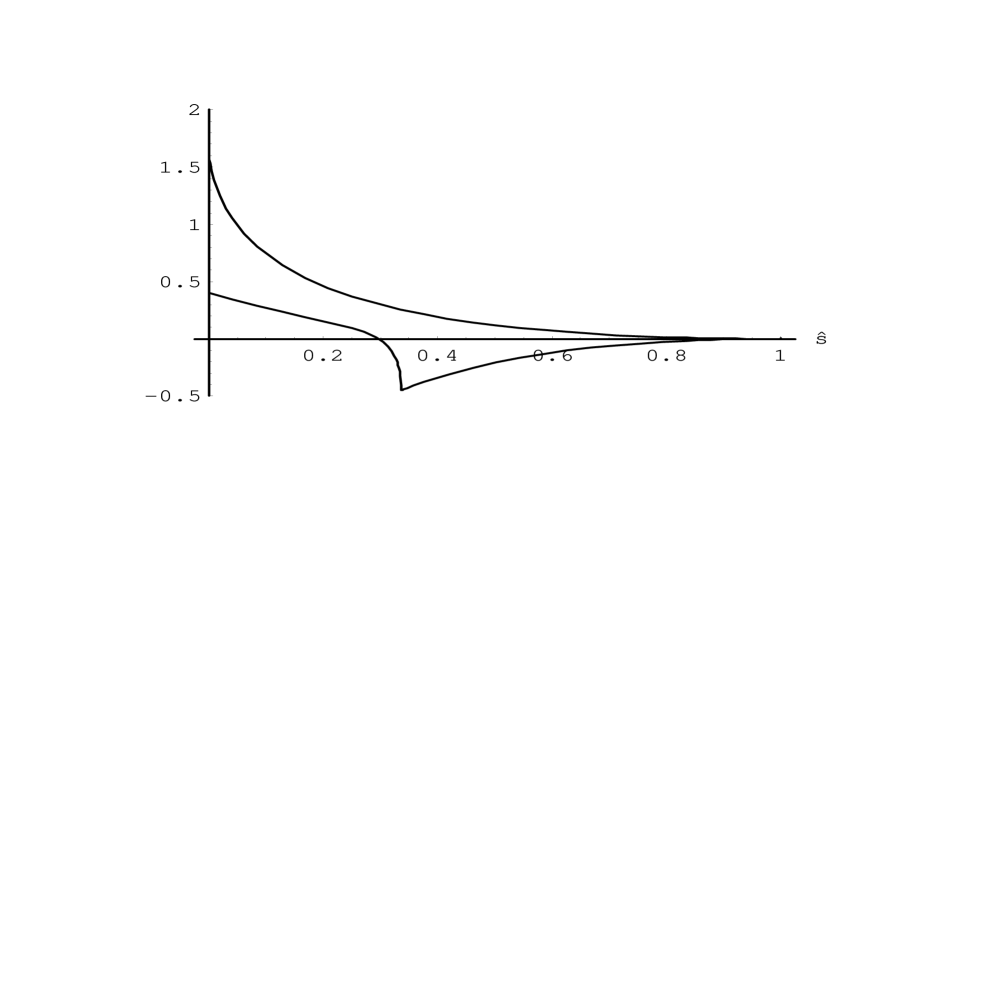
Figure 1: Functions $t_{810}$ (upper curve) and $t_{210}$.

The functions $G_{-1}(t)$ and $G_{0}(t)$ can be found in [16] (Eqn. (30), (31)).
The functions $t_{210}$ and $t_{810}$ are plotted in Fig.1.

4 The details of the calculation and numerical results

As in [19] we will work in the rest frame of the lepton pair. The corresponding formulae have been derived in [19]. For the 3-momenta of b-quark ($\vec{p}_{b}$), $\ell^{+}$ ($\vec{l}_{2}$) and gluon ($\vec{r}$) in that frame of reference we have:

$$\vec{p}_{b}=(|\vec{p}_{b}|,0,0),\,\,\,\vec{l}_{2}=(\frac{\sqrt{s}}{2}cos\theta,\frac{\sqrt{s}}{2}sin\theta,0),$$

$$\vec{r}=(E_{r}cos\theta_{1},E_{r}sin\theta_{1}cos\theta_{2},E_{r}sin\theta_{1}sin\theta_{2}),$$

where

$$cos\theta_{1}=\frac{2E_{b}\sqrt{s}-2E_{r}\sqrt{s}+2E_{r}E_{b}-s-m_{b}^{2}+m_{s}^{2}}{2E_{r}|\vec{p}_{b}|},$$

$E_{b}$ is the energy of the $b$ quark and $E_{r}$ is the energy of gluon. Then the formula for double differential decay width reduces to

$$\frac{d^{2}\Gamma(b\rightarrow sg\ell^{+}\ell^{-})}{d\hat{s}dz}=\frac{m_{b}\hat{s}}{(2\pi)^{6}2^{5}}\times\int\bar{|M|^{2}}(1-{z_{2}}^{2})^{-1/2}dz_{2}dE_{r}dE_{b}$$ (13)

where $\bar{|M|^{2}}$ is the squared matrix element, summed and averaged over spins and colors of the particles in the final and initial states, respectively, $\hat{s}=s/m_{b}^{2}$ and $z=cos\theta$, $z_{2}=cos\theta_{2}$. The boundaries for the integration variables are

$$E^{min}_{r}=\frac{{m_{b}}^{2}+s-2E_{b}\sqrt{s}-{m_{s}}^{2}}{2(E_{b}+|\vec{p_{b}}|-\sqrt{s})}\leq E_{r}\leq\frac{{m_{b}}^{2}+s-2E_{b}\sqrt{s}-{m_{s}}^{2}}{2(E_{b}-|\vec{p_{b}}|-\sqrt{s})}=E^{max}_{r}$$

$$m_{b}\leq E_{b}\leq\frac{m_{b}^{2}+s-m_{s}^{2}}{2\sqrt{s}},\,\ \,\ \,\ -1\leq z_{2}\leq 1$$ (14)

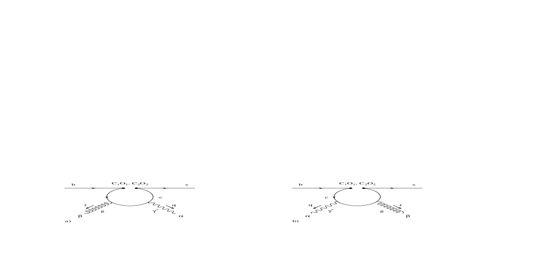
Figure 2: Bremsstrahlung diagrams induced by $O_{1}$ and $O_{2}$.

As we have mentioned above the forward-backward asymmetries arise only from interference of $O_{10}$ matrix element with $O_{i},i=1,..,9$. The infrared infinite bremsstrahlung corrections coming from interference of $O_{10}$ with $O_{7}$ and $O_{9}$ (along with the corresponding virtual corrections) have been taken into account by introducing functions $f_{710}$ and $f_{910}$ which have been calculated in our previous paper. The remaining bremsstrahlung corrections are infrared safe and are coming from the interference of $O_{8}$ and $O_{1}$, $O_{2}$ with $O_{10}$ (see Fig.2 and Fig.3 for the contributing Feinman diagrams).

The calculation of $O_{8}$ and $O_{10}$ interference term is relatively easy and can be performed analytically. The calculation for $O_{1,2}$ and $O_{10}$ interference terms is more complicated and will be described in some detailes below.

The bremsstrahlung corrections involve the matrix elements associated with the two diagrams in Fig. 3. Their sum, $\bar{J}_{\alpha\beta}$, is given by

$$\bar{J}_{\alpha\beta} = \frac{e\,g_{s}\,Q_{u}}{16\,\pi^{2}}\left[E(\alpha,\beta,r)\,\bar{\Delta}i_{5}+E(\alpha,\beta,q)\,\bar{\Delta}i_{6}-E(\beta,r,q)\frac{r_{\alpha}}{qr}\,\bar{\Delta}i_{23}\right.$$ (15)

$$- \left.E(\alpha,r,q)\frac{q_{\beta}}{qr}\,\bar{\Delta}i_{26}-E(\beta,r,q)\frac{q_{\alpha}}{qr}\,\bar{\Delta}i_{27}\right]L\,\frac{\lambda}{2}\,,$$

where $q$ and $r$ denote the momenta of the virtual photon and of the gluon, respectively. The index $\alpha$ will be contracted with the photon propagator, whereas $\beta$ will contracted with the polarization vector $\epsilon^{\beta}(r)$ of the gluon [15]. The matrix $E(\alpha,\beta,r)$ is defined as

$$E(\alpha,\beta,r)=\frac{1}{2}(\gamma_{\alpha}\gamma_{\beta}\hat{r}-\hat{r}\gamma_{\beta}\gamma_{\alpha}).$$ (16)

Due to Ward identities, the quantities $\bar{\Delta}i_{k}$ are not independent of one another. Namely, we have

$$\bar{\Delta}i_{5}=\bar{\Delta}i_{23}+\frac{q^{2}}{qr}\bar{\Delta}i_{27}\,;\quad\bar{\Delta}i_{6}=\bar{\Delta}i_{26}\,.$$ (17)

As in addition $\bar{\Delta}i_{26}=-\bar{\Delta}i_{23}$, the bremsstrahlung matrix elements depend on $\bar{\Delta}i_{23}$ and $\bar{\Delta}i_{27}$, only. In $d=4$ dimensions we find

$$\bar{\Delta}i_{23}=8\,(qr)\int_{0}^{1}\!dx\,dy\,\frac{x\,y(1-y)^{2}}{C}\,,\bar{\Delta}i_{27}=8\,(qr)\int_{0}^{1}\!dx\,dy\,\frac{y\,(1-y)^{2}}{C}\,,$$ (18)

where

$$C=m_{c}^{2}-2\,x\,y(1-y)(qr)-q^{2}\,y\,(1-y)-i\,\delta.$$ (19)

It is easy to notice that dependence of the matrix element $M$ on $z_{2}$ is polynomial so the integral over $z_{2}$ in Eq.(13) is straightforward. To deal with the remaining two dimensional integrals over $\hat{E}_{r}=E_{r}/m_{b}$ and $\hat{E}_{b}=E_{b}/m_{b}$ it is useful to introduce a new integration variable $w$ instead of $\hat{E}_{r}$ defined by $w=2\sqrt{\hat{s}}E_{r}+\hat{s}$ .The integration limits are then given by

$$\hat{E}_{b}\in\left[\frac{\hat{s}+w^{2}}{2w\sqrt{\hat{s}}},\frac{1+\hat{s}}{2\sqrt{\hat{s}}}\right]\quad and\quad w\in[\hat{s},1].$$ (20)

For a fixed value of $\hat{s}$, the quantities $\bar{\Delta}i_{23}$ and $\bar{\Delta}i_{27}$ depend only on the scalar product $qr$, which is given by $(w-\hat{s})\,m_{b}^{2}/2$. The integration over $\hat{E}_{b}$ then turns out to be of rational kind and can be performed analytically. The remaining integration over $w$, however, is more complicated and is done numerically.

We now proceed to the investigation of the numerical impact of the finite bremsstrahlung corrections on the forward-backward asymmetries. In Fig. 4 we show the contribution of the finite bremsstrahlung corrections to the unnormalized forward-backward asymmetry $\Delta A_{FB}(\hat{s})$. Dashed-dot lines show the contribution from interference of matrix elements of the operators $O_{8}$ and $O_{10}$ ($\mu$ =2.5 GeV (uppermost curve), 5 GeV (middle curve), and 10 GeV (lower curve)), dashed lines show the contribution from interference of matrix elements of the operators $O_{1,2}$ and $O_{10}$ ($\mu$ =2.5 GeV (lower curve), 5 GeV (middle curve), and 10 GeV (uppermost curve) and ), solid lines show the sum of previous two terms ($\mu$ =2.5 GeV (lower curve), 5 GeV (middle curve), and 10 GeV (uppermost curve)), $m_{c}/m_{b}$=0.29. We see that contributions coming from $O_{1,2}-O_{10}$ and $O_{8}-O_{10}$ interference terms partially cancel each other. For that reason the contribution of new terms to the forward backward asymmetries is numerically small. In Fig. 5 we combine the new corrections with the previous results for unnormalized forward-backward asymmetry. The solid lines show $A_{FB}(\hat{s})$ including new corrections for three values of renormalization scale ($\mu$=2.5,5 and 10 GeV) and $\hat{m_{c}}=0.29$. The dashed lines represent the corresponding results without finite bremsstrahlung corrections.. In Fig. 6 we give the corresponding curves for normalized forward-backward asymmetry $\bar{A}_{FB}(\hat{s})$. The new contribution is numerically small: at $\hat{s}=0$ we find $A_{FB}^{NNLL}(0)=2.304\pm 0.109$ while without finite bremsstrahlung corrections we have $A_{FB}^{NNLL}(0)=2.292\pm 0.111$. For the position $\hat{s}_{0}$ where forward-backward asymmetry is zero we find $\hat{s}_{0}^{NNLL}=0.1620\pm 0.0016$ while without finite bremsstrahlung corrections we have $\hat{s}_{0}^{NNLL}=0.1615\pm 0.0015$.

It is necessary to mention that for some extensions of the standard model (see for instance, [22]) with opposite sign (and larger values) of $\tilde{C}_{8}^{eff}$ the contribution of the finite bremsstrahlung corrections to the forward-backward asymmetries can be sizable.

To conclude, we have calculated the finite bremsstrahlung corrections to the forward-backward asymmetries for $b\rightarrow X_{s}\ell^{+}\ell^{-}$ decay. We found that the numerical impact of the new corrections on the forward-backward asymmetries in the standard model is less than 1%, but for some extensions of the standard model it can be larger.

ACKNOWLEDGMENTS

We thank C. Greub for useful discussions. The work was partially supported by NFSAT-PH 095-02 (CRDF 12050) and SCOPES programs.

Table 1: Coefficients appearing Eq. (3) for $\mu=2.5$ GeV, $\mu=5$ GeV and $\mu=10$ GeV. For $\alpha_{s}(\mu)$ (in the $\overline{\mbox{MS}}$ scheme) we used the two-loop expression with five flavors and $\alpha_{s}(m_{Z})=0.119$. The entries correspond to the pole top quark mass $m_{t}=174$ GeV. The superscript (0) refers to lowest order quantities.

$\mu$	$2.5$ GeV	$5$ GeV	$10$ GeV
$\alpha_{s}$	$0.2675$	$0.2150$	$0.1800$
$C_{1}^{(0)}$	$-0.6960$	$-0.4860$	$-0.3257$
$C_{2}^{(0)}$	$1.0458$	$1.0235$	$1.0109$
$\raisebox{1.42262pt}{\big{(}}A_{7}^{(0)},~{}A_{7}^{(1)}\raisebox{1.42262pt}{\big{)}}$	$(-0.3605,~{}0.0322)$	$(-0.3207,~{}0.0185)$	$(-0.2873,~{}0.0089)$
$A_{8}^{(0)}$	$-0.1688$	$-0.1535$	$-0.1403$
$\raisebox{1.42262pt}{\big{(}}A_{9}^{(0)},~{}A_{9}^{(1)}\raisebox{1.42262pt}{\big{)}}$	$(4.2407,~{}-0.1700)$	$(4.1283,~{}0.0130)$	$(4.1311,~{}0.1549)$
$\raisebox{1.42262pt}{\big{(}}T_{9}^{(0)},~{}T_{9}^{(1)}\raisebox{1.42262pt}{\big{)}}$	$(0.1148,~{}0.2791)$	$(0.3744,~{}0.2512)$	$(0.5763,~{}0.2307)$
$\raisebox{1.42262pt}{\big{(}}U_{9}^{(0)},~{}U_{9}^{(1)}\raisebox{1.42262pt}{\big{)}}$	$(0.0455,~{}0.0228)$	$(0.0326,~{}0.0153)$	$(0.0224,~{}0.0105)$
$\raisebox{1.42262pt}{\big{(}}W_{9}^{(0)},~{}W_{9}^{(1)}\raisebox{1.42262pt}{\big{)}}$	$(0.0440,~{}0.0162)$	$(0.0321,~{}0.0117)$	$(0.0223,~{}0.0085)$
$\raisebox{1.42262pt}{\big{(}}A_{10}^{(0)},~{}A_{10}^{(1)}\raisebox{1.42262pt}{\big{)}}$	$(-4.3731,~{}0.1349)$	$(-4.3731,~{}0.1349)$	$(-4.3731,~{}0.1349)$

                                           

                                                                                      

Figure 3: Bremsstrahlung diagrams induced by $O_{7}$ and $O_{8}$, $O_{9}$, $O_{10}$.

                                           

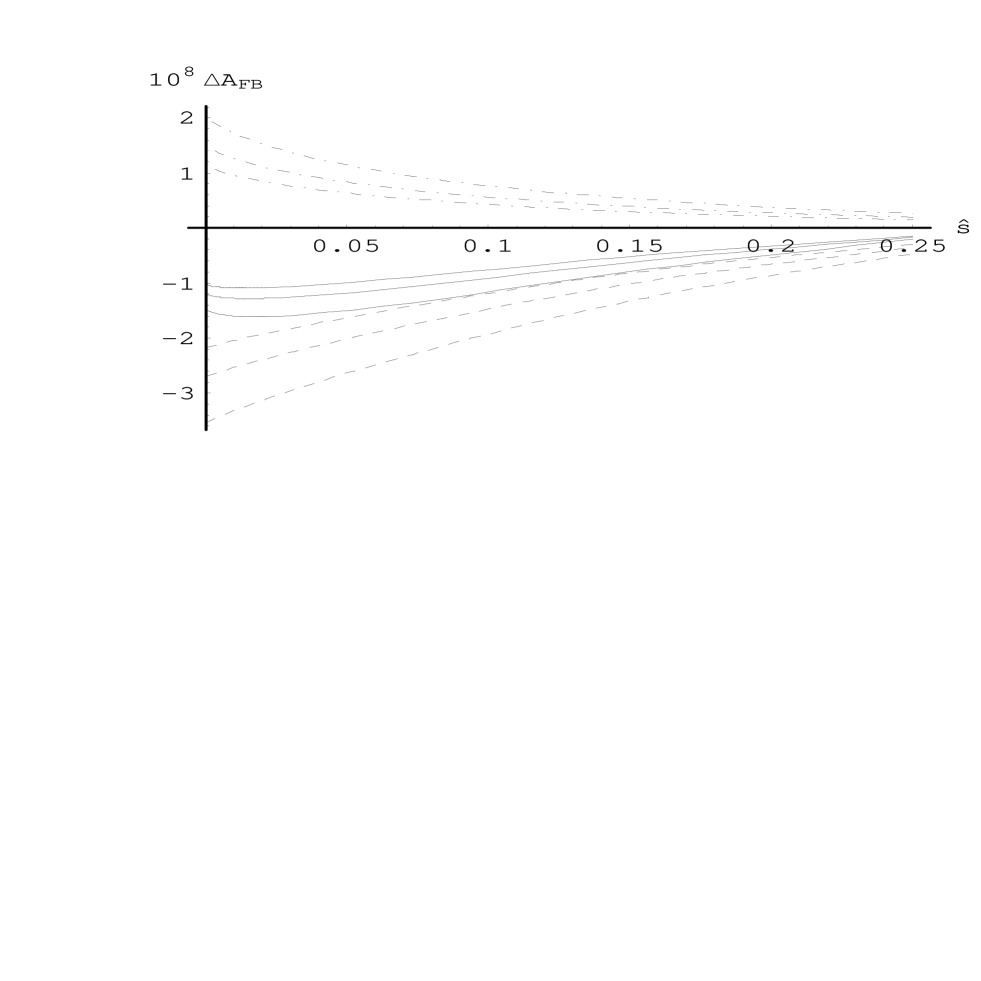
Figure 4: The contribution of finite bremsstrahlung corrections to the unnormalized forward-backward asymmetry. Dashed-dot lines show the contribution from interference of matrix elements of operators $O_{8}$ and $O_{10}$ ($\mu$ =2.5 GeV (uppermost curve), 5 GeV (middle curve), and 10 GeV (lower curve)), dashed lines show the contribution from interference of matrix elements of operators $O_{1,2}$ and $O_{10}$ ($\mu$ =2.5 GeV (lower curve), 5 GeV (middle curve), and 10 GeV (uppermost curve) and ), solid lines show the sum of finite bremsstrahlung contributions ($\mu$ =2.5 GeV (lower curve), 5 GeV (middle curve), and 10 GeV (uppermost curve)), $m_{c}/m_{b}$=0.29.

                                           

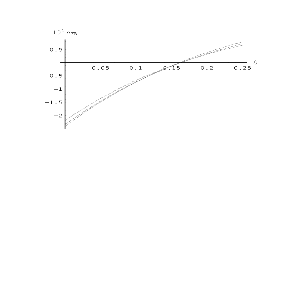
Figure 5: The solid curves show $\hat{s}$ and $\mu$ (for $\mu$=2.5, 5 and 10 GeV) dependence of unnormalized forward-backward asymmetry in NNLL approximation including finite bremsstrahlung corrections while dashed lines show the corresponding results without new corrections.

                                           

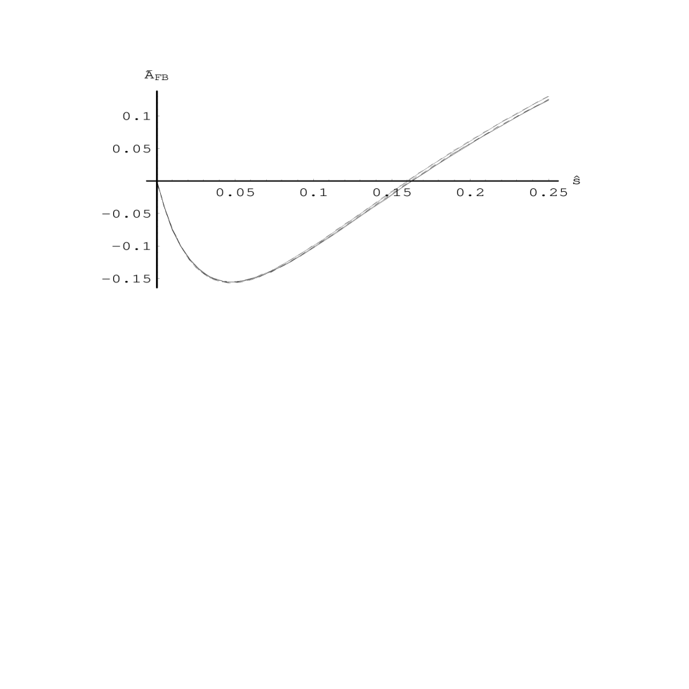
Figure 6: The solid curves show $\hat{s}$ and $\mu$ (for $\mu$=2.5, 5 and 10 GeV) dependence of normalized forward-backward asymmetry in NNLL approximation including finite bremsstrahlung corrections while dashed lines show the corresponding results without new corrections.

References

• [1] K. Abe et al. [BELLE Collaboration], Phys. Rev. Lett. 88, 021801 (2002) [hep-ex/0109026].
• [2] B. Aubert et al. [BABAR Collaboration], hep-ex/0207082.
• [3] J. Kaneko et al. [Belle Collaboration], Phys. Rev. Lett. 90, 021801 (2003) [hep-ex/0208029]
• [4] A. Ali, E. Lunghi, C. Greub, G. Hiller, Phys. Rev. D 66, 034002 (2002) [hep-ph/0112300].
• [5] A. F. Falk, M. Luke and M. J. Savage, Phys. Rev. D 49, 3367 (1994).
• [6] A. Ali, G. Hiller, L. T. Handoko and T. Morozumi, Phys. Rev. D 55, 4105 (1997).
• [7] J-W. Chen, G. Rupak and M. J. Savage, Phys. Lett. B 410, 285 (1997).
• [8] G. Buchalla, G. Isidori and S. J. Rey, Nucl. Phys. B 511, 594 (1998).
• [9] G. Buchalla and G. Isidori, Nucl. Phys. B 525, 333 (1998).
• [10] F. Krüger and L.M. Sehgal, Phys. Lett. B 380, 199 (1996).
• [11] M. Misiak, Nucl. Phys. B393 23 (1993); E:B439 461 1995.
• [12] A. J. Buras and M. Münz, Phys. Rev. D 52, 186 (1995).
• [13] C. Bobeth, M. Misiak and J. Urban, Nucl. Phys. B 574, 291 (2000).
• [14] H. H. Asatrian, H. M. Asatrian, C. Greub and M. Walker, Phys. Lett. B 507, 162 (2001).
• [15] H. H. Asatryan, H. M. Asatrian, C. Greub and M. Walker, Phys. Rev. D 65, 074004 (2002) [arXiv:hep-ph/0109140].
• [16] H. H. Asatryan, H. M. Asatrian, C. Greub and M. Walker, Phys. Rev. D 66, 034009 (2002) [arXiv:hep-ph/0204341].
• [17] T. Goto et al., Phys. Rev. D 55, 4273 (1997); T. Goto et al., Phys. Rev. D 58, 094006 (1998).
• [18] A. Ali, G. Giudice and T. Mannel, Z. Phys. C 67, 417 (1995).
• [19] H. M. Asatrian, K. Bieri, C. Greub and A. Hovhannisyan, Phys. Rev. D 66, 094013 (2002) [arXiv:hep-ph/0209006].
• [20] A. Ghinchulov, T. Hurth, G. Isidori and Y. P. Yao, Nucl. Phys. B 648, 253 (2003) [hep-ph/0208088].
• [21] H. M. Asatrian, H. H. Asatryan, A. Hovhannisyan, V. Poghosyan, in preparation.
• [22] A. L. Kagan, M. Neubert, Phys. Rev. D 58, 094012 (1998).
Refer to caption