ABSTRACT

We present results of an investigation to study CP violation in the Higgs sector in $t\bar{t}$ production at a $\gamma\gamma$-collider, via the process $\mbox{$\gamma\gamma$}\rightarrow\phi\rightarrow t\bar{t}$ where the $\phi$ is a scalar with indeterminate CP parity. The study is performed in a model independent way parametrising the CP violating couplings in terms of six form factors $\{\Re(S_{\gamma}),\Im(S_{\gamma}),\Re(P_{\gamma}),\Im(P_{\gamma}),S_{t},P_{t}\}$. The CP violation is reflected in the polarisation asymmetry of the produced top quark. We use the angular distribution of the decay lepton from $t/\bar{t}$ as a diagnostic of this polarisation asymmetry and hence of the CP mixing, after showing that the asymmetries in the angular distribution are indpendent of any CP violation in the $tbW$ vertex. We construct combined asymmetries in the initial state lepton (photon) polarization and the final state lepton charge and study how well different combinations of these form factors can be probed by measurements of these asymmetries, using circularly polarized photons. We demonstrate the feasibility of the method to probe CP violation in the Higgs sector at the level induced by loop effects in supersymmetric theories, using realistic photon spectra expected for a TESLA like $e^{+}e^{-}$ collider. We investigate the sensitivity of our method for for different widths of the scalar as well as for the more realistic backscattered laser photon spectrum resulting from the inlcusion of the nonlinear effects.

1 Introduction

While the standard model (SM) has been proved to provide the correct description of all the fundamental particles and their interactions, direct experimental verification of the Higgs sector and a basic understanding of the mechanism for the generation of the observed CP violation is still lacking. Many models with an extended Higgs sector have CP violation in the Higgs sector. In this context there are then two important questions that need to be answered viz., if CP is conserved in the Higgs sector, how well can the CP transformation properties of the, possibly more than one, neutral Higgses be established. If it is violated then one wishes to study how is this CP violation reflected in Higgs mixing as well as couplings and how well can these be measured at the colliders. CP violation in the Higgs sector can be either explicit, spontaneous or loop-induced. The last has been studied in great detail in the context of the minimal Supersymmetric Standard Model (MSSM) recently [1] and arises from loops containing sparticles and nonzero phases of the MSSM parameters $\mu$ and $A_{t}$.

$\gamma\gamma$ colliders will make possible an accurate measurement of the width of a Higgs scalar into $\gamma\gamma$ [2] and $WW/ZZ$ [3] channels. A study of the former can give very important information about the physics beyond standard model (SM) due to the nondecoupling nature of this width. Further, $\gamma\gamma$ collisions will also offer the possibility of a study of heavy neutral Higgses $H/A$ of the MSSM through their production in $\gamma\gamma$ collisions, followed by their decay into a pair of neutralinos, thus making possible an exploration of the MSSM Higgs sector in a region of the parameter space not accessible to the LHC [4].

Photon Colliders with their democratic coupling to both the CP even and the CP odd scalars and the possibility of polarised photon beams, offer the best chance to explore the CP property of the scalar sector. Using $\gamma\gamma$ colliders with linearly polarised photon beams, it is possible to study the CP property of the Higgs from just the polarisation dependence of the cross-section [5]. The $ZZ$ decay can also be used very effectively to make a model independent determination of the CP nature of the Higgs boson at the $e^{+}e^{-}$, $\gamma\gamma$ colliders as well as the LHC/citedavid. It has been shown [7] that even in the case of photon colliders with just the circular polarisation, it might be possible to probe the CP property of the Higgs by looking at the net polarisation of the top quarks produced in the process $\gamma\gamma\rightarrow\phi\rightarrow t\bar{t}$. With linearly polarised $\gamma$ and the $t\bar{t}$ decay of the scalar it should be possible to completely reconstruct the $\phi\gamma\gamma$ and the $\phi t\bar{t}$ vertex, using the resulting polarisation asymmetries of the $t$. The $t$ quark being very heavy decays before it hadronises. Hence the decay lepton energy and angular distributions can be used as an analyser of the $t$ polarisation [8]. Thus a study of the simple inclusive lepton angular distributions in the $\gamma\gamma\rightarrow\phi\rightarrow t\bar{t}$. can yield information about the CP property of the $\phi$. We considered $\gamma\gamma$ production of a $t\bar{t}$ pair through the s-channel exchange of a scalar $\phi$ of indeterminate CP property and studied [9] how well the CP property of such a scalar can be probed using mixed asymmetries with respect to the final state lepton charge and initial state photon polarisation. Our analysis considered only the case of circularly polarised lasers. Recently, a calculation [10] of helicity amplitudes for the consequent lepton production coming from the $t$ decay has been performed including the case of the linear polarisation of the laser photon.

In sections 2 and 3, I recapitulate the notation, the methodology, along with a discussion of the independence of the decay lepton angular distribution from any anomalous $tbW$ vertex. I end with an example of the sensitivity expected for a particular point in the MSSM parameter space at a $\gamma\gamma$ collider with ideal backscattered laser photon spectrum[11]. In the last section, I then present update of these results using the parametrisation [12] of a more realistic backscattered laser spectrum resulting from inclusion of nonlinear effects [13] and that of a variation in the width of the scalar.

2 Formalism and calculation of the decay $l$ angular distribution

The process we study is shown in Fig. 1.

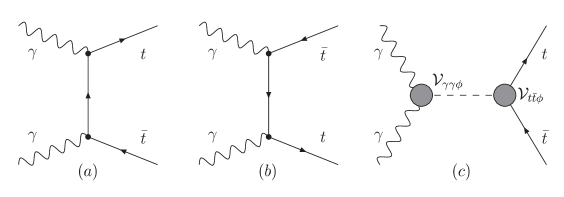
Figure 1: Feynman diagrams for the $t\bar{t}$ production in $\gamma\gamma$ collisions.

The diagrams shown in Figs. 1 (a) and 1 (b) give what we will deonote later as the SM contirbution and Fig. 1 (c) shows the contribution from the production of a scalar $\phi$ with indeterminate CP parity. The most general model independent expression for the $\phi\gamma\gamma$ and $\phi t\bar{t}$ vertices for such a $\phi$ that we use is written as,

$${\cal V}_{t\bar{t}\phi}=-ie\frac{m_{t}}{M_{W}}\left(S_{t}+i\gamma^{5}P_{t}\right),$$ (1)

$${\cal V}_{\gamma\gamma\phi}=\frac{-i\sqrt{s}\alpha}{4\pi}\left[S_{\gamma}(s)\left(\epsilon_{1}.\epsilon_{2}-{2\over s}(\epsilon_{1}.k_{2})(\epsilon_{2}.k_{1})\right)\right.-\left.{2P_{\gamma}(s)\over s}\epsilon_{\mu\nu\alpha\beta}\epsilon_{1}^{\mu}\epsilon_{2}^{\nu}k_{1}^{\alpha}k_{2}^{\beta}\right].$$ (2)

Here $k_{1}$ and $k_{2}$ are the four-momenta of colliding photons and $\epsilon_{1,2}$ are the photon polarisation vectors. Form factors $S_{t},P_{t}$ can be taken to be real without any loss of generality whereas the most general $S_{\gamma},P_{\gamma}$ are required to be complex. Simultaneous presence of nonzero $P,S$ coupling implies CP violation. Of course in a given model the predictions for $P_{t},S_{t}$ and $P_{\gamma},S_{\gamma}$ are correlated. The most general $tbW$ vertex can be written as,

$$\Gamma^{\mu}_{tbW} =-\frac{g}{\sqrt{2}}V_{tb}\left[\gamma^{\mu}\left(f_{1L}P_{L}+f_{1R}P_{R}\right)\right.-\left.\frac{i}{M_{W}}\sigma^{\mu\nu}(p_{t}-p_{b})_{\nu}\left(f_{2L}P_{L}+f_{2R}P_{R}\right)\right]$$ (3)

$${\bar{\Gamma}}^{\mu}_{tbW} =-\frac{g}{\sqrt{2}}V_{tb}^{*}\left[\gamma^{\mu}\left({\bar{f}}_{1L}P_{L}+{\bar{f}}_{1R}P_{R}\right)\right.-\left.\frac{i}{M_{W}}\sigma^{\mu\nu}(p_{\bar{t}}-p_{\bar{b}})_{\nu}\left({\bar{f}}_{2L}P_{L}+{\bar{f}}_{2R}P_{R}\right)\right]$$ (4)

Following LEP measurements we take $f_{1L}={\bar{f}}_{1L}=1$. All the other $f_{i},\bar{f}_{i}$ are necessarily small. $f_{2R},{\bar{f}}_{2L}$ are the only nonstandard part of the $tbW$ vertex that contribute to the angular and energy distribution of the lepton in the limit $m_{b}=0$. In our analysis we keep only terms linear in them. We calculate the analytical expression for helicity amplitudes and the differential cross-section for $\gamma\gamma\rightarrow t\bar{t}\rightarrow l^{+}b\nu_{l}\bar{t}$ and the angular distribution of the consequent decay lepton using the general $\phi t\bar{t},\phi\gamma\gamma$ and the $tbW$ vertices given above.

Independence of the $l$ angular distribution from the anomalous part of the $tbW$ vertex.

The expression for the differential distribution for the decay lepton $l$ can be written as

$$\frac{d\sigma}{d\cos\theta_{t}\ d\cos\theta_{l^{+}}\ dE_{l^{+}}\ d\phi_{l^{+}}}=\frac{3e^{4}g^{4}\beta E_{l^{+}}}{64(4\pi)^{4}s\Gamma_{t}m_{t}\Gamma_{W}M_{W}}\sum_{\lambda,\lambda^{\prime}}\underbrace{\rho^{\prime+}(\lambda,\lambda^{\prime})}_{c.m.\ frame}\underbrace{\left[\frac{\Gamma^{\prime}(\lambda,\lambda^{\prime})}{m_{t}E_{l^{+}}^{0}}\right]}_{rest\ frame}.$$ (5)

In the above, $E_{l^{+}}^{0}$ is energy of $l^{+}$ in the rest frame of $t$ quark. The production and decay density matrices $\rho^{+}(\lambda,\lambda^{\prime}),\Gamma(\lambda,\lambda^{\prime})$ are given by

$$\rho^{+}(\lambda,\lambda^{\prime})=e^{4}\rho^{\prime+}(\lambda,\lambda^{\prime})=\sum\rho_{1}(\lambda_{1},\lambda_{1}^{\prime})\rho_{2}(\lambda_{2},\lambda_{2}^{\prime}){\cal M}(\lambda_{1},\lambda_{2},\lambda,\lambda_{\bar{t}}){\cal M}^{*}(\lambda_{1}^{\prime},\lambda_{2}^{\prime},\lambda^{\prime},\lambda_{\bar{t}})$$ (6)

$$\Gamma(\lambda,\lambda^{\prime})=g^{4}|\Delta(p_{W}^{2})|^{2}\ \Gamma^{\prime}(\lambda,\lambda^{\prime})=\frac{1}{2\pi}\int d\alpha\times\sum M_{\Gamma}(\lambda,\lambda_{b},\lambda_{l^{+}},\lambda_{\nu})\ M_{\Gamma}^{*}(\lambda^{\prime},\lambda_{b},\lambda_{l^{+}},\lambda_{\nu})$$ (7)

In the above, $\alpha$ is the azimuthal angle of $b$-quark in the rest-frame of $t$-quark with $z$-axis pointing in the direction of momentum of lepton and $\rho_{1(2)}$ are the photon density matrices. The decay density matrix elements are in the $t,\bar{t}$ frame. For example the $+,+(-,-)$ element is given by,

$$\Gamma(\pm,\pm)=g^{4}m_{t}E_{l^{+}}^{0}|\Delta_{W}(p_{W}^{2})|^{2}\ (m_{t}^{2}-2p_{t}.p_{l^{+}})(1\pm\cos\theta_{l^{+}})\left(1+\frac{\Re(f_{2R})}{\sqrt{r}}\frac{M_{W}^{2}}{p_{t}.p_{l^{+}}}\right)$$ (8)

The decay $l$ angular distribution can be obtained analytically by integrating Eq. 5 over $E_{l},\cos\theta_{t}$ and $\phi_{l}$. We find that the only effect of the anomalous part of the $tbW$ coupling on $l$ angular distribution is an overall factor $1+2r-6\Re(f^{\pm})\sqrt{r}$ independent of any kinematical variables. We further find that the total width of $t$-quark calculated upto linear order in the anomalous vertex factors receives the same factor. As a result the angular distribution of the decay lepton is unaltered by the anomalous part of the $tbW$ couplings to the linear approximation. Since the correlation between the top spin and the angle of emission of the decay lepton is essentially a result of the $V-A$ nature of the $tbW$ coupling, it can be thus used as a true polariometer for the polarisation of the $t$. The energy distribution of the decay lepton, which also reflects the polarisation of the parent $t$ quark does get affected by the presence of the anomalous part of the $tbW$ couplings. Thus the angular distribution of the decay $l$ is a very interesting observable for which the only source of the CP violating asymmetry will then be the production process. Further, the construction of CP violating asymmetries using the angular distributions of the decay $l$ does not need precise reconstruction of the top rest frame and the consequent prescise knolwedge of the top quark momentum. For the case of $e^{+}e^{-}\rightarrow t\bar{t}$ followed by subsequent $t/\bar{t}$ decay, this was observed earlier [14, 15]. It was proved recently by two groups independently; for a two-photon initial state by Ohkuma [16], for an arbitrary two-body initial state in [17] and further keeping $m_{b}$ non-zero in [18]. These latter derivations use the method developed by Tsai and collaborators [19] for incorporating the production and decay of a massive spin-half particle. Our current derivation made use of helicity amplitudes and provides an independent verification of these results.

3 Asymmetries and their sensitivity to CP violation expected due to loop effects

The cross-section has a nontrivial dependence on the poalrisation of the initial state photons as $\phi$ exchange diagram contributes only when both colliding photons have same helicity due to its spin $0$ nature. Further, SM contribution is peaked in the forward and backward direction whereas the scalar exchange contribution is independent of the production angle $\theta_{t}$. Hence angular cuts to redcue the SM contribution along with choice of equal helicities for both the colliding photons can maximise polarisation asymmetries for the produced $t\bar{t}$ pair, giving a better measure of the $CP$ violating nature of the $s-$ channel contribution. Another thing to note is that the polarisation of the collidiing photon is decided by the polarisation of the initial lepton and that of the laser photon used in the backscattering which gives rise to the energetic colliding photon.

Figure 2: Energy spectrum and the polarisation expected for the backscattered laser for ideal case  [11]

Fig. 2 shows the energy spectrum and the polarisation expected for the backscattered laser for the ideal case  [11], i.e., neglecting the nonlinear effects, for different choices of the $e$ and the laser polarisation. One can choose $\lambda_{e}\lambda_{l}=-1$ to get a hard photon spectrum. Further, as discussed above, one sets $\lambda_{e^{-}}=\lambda_{e^{+}}$ to maximise the sensitivity to possible $CP$ violating interactions coming from the scalar exchange. Thus all the polarisations are fixed wrt to that of one of the leptons. Thus there are two choices of the initial state lepton polarisation, $\lambda_{e^{-}}=\lambda_{e^{+}}=+1$ and $-1$. In the final state one can look for either $l^{+}$ or $l^{-}$. This makes four possible combination of cross-sections depending on the initial state photon and the final state $l$ charge: $\sigma(+,+),\sigma(+,-),\sigma(-,+)$ and $\sigma(-,-)$. CP conservation will imply, for example for the QED contribution which we call the SM contribution, $\sigma(+,+)=\sigma(-,-)$. Using these now we construct asymmetries which will be sensitive to $\phi$ coupling.

Asymmetries

For defining asymmetries, we choose two polarised cross-section at a time out of four available, and can define six asymmetries as,

$${\cal A}_{1}=\frac{\sigma(+,+)-\sigma(-,-)}{\sigma(+,+)+\sigma(-,-)};{\cal A}_{2}=\frac{\sigma(+,-)-\sigma(-,+)}{\sigma(+,-)+\sigma(-,+)};{\cal A}_{3}=\frac{\sigma(+,+)-\sigma(-,+)}{\sigma(+,+)+\sigma(-,+)}$$

$${\cal A}_{4}=\frac{\sigma(+,-)-\sigma(-,-)}{\sigma(+,-)+\sigma(-,-)};{\cal A}_{5}=\frac{\sigma(+,+)-\sigma(+,-)}{\sigma(+,+)+\sigma(+,-)};{\cal A}_{6}=\frac{\sigma(-,+)-\sigma(-,-)}{\sigma(-,+)+\sigma(-,-)}$$ (9)

${\cal A}_{5}$ and ${\cal A}_{6}$ are charge asymmetries for a given polarisation. These will be zero if $\theta_{0}\rightarrow 0$. The same is not true of course of the purely CP violating ${\cal A}_{1}$ and ${\cal A}_{2}$. ${\cal A}_{3}$ and ${\cal A}_{4}$ are the polarisation asymmetries for a given lepton charge. The phenomenon of nonvanishing charge asymmetries even for the SM case, for polarised photon beams has been also been observed recently in the context of $\mu+\mu-$ pair production[20]. However these can not be directly compared as we have constructed the asymmetries in terms of the polarisation of the incoming lepton beam rather than that of the photon. The contribution of the $s$ channel diagram to the asymmetries can be enhanced by the choice of relative polarisation of the $e^{+}e^{-}$ beams and the angular cuts as mentioned above as well as that of the beam energy. Of course only three of the asymmetries given above are linearly independent of each other. The sensitivity of the these asymmetries to the various couplings of the scalar $\phi$ in general and to the CP violating part in particular, can be best judged by taking a specific numerical example.

To that end we choose the values of the form factors obtained in the second of Ref. [7] for $\tan\beta=3$, with all sparticles heavy and maximal phase: $m_{\phi}=500GeV,\Gamma_{\phi}=1.9GeV,S_{t}=0.33,P_{t}=0.15,S_{\gamma}=-1.3-1.2i,P_{\gamma}=-0.51+1.1i.$

Figure 3: Asymmetries expected for the SM cotribution (continuum) and for the chosen MSSM point (solid line)

We notice that the expected asymmetries are not insubstantial. Even the CP violating asymmetries are at the level of $3$–$4$ %. The results presented correspond to a cut on the lepton angle $\theta_{0}=60^{\circ}$. The choice of the cutoff angle on the lepton and also of the energy was optimised by studying the sensitivity of a particular asymmetry measurement. The number of events corresponding to the asymmetry are ${\cal L}\Delta\sigma$. For the asymmetry to be measurable say at $95\%$ CL, we must have at least ${\cal L}\Delta\sigma>1.96\sqrt{{\cal L}\sigma}$. A measure of the senstivity thus can be

$${{{\cal L}{\Delta\sigma}}\over{1.96\sqrt{{\cal L}\sigma}}}={\sqrt{{\cal L}}\over 1.96}\times{{\Delta\sigma}\over{\sqrt{\sigma}}}$$

The larger the asymmetry as compared to the fluctuations, the larger the sensitivity with which it can be measured. We define sensitivity as, ${\cal S}=\frac{{\cal A}}{\delta{\cal A}}\propto\frac{\Delta\sigma}{\sqrt{\sigma}}$. For this choice of the scalar mass and the ideal backscattered photon, the cross-sections, the asymmetries and the sensitivity is optimised by choosing $E_{b}=310$ GeV and two choices of angular cuts $20^{\circ}$ and $60^{\circ}$. With this choice of energy and the ideal Ginzburg spectrum, we then anlaysed how well various scalar couplings can be studied using these asymmetries.

Analysis of the sensitivity of these asymmetries to the scalar couplings:

$CP$ properties of the Higgs determined if we know all the four form-factors $S_{t},P_{t},$ $\Re(S_{\gamma}),\Im(S_{\gamma}),$ and $\Re(P_{\gamma}),\Im(P_{\gamma})$. They appear in the production density matrix in eight combinations, $x_{i}$ and $y_{i}$, $(i=1,...4)$ given by;

$$x_{1}=S_{t}\Re(S_{\gamma}),\ x_{2}=S_{t}\Im(S_{\gamma}),\ x_{3}=P_{t}\Re(P_{\gamma}),\ x_{4}=P_{t}\Im(P_{\gamma})$$ (10)

$$y_{1}=S_{t}\Re(P_{\gamma}),\ y_{2}=S_{t}\Im(P_{\gamma}),\ y_{3}=P_{t}\Re(S_{\gamma}),\ y_{4}=P_{t}\Im(S_{\gamma}).$$ (11)

$x_{i}$ given by Eq.  10 all being CP even and $y_{i}$ of Eq.  11 all CP odd. Only five of these are linearly independent and we have,

$$y_{1}.y_{3}=x_{1}.x_{3},\ y_{2}.y_{4}=x_{2}.x_{4},\ y_{1}.x_{4}=y_{2}.x_{3},y_{4}.x_{1}=y_{3}.x_{2}.$$ (12)

Since all the asymmetries are functions of $x_{i},y_{i},i=1,4$ one would like to explore the sensitivity of the asymmetry measurements to values of $x_{i},y_{i}$. If for certain values of the form-factors the asymmetries lie within the fluctuation from their SM values, then that particlar point in the parameter space cannot be distinguished from SM at that luminosity. Using this as the criterion we can identify regions in the $x_{i}$–$y_{j}$ plane where it is possible to probe a particular non-zero value of $x_{i},y_{j}$ and hence probe the deviation from the SM amplitude. The region where this is not possible can be termed as the blind region of the particular asymmetry being considered. Thus the set of parameters {$x_{i},y_{i}$} will be inside the blind region at a given luminosity if,

$$|{\cal A}(\{x_{i},y_{i}\})-{\cal A}_{SM}|\leq\delta{\cal A}_{SM}=\frac{f}{\sqrt{\sigma_{SM}L}}\sqrt{1+{\cal A}_{SM}^{2}}.$$

It is clear that using just the three linearly independent asymmetries it will not be possible to extract all the $x_{i},y_{i}$ and hence all the form factors involved, Instead we take only two of the eight $x_{i},y_{j}$ nonzero at a time and ask how well one can constrain these using the measurements of the asymmetries at a given luminosity. We study blind regions in the various $x_{i}$–$y_{j}$ planes for all the different asymmetries and choose the best one in each case. The analysis is performed for the choice of the beam energy $E_{b}$ and angular cut $\theta_{0}$ mentioned above.

Figure 4: Blind regions in the various $x_{i}$–$y_{j}$ planes, the larger and smaller region corresponding to luminosity $500{\rm fb}^{-1}$, $1000{\rm fb}^{-1}$ respectively.

Fig. 4 shows the blind regions in the various $x_{i}$–$y_{j}$ planes; the larger and smaller region corresponding to a luminosity of $500{\rm fb}^{-1},$ and $1000{\rm fb}^{-1}$ respectively. Thus we see that these asymmetries do indeed have the potential of probing nonzero values of $y_{i}$ and hence probing the CP violation in the Higgs sector.

	min	max	min	max	MSSM
	(500 fb-1)	(500 fb-1)	(1000 fb-1)	(1000 fb-1)	value
$x_{1}$	$-3.775$	3.594	$-2.990$	2.869	$-0.429$
$x_{2}$	$-3.413$	3.896	$-2.748$	3.111	$-0.396$
$x_{3}$	$-2.386$	2.873	$-1.842$	2.386	$-0.077$
$x_{4}$	$-2.837$	2.465	$-2.375$	1.930	$+0.165$
$y_{1}$	$-2.786$	2.786	$-2.148$	2.148	$-0.168$
$y_{2}$	$-3.095$	3.095	$-2.433$	2.433	$+0.363$
$y_{3}$	$-2.155$	2.155	$-1.687$	1.687	$-0.195$
$y_{4}$	$-2.346$	2.346	$-1.867$	1.867	$-0.180$

Table 1: Limits possible on $x_{i},y_{j}$ for two different luminosities at $95\%$ CL

The results of Fig. 4 can also be summarised in terms of limits upto which the $x_{i},y_{j}$ can be probed using the measurements of asymmetries alone, if all of them are allowed to vary simultaneously. These are given in Table 1. The last column gives values expected for the chosen MSSM point. It is clear that the limits that the asymmetries can put if all of the $x_{i},y_{j}$ are allowed to vary simultaneously are not very good. But two things should be noted here. Firstly one is sugeesting this as a second generation experiment after the Higgs discovery, hence one might be able to use the known partial information on $x_{i},y_{j}$ and thus be able to constrain these combinations and hence the form factors better. Secondly, it has been shown that with the use of linearly polarised photons one can indeed reconstruct all the form factors completely [7, 10]. It would be interesting to extend our analysis to the case of the linearly polarised photons as well.

Discrimination between the SM and the MSSM

We also investigated the confidence level with which the particular MSSM point chosen by us can be discriminiated from the QED SM background using the asymmetries alone. To that end we calculated the $x_{i},y_{j}$ for our choice of CP violating parameters given by the MSSM point and then investigated the geometry of the blind regions about this point. Again we varied a pair of $x_{i},y_{j}$ at a time, keeping all the other fixed at the values expected for the MSSM point. We thus obtained the blind regions around the point the same way as we did for the SM.

Figure 5: Blind regions for the chosen MSSM point and that for the plain SM QED contribution for $1000{\rm fb}^{-1}$ at $95\%$ CL.

Fig.  5 shows that the blind regions for the SM point and around the MSSM point have very little overlap. This demonstrates that the method is indeed sensitive to the CP violation at the level produced by loop effects.

4 Effect of higher Higgs width and more realistic photon spectra

It is obvious that the sensitivity will depend critically on the width of the scalar and is likely to decrease as the width increases. Further, the energy spectrum of the backscattered laser photon and more importantly the polarisation is subject to large effects from multiple interactions.

Figure 6: The energy spectrum for the single photon and the spectrum in the two photon invariant mass $W_{\gamma\gamma}$ for the backscattered laser photons after inclusion of the nonlinear effects as parametrised in [12] and compared with simulation [13], for $E_{beam}=250$ GeV.

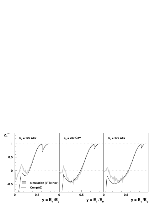
Figure 7: The polarisation $P_{\gamma}$ for the backscattered laser photon as a function of the fraction of the beam energy carried by the photon, after inclusion of the nonlinear effects as parametrised in [12] and compared with simulation [13], for $E_{beam}=100,250$ and $400$ GeV.

The latter is illustrated in Figs. 6, 7 taken from Ref. [12]. Fig. 6 shows the The energy spectrum for the single photon and the spectrum in the two photon invariant mass $W_{\gamma\gamma}$ for the backscattered laser photons after inclusion of the nonlinear effects, as parametrised in [12] and compared with simulation [13], for $E_{beam}=250$ GeV. Fig. 7 shows the expected polarisation for three different values of the beam energy. This is to be compared with right panel of Fig. 2. Since the asymmetries depend crucially on the polarisation it is likely that our study of sensitivity will get affected by this change in the spectrum and the polarisation. Further, for this more realistic case the $e^{-}$ is taken to have only $85\%$ polarisation as opposed to the $100\%$ assumed in our earlier study. Fig.8 shows four of the asymmetries of Eq. 9 obtained using the CompAZ parametrisation [12] of the more realistic spectra [13], plotted as a function of $E_{b}$ .

Figure 8: Four of the asymmetries of Eq. 9 for the ideal and for the realistic spectrum.

For the more realistic spectrum there is also a net decrease in the effective luminosity as the multiple interactions increase the number of the photons in the low energy region. The major effect of the use of the more realistic spectrum seems to be this decrease in the luminosity of the useful, energetic photons.

Even though we have performed our studies in a model independent way, we are specifically also interested in the case of a MSSM scalar. The heavy MSSM scalar is not expected to be very wide.

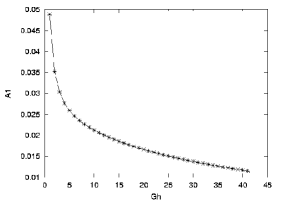
Figure 9: Asymmetry ${\cal A}_{1}$ as a function of the width of the scalar $\Gamma_{\phi}$ in GeV.

Fig. 9 shows the effect on the asymmetry ${\cal A}_{1}$ of changing the width. Thus it is clear that the asymmetries and hence the sensitivities will decrease with increasing width. This is borne out by a study of the blind regions in the various $x_{i}$–$y_{j}$ planes analogous to our earlier anaylsis, for different values of the widths of the scalar.

Next we also study the maximum width of the scalar upto which we can discriminate between the SM and the MSSM point at $95\%$ C.L. To that end we emply the following procedure. It is clear that the SM and the model point chosen will not be confused with each other if the value of the asymmetry expected for the SM and that for the model point chosen do not overlap at $95$ C.L. We generate normally distributed random numbers centered at the asymmetry corresponding to the SM and take 1 $\sigma$ fluctuation of the SM asymmetry as the standard deviation. Let $N_{0}$ number of generated points. Let $N_{1}$ denote the number of points for which the asymmetry value lies within fluctuation expected at $95\%$ C.L. for the expectation of the chosen point. Now probability ${\cal P}$ of confusing SM with this point at $95\%$ is given by $N_{1}/N_{0}$. Probability $P_{0}$ that $95\%$ C.L. intervals of the SM and example point just touch is of course 0.025. In this case if we define

$$S_{1}=1-\frac{{\cal P}}{{\cal P}_{0}},$$

it is easy to see that for $1>S_{1}>0$ the $95\%$ C.L. intervals of the SM asymmetry and that expected at the example point do not overlap. Thus for this case a clear discrimination between the example point and the SM possible. $S<0$ implies that no such discrimination is possible. $S_{1}$ can thus be used quite effectively as a measure of possible discrimination. Of course, ${\cal P}$ is dependent on the angular cut as well as the chosen chosen. We choose the one that gives the smallest $\cal P$ and then plot $S_{1}$ for different ${\Gamma_{\phi}}$ and ${\cal L}$. This is shown in Fig. 10. The choice of the beam energy and the cut off angles are the same as used in the earlier analysis.

Figure 10: $S_{1}$ as a function of width of the scalar $\Gamma_{\phi}$ for different luminosities for the chosen MSSM point and the ideal backscattered photon spectrum.

The figure shows that for a luminosity of 600 fb^-1 we can distinguish SM and the chosen MSSM point, with high sensitivity upto $\Gamma_{\phi}=14$ GeV. Note that this compares well with maximum width expected for a heavy MSSM scalar.

In view of the rather large effects on the asymmetries and the luminosities of using the more realistic spectra it is necessary to make a similar study in that case as well, after optimising the choice of energy and the cutoff angle $\theta_{0}$.

5 Conclusions

Thus to summarise, we have Studied $\gamma\gamma\rightarrow\phi\rightarrow t\bar{t}$; $\phi$ being a scalar with indefinite CP parity. We looked at the process $\gamma\gamma\rightarrow t\bar{t}\rightarrow l^{\pm}X$, where the $l^{+}/l^{-}$ comes from decay of $t/\bar{t}$. We used the most general, CP nonconserving ${\cal V}_{\phi\gamma\gamma},{\cal V}_{t\bar{t}\phi}$ vertices. CP violation in these vertices can give rise to net polarisation asymmetry for the $t$. We used the angular distribution for the decay $l$ coming from the $t$ as an analyser of $t$ polarisation and hence of CP violation in the Higgs sector. We performed our studies in a model independent way by parametrizing the ${\cal V}_{\phi\gamma\gamma},{\cal V}_{t\bar{t}\phi}$ vertices in terms of form factors. We showed that decay lepton angular distribution is insensitive to any anomalous part of the $tbW$ coupling $f^{\pm}$ to first order. As a result it can be a faithful analyser of the CP violation of the production process. We constructed combined asymmetries involving the initial lepton (and hence the laser photon) polarisation and the decay lepton charge. We showed that these can put limits on $CP$ violating combinations, of the form factors, $y$’s, when only two combinations are varied at a time. By taking an example MSSM point. We showed that indeed the constructed asymmetries have sensitivity to CP violation exepected at loop level in the Higgs sector of the MSSM. We further studied the effect of taking a more realistic spectrum for the backscattered laser photon including the nonlinear effects as well as the effect of an increase in the width of the scalar. We developed a measure $S_{1}$ to gauge the ability of the asymmetries to discriminate between the SM and our chosen MSSM point, if the scalar were to have larger width, keeping all the other form factors the same. We were able to show that with a luminosity of 600 fb^-1 we can discriminate between the SM and the chosen MSSM point with high sensitivity upto $\Gamma_{\phi}=14$ GeV.

Acknowledgements
It is a pleasure to thank T. Matsui, Y.Fujii and R. Yahata for the impeccable organisation of the conference in this beautiful place, which provided a wonderful backdrop for the very nice/useful discussions that took place. I would like to acknowledge financial support of JSPS which made the participation possible. Thanks are also due to the DESY Theory group for the hospitality where part of this work was carried out. The work was partially supported by the Department of Science and Technology, India, under project no. SP/S2/K-01/2000-II.

References

- [1] A. Pilaftsis and C. E. M. Wagner, Nucl. Phys. B553 (1999) 3 (hep-ph/9902371); S. Y. Choi, M. Drees and J. S. Lee, Phys. Lett. B481 (2000) 57; M. Carena, J. Ellis, A. Pilaftsis and C. E. M Wagner, Nucl. Phys. B586 (2000) 92 (hep-ph/0003180), S.Y. Choi and J.S. Lee, Phys. Rev. D62 (2000) 036005 (hep-ph/9912330).
- [2] G. Jikia and S. Soldner-Rembold, Nucl. Instrum. Meth. A 472 (2001) 133 (hep-ex/0101056).
- [3] P. Niezurawski, A.F. Zarnecki and M. Krawczyk, hep-ph/0207294. S. Y. Choi, D. J. Miller, M. M. Muhlleitner and P. M. Zerwas, hep-ph/0210077.
- [4] M. M. Muhlleitner, M. Kramer, M. Spira and P. M. Zerwas, Phys. Lett. B 508 (2001) 311 (hep-ph/0101083).
- [5] B. Grzadkowski and J. F. Gunion, Phys. Lett. B 294 (1992) 361–368.
- [6] S. Y. Choi, D. J. Miller, M. M. Muhlleitner and P. M. Zerwas, Phys. Lett. B 553 (2003) 61 (hep-ph/0210077).
- [7] E. Asakawa, J.-i. Kamoshita, A. Sugamoto and I. Watanabe, Eur. Phys. J. C 14 (2000) 335 (hep-ph/9912373); E. Asakawa, S. Y. Choi, K. Hagiwara and J. S. Lee, Phys. Rev. D62 (2000) 115005 (hep-ph/0005313).
- [8] P. Poulose and S.D. Rindani, Phys. Rev. D 57 (1998) 5444, D 61 (2000) 119902 (E); Phys. Lett. B 452 (1999) 347.
- [9] R. M. Godbole, S. D. Rindani and R. K. Singh, Phys. Rev. D 67, 095009 (2003), (hep-ph/0211136).
- [10] E. Asakawa and K. Hagiwara, hep-ph/0305323.
- [11] I. F. Ginzburg, G. L. Kotkin, S. L. Panfil, V. G. Serbo and V. I. Telnov, Nucl. Instrum. Meth. 294 (1984) 5.
- [12] A.F. Zarnecki, CompAZ: parametrization of the photon collider luminosity spectra, submitted to ICHEP’ 2002, abstract #156; hep-ex/0207021. http://info.fuw.edu.pl/∼zarnecki/compaz/compaz.html
- [13] V. I. Telnov, Nucl. Instrum. Meth. A 355 (1995) 3; A code for the simulation of luminosities and QED backgrounds at photon colliders, talk presented at Second Workshop of ECFA-DESY study, Saint-Malo, France, April 2002.
- [14] B. Grzadkowski and Z. Hioki, Phys. Lett. B 476 (2000) 87 (hep-ph/9911505); Z. Hioki, hep-ph/0104105.
- [15] S.D. Rindani, Pramana 54 (2000) 791 (hep-ph/0002006).
- [16] K. Ohkuma, Nucl.Phys.Proc.Suppl. 111 (2002) 285, (hep-ph/0202126).
- [17] B. Grzadkowski and Z. Hioki, Phys. Lett. B 529 (2002) 82, (hep-ph/0112361).
- [18] B. Grzadkowski and Z. Hioki, FT-19-02, (hep-ph/0208079); Z. Hioki, hep-ph/0210224.
- [19] S.Y. Tsai, Phys. Rev. D 4 (1971) 2821; S. Kawasaki, T. Shirafuji and S.Y. Tsai, Prog. Theo. Phys. 49 (1973) 1656.
- [20] D. A. Anipko, M. Cannoni, I. F. Ginzburg, O. Panella and A. V. Pak, arXiv:hep-ph/0306138.