Broken symmetries and dilepton production from gluon fusion
in a quark gluon plasma

Abstract

The observational consequences of certain broken symmetries in a thermalised quark gluon plasma are elucidated. The signature under study is the spectrum of dileptons radiating from the plasma, through gluon fusion. Being a pure medium effect, this channel is non-vanishing only in plasmas with explicitly broken charge conjugation invariance. The emission rates are also sensitive to rotational invariance through the constraints imposed by Yang’s theorem. This theorem is interpreted in the medium via the destructive interference between various multiple scattering diagrams obtained in the spectator picture. Rates from the fusion process are presented in comparison with those from the Born term.

I INTRODUCTION

Experiments are now underway at the Relativistic Heavy Ion Collider (RHIC) at Brookhaven National Laboratory to study nuclear collisions at very high energies. The aim is to create energy densities high enough for the production of a state of essentially deconfined quarks and gluons: the quark gluon plasma (QGP). The QGP is rather short lived and soon hadronizes into a plethora of mesons and baryons. Hence, the existence of such a state in the history of a given collision must likely be surmised through a variety of indirect probes. One of the most promising signatures has been that of the electromagnetic probes: the spectrum of lepton pairs and real photons emanating from a given collision. These particles once produced interact only electromagnetically with the plasma. As a result they escape the plasma with almost no further rescattering and convey information from all time sectors of the collision.

In this article, the focus will be on the spectrum of dileptons radiating from a heavy-ion collision. The primary motivation for measuring such a spectrum is the hope that the formation of a QGP in the history of a collision will produce a qualitative or quantitative difference in the observed rates. The measured quantity is the number of dileptons, usually binned according to their invariant mass. It is assumed that this may be estimated by the following factorized form,

$$\frac{dN_{e^{+}e^{-}}}{dM}=\int_{\tau_{0}}^{t_{f}}dt\int_{x_{-}(t)}^{x_{+}(t)}\int_{z_{-}(t)}^{z_{+}(t)}\int_{y_{-}(t)}^{y_{+}(t)}d^{3}x\int d^{3}q\frac{M}{q^{0}}\frac{d^{4}R_{e^{+}e^{-}}}{d^{4}q}(q^{0},\vec{q},T(t,\vec{x}),\mu(t,\vec{x})).$$ (1)

where, $\frac{d^{4}R_{e^{+}e^{-}}}{d^{4}q}$ is the number of lepton pairs produced per unit space time, per unit four-momentum, from the unit cell at $(\vec{x},t)$ in a plasma in local equilibrium (local equilibrium is assumed here). Ostensibly, this depends on the four-momentum of the virtual photon ($q^{0},\vec{q}$), the temperature ($T$), and the relevant chemical potential ($\mu$). The temperature and relevant chemical potential are, in general, local properties for an expanding plasma and vary from point to point in the plasma as indicated. Finally, the rates from each space time cell have to be integrated over the entire space time evolution of the plasma; where, the spatial limits of the expanding plasma are represented by the variables $x_{-}(t),x_{+}(t)$, $y_{-}(t),y_{+}(t)$, $z_{-}(t),z_{+}(t)$.

Many calculations of the dilepton radiation in the deconfined sector have concentrated on the Born term $q\bar{q}\rightarrow e^{+}e^{-}$ to estimate the differential rate $\frac{d^{4}R_{e^{+}e^{-}}}{d^{4}q}$shu80 ; kaj86 . In those, the focus has usually been more on the effect of the space time evolution of the plasma on the final spectrum. Higher order rates have also become recently available aur02 . All these rates essentially consist of vacuum processes that have been generalized to include medium effects of incoming medium particles along with Pauli blocking (Bose enhancement) for outgoing fermions (bosons). They also include thermally generated widths and masses for the propagating particles. However, these rates have non-zero vacuum counterparts. Contrary to these are the pure medium reactions, i.e. processes whose vacuum counterparts are identically zero. Such processes arise as a result of the medium breaking various symmetries which are manifest in the vacuum chi77wel92 . The motivation behind exploring such processes is the possibility of observing a spectrum (emanating from these) which is noticeably distinct experimentally from the case where a QGP was not produced in a collision, or the symmetry remained unbroken by the plasma. Such a channel will be explored in this article.

It is now well established that the central region at RHIC is not just heated vacuum, but actually displays a finite baryon density ols01 or an asymmetry between baryon and anti-baryon populations. This asymmetry may be achieved by the introduction of a quark (or baryon) chemical potential $\mu_{q}$. For example, it may be argued that any baryon number asymmetry prevalent in the QGP must have been introduced by valence quarks, which, having encountered a hard scattering, failed to exit the central region. Hence, a chemical potential $\mu$ is provided for the up and the down quark. The strange quarks are brought in by the sea or produced thermally in the medium in equal proportion with anti-strange quarks. Hence, they are assigned $\mu=0$. In most heavy-ion collisions, the nuclei of choice are rather large and display isospin asymmetry, i.e. there is an asymmetry in the populations of neutrons and protons being brought into the central region. If the stranded valence quarks in the plasma arrive with equal probability from either nucleon, one would require a higher $\mu$ for down quarks. As a first approximation, this effect is ignored, and, in the remaining, accept $\mu_{u}=\mu_{d}$.

In such a scenario a finite baryon density may lead to a finite charge density, this is discussed briefly in Sec. II. It has been proposed that the presence of a finite charge density will lead to a new channel for the production of lepton pairs maj01 . Diagrammatically, this is achieved through a two-gluon-photon vertex with a quark triangle (see Fig. 2). The vacuum counterpart of this process is constrained by Furry’s theorem fur37 and is identically zero. The extension of this symmetry and its breaking by the medium was discussed in maj01b ; for completeness a discussion is included in Sec. II. Calculations here will be carried out in the imaginary time formalism kap89 , however our method of treating finite density will differ slightly from the standard method. This is outlined in Sec. III. Our formalism leads naturally to the spectator interpretation won01 of the quark loop, also discussed in Sec. III. In vacuum, gluon fusion is also constrained by Yang’s theorem yan50 . This constraint, based on rotational invariance also sets the vacuum counterpart to zero. The extension and eventual breaking of this symmetry in the medium are discussed in Sec. IV. Yang’s theorem is broken by two different medium effects: each is isolated and the dilepton rate from it is evaluated in Secs. V and VI. Concluding discussions are presented in Sec. VII. A brief appendix of intermediate derivations follow.

II Baryon density, charge density and Furry’s theorem

At zero temperature, and at finite temperature with zero charge density, diagrams in QED that contain a fermion loop with an odd number of photon vertices (e.g., Fig. 1) are canceled by an equal and opposite contribution coming from the same diagram with fermion lines running in the opposite direction, this is the basic content of Furry’s theorem fur37 (see also itz80 ; wei95 ). This statement can also be generalized to QCD for processes with two gluons and an odd number of photon vertices. The theorem is based solely on charge conjugation invariance of the theory.

Figure 1: Diagrams that are zero by Furry’s theorem and extensions thereof at finite temperature. These become non-zero at finite charge density.

In the language of operators, it may be noted that these diagrams are encountered in the perturbative evaluation of Green’s functions with an odd number of gauge field operators i.e.

$$\langle 0|A_{\mu 1}A_{\mu 2}...A_{\mu 2n+1}|0\rangle.$$

In QED, $CA_{\mu}C^{-1}=-A_{\mu}$, where $C$ is the charge conjugation operator. In the case of the vacuum, $C|0\rangle=|0\rangle$. As a result

$$\langle 0|A_{\mu_{1}}A_{\mu_{2}}...A_{\mu_{2n+1}}|0\rangle = \langle 0|C^{-1}CA_{\mu_{1}}C^{-1}CA_{\mu_{2}}...A_{\mu_{2n+1}}C^{-1}C|0\rangle$$ (2)

$$= \langle 0|A_{\mu_{1}}A_{\mu_{2}}...A_{\mu_{2n+1}}|0\rangle(-1)^{2n+1}$$

$$= -\langle 0|A_{\mu_{1}}A_{\mu_{2}}...A_{\mu_{2n+1}}|0\rangle=0.$$

In an equilibrated medium at a temperature $T$, we not only have the expectation of the operator on the ground state but on all possible matter states weighted by a Boltzmann factor i.e.

$$\sum_{n}\langle n|A_{\mu_{1}}A_{\mu_{2}}...A_{\mu_{2n+1}}|n\rangle e^{-\beta(E_{n}-\mu Q_{n})},$$

where $\beta=1/T$ and $\mu$ is a chemical potential. Here, $C|n\rangle=e^{i\phi}|-n\rangle$, where $|-n\rangle$ is a state in the ensemble with the same number of antiparticles as there are particles in $|n\rangle$ and vice-versa. If $\mu=0$ one obtains

$$\langle n|A_{\mu_{1}}A_{\mu_{2}}...A_{\mu_{2n+1}}|n\rangle e^{-\beta E_{n}} = -\langle-n|A_{\mu_{1}}A_{\mu_{2}}...A_{\mu_{2n+1}}|-n\rangle e^{-\beta E_{n}}.$$ (3)

The sum over all states will contain the mirror term $\langle-n|A_{\mu_{1}}A_{\mu_{2}}...A_{\mu_{2n+1}}|-n\rangle e^{-\beta E_{n}}$, with the same thermal weight

$$\Rightarrow\sum_{n}\langle n|A_{\mu_{1}}A_{\mu_{2}}...A_{\mu_{2n+1}}|n\rangle e^{-\beta E_{n}}=0,$$ (4)

the expectation over states which are excitations of the vacuum $|0\rangle$ will again be zero as in Eq. (2) and Furry’s theorem still holds. However, if $\mu\neq 0$

$$\langle n|A_{\mu_{1}}A_{\mu_{2}}...A_{\mu_{2n+1}}|n\rangle e^{-\beta(E_{n}-\mu Q_{n})}=-\langle-n|A_{\mu_{1}}A_{\mu_{2}}...A_{\mu_{2n+1}}|-n\rangle e^{-\beta(E_{n}-\mu Q_{n})},$$ (5)

the mirror term this time is $\langle-n|A_{\mu_{1}}A_{\mu_{2}}...A_{\mu_{2n+1}}|-n\rangle e^{-\beta(E_{n}+\mu Q_{n})},$ with a different thermal weight, thus

$$\sum_{n}\langle n|A_{\mu_{1}}A_{\mu_{2}}...A_{\mu_{2n+1}}|n\rangle e^{-\beta(E_{n}-\mu Q_{n})}\neq 0.$$ (6)

This represents the breaking of Furry’s theorem by a medium with non-zero charge density or chemical potential.

Some points are in order: there is more than one kind of density that may manifest itself in the plasma. There is the net baryon density which requires that there be a difference in the populations of quarks and antiquarks of a given flavour. There is the net charge density which simply requires that there be more of one kind (either positive or negative) of charge carrier in the medium. Note that it is possible to have a net baryon density and yet no charge density and vice-versa as Table 1 indicates. As mentioned in the introduction, it will be assumed that there is a net baryon density, which manifests itself solely in the up and down flavours of the quarks. As the up quark has a charge of $+\frac{2}{3}$ and the down quark $-\frac{1}{3}$; equal densities of both will lead to a QGP with a net electric charge density. It will be demonstrated in the following sections that it is this density that leads to a dilepton signature of the breaking of Furry’s theorem at leading order in the EM coupling constant. The baryon density merely serves the purpose of generating such a charge density. Hence, this signal is not present, at leading order, in a plasma with a $\mu_{u}=\mu_{d}=\mu_{s}$, where the net charge is zero .

No. of	No. of	No. of	No. of	No. of	No. of	Baryon	Charge
$u$’s	$\bar{u}$’s	$d$’s	$\bar{d}$’s	$s$’s	$\bar{s}$’s	density	density
n	n	n	n	n	n	0	0
n	n	0	0	0	0	0	0
n	m	0	0	0	0	(n-m)/3	2(n - m)/3
0	0	n	m	0	0	(n-m)/3	(m-n)/3
n	m	n	m	0	0	2(n-m)/3	(n-m)/3
n	m	n	m	n	m	(n-m)	0
n	m	m	n	0	0	0	(n - m )

Table 1: Different scenarios of plasmas with different baryon and charge densities.

In the previous paragraph, pure QED diagrams have been discussed . One may now make the most simple extension to QCD, by replacing two of the photons with incoming gluons. It is to be noted that while the photon is an eigenstate of the charge conjugation operator $C$ the gluon is not pdg . There are eight gluons, each carrying a colour charge in the adjoint representation of SU(3). The sole role played by colour in this calculation will be to furnish the factor of Tr$[t^{a}t^{b}]$ in the Feynman rules. The calculations are identical to those in QED. The reasons for considering this sort of diagram over others are obvious: this is the lowest order effect in the series, loops with more particles attached will invariably be suppressed by coupling constants and phase space arguments. Also, diagrams with more than two gluons are non-zero in the vacuum itself and finite density effects may then be a mere excess on top of an already non-zero contribution. Our exploratory calculation mainly seeks to highlight the behaviour of a new channel.

Figure 2: The two gluon photon effective vertex as the sum of two diagrams with quark number running in opposite directions.

Cases with all values of the three-momentum $\vec{p}$ of the photon from zero (maximum timelike) up to almost the energy $E$ of the photon (almost lightlike) will be considered. We will consider cases where the gluons will be both massive and massless. The quarks will be massive in all cases.

III Formal calculation

In this section, the computation of the dilepton production rate from the two-gluon channel is outlined. The first step is the evaluation of the two-gluon-photon vertex in the imaginary time formalism. This is then used to construct a three-loop photon self-energy. The imaginary photon frequency is then analytically continued to real values. On the real axis one encounters various branch cuts: we pick the cut that corresponds to the process of two-gluon fusion and evaluate the imaginary part of the photon self-energy. This is a rather technical procedure. However, a method has been proposed which allows one to construct the imaginary part of the photon self-energy in terms of multiple scattering diagrams won01 . This technique has been loosely termed as the “spectator interpretation” of self-energies. A detailed investigation of this procedure has been carried out for two loop self-energies in $\phi^{4}$ theory kap01 as well as in QCD maj02 . In the following subsections the spectator interpretation will be extended to three loops. This represents a significant application of the spectator interpretation, and this permits a physical explanation of the extension and breaking of Yang’s theorem in the medium.

III.1 The two-gluon-photon vertex at $\mu\neq 0$ and $\vec{p}\neq 0$

In the following, we will outline the formal derivation of the two-gluon-photon vertex. Details of the method are presented in the appendix. The Feynman diagrams for the two-gluon-photon vertex as illustrated in Fig. 2, consists of two sets of quark triangle diagrams with the fermion number running in opposite directions. The two vertices are:

$$\mathcal{T}^{\mu\nu\rho} = \frac{-1}{\beta}\int\frac{d^{3}q}{(2\pi)^{3}}\sum_{n}\mbox{Tr}\left[\frac{\mbox{}}{\mbox{}}\right.ie\delta_{ki}\gamma^{\mu}\frac{i(\not\!{\bf q}+m)}{{\bf q}^{2}-m^{2}}igt^{b}_{ij}\gamma^{\nu}$$ (7)

$$\times \frac{i(\not\!{\bf q}-\not\!{\bf k}+m)}{({\bf q}-{\bf k})^{2}-m^{2}}igt^{c}_{jk}\gamma^{\rho}\frac{i(\not\!{\bf q}-\not\!{\bf p}+m)}{({\bf q}-{\bf p})^{2}-m^{2}}\left.\frac{\mbox{}}{\mbox{}}\right]$$

$$\mathcal{T}^{\mu\rho\nu} = \frac{-1}{\beta}\int\frac{d^{3}q}{(2\pi)^{3}}\sum_{n}\mbox{Tr}\left[\frac{\mbox{}}{\mbox{}}\right.ie\delta_{ik}\gamma^{\mu}\frac{i(\not\!{\bf q}+\not\!{\bf p}+m)}{({\bf q}+{\bf p})^{2}-m^{2}}igt^{c}_{kj}\gamma^{\rho}$$ (8)

$$\times \frac{i(\not\!{\bf q}+\not\!{\bf k}+m)}{({\bf q}+{\bf k})^{2}-m^{2}}igt^{b}_{ji}\gamma^{\nu}\frac{i(\not\!{\bf q}+m)}{{\bf q}^{2}-m^{2}}\left.\frac{\mbox{}}{\mbox{}}\right]\ ,$$

where the trace is implied over both colour and spin indices. As always in the imaginary time formalism, the zeroth components of each four-momentum is a discrete even or odd frequency:

$$q^{0}=i(2n+1)\pi T+\mu,\mbox{\hskip 28.45274pt}p^{0}=i2m\pi T,\mbox{\hskip 28.45274pt}k^{0}=i2j\pi T.$$

$n,m,j$ are integers, $\mu$ is the quark chemical potential, and the $t$’s are Gell-Mann matrices. The overall minus sign is due to the fermion loop. The sum over $n$ runs over all integers from $-\infty$ to $+\infty$. This sum may be performed by two distinct methods: the method of contour integration kap89 and the method of non-covariant propagators pis88 . Each method is more advantageous in certain cases. In this article, we use the method of contour integration to evaluate Eqs. (7) and (8) (for an evaluation of similar diagrams using non-covariant propagators see Ref. maj01 ). For later convenience, we will separate the momentum dependent and mass dependent parts of the numerators of both $\mathcal{T}^{\mu\nu\rho}$ and $\mathcal{T}^{\mu\rho\nu}$. This is merely a formal procedure and for $\mathcal{T}^{\mu\nu\rho}$ consists of the following:

$$\mathcal{T}^{\mu\nu\rho} = \mathcal{B}^{\mu\alpha\nu\beta\rho\gamma}{\mathcal{T}_{1}}_{\alpha\beta\gamma}+\mathcal{A}_{1}^{\mu\nu\rho}=\frac{eg^{2}\delta^{bc}}{2\beta}\int\frac{d^{3}q}{(2\pi)^{3}}\sum_{n}\mbox{Tr}$$ (9)

$$\Bigg{[}\frac{\mathcal{B}^{\mu\alpha\nu\beta\rho\gamma}q_{\alpha}(q-k)_{\beta}(q-p)_{\gamma}}{({\bf q}^{2}-m^{2})(({\bf q}-{\bf k})^{2}-m^{2})(({\bf q}-{\bf p})^{2}-m^{2})}$$

$$+ m^{2}\frac{\mathcal{A}^{\mu\alpha\nu\rho}q_{\alpha}+\mathcal{A}^{\mu\nu\beta\rho}(q-k)_{\beta}+\mathcal{A}^{\mu\nu\rho\gamma}(q-p)_{\gamma}}{({\bf q}^{2}-m^{2})(({\bf q}-{\bf k})^{2}-m^{2})(({\bf q}-{\bf p})^{2}-m^{2})}\Bigg{]}.$$

Where $\mathcal{A}^{\mu\nu\rho\gamma}$ represents the trace of four $\gamma$ matrices and $\mathcal{B}^{\mu\alpha\nu\beta\rho\gamma}$ represents the trace of six $\gamma$ matrices. The denominators of both ${\mathcal{T}_{1}}_{\alpha\beta\gamma}$ and $\mathcal{A}_{1}^{\mu\nu\rho}$ are the same and hence have the same set of poles.

The sum over $n$ may be formally rewritten as a contour integration over an infinite set of contours each encircling the points $q^{0}=i(2n+1)\pi T+\mu$. The difference between this situation and that at zero density ($\mu=0$) is that the contours are on a line displaced by $\mu$ from the $y$ axis. In the usual procedure (see Sec. (3.6) of Ref. kap89 ), one separates the vacuum piece, a thermal particle and antiparticle piece, and a pure density contribution. However it is possible to deform the contours in a way entirely similar to the zero density situation. One obtains two infinite closed semi-circular contours: see appendix for details. The sole difference from the zero density situation is that one of the contours will be multiply connected: in the case of $\mathcal{T}^{\mu\nu\rho}$ this consists of the exclusion of the points at $q^{0}=i(2n+1)\pi T+\mu$ by an infinite set of infinitesimal contours, while in the case of $\mathcal{T}^{\mu\rho\nu}$, the points at $q^{0}=i(2n+1)\pi T-\mu$ are excluded. Performing the contour integration will essentially result in the evaluation of the residues of the functions in Eqs. (7) and (8) at its various poles with appropriate finite density thermal weights. Combining the results obtained from the application of this procedure on $\mathcal{T}^{\mu\nu\rho}$ and $\mathcal{T}^{\mu\rho\nu}$ one obtains

$$T^{\mu\nu\rho} = \int\frac{d^{3}q}{(2\pi)^{3}}\sum_{i}\left[\frac{\mbox{}}{\mbox{}}\right.\theta(\omega_{i})\left(\frac{1}{e^{\beta(q^{0}-\mu)}+1}-\frac{1}{e^{\beta(q^{0}+\mu)}+1}\right)+\theta(-\omega_{i})\left(\frac{1}{e^{\beta(-q^{0}-\mu)}+1}-\frac{1}{e^{\beta(-q^{0}+\mu)}+1}\right)\left.\frac{\mbox{}}{\mbox{}}\right]$$ (10)

$$\times \frac{eg^{2}\delta^{bc}}{2\beta}\mbox{Res.}\Bigg{[}\frac{\mathcal{B}^{\mu\nu\rho}_{\alpha\beta\gamma}q^{\alpha}(q-k)^{\beta}(q-p)^{\gamma}}{({\bf q}^{2}-m^{2})(({\bf q}-{\bf k})^{2}-m^{2})(({\bf q}-{\bf p})^{2}-m^{2})}$$

$$+ 4m^{2}\frac{g^{\mu\nu}(q-p-k)^{\rho}+g^{\mu\rho}(q-k+p)^{\nu}+g^{\nu\rho}(q+k-p)^{\mu}}{({\bf q}^{2}-m^{2})(({\bf q}-{\bf k})^{2}-m^{2})(({\bf q}-{\bf p})^{2}-m^{2})}\Bigg{]}\Bigg{|}_{q^{0}=\omega_{i}}$$

Where, the $w_{i}$’s (with $i$ running from 1 to 6) are the residues of the function within the large square brackets. We find, as would have been expected, that the entire contribution is proportional to the difference of the quark and antiquark distribution functions. We denote these as $\Delta\tilde{n}(q^{0},\mu)=(\frac{1}{e^{\beta(q^{0}-\mu)}+1}-\frac{1}{e^{\beta(q^{0}+\mu)}+1})$. The residues will be evaluated at the various poles of the integrand. A close inspection of Eq. (10) indicates that there are three poles on the positive $x$ axis at,

$$q^{0} = \sqrt{q^{2}+m^{2}}=E_{q}$$ (11)

$$q^{0} = \sqrt{|\vec{q}-\vec{k}|^{2}+m^{2}}+k^{0}=E_{q-k}+k^{0}$$ (12)

$$q^{0} = \sqrt{|\vec{q}-\vec{p}|^{2}+m^{2}}+p^{0}=E_{q-p}+p^{0}.$$ (13)

and three on the negative $x$ axis,

$$q^{0} = -\sqrt{q^{2}+m^{2}}=-E_{q}$$ (14)

$$q^{0} = -\sqrt{|\vec{q}-\vec{k}|^{2}+m^{2}}+k^{0}=-E_{q-k}+k^{0}$$ (15)

$$q^{0} = -\sqrt{|\vec{q}-\vec{p}|^{2}+m^{2}}+p^{0}=-E_{q-p}+p^{0}.$$ (16)

We denote the residue at each of these poles as residues (1-6). Before evaluating the function at each of these residues, we consider the fate of the remaining imaginary frequencies in the expressions $k^{0},p^{0}$. The even frequency $k^{0}$ also has to be summed in similar fashion as $q^{0}$. The external photon frequency $p^{0}$ will have to be analytically continued to a general complex value and finally the discontinuity of the full self-energy across the real axis of $p^{0}$ will be considered. We perform this procedure in the next section.

III.2 The photon self-energy and its imaginary part

We are now in a position to calculate the contribution made by the diagram of Fig. 2 to the dilepton spectrum emanating from a quark gluon plasma. To achieve this, we choose to calculate the discontinuity of the photon self-energy as represented by the diagram of Fig. 3 across the real axis of $p^{0}$. In the previous section we wrote down expressions for $T^{\mu\nu\rho}(p,k,p-k)$: the vertex with the the two gluon momenta incoming and the photon momentum outgoing. To write down the expression for the full self-energy we also need expressions for ${T^{\prime}}^{\mu\nu\rho}(-p,-k,k-p)$: the vertex with the photon momentum incoming and the gluon momenta outgoing. This vertex also admits a decomposition into two pieces for quark number running in opposite directions,

$${T^{\prime}}^{\mu\nu\rho}(-p,-k,k-p)={\mathcal{T}^{\prime}}^{\mu\nu\rho}+{\mathcal{T}^{\prime}}^{\mu\rho\nu},$$ (17)

where the factor ${\mathcal{T}^{\prime}}^{\mu\nu\rho}$ can be written as

$${\mathcal{T}^{\prime}}^{\mu\nu\rho} = \mathcal{B}^{\mu\gamma\nu\beta\rho\alpha}\mathcal{T^{\prime}_{1}}_{\gamma\beta\alpha}+\mathcal{A^{\prime}}_{1}^{\mu\nu\rho}=\frac{eg^{2}\delta^{bc}}{2\beta}\int\frac{d^{3}q}{(2\pi)^{3}}\sum_{n}$$ (18)

$$\Bigg{[}\frac{\mathcal{B}^{\mu\gamma\nu\beta\rho\alpha}q_{\gamma}(q+k)_{\beta}(q+p)_{\alpha}}{({\bf q}^{2}-m^{2})(({\bf q}+{\bf k})^{2}-m^{2})(({\bf q}+{\bf p})^{2}-m^{2})}$$

$$+ \frac{\mathcal{A}^{\mu\gamma\nu\rho}q_{\gamma}+\mathcal{A}^{\mu\nu\beta\rho}(q+k)_{\beta}+\mathcal{A}^{\mu\nu\rho\alpha}(q+p)_{\alpha}}{({\bf q}^{2}-m^{2})(({\bf q}+{\bf k})^{2}-m^{2})(({\bf q}+{\bf p})^{2}-m^{2})}\Bigg{]}$$

The traces of four and six $\gamma$ matrices admit the following identities:

$$\mathcal{A}^{\mu\gamma\nu\rho} = \mathcal{A}^{\rho\nu\gamma\mu}=\mathcal{A}^{\mu\rho\nu\gamma}$$ (19)

$$\mathcal{A}^{\mu\nu\beta\rho} = \mathcal{A}^{\rho\beta\nu\mu}=\mathcal{A}^{\mu\rho\beta\nu}$$ (20)

$$\mathcal{A}^{\mu\nu\rho\alpha} = \mathcal{A}^{\alpha\rho\nu\mu}=\mathcal{A}^{\mu\alpha\rho\nu}$$ (21)

$$\mathcal{B}^{\mu\gamma\nu\beta\rho\alpha} = \mathcal{B}^{\alpha\rho\beta\nu\gamma\mu}=\mathcal{B}^{\mu\alpha\rho\beta\nu\gamma}$$ (22)

In each equation above the first equality uses the fact that the trace of $n$ $\gamma$ matrices in a particular order is the same if the order is fully reversed. The second equality uses the cyclic properties of the trace to put $\gamma^{\mu}$ at the start in each case. Substituting the above identities in Eqs. (18) and (17), we may easily demonstrate that

$${T^{\prime}}^{\mu\nu\rho}(-p,-k,k-p)=T^{\mu\nu\rho}(p,k,p-k)$$ (23)

Implementing the above simplifications we may, formally, write down the full expression for the three-loop photon self-energy in the imaginary time formalism as (note, there are many other photon self-energy diagrams at three loops, however we only consider the contribution which arises due to the breaking of $C$ invariance)

$$i\Pi^{\mu\nu}(p) = \frac{i}{\beta}\sum_{k^{0}}\int\frac{d^{3}k}{(2\pi)^{3}}{iT^{\prime}}^{\mu\rho\gamma}(-p,-k,k-p){\mathcal{D}}_{\rho\zeta}(k)iT^{\nu\zeta\delta}(p,k,p-k){\mathcal{D}}_{\delta\gamma}(p-k)$$ (24)

$$= \frac{i}{\beta}\sum_{k^{0}}\int\frac{d^{3}k}{(2\pi)^{3}}iT^{\mu\rho\gamma}(p,k,p-k){\mathcal{D}}_{\rho\zeta}(k)iT^{\nu\zeta\delta}(p,k,p-k){\mathcal{D}}_{\delta\gamma}(p-k).$$

Figure 3: The Full photon self-energy at three loops and the cut that is evaluated.

The diagram that we are considering is that of Fig. 3. In the above equation ${\mathcal{D}}_{\rho\zeta}(k)$ is the gluon propagator. We perform the calculation in the Feynman gauge for the gluons:

$${\mathcal{D}}_{\rho\zeta}(k)=\frac{-ig_{\rho\zeta}}{k^{2}}.$$ (25)

In order to calculate the differential rate of dilepton production we need to evaluate the discontinuity of the photon self-energy. This involves, first, converting the sum over discrete $k^{0}$ frequencies into a contour integral over a complex continuous $k^{0}$, as was done for $q^{0}$. This would be followed by the evaluation of the contour integral by summing over the residues of the integrand at each of the poles of $k^{0}$. Finally we look for poles and branch cuts in this expression as a function of $p^{0}$ by analytically continuing $p^{0}$ onto the real axis. There are many poles in $k^{0}$ for which we have to evaluate residues. Some of these poles are in the denominators of the gluon propagators, while some are in the vertices $T^{\mu\nu\rho}$ and ${T^{\prime}}^{\mu\nu\rho}$. As the residues at each of these poles is analytically continued in $p^{0}$ from a discrete imaginary frequency to a complex number and finally to a real continuous energy, various branch cuts will appear. This procedure of evaluation of residues and analytic continuation may also be performed prior to the $d^{3}k$ or $d^{3}q$ integrations: at this stage the branch cuts on the real $p^{0}$ axis appear as poles in the $d^{3}k$ or $d^{3}q$ integrations as $p^{0}\rightarrow E+i\epsilon$. The presence of the $i\epsilon$ will allow each integrand to be unambiguously broken up into a set of principle values and imaginary parts. Combining these will lead to various real and imaginary parts of the full self-energy and will correspond to various physical processes of photon propagation and decay in the medium. Twice the integral over the imaginary parts will give us the required discontinuity.

To obtain the discontinuity we essentially choose a pair of poles in the expression; evaluate the residue of the $dk^{0}$ integration at the first pole and twice the imaginary part of the $d^{3}k,d^{3}q$ integration as $p^{0}\rightarrow E+i\epsilon$ at the second pole. Each such combination constitutes a ‘cut’ of the self energy or a part of a cut of the self-energy. The cut line essentially passes through a set of propagators in the self-energy dividing it into two disjoint pieces (see, for example, Fig. 3). The propagators that have been cut are indicated by the energy momentum delta functions obtained from the residue and discontinuity procedure. If we denote the Feynman rule for one of the disjoint pieces as ${\mathcal{M}}_{1}$ and the other by ${\mathcal{M}}_{2}$ then this particular discontinuity of the self-energy gives the Feynman rule for ${\mathcal{M}}_{2}^{*}{\mathcal{M}}_{1}$ or ${\mathcal{M}}_{1}^{*}{\mathcal{M}}_{2}$. If the cut is symmetric i.e. ${\mathcal{M}}_{1}={\mathcal{M}}_{2}$, then we obtain the square of the amplitude for the process $|{\mathcal{M}}_{1}|^{2}$. For this calculation we are solely interested in the square of the amplitude of the process shown in the lower panel of Fig. 3. Our preceding discussion indicates that this will be given by the cut line indicated in the upper panel of the figure. This is the process of gluon gluon fusion to produce a heavy photon resulting in a dilepton. The other cuts represent extra finite density contributions to processes already non-vanishing at zero density.

The above discussion indicates that we merely have to look for poles in the denominators of the gluon propagators. Isolating this piece form Eq. (24), we note the denominators of the two sets of gluon propagators is

$$\frac{1}{{\bf k}^{2}}\frac{1}{({\bf p}-{\bf k})^{2}}=\frac{1}{(k^{0}-k)(k^{0}+k)}\frac{1}{(p^{0}-k^{0}-E_{p-k})(p^{0}-k^{0}+E_{p-k})}$$ (26)

Where $E_{p-k}=|\vec{p}-\vec{k}|$. The $k^{0}$ integration will encounter four possible poles at $k^{0}=\pm k$, and $k^{0}=p^{0}\pm E_{p-k}$. Each choice will lead to a different process as $p^{0}$ is analytically continued to the real axis. All choices will not lead to the desired process. We now investigate each of these possibilities in turn.

We begin by evaluating the residue of the remaining integrand at the pole $k^{0}=k$. At this pole the remaining three denominators are

$$\frac{1}{2k}\frac{1}{p^{0}-k-E_{p-k}}\frac{1}{p^{0}-k+E_{p-k}}.$$

On analytically continuing $p^{0}$ we will obtain two locations on the real line of $p^{0}$ where a discontinuity may occur: $p^{0}=E=k+E_{p-k}$ and $p^{0}=k-E_{p-k}$. The second pole will lead to the photon invariant mass $E^{2}-p^{2}<0$ i.e. a spacelike photon, we ignore this cut. Substituting the first value for $p^{0}$, we obtain the discontinuity of the self energy at $E=k+E_{p-k}$. This turns the gluon denominators into

$$-i\pi\delta(E-k-E_{p-k})\frac{1}{2k}\frac{1}{2E_{p-k}}.$$

Evaluating the residue at $k^{0}=-k$, we obtain the remaining denominators as

$$\frac{1}{-2k}\frac{1}{-p^{0}-k-E_{p-k}}\frac{1}{-p^{0}-k+E_{p-k}}.$$

This leads to two possible locations on the real line of $p^{0}$ where a discontinuity may occur: $-k-E_{p-k}$ and $E_{p-k}-k$. The first choice leads to a negative energy photon and the second to a photon with a spacelike invariant mass, thus we ignore this $k^{0}$ pole altogether.

Evaluating the residue at $k^{0}=p^{0}+E_{p-k}$ and analytically continuing $p^{0}$, we once again obtain a negative energy photon and a spacelike photon and thus this residue is ignored as well. The final residue is at $k^{0}=p^{0}-E_{p-k}$. This leads to possible discontinuities at $p^{0}=E=k+E_{p-k}$ and $E_{p-k}-k$. The second possibility leads to a spacelike photon and is ignored. The first gives a timelike photon with positive energy and thus is included in the cuts considered. With this choice we obtain the gluon denominators into

$$-i\pi\delta(E-k-E_{p-k})\frac{1}{2k}\frac{1}{-2E_{p-k}}$$

Thus, in performing the sum over the Matsubara frequencies $k^{0}$ we will only confine ourselves to two poles: one on the positive side of the real axis at $k^{0}=k$, one on the negative side at $k^{0}=p^{0}-E_{p-k}$. For both poles, we analytically continue $p^{0}$ to $E=k+E_{p-k}$, leading to

$$k^{0}=p^{0}-E_{p-k}=E-E_{p-k}=k+E_{p-k}-E_{p-k}=k.$$

Thus, in the rest of the expression we will simply replace $k^{0}\rightarrow k$ and use the appropriate distribution functions in each case depending on whether the initial $k^{0}$ pole was on the positive or negative side. Then we will use the delta function to set the value of $k$. The results of this procedure as well as the final expressions and their properties will be discussed in the next subsection.

One may also expect the gluons to acquire a thermal dispersion relation in the hot QCD medium (see Ref. leb96 ). In a later section we will employ a simplified version of the in-medium gluon dispersion relations: the gluons will be ascribed a thermal mass. The above derivation of the photon self-energy and the pole analysis are still valid provided we use a massive vector propagator such as:

$${\mathcal{D}}_{\rho\zeta}(k)=-i\frac{g_{\rho\zeta}-\frac{k^{\rho}k^{\zeta}}{m_{g}^{2}}}{k^{2}-m_{g}^{2}}.$$ (27)

and we substitute in the vertex expressions every occurrence of the massless gluon energy $k$ by its massive equivalent $E_{k}=\sqrt{k^{2}+m_{g}^{2}}$ where $m_{g}$ is the thermal gluon mass.

III.3 The spectator interpretation

In this section we evaluate the particular cut of Fig. 3 of the three-loop photon self-energy. Focusing on the two poles of $k^{0}$ highlighted in the preceding subsection and performing the associated analytic continuation of $p^{0}$ we obtain the discontinuity in the photon self-energy as

$$\mbox{Disc}\Pi^{\mu\nu} = \int\frac{d^{3}k}{(2\pi)^{3}}T^{\mu\rho\gamma}(E,k,E_{p-k})\frac{g_{\rho\zeta}}{2k}T^{\nu\zeta\delta}(E,k,E_{p-k})\frac{g_{\delta\gamma}}{2E_{p-k}}$$

$$\times\left[\frac{1}{2}+\frac{1}{e^{\beta k}-1}\right](-1)\Big{(}-2\pi i\delta(E-k-E_{p-k})\Big{)}$$

$$- \int\frac{d^{3}k}{(2\pi)^{3}}T^{\mu\rho\gamma}(E,k,E_{p-k})\frac{g_{\rho\zeta}}{2k}T^{\nu\zeta\delta}(E,k,E_{p-k})\frac{g_{\delta\gamma}}{2E_{p-k}}$$

$$\times\left[\frac{1}{2}+\frac{1}{e^{\beta(-E_{p-k})}-1}\right](-1)\Big{(}-2\pi i\delta(E-k-E_{p-k})\Big{)}$$

Combining the gluon distribution functions and using the relation $E_{p-k}+k=E$, we obtain

$$\mbox{Disc}\Pi^{\mu\nu} = \int\frac{d^{3}k}{(2\pi)^{3}}T^{\mu\rho\gamma}(E,k,E_{p-k})\frac{g_{\rho\zeta}}{2k}T^{\nu\zeta\delta}(E,k,E_{p-k})\frac{g_{\delta\gamma}}{2E_{p-k}}$$ (29)

$$\times\bigg{(}e^{\beta E}-1\bigg{)}n(k)n(E_{p-k})\Big{(}2\pi i\delta(E-k-E_{p-k})\Big{)}$$

To obtain the differential rate for dilepton production we need the quantity $r=\left[\frac{p_{\mu}p_{\nu}}{{\bf p}^{2}}-g_{\mu\nu}\right]\mbox{Disc}[-i\Pi^{\mu\nu}]$. We substitute the expression for $\mbox{Disc}[\Pi^{\mu\nu}]$ and note that the intervening factors of the metric as well the factor $\frac{p_{\mu}p_{\nu}}{{\bf p}^{2}}-g_{\mu\nu}$ are obtained from the sum over the polarizations of the incoming gluons and the outgoing photon:

$$\sum_{i}{\varepsilon_{i}^{*}}_{\rho}({\bf k}){\varepsilon_{i}}_{\zeta}({\bf k})\rightarrow-g_{\rho\zeta}$$ (30)

$$\sum_{l}{\varepsilon_{l}}_{\mu}({\bf p}){\varepsilon^{*}_{l}}_{\nu}({\bf p})=\frac{p_{\mu}p_{\nu}}{{\bf p}^{2}}-g_{\mu\nu}$$ (31)

Substituting the above relations into $r$, we obtain

$$r = \sum_{i}\sum_{j}\sum_{l}\int\frac{d^{3}k}{(2\pi)^{3}2k2E_{p-k}}\Big{[}{\varepsilon_{l}}_{\mu}T^{\mu\rho\gamma}{\varepsilon_{i}^{*}}_{\rho}{\varepsilon^{*}_{j}}_{\gamma}\Big{]}\Big{[}{\varepsilon^{*}_{l}}_{\nu}T^{\nu\zeta\delta}{\varepsilon_{j}}_{\delta}{\varepsilon_{i}}_{\zeta}\Big{]}$$ (32)

$$\times\bigg{(}e^{\beta E}-1\bigg{)}n(k)n(E_{p-k})\Big{(}2\pi\delta(E-k-E_{p-k})\Big{)}$$

Introducing factors of $2\pi$ and extra delta functions we may formally write the above as a straightforward kinetic theory equation:

$$r = \sum_{i}\sum_{j}\sum_{l}\int\frac{d^{3}k}{(2\pi)^{3}2k}\int\frac{d^{3}\omega}{(2\pi)^{3}2\omega}\Big{[}{\mathcal{M}}_{i,j,l}\Big{]}^{*}\Big{[}{\mathcal{M}}_{i,j,l}\Big{]}$$ (33)

$$\times\bigg{(}e^{\beta E}-1\bigg{)}n(k)n(E_{p-k})\Big{(}(2\pi)^{4}\delta^{4}({\bf p}-{\bf k}-{\bf w})\Big{)}\ ,$$

where ${\mathcal{M}}_{i,j,l}$ is the thermal matrix element for two gluons in polarization states $i,j$ to make a transition into a photon in a polarization state $l$. The entire process is weighted by the appropriate thermal gluon distribution functions and has the usual energy momentum conserving delta function. In this calculation both gluons are massless; thus they have only two physical polarizations. The photon being massive has an extra polarization $\varepsilon_{3}^{\mu}$. Note that the thermal matrix elements ${\mathcal{M}}_{i,j,l}$ still contain thermal distribution functions, they thus encode information regarding incoming and outgoing quarks from the process into the medium. Using the polarization vectors, the thermal matrix elements may be easily expressed as vacuum multiple scattering diagrams with thermal weights for the incoming and outgoing quarks as well. This reformulation of the thermal loops is the spectator interpretation. We now no longer have a quark loop: it is replaced with a set of coherent tree diagrams.

Figure 4: Multiple scattering expansion of the quark loop. Each diagram corresponds to a residue of the $q^{0}$ integration.

Recall that in the evaluation of $T^{\mu\nu\rho}$ we had performed a contour integration over $q^{0}$ and obtained six residues (see Eqs. (11)–(16)). We did not elucidate the residues at the time, as we still had two complex frequencies, $k^{0}$ and $p^{0}$, in the expressions. Once the residue in the $k^{0}$ integration has been taken and $p^{0}$ analytically continued, we obtain the following results.

For the pole at $q^{0}=\sqrt{q^{2}+m^{2}}=E_{q}$ we obtain,

$$T_{1}^{\mu\nu\rho}(q^{0}=E_{q},k^{0}=k,p^{0}=E) = \frac{eg^{2}\delta^{bc}}{2}\int\frac{d^{3}q}{(2\pi)^{3}}$$ (34)

$$\times \left[\frac{\mbox{}}{\mbox{}}\right.\frac{\mathcal{B}^{\mu\nu\rho}_{\alpha\beta\gamma}q^{\alpha}(q-k)^{\beta}(q-p)^{\gamma}}{2E_{q}(({\bf q}-{\bf k})^{2}-m^{2})(({\bf q}-{\bf p})^{2}-m^{2})}$$

$$+ 4m^{2}\frac{g^{\mu\nu}(q-p-k)^{\rho}+g^{\mu\rho}(q-k+p)^{\nu}+g^{\nu\rho}(q+k-p)^{\mu}}{2E_{q}(({\bf q}-{\bf k})^{2}-m^{2})(({\bf q}-{\bf p})^{2}-m^{2})}\left.\frac{\mbox{}}{\mbox{}}\right]\Delta\tilde{n}(E_{q},\mu)$$

Once again $\mathcal{B}^{\mu\nu\rho}_{\alpha\beta\gamma}$ represents the trace of six gamma matrices. The term above may be reinterpreted as

$$T_{1}^{\mu\nu\rho} = \frac{-eg^{2}\delta^{bc}}{2}\int\frac{d^{3}q}{(2\pi)^{3}2E_{q}}\sum_{r}\left[\frac{\mbox{}}{\mbox{}}\right.\frac{\bar{u}_{r}(q)\gamma^{\nu}(\not\!{\bf q}-\not\!{\bf k}+m)\gamma^{\rho}(\not\!{\bf q}-\not\!{\bf p}+m)\gamma^{\mu}u_{r}(q)}{(({\bf q}-{\bf k})^{2}-m^{2})(({\bf q}-{\bf p})^{2}-m^{2})}$$ (35)

$$\times \frac{1}{2}\left[\frac{\mbox{}}{\mbox{}}\right.\Big{[}1-\tilde{n}(E_{q},\mu)-\tilde{n}(E_{q},\mu)\Big{]}-\Big{[}1-\tilde{n}(E_{q},-\mu)-\tilde{n}(E_{q},-\mu)\Big{]}\left.\frac{\mbox{}}{\mbox{}}\right]$$

$$= t_{1}^{\mu\nu\rho}\frac{1}{2}\left[\frac{\mbox{}}{\mbox{}}\right.\Big{[}1-\tilde{n}(E_{q},\mu)-\tilde{n}(E_{q},\mu)\Big{]}-\Big{[}1-\tilde{n}(E_{q},-\mu)-\tilde{n}(E_{q},-\mu)\Big{]}\left.\frac{\mbox{}}{\mbox{}}\right]$$

Where $r$ is the spin of the quark (or antiquark) of momentum $q$. The distribution functions have been written in a way to distinguish the contributions from quarks and antiquarks. If we concentrate only on the coefficient of the quark part of the distribution functions we note that $\mu^{1}_{i,j,l}={\varepsilon_{l}}_{\mu}t_{1}^{\mu\rho\gamma}{\varepsilon_{i}^{*}}_{\rho}{\varepsilon^{*}_{j}}_{\gamma}$ is simply the Feynman rule for the process indicated as $T1$ in Fig. 4. The spins for the incoming quark have been averaged over, while its momentum has been integrated over. One may also show that the coefficient of the antiquark part of the distribution functions corresponds to the diagram referred to as $T4$ in Fig. 4; with the in coming quark line replaced by an incoming antiquark line.

Following the procedure, as outlined above, one may easily demonstrate that each residue of $q^{0}$ corresponds to a multiple scattering topology. As a result there are six different coherent tree diagrams as shown in Fig. 4. Each tree diagram in Fig. 4 corresponds to a residue of the $q^{0}$ integration. No particular time ordering is implied except that the gluons are incoming and the photon is outgoing. The quarks can be both incoming and out going. As a result the thermal matrix element ${\mathcal{M}}_{i,j,l}$ in Eq. (33) may be expanded as

$${\mathcal{M}}_{i,j,l} = \frac{1}{2}\left(\mu_{i,j,l}^{1}+\mu_{i,j,l}^{2}+\mu_{i,j,l}^{3}+\mu_{i,j,l}^{4}+\mu_{i,j,l}^{5}+\mu_{i,j,l}^{6}\right)\Bigg{[}\left\{1-\tilde{n}(E_{q},\mu)\right\}-\tilde{n}(E_{q},\mu)\Bigg{]}$$ (36)

$$+\frac{1}{2}\left(\bar{\mu}_{i,j,l}^{1}+\bar{\mu}_{i,j,l}^{2}+\bar{\mu}_{i,j,l}^{3}+\bar{\mu}_{i,j,l}^{4}+\bar{\mu}_{i,j,l}^{5}+\bar{\mu}_{i,j,l}^{6}\right)\Bigg{[}\left\{1-\tilde{n}(E_{q},-\mu)\right\}-\tilde{n}(E_{q},-\mu)\Bigg{]}$$

Where $\mu_{i,j,l}^{1}$ is the vacuum amplitude of the diagram referred to as $T1$ in Fig. 4, and $\bar{\mu}_{i,j,l}^{1}$ is the same diagram with the in and outgoing quark replaced with an antiquark. It may be easily demonstrated, by a simple variable transformation, that $\bar{\mu}_{i,j,l}^{1}=-\mu_{i,j,l}^{4}$. The same is true for the other amplitudes with antiquarks, each is the negative of a different vacuum amplitude from the six. As a result we obtain:

$${\mathcal{M}}_{i,j,l} = \left(\mu_{i,j,l}^{1}+\mu_{i,j,l}^{2}+\mu_{i,j,l}^{3}+\mu_{i,j,l}^{4}+\mu_{i,j,l}^{5}+\mu_{i,j,l}^{6}\right)\Bigg{[}-\tilde{n}(E_{q},\mu)+\tilde{n}(E_{q},-\mu)\Bigg{]}$$ (37)

Figure 5: Multiple scattering expansion of the lower diagram in Fig. 3. Each diagram corresponds to a residue of the $q^{0}$ integration.

From the above expression it is obvious that if the chemical potential $\mu=0$ then the rate is zero as well. Note that the imaginary time formalism only provides us with the square of the above term. Indeed it is ${\mathcal{M}}^{2}$ which will eventually determine the rate. The uncoupling of the ${\mathcal{M}}^{2}$ to individual tree amplitudes constitutes the proof of the spectator interpretation of the imaginary time formalism. One may derive the rate starting from these simple tree amplitudes, without invoking the complicated machinery of the imaginary time formalism.

We may now state the spectator interpretation for the square of matrix element. This is shown in Fig. 5. This is the spectator interpretation of the loop diagram of Fig. 3. It represents the process of two gluons in states $(i,j)$ encountering two incoming medium quarks (or antiquarks) with quantum numbers $q,Q$ leading to the emission of a photon in state $l$ and two quarks (or antiquarks) with identical quantum numbers $q,Q$. In the amplitude on the left hand side of Fig. 5 $q$ participates in the reaction whereas $Q$ is a spectator. In the amplitude on the right the reverse is true. Note that we do not require $q,Q$ to be simultaneously quarks or antiquarks, they may be either. We have thus expressed the complicated loop containing matrix element as a coherent sum of simpler tree diagrams. The main purpose of such a decomposition is more than just a physical perspective: it allows us an understanding of the mechanism of symmetry breaking not provided by the rules of the imaginary time formalism. This will be discussed in the subsequent section.

In passing, we should once again point out how the spectator interpretation greatly simplifies any thermal calculation. The diagrams of Fig. 4 are not difficult to motivate from first principles. They represent the set of all possible means (at lowest order in coupling) by which one may couple two gluons to a photon with two fermions from the medium. Along with this is the restriction that the fermions return back to the states that they vacated. The six diagrams represents the six different means of ordering the gluons and the photon. The two kinds of thermal factors $(\tilde{n}(E_{q},\pm\mu),\left\{1-\tilde{n}(E_{q},\pm\mu)\right\})$ represent the possibilities of the fermion being ejected from the medium prior to its re-absorption, and vice-versa. The two fermions are allowed to be both quarks and antiquarks as required by a relativistic medium.

IV Rotational invariance and Yang’s theorem.

The vacuum analogue of the two-gluon-virtual photon process does not exist due to Furry’s theorem. If it did, it would represent an instance of two identical massless vectors fusing to form a massive spin one object; or alternatively a massive spin one object decaying into two massless vectors. There exist other such processes not protected by Furry’s theorem, e.g., $\omega\rightarrow\gamma\gamma$. Such a process though not blocked by Furry’s theorem is still vanishing in the vacuum. We effectively have a situation where there are two massless spin one particles in the in state and a spin one particle in the out state, or vice versa. In such circumstances another symmetry principle is invoked. This symmetry principle, due to C. N. Yang yan50 , is based on the parity and rotational symmetries of the in and out states and will, henceforth, be referred to as Yang’s theorem.

IV.1 Yang’s theorem in vacuum

The basic statement of Yang’s theorem, as far as it relates to this calculation, is that it is impossible for a spin one particle in vacuum to decay into two massless vector particles. This statement is obviously also true for the reverse process of two massless vectors fusing to produce a spin one object and as a result a fermion and an antifermion combination in the triplet state. This may be understood through the following simple observation. Imagine that we boost to the frame where the two incoming vectors (in this case gluons) are exactly back-to-back with their three-momenta equal and opposite. The outgoing vector (the virtual photon in this case) is produced at rest and eventually disintegrates into a lepton pair. We will now apply various symmetry operators (parity, rotation, etc.) on both the incoming and outgoing states. Note that, as we are only interested in strong and electromagnetic interaction, hence, parity is a good quantum number. If both incoming and outgoing states are found to be eigenstates of the symmetry operator then they must be eigenstates with exactly the same eigenvalues, else this transition is not allowed.

We begin the discussion with the parity operator $\mathcal{P}$. We align the $z$ axis along the direction of one of the incoming gluons. The outgoing or final state is parity-odd, as we know that our final state is the photon, or a state composed of a lepton and anti-lepton in the ${}^{3}S$ state. The gluons, on-shell in this calculation, are each parity-odd. We may still construct a parity-odd in state via the following method: we label the possible in states as

$$|R+;R-\rangle,\mbox{\hskip 7.11317pt}|L+;L-\rangle,\mbox{\hskip 7.11317pt}|L+;R-\rangle,\mbox{\hskip 7.11317pt}|R+;L-\rangle.$$

Where, the $|R+;R-\rangle$ is the state where both gluons are right handed. The $|L+;R-\rangle$ state indicates that the gluon moving in the positive $z$ direction is left-handed while that moving in the negative $z$ direction is right handed (we have used the notation that the $+$ sign indicates the gluon moving in the positive $z$ direction). The parity operation interchanges the momenta of the two gluons but leaves the direction of their spins intact. Hence the state $|R+R-\rangle-|L+L-\rangle$ is odd under parity operation. This implies that only this combination of incoming gluons is allowed by parity to fuse to form the virtual photon and hence the lepton pair.

We next turn to the rotation operator, $\mathcal{R}$. The in state is the state of two gluons; the out state may be considered to be either the temporary virtual photon, or the finally produced pair of lepton anti-lepton. One may chose either for this analysis; we decide on the photon as it is simpler. For the in state we use the only state that is allowed by parity i.e. $|R+R-\rangle-|L+L-\rangle$. This state may be re-expressed as the action of creation and annihilation operators on the vacuum state as,

$$|R+R-\rangle-|L+L-\rangle=\left[a^{{\dagger}}_{R+}a^{{\dagger}}_{R-}-a^{{\dagger}}_{L+}a^{{\dagger}}_{L-}\right]|0\rangle.$$ (38)

Where $|0\rangle$ is the vacuum state. The creation operator $a^{{\dagger}}_{R+}$ creates a right handed gluon traveling in the positive $z$ direction. The remaining creation operators have obvious meanings. The out state is the photon at rest and thus has the rotation properties of the spherical harmonics $Y_{1,m}(\theta,\phi)$. As the in state has both gluons either right handed or left handed, the $z$ component of the net angular momentum is zero. Hence photon out state also has $m$ = 0.

We will rotate the in state and the out state by angle $\pi$ about the $z$-axis and then about the $x$-axis. The photon out state, mimicking the rotation properties of $Y_{1,0}(\theta,\phi)$, is an eigenstate of either rotation with eigenvalues $+1$ and $-1$ respectively. Focusing on the in state, we note that rotation by an angle $\phi$ about the axis $\hat{n}$ is achieved by the action of the appropriate operator $U(R^{n}_{\phi})$ on the state in question,

$$U(R^{z}_{\phi})|R+;R+\rangle = U(R^{z}_{\phi})a^{{\dagger}}_{R+}a^{{\dagger}}_{R+}|0\rangle$$ (39)

$$= U(R^{z}_{\phi})a^{{\dagger}}_{R+}U^{-1}(R^{z}_{\phi})U(R^{z}_{\phi})a^{{\dagger}}_{R+}U^{-1}(R^{z}_{\phi})U(R^{z}_{\phi})|0\rangle.$$

Recalling the action of the rotation operators on creation operators (see Ref. wei95 ), we obtain,

$$U(R^{z}_{\phi})a^{{\dagger}}_{R+}U^{-1}(R^{z}_{\phi})=\sum_{h}\mathcal{D}(R^{z}_{\phi})_{Rh}a^{{\dagger}}_{h,\hat{p}}.$$ (40)

Where $\mathcal{D}(R^{z}_{\phi})_{Rh}=\langle R|e^{iJ_{z}\phi}|h\rangle$ is the rotation matrix for the rotation of the state (in this case vector). The index $h$ runs over all the possible $z$ components of the spin of the particle. The vector $\hat{p}$ represents the new direction of motion of the particle after rotation. The action of any unitary operator, such as a rotation, on the vacuum will result in the vacuum again. Setting $\phi=\pi$ we obtain the simple relation for the action of the rotation operator on the gluon creation operator,

$$U(R^{z}_{\pi})a^{{\dagger}}_{R+}U^{-1}(R^{z}_{\pi}) = e^{i\pi}a^{{\dagger}}_{R+}$$

$$U(R^{z}_{\pi})a^{{\dagger}}_{R-}U^{-1}(R^{z}_{\pi}) = e^{-i\pi}a^{{\dagger}}_{R-}$$ (41)

Using the above it is not difficult to demonstrate that the in state of two gluons is an eigenstate of $R^{z}_{\phi}$ with eigenvalue +1. Thus, both in state and out state are eigenstates of $R^{z}_{\phi}$ with the same eigenvalue. As a result, there is no restriction to this transition, on the basis of this symmetry.

We now concentrate on rotation by $\pi$ about the $x$ axis. The outstate is an eigenstate of this operation with eigenvalue -1. Using Eq. (40) we note that,

$$U(R^{x}_{\pi})a^{{\dagger}}_{R+}U^{-1}(R^{x}_{\pi}) = a^{{\dagger}}_{R-}$$

$$U(R^{x}_{\pi})a^{{\dagger}}_{R-}U^{-1}(R^{x}_{\pi}) = a^{{\dagger}}_{R+}$$

$$U(R^{x}_{\pi})a^{{\dagger}}_{L+}U^{-1}(R^{x}_{\pi}) = a^{{\dagger}}_{L-}$$

$$U(R^{x}_{\pi})a^{{\dagger}}_{L-}U^{-1}(R^{x}_{\pi}) = a^{{\dagger}}_{L+}$$ (42)

One may, thus, demonstrate that the two gluon in state is an eigenstate of the above rotation with eigenvalue +1,

$$U(R^{x}_{\pi})\left(|R+;R-\rangle-|L+;L-\rangle\right) = \left[U(R^{x}_{\pi})a^{{\dagger}}_{R+}U^{-1}(R^{x}_{\pi})U(R^{x}_{\pi})a^{{\dagger}}_{R-}U^{-1}(R^{z}_{\phi})\right.$$ (43)

$$- \left.U(R^{x}_{\pi})a^{{\dagger}}_{L+}U^{-1}(R^{z}_{\phi})U(R^{x}_{\pi})a^{{\dagger}}_{L-}U^{-1}(R^{z}_{\phi})\right]U(R^{x}_{\pi})|0\rangle$$

$$= \left[a^{{\dagger}}_{R-}a^{{\dagger}}_{R+}-a^{{\dagger}}_{L-}a^{{\dagger}}_{L+}\right]|0\rangle$$

$$= |R-;R+\rangle-|L-;L+\rangle.$$

This implies that this transition is not allowed by any interaction. Thus, we demonstrate Yang’s theorem in the vacuum: this transition is not allowed

IV.2 Yang’s theorem in media

The above argument for no transition has been formulated for two massless vectors fusing to a spin one final state in the vacuum. We now intend to extend this to a transition in the medium. One may argue at this point that the correct method of analyzing this situation would be to start from a particular many body state; invoke the matrix element of the transition (this would give us the requisite creation and annihilation operators) and end up in a particular final many body state

$$\mathcal{M}=\langle n_{1}^{f},n_{2}^{f}...n_{\infty}^{f}|\left(\int d^{4}xH_{I}(x)\right)^{n}|n_{1}^{i},n_{2}^{i}...n_{\infty}^{i}\rangle$$ (44)

This has to be followed by squaring the matrix element and weighting it by the Boltzmann factor $e^{-\beta E_{i}}$, where $E_{i}$ is the total energy of the in state, $\beta$ is the inverse temperature. Then this quantity must be summed over all initial and final states to obtain the total transition probability per unit phase space for this process as

$$\mathcal{P}=\sum_{f}\sum_{i}e^{-\beta E_{i}}\Bigg{|}\langle n_{1}^{f},n_{2}^{f}...n_{\infty}^{f}|\left(\int d^{4}xH_{I}(x)\right)^{n}|n_{1}^{i},n_{2}^{i}...n_{\infty}^{i}\rangle\Bigg{|}^{2}$$ (45)

The above method though comprehensive, does not allow a simple amplitude analysis as the case for the vacuum. Such an analysis may be constructed by drawing on the spectator analysis of loop diagrams. This method as applicable to this process has been expounded in the previous section. Our results are essentially contained in Fig. 5

The following analysis with spectators may appear to be rather heuristic at times. The reader not interested in such a discussion may consider the fact that the introduction of the medium formally involves the introduction of a new four-vector ${\bf n}$ into the problem. If we were to consider the case of dileptons produced back-to-back in the rest frame of the medium, the results from the vacuum should still hold as in this case the only new ingredient is a new four-vector of the bath $({\bf n}=(1,0,0,0))$. This four-vector is obviously rotationally invariant and cannot in any way introduce rotational non-invariance via dot or cross products with any three-vector in the problem. However, if the two gluons are not exactly back-to-back or equivalently the medium has a net three-momentum, then rotational invariance is explicitly broken. Even if we were to boost to the frame where the gluons are exactly back-to-back, we would find the medium streaming across the reaction. The above argument for the validity of the theorem for static dileptons will now be demonstrated via the spectator interpretation.

We consider the Feynman diagrams of Figs. 4 and 5. The effect of the medium, on the transition, is understood as a change in the in state to include an incoming quark from a particular quantum state $\sigma$. Where, the index $\sigma$ will be used to indicate all the characteristics of the quark in question such as the momenta, spin or helicity, colour etc. The out state will also be modified as indicated to include a quark emanating from the transition and re-entering the medium in the same quantum state $\sigma$ vacated by the incoming extra quark. In the discussion that follows, we will keep referring to the original state containing the two incoming gluons as the in state, and the one with the outgoing dilepton as the out state. The extra particles that enter the reaction from the medium or exit the reaction and go back into the medium will be referred to as ‘medium particles’. The full effect of the medium will only be incorporated on summation of the transition rates obtained by including all such states $\sigma$ weighting the entire process (incoming particles $\rightarrow$ reaction $\rightarrow$ outgoing particles) by appropriate thermal distribution factors for the incoming and outgoing medium particles. The thermal factors will essentially be those of Eq. (36). No doubt, there must also appear thermal factors for the incoming gluons. For the duration of the entire discussion, we will constrain the two gluons to have the same momenta; the distribution functions will thus play no role, and hence have been ignored.

The new total in states and out states will now be given by state vectors that look like,

$$\sum_{\sigma}\Bigg{(}|R+;R-\rangle|\sigma\rangle-|L+;L-\rangle|\sigma\rangle\rightarrow|\gamma^{*}\rangle|\sigma\rangle\Bigg{)}\Big{[}1-2\tilde{n}(E_{\sigma})\Big{]}.$$

In the above equation, we have taken the incoming and outgoing particle from the medium to be a fermion, as is appropriate in this case. The reader will recognize the thermal factors to be exactly those of Eq. (36). Each state may once again be obtained by the action of the corresponding creation operators on the vacuum state. The new additional factors $\tilde{n}(E_{\sigma})$ are the appropriate distribution functions, used in the expressions to indicate particles leaving and entering the medium. Unlike the in and out states, the contributions from these medium states are added coherently, i.e. one does not square the amplitude and then sum over spins and momenta but rather the procedure is carried out in reverse, as indicated by Fig. 5. The sum $\sum_{\sigma}$, represents integration over all momenta, sum over spins and colours etc.

Our method of extending Yang’s symmetry will involve identifying certain subsets of the entire sum to be performed, which will turn out to be eigenstates of the rotation and parity operations to be carried out once more on these states. The argument will essentially be the following: if we can decompose the entire in and out state into certain subsets, with each subset being an eigenstate of the symmetry operator with the same eigenvalue, then the entire in and out states will also be eigenstates with the same eigenvalues. Then, as for the vacuum process, we will compare the eigenvalues for the in state and outstate.

To illustrate, we focus on a subset of four terms in the full sum in which one of the incoming medium-fermions has a three-momentum $\vec{q}$. To keep the discussion simple we pick $\vec{q}$ to be in the $yz$ plane (the discussion may be easily generalized to include $\vec{q}$ in an arbitrary direction). The four processes under consideration are:

$$\Big{[}\left(|R+;R-\rangle-|L+;L-\rangle\right)|\vec{q};\uparrow\rangle \rightarrow |\gamma^{*}\rangle|\vec{q};\uparrow\rangle\Big{]}(1-2\tilde{n}(E_{\vec{q},\uparrow}))$$ (46)

$$\mbox{}+\Big{[}\left(|R+;R-\rangle-|L+;L-\rangle\right)|\mathcal{R}^{z}_{\pi}\vec{q};\uparrow\rangle \rightarrow |\gamma^{*}\rangle|\mathcal{R}^{z}_{\pi}\vec{q};\uparrow\rangle\Big{]}(1-2\tilde{n}(E_{\mathcal{R}^{z}_{\pi}\vec{q},\uparrow}))$$

$$\mbox{}+\Big{[}\left(|R+;R-\rangle-|L+;L-\rangle\right)|\mathcal{R}^{x}_{\pi}\vec{q};\downarrow\rangle \rightarrow |\gamma^{*}\rangle|\mathcal{R}^{x}_{\pi}\vec{q};\downarrow\rangle\Big{]}(1-2\tilde{n}(E_{\mathcal{R}^{x}_{\pi}\vec{q},\downarrow}))$$

$$\mbox{}+\Big{[}\left(|R+;R-\rangle-|L+;L-\rangle\right)|\mathcal{R}^{z}_{\pi}\mathcal{R}^{x}_{\pi}\vec{q};\downarrow\rangle \rightarrow |\gamma^{*}\rangle|\mathcal{R}^{z}_{\pi}\mathcal{R}^{x}_{\pi}\vec{q};\downarrow\rangle\Big{]}(1-2\tilde{n}(E_{\mathcal{R}^{z}_{\pi}\mathcal{R}^{x}_{\pi}\vec{q},\downarrow})).$$

Where, $\mathcal{R}^{z}_{\pi}\vec{q}$ represents the three-momentum $\vec{q}$ rotated by an angle $\pi$ about the $z$ axis, $\mathcal{R}^{x}_{\pi}\vec{q}$ represents $\vec{q}$ rotated about by an angle $\pi$ about the $x$ axis. The arrows $\uparrow,\downarrow$ represent the $z$ component of the spin of the medium-fermion. As we are in the centre of mass of the thermal bath we have

$$E_{\vec{q},\uparrow}=E_{\mathcal{R}^{z}_{\pi}\vec{q},\uparrow}=E_{\mathcal{R}^{x}_{\pi}\vec{q},\downarrow}=E_{\mathcal{R}^{z}_{\pi}\mathcal{R}^{x}_{\pi}\vec{q},\downarrow}.$$ (47)

Thus we may completely factor out the distribution functions. Without loss of generality we may combine all four in states and out states to give,

$$\left(|R+;R-\rangle-|L+;L-\rangle\right)\left[\frac{\mbox{}}{\mbox{}}\right.|\vec{q};\uparrow\rangle+|\mathcal{R}^{z}_{\pi}\vec{q};\uparrow\rangle+|\mathcal{R}^{x}_{\pi}\vec{q};\downarrow\rangle+|\mathcal{R}^{z}_{\pi}\mathcal{R}^{x}_{\pi}\vec{q};\downarrow\rangle\left.\frac{\mbox{}}{\mbox{}}\right]$$ (48)

$$\rightarrow |\gamma^{*}\rangle\left[\frac{\mbox{}}{\mbox{}}\right.|\vec{q};\uparrow\rangle+|\mathcal{R}^{z}_{\pi}\vec{q};\uparrow\rangle+|\mathcal{R}^{x}_{\pi}\vec{q};\downarrow\rangle+|\mathcal{R}^{z}_{\pi}\mathcal{R}^{x}_{\pi}\vec{q};\downarrow\rangle\left.\frac{\mbox{}}{\mbox{}}\right]$$

Now, it is simple to demonstrate using the methods of rotation of creation operators outlined in the vacuum case, that both the in and out states are eigenstates of $\mathcal{R}^{x}_{\pi}$. Concentrating on the rotation of the in state we obtain

$$U(R^{x}_{\pi})\left(|R+;R-\rangle-|L+;L-\rangle\right)\left[\frac{\mbox{}}{\mbox{}}\right.|\vec{q};\uparrow\rangle+|\mathcal{R}^{z}_{\pi}\vec{q};\uparrow\rangle+|\mathcal{R}^{x}_{\pi}\vec{q};\downarrow\rangle+|\mathcal{R}^{z}_{\pi}\mathcal{R}^{x}_{\pi}\vec{q};\downarrow\rangle\left.\frac{\mbox{}}{\mbox{}}\right]$$ (49)

$$= U(R^{x}_{\pi})\left(a^{{\dagger}}_{R;+}a^{{\dagger}}_{R;-}-a^{{\dagger}}_{L;+}a^{{\dagger}}_{L;-}\right)U^{-1}(R^{x}_{\pi})$$

$$\left[\frac{\mbox{}}{\mbox{}}\right.U(R^{x}_{\pi})a^{{\dagger}}_{\vec{q};\uparrow}U^{-1}(R^{x}_{\pi})U(R^{x}_{\pi})a^{{\dagger}}_{\mathcal{R}^{z}_{\pi}\vec{q};\uparrow}U^{-1}(R^{x}_{\pi})U(R^{x}_{\pi})a^{{\dagger}}_{\mathcal{R}^{x}_{\pi}\vec{q};\downarrow}U^{-1}(R^{x}_{\pi})U(R^{x}_{\pi})a^{{\dagger}}_{\mathcal{R}^{z}_{\pi}\mathcal{R}^{x}_{\pi}\vec{q};\downarrow}U^{-1}(R^{x}_{\pi})\left.\frac{\mbox{}}{\mbox{}}\right]|0\rangle$$

$$= -i\left(|R+;R-\rangle-|L+;L-\rangle\right)\left[\frac{\mbox{}}{\mbox{}}\right.|\mathcal{R}^{x}_{\pi}\vec{q};\downarrow\rangle+|\mathcal{R}^{x}_{\pi}\mathcal{R}^{z}_{\pi}\vec{q};\downarrow\rangle+|\vec{q};\uparrow\rangle+|\mathcal{R}^{z}_{\pi}\vec{q};\uparrow\rangle\left.\frac{\mbox{}}{\mbox{}}\right]$$

Note that the medium-fermions just mix into each other, but the over all state remains the same. Following the above method one can show that the outstate is also an eigenstate of $\mathcal{R}^{x}_{\pi}$ but with an eigenvalue of $i$. Thus, we can decompose the entire sum over spins and integration over the three-momenta of the medium-fermions into sets of states as indicated, each will result in an in state and an out state between which no transition is allowed. For the rotation $\mathcal{R}^{z}_{\pi}$ we note that the eigenstates are in fact a subset of two states: in this case, the sum of the first two states of Eq. (46) are eigenstates of $\mathcal{R}^{z}_{\pi}$; as is the sum of the third and fourth state.

This would imply that such a transition, as implied by the Feynman diagrams of Fig. 4, can not occur. There is however a caveat to the above discussion. Note that in the vacuum case we expressly boosted to the frame where the two gluons would be exactly back-to-back with their three-momenta equal and opposite. Then, rotational symmetry was invoked to demonstrate the impossibility of this transition. In the case of the processes occurring in medium, we tacitly began the analysis with the two gluons once again exactly back-to-back in the rest frame of the bath. However, if the two gluons are not exactly back-to-back or equivalently the medium has a net three-momentum, then rotational invariance is explicitly broken. Even if we were to boost to the frame where the gluons are exactly back-to-back, we would find the medium streaming across the reaction. This would make the distribution functions of the two gluons different (even though in this frame they have the same energy), Eq. (47) would no longer hold. As a result it will not be possible to construct eigenstates of the rotation operators $\mathcal{R}^{z}_{\pi}$ and $\mathcal{R}^{z}_{\pi}$ as done previously. As the in and out states will no longer be eigenstates of $\mathcal{R}^{z}_{\pi}$ and $\mathcal{R}^{z}_{\pi}$ with different eigenvalues, transitions will, now, be allowed between them.

In the above discussion, we have demonstrated how the medium may, once again, break another symmetry of the vacuum; in this case rotational symmetry. This allows the transition of Fig. 2 to take place in the medium. This process is strictly forbidden, in the vacuum, by two different symmetries (charge conjugation and rotation). It is forbidden in the exact back to back case by rotational symmetry in a $C$ broken medium i.e. the effect is zero for $\vec{p}=0$. To obtain a non-zero contribution, rotational symmetry has to be broken by a net $\vec{p}$. The magnitude of the signal from such a symmetry breaking effect may only be deduced via detailed calculation. In the next section we shall outline just such a calculation.

The derivation of Yang’s theorem depended expressly on the the two incoming gluons being massless. This enforced their polarizations to be purely transverse. Another way of breaking rotational invariance is thus by giving masses to the gluons. This is not unjustified since in medium they acquire a thermal mass. If the gluons are considered as being massive, this implies that they now have three rather than two physical polarizations. The longitudinal polarization state is then physical and can be seen as being responsible for the breaking of Yang’s theorem. Under parity, rotation around the $x$–axis of $\pi$, and rotation around the $z$–axis of $\pi$, the creation operator of the new $0$–polarization state transforms, respectively, as

$$\mathcal{P}a^{\dagger}_{0\pm}\mathcal{P}^{-1}=-a^{\dagger}_{0\mp}$$ (50)

$$U(R^{x}_{\pi})a^{\dagger}_{0\pm}U^{-1}(R^{x}_{\pi})=-a^{\dagger}_{0\mp}$$ (51)

$$U(R^{z}_{\pi})a^{\dagger}_{0\pm}U^{-1}(R^{z}_{\pi})=a^{\dagger}_{0\pm}$$ (52)

Then we can construct the two new in states with total angular momentum along the z-direction of $+\hbar$:

$$\frac{1}{\sqrt{2}}\left\{|R+;0-\big{>}-|0+;L-\big{>}\right\}$$ (53)

and $-\hbar$:

$$\frac{1}{\sqrt{2}}\left\{|0+;R-\big{>}-|L+;0-\big{>}\right\}$$ (54)

We must now inquire as to the possibility of a transition with a virtual final photon in the $m=\pm 1$ states. First note that now the out states are not eigenstates of $U(R^{x}_{\pi})$ operator, but still are of $U(R^{z}_{\pi})$ with eigenvalue $-1$. Applying this operator on the in states, one finds that they are eigenvectors with eigenvalue $-1$. Therefore, the in states and out states share the same eigenvalues. Thus the transition is not prohibited by parity and rotational symmetries.

In a real medium both effects discussed (i.e. finite momentum and massive gluons) would be present and simultaneously lead to the breaking of this symmetry. In this article we separate these two effects and study each in turn. The complete calculation incorporating the two simultaneously will be left for a future effort maj04 .

There remains yet another means by which the symmetry of Yang’s theorem may be broken: that of a rotationally non-invariant regulator. The results from this scenario have already been presented in Refs. maj01 ; maj01b . In these calculations the dileptons were produced back-to-back, i.e. from a virtual photon which is static in the rest frame of the plasma from the fusion of massless gluons. The reader will note that Yang’s theorem holds for such a process and hence should result in a vanishing rate. Yet this rate was found to be non-zero. The reason behind this result is the choice of the regulator used in those calculations. From Eqs. (48) and (49) we note that we required the coherent sum of at least four quark states, with the incoming quark occupying symmetric angles, for Yang’s theorem to hold. If we designate one of the gluons to be along the $z$ axis, and one of the incoming quarks is assigned the momenta ($q,\theta,\phi$), then the configuration that obeys the rotational symmetry of Yang’s theorem will include incoming quarks at ($q,\theta,\phi+\pi$), ($q,\pi-\theta,\phi$) and ($q,\pi-\theta,\phi+\pi$). Thus in the $\theta$ integration, one must include balancing contributions $\theta$ and $\pi-\theta$.

As is the case in this article, the results of Refs. maj01 ; maj01b consisted of the sum of contributions from multiple residues, some of which displayed singularities as $\theta\rightarrow 0$ or $\theta\rightarrow\pi$. This corresponds to the one of the internal lines in Fig. 4 going on shell. This divergence is canceled when all the different residues are combined, as will be shown in the next section. Each residue is then evaluated using a regulator. Two obvious choices are the angle $\delta<\theta<\pi-\delta$, and the magnitude of three-momentum of the intermediate state $x=|\vec{q}+\vec{k}|=\sqrt{q^{2}+k^{2}+2kq\cos{\theta}}$ where $|q-k|+\epsilon<x<q+k-\epsilon$. All residues are then evaluated in the limit $\delta\rightarrow 0$ or $\epsilon\rightarrow 0$ where the same regulator is used throughout. The divergence will be canceled in either case when all the residues are summed. In the calculations of Refs. maj01 ; maj01b the three-momentum regulator was chosen.

From the preceding discussion, it is obvious that integration using the angular regulator $\delta$ obeys Yang’s theorem as symmetric contributions from $\theta=\delta$ and $\theta=\pi-\delta$ are included. However this is not the case with the three-momentum regulator. Though $\epsilon=0$ corresponds to $\delta=0$, at $\epsilon\rightarrow 0$ we find that $x=|q+k|-\epsilon$ corresponds to a $\theta=\delta_{1}\rightarrow 0$, while $x=|q-k|+\epsilon$ corresponds to a $\theta=\pi-\delta_{2}\rightarrow 0$. After some calculation, it may be demonstrated that

$$\delta_{1}\simeq\sqrt{\frac{2|k+q|\epsilon}{kq}}$$ (55)

while

$$\delta_{2}\simeq\sqrt{\frac{2|k-q|\epsilon}{kq}}$$ (56)

Thus for a given $k,q$ the same $\epsilon$ corresponds to different limits of the angular integration. The rotational invariance required for Yang’s theorem is broken and a non-vanishing contribution results. The physical interpretation of the non-vanishing results of Refs. maj01 ; maj01b thus become unclear. The results obtained here do not depend on those prior findings. In this sense, the current article constitutes an update and a correction. In what follows, the symmetry in Yang’s theorem will be broken only by real physical effects prevalent in hot media.

V Results for $\vec{p}\neq 0$

We concentrate on the breaking of the symmetry underwriting Yang’s theorem by imposing a non-zero three-momentum to the process. In other words, the virtual photon has a net three-momentum in the rest frame of the bath. The gluons are considered to be massless. As may be easily understood from the preceding section, the magnitude of symmetry breaking rises with the magnitude of the three-momentum. Thus the largest possible values of $\vec{p}$ will lead to the largest signals.

We want in the end to calculate the number of dileptons per unit spacetime per unit energy per unit $|\vec{p}|=p$, i.e.,

$$\frac{d^{6}N}{dx^{4}dEdp}=\frac{d^{2}R}{dEdp}=\int d^{2}\Omega_{p}p^{2}\frac{d^{4}R}{dp^{4}}$$

Where we have integrated the differential rate over all solid angles $\Omega_{p}$. The angle of $\vec{p}$ is always measured from the direction of the more energetic incoming parton: in this case the gluon with energy $>E/2$. This procedure will also be followed for the Born term and will be explained in greater detail in the last subsection.

We begin by presenting results for a simpler case. We look at the differential rate when the two incoming quarks or gluons are forced to be back-to-back but have different energies. This may be obtained by setting the angle $\delta$ between the photon and the in coming gluon to zero. Alternatively one may obtain this by expanding the rate in a Taylor expansion in angle and keeping only the first term. One reason for considering this special case is that this is the simplest generalization from the $\vec{p}=0$ case. Yet another reason for considering this case is the possibility of an analytical solution. We provide complete analytic results in this case, as opposed to the general case where the final integrations can only be performed numerically.

V.1 Differential rate for back-to-back gluons

We begin by evaluating the sum of the six matrix elements on the right hand side of Eq. (37). Recall that $i,j$ indicate the polarizations of the incoming gluons where as $l$ is the polarization of the outgoing photon. In this configuration, a variety of simplifying relations result:

$${\mathcal{M}}_{+,-,l}={\mathcal{M}}_{-,+,l}=0$$ (57)

as expected (and pointed out before), in a back-to-back situation, both gluons have to arrive with the same polarization, i.e. either both must be right handed or both left handed. This will result in a net $z$ component of angular momentum $L_{z}=0$. The configuration with one left-handed and one right-handed in a back-to-back scenario will have an $L_{z}=2$ and thus will not couple to a spin one object.

$${\mathcal{M}}_{i,j,+}={\mathcal{M}}_{i,j,-}=0$$ (58)

There is no contribution to the transverse modes of the photon. This is obvious as the two gluons form a system with a net $L_{z}=0$.

We are now in a position to write down explicit expressions for the various matrix elements of Eq. (37), i.e. ${\mathcal{M}}_{i,j,l}=\left(\mu_{i,j,l}^{1}+\mu_{i,j,l}^{2}+\mu_{i,j,l}^{3}+\mu_{i,j,l}^{4}+\mu_{i,j,l}^{5}+\mu_{i,j,l}^{6}\right)\Delta n(E_{q},\mu)$. On performing all the angular integrations, frequency sums and contractions with polarization vectors, the results are:

$$\mbox{}\!\!\!\!\!\!\!\!\!\!\!\!\!\!\!\!\!\!\!\!\!\!\!\!\!\!\!\!\!\!{\mathcal{M}}_{+,+,3} = {\mathcal{M}}_{-,-,3}=\frac{eg^{2}\delta^{bc}}{2}\int\frac{dqq^{2}\Delta\tilde{n}(E_{q},\mu)}{(2\pi)^{3}E_{q}\sqrt{E^{2}-p^{2}}}\Bigg{[}32\,{\frac{\pi\,{m}^{2}p\left(4\,{q}^{2}-{p}^{2}+{E}^{2}+4\,{m}^{2}\right)\ln(\left|-\sqrt{{q}^{2}+{m}^{2}}+q\right|)}{\left[(E-p)^{2}-4(q^{2}+m^{2})\right]\left[(E+p)^{2}-4(q^{2}+m^{2})\right]q}}$$

$$- 32\,{\frac{\pi\,{m}^{2}p\left(4\,{q}^{2}-{p}^{2}+{E}^{2}+4\,{m}^{2}\right)\ln(\sqrt{{q}^{2}+{m}^{2}}+q)}{\left[(E-p)^{2}-4(q^{2}+m^{2})\right]\left[(E+p)^{2}-4(q^{2}+m^{2})\right]q}}$$

$$- 16\,{\frac{\pi\,{m}^{2}\left(E-2\,\sqrt{{q}^{2}+{m}^{2}}\right)\ln(\left|-1/2\,{E}^{2}+1/2\,{p}^{2}+E\sqrt{{q}^{2}+{m}^{2}}-qp\right|)}{q\left(E+p-2\,\sqrt{{q}^{2}+{m}^{2}}\right)\left(2\,\sqrt{{q}^{2}+{m}^{2}}-E+p\right)}}$$

$$+ 16\,{\frac{\pi\,{m}^{2}\left(2\,\sqrt{{q}^{2}+{m}^{2}}+E\right)\ln(\left|-1/2\,{E}^{2}+1/2\,{p}^{2}-E\sqrt{{q}^{2}+{m}^{2}}-qp\right|)}{q\left(-2\,\sqrt{{q}^{2}+{m}^{2}}-E+p\right)\left(2\,\sqrt{{q}^{2}+{m}^{2}}+E+p\right)}}$$

$$+ 16\,{\frac{\pi\,{m}^{2}\left(E-2\,\sqrt{{q}^{2}+{m}^{2}}\right)\ln(\left|-1/2\,{E}^{2}+1/2\,{p}^{2}+E\sqrt{{q}^{2}+{m}^{2}}+qp\right|)}{q\left(E+p-2\,\sqrt{{q}^{2}+{m}^{2}}\right)\left(2\,\sqrt{{q}^{2}+{m}^{2}}-E+p\right)}}$$

$$- 16\,{\frac{\pi\,{m}^{2}\left(2\,\sqrt{{q}^{2}+{m}^{2}}+E\right)\ln(\left|-1/2\,{E}^{2}+1/2\,{p}^{2}-E\sqrt{{q}^{2}+{m}^{2}}+qp\right|)}{q\left(-2\,\sqrt{{q}^{2}+{m}^{2}}-E+p\right)\left(2\,\sqrt{{q}^{2}+{m}^{2}}+E+p\right)}}\Bigg{]}$$

We are thus concentrating on the virtual photon produced only by back-to-back gluons of unequal momenta, and will compare with the rate of production from only back-to-back quarks of unequal momenta. We are thus breaking Yang’s symmetry by the introduction of a net three-momentum $p$. It is a simple exercise to check that the above matrix element vanishes linearly with $p$ as $p\rightarrow 0$. The apparent pole in $q$, is canceled between the six terms. There is still the $dq$ integration to be performed, this is done numerically.

The differential production rate for pairs of massless leptons with total energy $E$ and and total momentum $\vec{p}$ is given in terms of the discontinuity in the photon self-energy as (see Eq. (32))

$$\frac{dR}{d^{4}p}=\frac{e^{2}}{3(2\pi)^{5}}\frac{r}{({\bf p}^{2})}\frac{1}{e^{\beta E}-1}$$ (60)

Where $r=\left[\frac{p_{\mu}p_{\nu}}{{\bf p}^{2}}-g_{\mu\nu}\right]\mbox{Disc}\left[-i\Pi^{\mu\nu}\right]$. In general, the matrix element depends on the angle $\delta$ between $\vec{p}$ and $\vec{k}$. As a result, two equivalent means of angular integration present themselves: we may set $\vec{p}$ along the $z$ direction; in which case the matrix element will depend on the polar angle $\delta=\theta_{k}$ of $\vec{k}$. As a result, the integral over $\Omega_{p}$ yields an overall factor of $2\pi$. Alternatively we may set $\vec{k}$ along the $z$ direction, in which case the rate depends on the angle $\delta=\theta_{p}$, and the integral over $\Omega_{k}$ yields an overall factor of $2\pi$. Both methods are equivalent. We chose the latter prescription. Thus we calculate the derivative of the differential rate with respect to the incoming gluon angle $\Omega_{k}$

$$\frac{dR}{d^{4}pd\Omega_{k}}=\frac{e^{2}}{3(2\pi)^{5}({\bf p}^{2})\left[e^{\beta E}-1\right]}\frac{dr}{d\Omega_{k}}.$$ (61)

As mentioned before, temperatures in the plasma formed at RHIC and LHC have been predicted to lie in the range from 300-800 MeV wan96 ; rap01 . For this calculation, we use $T=400\mbox{ MeV and }800\mbox{ MeV}$. To evaluate the effect of a finite chemical potential we perform the calculation with two values of chemical potential $\mu=0.1T$ (left plot in Fig. 6) and $\mu=0.5T$ (Right plot in Fig. 6) gei93 . This calculation is performed for two flavours of quarks with current masses.

Figure 6: The differential production rate of low mass dileptons from two back-to-back processes. Invariant mass runs from 156 MeV to 0 MeV. The energy of the dilepton is $E=500$MeV, and the abscissa is the three-momentum $p$. The dashed line represents the contribution from the process $q\bar{q}\rightarrow e^{+}e^{-}$. The solid line corresponds to the process $gg\rightarrow e^{+}e^{-}$. Temperature is 400 MeV. Quark chemical potential is 0.1T. The second figure is the same as the first but with $\mu=0.5T$

In Fig. 6, the differential rate (Eq. (61)) for the production of dileptons with an invariant mass from 0 to 156 MeV is presented. The energy is held fixed at 500 MeV and the three-momentum $p$ of the dilepton is varied (a dilepton invariant mass $M=156$ MeV for an energy $E=500$ MeV corresponds to the three-momentum of the dilepton $p=475$ MeV). In the figures, the dashed line is the rate from tree level $q\bar{q}$ ; the solid line is that from the process $gg\rightarrow e^{+}e^{-}$. We note that in both cases the gluon-gluon process dominates at very low mass and dies out at higher mass leaving the $q\bar{q}$ process dominant at higher mass or lower momentum. The Born term displays a sharp cutoff at photon invariant mass $M=\sqrt{2mE}$. The back-to-back annihilation of two massive quarks (of mass $m$) to form the virtual photon of energy $E$ and invariant mass $M$ is no longer kinematically allowed. Also, the annihilation of a quark antiquark pair to form a dilepton is not allowed for any incoming angle for dileptons with an invariant mass $M<2m$. The gluons being massless, continue to contribute in this region: this contribution is shown in the right panel of Fig. 7. Thus the signal from $gg$ fusion (for partons with current masses) is dominant at low invariant masses for intermediate dilepton energies. In Fig. 7, we indicate the influence of a higher plasma temperature on the rates. Here, a plasma temperature of 800 MeV and $\mu=0.5T$ is used; the left panel displays the rates below the Born term threshold and the right panel displays the rates above threshold. We note in the left panel of Fig. 7, as expected, that the gluon fusion term rises further due to thermal loop enhancement, however this rise is rather minimal. In the right panel we note that the rates for $gg\rightarrow e^{+}e^{-}$ continue to rise due to the growing distribution functions for soft gluons. In a realistic calculation the gluons would be endowed with a thermal mass that would cut off the steep rise in the $gg$ rate.

Figure 7: Left panel is same as Fig. 6 but with a temperature of 800 MeV. Quark chemical potential is 0.5T. Right panel is the rate of $gg\rightarrow e^{+}e^{-}$ just below and beyond the Born term threshold. Born term threshold is at $p=499.6$ MeV for a dilepton energy of $E=500$ MeV and quark current masses of $10$ MeV.

V.2 Full differential rates

In the previous subsection, we calculated the six matrix elements of Eq. (37) (or Fig. 4), for the special case of the angle between $\vec{k}$ and $\vec{p}$ i.e. $\delta=0$. A close inspection of the diagrams of Fig. 4 will convince the reader that, in the event that the in coming gluons and the outgoing photon are in the same line, the angular integration over all quark directions displays an azimuthal symmetry. This implies that the integration $d\phi_{q}$ results in a mere overall factor of $2\pi$. The $d\theta$ integration, though non-trivial, can be performed analytically and results in Eq. (LABEL:anal_sum). The integration over the quark magnitude cannot be performed analytically and we resorted to numerical means.

In the case of a $\delta\neq 0$, the azimuthal symmetry in the $d^{3}q$ integration is absent and both $d\phi_{q}$ and $d\theta_{q}$ integrations are non trivial. It is no longer possible to perform both analytically. Following the $dq$ integration, we also have to perform the integration over the angle $\delta$. This will give us the differential rate $\frac{d^{2}R}{dEdp}$. This turns out to be a complicated problem to solve in general. However, from the previous subsection we have learnt that the rate form this process is comparable to the Born term only at very low mass $M=\sqrt{E^{2}-p^{2}}\rightarrow 0$, or rather $p\rightarrow E$ (see Figs. 6,7). If we insist on calculating solely in this limit an approximation scheme may be constructed.

There are two basic scales that we input into this problem: the mass of the quarks $m$ and the temperature of the plasma $T$ (the chemical potential is always estimated as a fraction of the temperature: hence it does not constitute a separate scale). At the low invariant masses (of observed dileptons) in question the strange quark does not contribute. For the up and the down quark, we are considering plasmas where $m<<T$. We now insist on observing dileptons with large four-momenta $E,p\sim T$, yet very small invariant mass $M=\sqrt{E^{2}-p^{2}}\sim m<<T$. Yet another smaller scale is that of $x=E-p$ where $x=\frac{M^{2}}{E+p}\sim\frac{M^{2}}{E}<<M$. One may construct three dimensionless scales from these quantities: $1>>\frac{M}{E}>>\frac{x}{E}$.

We denote the incoming gluons by their polarizations $i,j$. Now, say $i$ is more energetic and is ascribed the momenta $k$, the other ($j$) has momentum $|\vec{p}-\vec{k}|$ by conservation. As outlined in the previous section, we intend to integrate $\delta$ from $\delta=0$ when the two gluons are back-to-back and $k>>|\vec{p}-\vec{k}|=E-k$ ($i$ is a very hard gluon and $j$ is very soft) up to $\delta=\delta_{max}$ where $k=|\vec{p}-\vec{k}|=E/2$ (where, throughout the gluon $i$ is more energetic than the gluon $j$). The remainder of the $\delta$ integration may be obtained by simply replacing $i$ with $j$ and noting that the remainder is nothing but the same integration with the gluon $j$ now ascribed the larger energy $k$ and $\delta$ defined such that the $j$ points in the positive $z$ direction. The magnitude of $\delta_{max}$ may be estimated simply from the preceding discussion. As the gluons are massless

$$E-k=E_{|\vec{p}-\vec{k}|}=|\vec{p}-\vec{k}|=\sqrt{p^{2}+k^{2}-2pk\cos(\delta)}$$ (62)

This implies that

$$\cos(\delta)=\frac{2Ek-M^{2}}{2pk}$$ (63)

The value of $\delta=\delta_{max}$ occurs at $k=E/2$, hence

$$\cos(\delta_{max}) = 1-\frac{\delta^{2}}{2}=\frac{p}{E}$$ (64)

$$= 1-\frac{x}{E}$$

Thus $\delta_{max}=\sqrt{\frac{2x}{E}}\sim\frac{M}{E}$.

Yet another inference about the behaviour of the rate with $\delta$ may be drawn from Eq. (32). Here we note the presence of two Bose-Einstein distribution functions: $n(k),n(E-k)$ and the factor $\frac{k}{E-k}$ in the measure. Note that as $\delta\rightarrow 0$, $k$ tends to its maximum value, and $\omega=E-k$ tends to its minimum value. This greatly enhances the factor $\frac{k}{E-k}n(k)n(E-k)$, as compared to its value at $\delta=\delta_{max}$, where $k$ and $E-k$ are of the same magnitude. This implies that if the the matrix element does not rise sharply with $\delta$ then the differential rate falls off as $\delta$ is raised.

The above mentioned observations allow us to expand the matrix element in a series in $\delta$. On expansion we note the following behaviour for the longitudinal photon :

$${\mathcal{M}}_{i,j,3}(\delta)=m_{0}-m_{2}\delta^{2}+...$$

Where the $m_{i}$’s are all positive contributions, and depend on $E,p,T,\mu$. Thus for small $\delta$ the matrix element (or the square of the matrix element) drops as $\delta$ rises from zero. A plot of this behaviour (in arbitrary units) for a typical case is shown in Fig. 8. It should be pointed out that the angular integrations of the quark momenta (i.e. $\theta,\phi$) may be analytically performed only after the expansion in $\delta$. The remaining integration over the quark momentum $q$ is performed numerically. If the matrix element were not expanded in a series in $\delta$ one would have to perform four sets of integrations numerically. The presence of poles in the matrix elements of the diagrams in Fig. 4 makes this a prohibitively difficult procedure.

Figure 8: Left panel shows the behaviour of $(M=m_{0}-m_{2}\delta^{2})/M(\delta=0)$ as a function of $\delta$ for a typical case of $T=0.5$GeV, $\mu=0.5T$, $E=1$GeV and $p=0.9999$GeV. Right panel shows the behaviour of $Im(\Pi^{\mu}_{\mu})/Im(\Pi^{\mu}_{\mu})(\delta=0)$ as a function of $\delta$.

Now that we have moved away form the back-to-back scenario, we will also witness the production of transverse photons. On expansion in $\delta$ we note the following behaviour:

$${\mathcal{M}}_{i,j,\pm}(\delta)=m_{1}\delta-m_{3}\delta^{3}+...$$

As expected this contribution goes to zero as $\delta\rightarrow 0$. It also turns out to very much smaller than the longitudinal contribution in the limit of small invariant mass dileptons. We thus obtain that the dominant contribution to the rate emanates from the longitudinal photons.

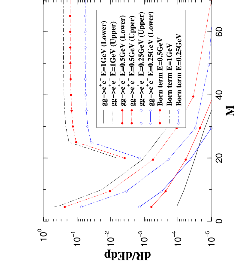
Figure 9: (Color online) Differential rate for the production of dileptons at high momenta and small invariant mass. See text for details.

It should be pointed out that such an expansion is only strictly valid as long as $\delta$ is of the order of the smallest scale in the problem i.e. $\frac{x}{E}$. However, as demonstrated by the plot of the imaginary part of the self energy in Fig. 8, it remains valid much beyond this point. This is due to the influence of the measure and the gluon distribution functions which drop rapidly as one moves away from $\delta=0$. It should be pointed out that only the matrix elements have been expanded in a series, all other factors (e.g.gluon distribution functions, measures etc. ) retain their closed expressions in $\delta$.

We are now in a position to integrate over $\delta$. This is also performed numerically. As we have expanded the matrix elements in $\delta$ and retained only a finite number of terms, the square of the matrix elements $|{\mathcal{M}}|^{2}$ grow beyond a certain $\delta=\delta_{1}$. This growth is not real and is merely a facet of our finite expansion in $\delta$. Two possible means of carrying out the $\delta$ integration present themselves. We may terminate the integral at $\delta_{1}$. Ostensibly, this represents the lower limit of the rate. These are represented in Fig. 9 as the solid lines (both with and without symbols). We may continue to integrate up to $\delta=\delta_{max}$; this will include the integration of a growing rate convoluted with an increasing angular measure ($\sin\delta$). This represents the upper limit of the rate. These are represented in Fig. 9 as the dotted lines. As the invariant mass is lowered or the energy of the pair is raised the differential rate drops sharply from its value at $\delta=0$; this invariably results in $m_{2}>>m_{1}$. As a result the integration beyond $\delta=\delta_{1}$ produces a large contribution; this in turn leads to the excess growth displayed by the upper limit at small invariant mass and large energies.

The rates after integration over $\delta$ are presented in Fig. 9. The dot-dashed lines are the rates from the Born term at various energies of the virtual photon. The solid lines are the lower limits of the rates from gluon gluon fusion for the respective energies of the virtual photon. The dotted lines are the upper limits of the respective rates. In general the rates from gluon gluon fusion are suppressed as compared to the Born term except at very high momenta or very low invariant mass. Three cases have been presented where the energy of the dilepton is set at 0.25, 0.5 and 1GeV. As may be noted, the results are quite similar to the back-to-back gluon fusion rates, i.e. the case at $\delta=0$. The rate from gluon fusion rises beyond the Born threshold due to the rising Bose-Einstein distributions of soft massless gluons.

VI Results for $m_{g}>0$

We now turn to the case where gluons acquire a medium-induced mass and where the virtual photon has no net three-momentum ($\vec{p}=0$). As we have seen, the gluon’s longitudinal degree of polarization allows to circumvent Yang’s theorem. More specifically, we expect transitions to occur when the net component of angular momentum is $\pm\hbar$:

$$\mathcal{M}_{i,j,3} = 0$$ (65)

$$\mathcal{M}_{\pm,3,\pm} = \mathcal{M}_{3,\pm,\pm}=-\frac{m_{g}}{k}\frac{eg^{2}\delta^{bc}}{2}\int\frac{dq}{(2\pi)^{2}}\Delta\widetilde{n}(E_{q},\mu)J(q,k)$$ (66)

where

$$J(q,k)=\frac{qk+\frac{q}{k}m_{g}^{2}}{8E_{k}E_{q}}\ln\left[\frac{(E_{q}E_{k}+qk)^{2}-\frac{m_{g}^{4}}{4}}{(E_{q}E_{k}-qk)^{2}-\frac{m_{g}^{4}}{4}}\right]-\frac{q}{4k}\ln\left[\frac{E_{q}^{2}E_{k}^{2}-\left(qk-\frac{m_{g}^{2}}{2}\right)^{2}}{E_{q}^{2}E_{k}^{2}-\left(qk+\frac{m_{g}^{2}}{2}\right)^{2}}\right]$$ (67)

where $E_{k}=\sqrt{k^{2}+m_{g}^{2}}$. Therefore, in the back–to–back configuration with massive and equally energetic gluons we find that the non-zero matrix elements are proportional to the gluon mass and scale like $\sim\mu$ confirming the finite density nature of this process. We point out that the integrand diverges unless $m_{g}<2m_{q}$. Beyond this limit the self-energy analytical structure becomes intricate. In this section, we present results only where the above relation holds. Dileptons production rates from regions beyond this threshold, as well as rates emanating from the fusion of massive gluons with $\vec{p}\neq 0$ will be addressed in a future effort maj04 .

To explore dilepton production in the range where the mass inequality is respected, we begin by ascribing current masses of 10 MeV to the quarks, setting the quark chemical potential to $\mu=40$ MeV, and the gluon mass to almost twice that of the quark (i.e. $m_{g}=19.99$ MeV) as a reference point. With these, we see that the differential production rate due to the gluon fusion is lower than the contribution from the Born term across the range of invariant mass (see Fig. 10). However, if we increase the quark chemical potential to $\mu=200$ MeV or reduce the quark current mass to $m_{q}=1$ MeV while maintaining the gluon to quark mass ratio (i.e. 1.999), we see that the gluon fusion rate may dominate over the Born term up to an invariant mass of 125 MeV in the case where the quark chemical potential reaches 200 MeV. We also present results where the gluon mass is set equal to that of the quark (i.e. 10 MeV), in this case we see that the rate from the gluon fusion dominates at low invariant mass. If we lower the gluon mass beyond that of the quark then the process will have a non-vanishing contribution in a region forbidden for the $q\bar{q}$ process due to its threshold (see Fig. 11).

If instead of current masses, the quark masses are set to values of the order of $gT$ then we find the rate from gluon fusion to be suppressed as compared to the Born term (see Fig. 11). This is not unexpected as the gluons fuse through a quark triangle; the presence of large masses in the quark propagators leads to the rates being suppressed in this region of parameter space.

As in the case of gluon fusion with $\vec{p}\neq 0$, an interesting feature of the differential rate is its strong dependence on $\mu^{2}$ (Fig. 12) and its weak dependence on temperature and other energy scales: as the chemical potential increases, the rate rises. For the Born term the opposite behaviour is true. As the chemical potential increases, the antiquark population is depleted, inhibiting the production of dileptons through this channel. Thus, an accurate estimate of the differential rate will require a good knowledge of the baryon chemical potential as well as its variation with time in a QGP.

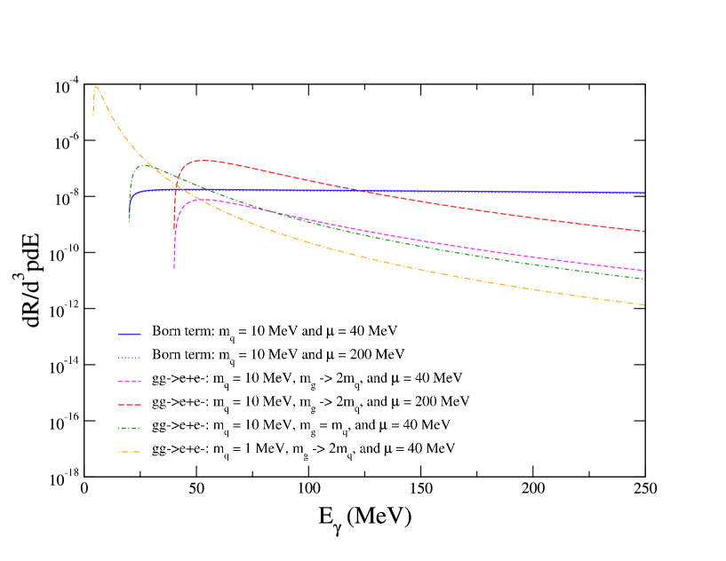
Figure 10: (Color online) Differential production rates for $T=400$ MeV. See text for details

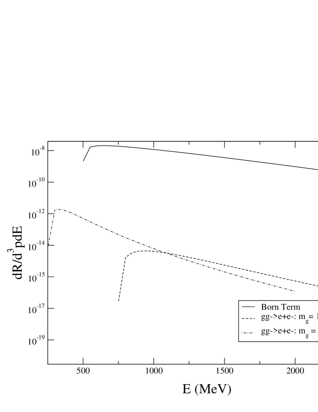
Figure 11: Differential production rates for $2g\rightarrow l\bar{l}$ with $T=400$ MeV, $\mu_{q}=40$ MeV, $m_{q}=250$ MeV, and different gluon masses.

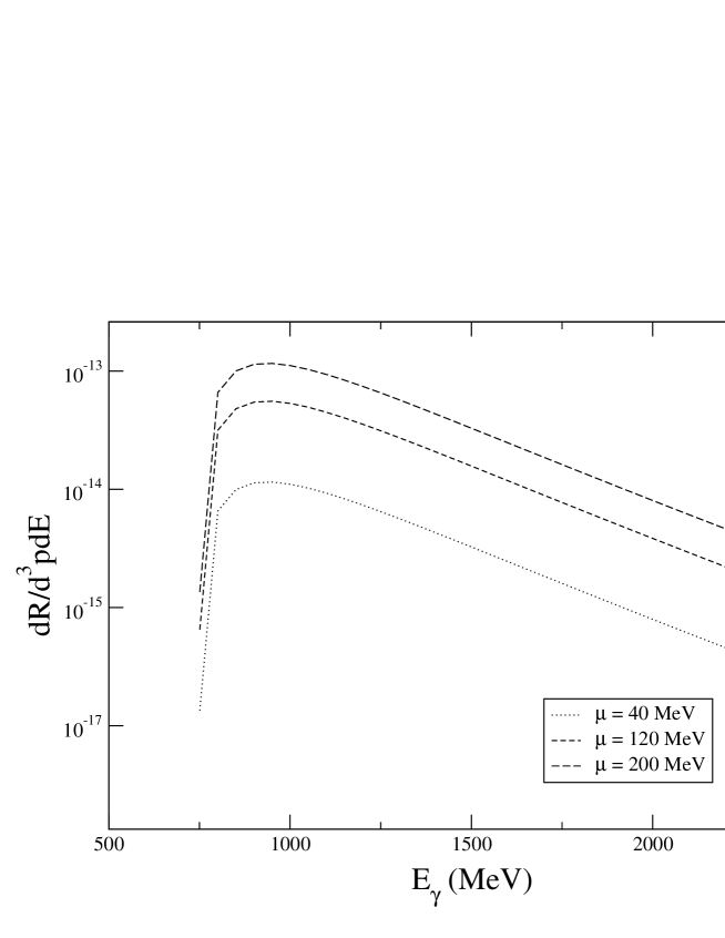
Figure 12: $\mu^{2}$ scaling of the differential production rates with $T=400$ MeV, $m_{q}=250$ MeV and $m_{g}=1.5m_{q}$ MeV.

VII Discussions and Conclusions

In this article we have presented a detailed study of the observational effects of broken charge conjugation, and broken rotational invariance in a QGP formed in a heavy-ion collision. The signal under consideration was the spectrum of dileptons emanating from such a medium. The reason behind this choice is evident: electromagnetic signatures provide a direct probe of all time sectors of a heavy-ion collision. The breaking of these symmetries is manifested at lowest order in the spectrum of dileptons produced by two gluon fusion into a virtual photon through a quark loop.

Such a process is forbidden in the vacuum by both Furry’s theorem and Yang’s theorem. Charge conjugation was broken explicitly by the introduction of a non-zero population of $u$ and $d$ valence quarks in the plasma. A non-zero baryon density, present solely in these flavours causes a net electric charge density in the medium. This leads to the breaking of Furry’s theorem which holds purely in neutral media.

The presence of a preferred rest frame of the medium leads to the introduction of a bath four-vector n into the problem. If calculations are performed in this frame then n$=(1,0,0,0)$. No such vector exists in the vacuum. If two massless back-to-back gluons with equal energy fuse in vacuum along the $z$-axis through the quark triangle, then the out state consisting of a static virtual photon will have the $z$ component of its spin $J_{z}=0$. Both in state and out state are eigenstates of a rotation by $\pi$ about the $x$-axis but have different eigenvalues. Hence such a transition is forbidden, this is the statement of Yang’s theorem and is based on the invariance of both in state and out state under a rotation by $\pi$ about the $x$-axis.

The above argument of no transition (due to the in state and out state possessing different eigenvalues with respect to the rotation by $\pi$ about the $x$-axis) continues to hold even for the production of a static photon in the rest frame of the bath where the in state and out state are modified to include spin-half fermions. It should be pointed out that we have tacitly assumed the plasma to be infinite in extent and isotropic; a realistic plasma of finite extent which is not spherically symmetric will explicitly break rotational invariance. To our knowledge, this fact may be understood solely in the spectator interpretation of loop diagrams. The spectator interpretation represents a formal procedure by which the imaginary part of a diagram containing loops may be re-expressed in terms of the product of matrix elements consisting solely of tree diagrams and particles from the bath that do not partake in the reaction process. The spectator interpretation for the imaginary part of a three-loop diagram was derived for this process and is essentially contained in Fig. 5. In the spectator interpretation different states containing fermions with different spins are added coherently. This allowed us to construct a subset of the entire sum of in states that respected the rotation symmetry of the vacuum state (see Eq. (48)). For each such subset no transition was allowed by arguments similar to those used in the construction of Yang’s theorem (see Sec. IV B).

This invariance will be broken by the presence of any three vector in the problem. The two possible choices for such a three-vector are a net three-momentum of the virtual photon ($\vec{p}\neq 0$ in the bath frame), or a non-zero $z$-component of its spin ($J_{z}\neq 0$). In the first case one may boost to the rest frame of the static photon. However, this will no longer be the rest frame of the plasma and rotational invariance will be explicitly broken. In the second case the production of a virtual photon with a $J_{z}\neq 0$ will require an incoming massive gluon which breaks one of the principal conditions required for Yang’s theorem to hold. In a real QGP we would expect both effects to be present simultaneously. In the interest of a clearer understanding of the mechanism of symmetry breaking we had chosen to explore both possibilities in isolation.

In the case of a virtual photon with a net three-momentum $\vec{p}$, we began with the case of two massless gluons in a back-to-back configuration along the $z$-axis but with unequal energies. This resulted in a virtual photon with a net three-momentum along the $z$-axis. Under this kinematic restriction we present a closed analytical expression for the matrix element (see Eq. (LABEL:anal_sum)). The rates from this matrix element are plotted in Figs. 6 and 7 in comparison with the Born term. These figures represent the cases with plasma temperatures at 400 MeV and 800 MeV, corresponding to the cases of QGP formed at RHIC and LHC energies. We find as expected that the differential rate rises with increasing chemical potential $\mu$; two extreme cases with $\mu=0.1T$ and $\mu=0.5T$ have been explored. The rates however show a rather modest rise with increasing temperature. This has been pointed out earlier due to the vanishing of the $g^{2}T^{2}$ component in the HTL calculation of this loop diagram maj01b . The rates are also observed to rise with increasing three-momentum $|\vec{p}|$ (for a given fixed energy) as expected due to the breaking of Yang’s theorem. As the gluons are massless they continue to contribute into the region beyond the Born threshold (see Fig. 7). In this region, contributions originate from the fusion of a gluon carrying a large majority of the photons energy with an ultra-soft gluon carrying a tiny fraction of the photon energy. In fact the rising rate in the right panel of Fig. 7 is due to the Bose enhancement obtained from the distribution function of the soft gluon. The presence of a gluon dispersion relation or a gluon mass will lead to this rate reaching a maximum at a threshold set by twice the gluon mass.

Integrating over all incoming gluon angles turned out to be an involved procedure and led us to invoke an approximation scheme. At very small invariant mass, we noted that the gluon fusion rate is dominated by back-to-back gluon fusion. We thus expanded in the angle between the photon and the more energetic gluon $\delta$. Results for the differential rate per unit energy and per unit momentum $d^{2}R/dEdp$ have been presented in Fig. 9, in comparison with the Born term. As expected the rate from gluon-gluon fusion becomes comparable to the Born term only at very low invariant mass, for photon energies of 0.25, 0.5 and 1GeV. As noted in the previous section a large portion of the enhancement may be attributed solely to the lack of a mass for the gluons and Bose-Einstein distributions as opposed to a Fermi-Dirac distributions for the quarks.

In the case of a virtual photon with a net $J_{z}$, the possible choices are $J_{z}=\pm 1$. This requires one of the incoming gluons to be in a longitudinally polarized state. Hence, the gluons were endowed with a mass. One may ascribe the origin of such a mass to dispersion in the medium. As in the previous case, the rate is seen to rise sharply with increasing chemical potential. Due to analytic considerations, the quark mass ($m_{q}$) was always set to be larger than half the gluon mass ($m_{g}<2m_{q}$). In this kinematic region, the rates from gluon gluon fusion turned out to dominate over the Born term for low invariant masses of dileptons, if the quarks were chosen to be light $m_{q}<<T$. However, the rates were sub-dominant to the Born term for the production of dileptons with large invariant mass, or for quark masses $\sim gT$. We point out, that, in this calculation $T=400MeV$, hence, $g\sim 2$. Thus unlike the case for plasmas at very high temperature $gT\sim T$.

Gluons with masses at and above this threshold ($2m_{q}$) may decay into two quarks which are both simultaneously on shell. In the language of spectators, this corresponds to one of the propagators in the diagrams of Fig. 4 going on shell. The calculational and interpretive complications that arise from this situation are rather involved and represent a problem for the spectator interpretation. A preliminary calculation without the use of the spectator interpretation at this threshold in the limit of massless quarks and gluons found the rate to be large maj01 ; however these required the use of momentum cutoffs which did not respect the symmetry required by Yang’s theorem. As pointed out earlier this made the physical interpretation of these results unclear. The computation of the rates at and beyond this threshold will full quark and gluon dispersion relations at finite three-momentum and their interpretation in terms of the spectator picture will be dealt with in a subsequent calculation maj04 . Our goals in the present article have been to separately elucidate certain symmetries of the vacuum which are broken by a particular channel of dilepton production in a quark gluon plasma. For the purposes of simplicity we computed the rates from this channel for a plasma in complete thermal and chemical equilibrium. As the dileptons in this channel are produced essentially form the fusion of gluons, this process may display far greater significance in early plasmas which are estimated to be out of chemical equilibrium with large gluon populations. An accurate extimation of the full dilepton rate from this channel will require a two step process. One needs to combine the two effects of symmetry breaking discussed in this article. This rate will then have to be folded in with a realistic space-time model of the evolution of the plasma. Such a model will have to include an estimation of the early gluon population with estimates for the effective inmedium masses of the gluons and the evolution of these quantities with time. Work in this direction is currently in progress maj04 .

Appendix A Contour integration of $T^{\mu\nu\rho}$

In this appendix, we outline the formal calculation of the two gluon photon vertex in the imaginary time formalism, using the method of contour integration. In this case, the standard method of contour integration will be modified to allow for the appearance of expressions which may be easily generalized from the case at zero density. This procedure allows for the construction of the spectator interpretation. As mentioned before in Eqs. (7) and (8) the Feynman rules for the two-gluon-photon vertex in the imaginary time formalism are,

$$\mathcal{T}^{\mu\nu\rho} = \frac{-1}{\beta}\int\frac{d^{3}q}{(2\pi)^{3}}\sum_{n}\mbox{Tr}\left[\frac{\mbox{}}{\mbox{}}\right.ie\delta_{ki}\gamma^{\mu}\frac{i(\not\!{\bf q}+m)}{{\bf q}^{2}-m^{2}}igt^{b}_{ij}\gamma^{\nu}$$ (68)

$$\times \frac{i(\not\!{\bf q}-\not\!{\bf k}+m)}{({\bf q}-{\bf k})^{2}-m^{2}}igt^{c}_{jk}\gamma^{\rho}\frac{i(\not\!{\bf q}-\not\!{\bf p}+m)}{({\bf q}-{\bf p})^{2}-m^{2}}\left.\frac{\mbox{}}{\mbox{}}\right]$$

$$\mathcal{T}^{\mu\rho\nu} = \frac{-1}{\beta}\int\frac{d^{3}q}{(2\pi)^{3}}\sum_{n}\mbox{Tr}\left[\frac{\mbox{}}{\mbox{}}\right.ie\delta_{ik}\gamma^{\mu}\frac{i(\not\!{\bf q}+\not\!{\bf p}+m)}{({\bf q}+{\bf p})^{2}-m^{2}}igt^{c}_{kj}\gamma^{\rho}$$ (69)

$$\times \frac{i(\not\!{\bf q}+\not\!{\bf k}+m)}{({\bf q}+{\bf k})^{2}-m^{2}}igt^{b}_{ji}\gamma^{\nu}\frac{i(\not\!{\bf q}+m)}{{\bf q}^{2}-m^{2}}\left.\frac{\mbox{}}{\mbox{}}\right]$$

Where the trace is implied over both colour and spin indices. The zeroth components of each four-momentum are

$$q^{0}=i(2n+1)\pi T+\mu,\mbox{\hskip 28.45274pt}p^{0}=i2m\pi T,\mbox{\hskip 28.45274pt}k^{0}=i2j\pi T.$$

where $n,m,j$ are integers, $\mu$ is the quark chemical potential. The overall minus sign is due to the fermion loop. The sum over $n$ runs over all integers from $-\infty$ to $+\infty$. As mentioned previously, the momentum dependent and mass dependent parts of the numerators of Eqs. (68) and (69) may be separated as

$$\mathcal{T}^{\mu\nu\rho} = \mathcal{B}^{\mu\alpha\nu\beta\rho\gamma}{\mathcal{T}_{1}}_{\alpha\beta\gamma}+\mathcal{A}_{1}^{\mu\nu\rho}=\frac{eg^{2}\delta^{bc}}{2\beta}\int\frac{d^{3}q}{(2\pi)^{3}}\sum_{n}\mbox{Tr}$$ (70)

$$\Bigg{[}\frac{\mathcal{B}^{\mu\alpha\nu\beta\rho\gamma}q_{\alpha}(q-k)_{\beta}(q-p)_{\gamma}}{({\bf q}^{2}-m^{2})(({\bf q}-{\bf k})^{2}-m^{2})(({\bf q}-{\bf p})^{2}-m^{2})}$$

$$+ m^{2}\frac{\mathcal{A}^{\mu\alpha\nu\rho}q_{\alpha}+\mathcal{A}^{\mu\nu\beta\rho}(q-k)_{\beta}+\mathcal{A}^{\mu\nu\rho\gamma}(q-p)_{\gamma}}{({\bf q}^{2}-m^{2})(({\bf q}-{\bf k})^{2}-m^{2})(({\bf q}-{\bf p})^{2}-m^{2})}\Bigg{]}$$

$$\mathcal{T}^{\mu\rho\nu} = \mathcal{B}^{\mu\alpha\rho\beta\nu\gamma}{\mathcal{T}_{2}}_{\alpha\beta\gamma}+\mathcal{A}_{2}^{\mu\nu\rho}=\frac{eg^{2}\delta^{bc}}{2\beta}\int\frac{d^{3}q}{(2\pi)^{3}}\sum_{n}\mbox{Tr}$$ (71)

$$\Bigg{[}\frac{\mathcal{B}^{\mu\alpha\rho\beta\nu\gamma}(q+p)_{\alpha}(q+k)_{\beta}(q)_{\gamma}}{({\bf q}^{2}-m^{2})(({\bf q}+{\bf k})^{2}-m^{2})(({\bf q}+{\bf p})^{2}-m^{2})}$$

$$+ m^{2}\frac{\mathcal{A}^{\mu\alpha\rho\nu}(q+p)_{\alpha}+\mathcal{A}^{\mu\rho\beta\nu}(q+k)_{\beta}+\mathcal{A}^{\mu\rho\nu\gamma}q_{\gamma}}{({\bf q}^{2}-m^{2})(({\bf q}+{\bf k})^{2}-m^{2})(({\bf q}+{\bf p})^{2}-m^{2})}\Bigg{]}$$

Where $\mathcal{A}^{\mu\nu\rho\gamma}$ represents the trace of four $\gamma$ matrices and $\mathcal{B}^{\mu\alpha\nu\beta\rho\gamma}$ represents the trace of six $\gamma$ matrices. Employing the methods of residue calculus, the sum over $n$ may be formally rewritten as a contour integration over the infinite set of contours $C_{1}$ (See Fig. 13)

$$T\sum_{n}f(q^{0}=i(2n+1)\pi T+\mu)=\frac{T}{2\pi i}\oint_{C_{1}}dq^{0}f(q^{0})\frac{1}{2}\beta\tanh\left(\frac{1}{2}\beta(q^{0}-\mu)\right)$$ (72)

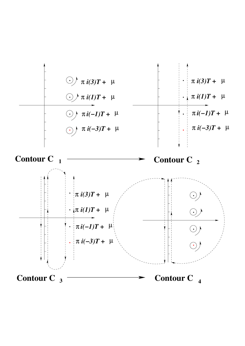
Figure 13: The contours used to evaluate the Matsubara sum with a finite chemical potential. See text for details.

The contours $C_{1}$ may be deformed to those of $C_{2}$ (see Fig. 13). These are a set of two linear contours meeting at $\pm i\infty$, one from $q^{0}=-i\infty+\mu+\epsilon\rightarrow q^{0}=i\infty+\mu+\epsilon$, and another from $i\infty+\mu-\epsilon\rightarrow-i\infty+\mu-\epsilon$. Here, and henceforth in all discussions of contours, residues and analytic continuations, $\epsilon$ will represent a vanishingly small quantity. One may now proceed by the standard method of kap89 and separate a vacuum part, thermal part and a pure density contribution. Instead, another set of contours is introduced: these run along the $y$ axis from $q^{0}=-i\infty+\epsilon\rightarrow q^{0}=i\infty+\epsilon$ and from $i\infty-\epsilon\rightarrow-i\infty-\epsilon$. Admittedly, as $\epsilon\rightarrow 0$ this contour will produce a vanishing contribution. The integrand in Eq. (68) has six powers of $q^{0}$ in the denominator and only three in the numerator. Hence it vanishes faster than a linear term as $q^{0}\rightarrow\infty$. As a result, this quantity obeys Jordan’s Lemma and the two integration contours around $0$ and $\mu$ may be connected by line segments at $\pm i\infty$. These line segments shown as curved lines in the third contour of Fig. 13 will have zero contribution to the entire integral. The total contour thus obtained is referred to as $C_{3}$. We now split the integrand into two, one piece for all the contours on the positive of the $x$ axis denoted as $C_{3}^{a}$, one piece for the sole contour on the negative side of the $x$ axis denoted as $C_{3}^{b}$, i.e.,

$$\frac{T}{2\pi i}\oint_{C_{1}}dq^{0}f(q^{0})\frac{1}{2}\beta\tanh\left(\frac{1}{2}\beta(q^{0}-\mu)\right) = \frac{1}{2\pi i}\int_{{i\infty-\epsilon}_{C_{3}^{b}}}^{-i\infty-\epsilon}dq^{0}f(q^{0})\left(-\frac{1}{2}+\frac{1}{e^{\beta(\mu-q^{0})}+1}\right)$$

$$\mbox{}+\frac{1}{2\pi i}\left(\int_{-i\infty+\epsilon}^{i\infty+\epsilon}+\int_{i\infty+\mu-\epsilon}^{-i\infty+\mu-\epsilon}+\int_{-i\infty+\mu+\epsilon}^{i\infty+\mu+\epsilon}\right)_{C_{3}^{a}} \!\!\!\!\!\!\!dq^{0}f(q^{0})\left(\frac{1}{2}-\frac{1}{e^{\beta(q^{0}-\mu)}+1}\right).$$ (73)

The terms may now be separated into a vacuum piece and a matter piece, note the similarity between this and the zero density separation. In this procedure, we differ from the standard method kap89 in not extracting an explicit finite density piece. The main reason for the extra contour deformation is to obtain the final answer in a form where the zero density contribution is obvious. In this spirit, we now reverse the direction of integration in $C_{3}^{b}$ and note that the vacuum piece has no poles at $i(2n+1)\pi T+\mu$. Thus the contours in the vacuum term may be allowed to overlap by setting $\epsilon=0$. We obtain

$$\frac{T}{2\pi i}\oint_{C_{1}}dq^{0}f(q^{0})\frac{1}{2}\beta\tanh\left(\frac{1}{2}\beta(q^{0}-\mu)\right)=\frac{1}{2\pi i}\int_{-i\infty}^{i\infty}dq^{0}f(q^{0})$$ (74)

$$+ \frac{1}{2\pi i}\int_{-i\infty-\epsilon}^{i\infty-\epsilon}dq^{0}f(q^{0})\frac{-1}{e^{\beta(-q^{0}+\mu)}+1}$$

$$+ \left(\int_{-i\infty+\epsilon}^{i\infty+\epsilon}+\int_{i\infty+\mu-\epsilon}^{-i\infty+\mu-\epsilon}+\int_{-i\infty+\mu+\epsilon}^{i\infty+\mu+\epsilon}\right)dq^{0}f(q^{0})\frac{-1}{e^{\beta(q^{0}-\mu)}+1}.$$

We now let $\epsilon\rightarrow 0$ on the contours on the positive side of the $x$ axis. This procedure will deform the two linear contours at $\mu\pm\epsilon$ back to the small circles around the points $i(2n+1)\pi T$, this part will become similar to the initial contour $C_{1}$. The rest of the contour can be closed by including the infinite arc in the $q^{0}=+\infty$ direction in the clockwise sense. This multiply connected contour is indicated as $C_{4}^{a}-C_{1}$ and displayed on the right of the fourth plot in Fig. 13. The linear contour on the negative side may be closed off as always by the infinite arc extending to $q^{0}=-\infty$. This is indicated as $C_{4}^{b}$ and shown as the left contour in the fourth plot of the figure. The contour integration over either contour may be replaced by the sum over all the residues at all the poles enclosed by the contour. Note that the poles at $i(2n+1)\pi T+\mu$, excluded by the multiply connected contour, are not to be included in the sum over residues. Thus our final, formal result is,

$$\!\!\!\!\!\!\!\!\!\!\!\frac{T}{2\pi i}\oint_{C_{1}}dq^{0}f(q^{0})\frac{1}{2}\beta\tanh\left(\frac{1}{2}\beta(q^{0}-\mu)\right) = \frac{1}{2\pi i}\int_{-i\infty}^{i\infty}dq^{0}f(q^{0})$$

$$-\sum_{i} \!\!\!\!\!\theta(-\omega_{i})\mbox{Res.}[f(q^{0})]\frac{1}{e^{\beta(-q^{0}+\mu)}+1}\Bigg{|}_{q^{0}=\omega_{i}}$$

$$+\sum_{i} \!\!\!\!\!\theta(\omega_{i})\mbox{Res.}[f(q^{0})]\frac{1}{e^{\beta(q^{0}-\mu)}+1}\Bigg{|}_{q^{0}=\omega_{i}}.$$ (75)

We may substitute the full integrand in Eq. (68) to obtain the result of contour integration as

$$\mathcal{T}^{\mu\nu\rho} = \frac{1}{2\pi i}\int_{-i\infty}^{i\infty}dq^{0}\int\frac{d^{3}q}{(2\pi)^{3}}\Bigg{[}\frac{eg^{2}\delta^{bc}}{2\beta}\Bigg{(}\frac{\mathcal{B}^{\mu\nu\rho}_{\alpha\beta\gamma}q^{\alpha}(q-k)^{\beta}(q-p)^{\gamma}}{({\bf q}^{2}-m^{2})(({\bf q}-{\bf k})^{2}-m^{2})(({\bf q}-{\bf p})^{2}-m^{2})}$$ (76)

$$+ 4m^{2}\frac{g^{\mu\nu}(q-p-k)^{\rho}+g^{\mu\rho}(q-k+p)^{\nu}+g^{\nu\rho}(q+k-p)^{\mu}}{({\bf q}^{2}-m^{2})(({\bf q}-{\bf k})^{2}-m^{2})(({\bf q}-{\bf p})^{2}-m^{2})}\Bigg{)}$$

$$+ \sum_{i}\Bigg{\{}\left[\frac{\mbox{}}{\mbox{}}\right.\frac{\theta(\omega_{i})}{e^{\beta(q^{0}-\mu)}+1}-\frac{\theta(-\omega_{i})}{e^{\beta(-q^{0}+\mu)}+1}\left.\frac{\mbox{}}{\mbox{}}\right]$$

$$\times \frac{eg^{2}\delta^{bc}}{2\beta}\mbox{Res.}\Bigg{(}\frac{\mathcal{B}^{\mu\nu\rho}_{\alpha\beta\gamma}q^{\alpha}(q-k)^{\beta}(q-p)^{\gamma}}{({\bf q}^{2}-m^{2})(({\bf q}-{\bf k})^{2}-m^{2})(({\bf q}-{\bf p})^{2}-m^{2})}$$

$$+ 4m^{2}\frac{g^{\mu\nu}(q-p-k)^{\rho}+g^{\mu\rho}(q-k+p)^{\nu}+g^{\nu\rho}(q+k-p)^{\mu}}{({\bf q}^{2}-m^{2})(({\bf q}-{\bf k})^{2}-m^{2})(({\bf q}-{\bf p})^{2}-m^{2})}\Bigg{)}\Bigg{\}}_{q^{0}=\omega_{i}}\Bigg{]}.$$

A similar contour analysis as above may be performed for Eq. (69), with the added extra step of setting $q^{0}\rightarrow-q^{0},\vec{q}\rightarrow-\vec{q}$. This procedure will produce a final contour of integration which is a mirror image of $C_{4}$. There will, once again, be an infinite semi-circle extending to $+\infty$ connected with the line running from $-i\infty+\epsilon\rightarrow i\infty+\epsilon$. There will also be an infinite semi-circle extending to $-\infty$ connected to the vertical line running on the negative side of the $x$ axis. This contour will however be multiply connected with the poles at $-i(2n+1)\pi T-\mu$ excluded from the region bounded by the infinite semi-circle. As before these poles shall be excluded from the sum over residues. Following this procedure, one obtains the result of the contour integration for Eq. (69) as,

$$\mathcal{T}^{\mu\rho\nu} = -\frac{1}{2\pi i}\int_{-i\infty}^{i\infty}dq^{0}\int\frac{d^{3}q}{(2\pi)^{3}}\Bigg{[}\frac{eg^{2}\delta^{bc}}{2\beta}\Bigg{(}\frac{\mathcal{B}^{\mu\nu\rho}_{\alpha\beta\gamma}q^{\alpha}(q-k)^{\beta}(q-p)^{\gamma}}{({\bf q}^{2}-m^{2})(({\bf q}-{\bf k})^{2}-m^{2})(({\bf q}-{\bf p})^{2}-m^{2})}$$ (77)

$$+ 4m^{2}\frac{g^{\mu\nu}(q-p-k)^{\rho}+g^{\mu\rho}(q-k+p)^{\nu}+g^{\nu\rho}(q+k-p)^{\mu}}{({\bf q}^{2}-m^{2})(({\bf q}-{\bf k})^{2}-m^{2})(({\bf q}-{\bf p})^{2}-m^{2})}\Bigg{)}$$

$$+ \sum_{i}\Bigg{\{}\left[\frac{\mbox{}}{\mbox{}}\right.\frac{\theta(\omega_{i})}{e^{\beta(q^{0}+\mu)}+1}-\frac{\theta(-\omega_{i})}{e^{\beta(-q^{0}-\mu)}+1}\left.\frac{\mbox{}}{\mbox{}}\right]$$

$$\times \frac{eg^{2}\delta^{bc}}{2\beta}\mbox{Res.}\Bigg{(}\frac{\mathcal{B}^{\mu\nu\rho}_{\alpha\beta\gamma}q^{\alpha}(q-k)^{\beta}(q-p)^{\gamma}}{({\bf q}^{2}-m^{2})(({\bf q}-{\bf k})^{2}-m^{2})(({\bf q}-{\bf p})^{2}-m^{2})}$$

$$+ 4m^{2}\frac{g^{\mu\nu}(q-p-k)^{\rho}+g^{\mu\rho}(q-k+p)^{\nu}+g^{\nu\rho}(q+k-p)^{\mu}}{({\bf q}^{2}-m^{2})(({\bf q}-{\bf k})^{2}-m^{2})(({\bf q}-{\bf p})^{2}-m^{2})}\Bigg{)}\Bigg{\}}_{q^{0}=\omega_{i}}\Bigg{]}.$$

Note, that the vacuum term is at least naively linearly divergent and thus the shift in momentum integrations may not be performed as above. However, from Furry’s theorem, one obtains that the sum of the vacuum terms from Eqs. (76) and (77) must be identically zero. Also note that the presence of the thermal distribution functions over quark momenta renders these integrals ultra-violet finite. Quark momentum shifts are thus definitely allowed for the thermal parts of Eqs. (76) and (77). Hence, We ignore the vacuum pieces and combine the matter pieces of both terms to obtain $T^{\mu\nu\rho}=\mathcal{T}^{\mu\nu\rho}+\mathcal{T}^{\mu\rho\nu}$ as,

$$T^{\mu\nu\rho} = \int\frac{d^{3}q}{(2\pi)^{3}}\sum_{i}\left[\frac{\mbox{}}{\mbox{}}\right.\theta(\omega_{i})\left(\frac{1}{e^{\beta(q^{0}-\mu)}+1}-\frac{1}{e^{\beta(q^{0}+\mu)}+1}\right)+\theta(-\omega_{i})\left(\frac{1}{e^{\beta(-q^{0}-\mu)}+1}-\frac{1}{e^{\beta(-q^{0}+\mu)}+1}\right)\left.\frac{\mbox{}}{\mbox{}}\right]$$ (78)

$$\times \frac{eg^{2}\delta^{bc}}{2\beta}\mbox{Res.}\Bigg{(}\frac{\mathcal{B}^{\mu\nu\rho}_{\alpha\beta\gamma}q^{\alpha}(q-k)^{\beta}(q-p)^{\gamma}}{({\bf q}^{2}-m^{2})(({\bf q}-{\bf k})^{2}-m^{2})(({\bf q}-{\bf p})^{2}-m^{2})}$$

$$+ 4m^{2}\frac{g^{\mu\nu}(q-p-k)^{\rho}+g^{\mu\rho}(q-k+p)^{\nu}+g^{\nu\rho}(q+k-p)^{\mu}}{({\bf q}^{2}-m^{2})(({\bf q}-{\bf k})^{2}-m^{2})(({\bf q}-{\bf p})^{2}-m^{2})}\Bigg{)}\Bigg{|}_{q^{0}=\omega_{i}}$$

References

- (1) E. Shuryak, Phys. Rep. 80, 71 (1980).
- (2) K. Kajantie, J. Kapusta, L. McLerran, and A. Mekjian, Phys. Rev. D. 34, 2746 (1986).
- (3) P. Aurenche, F. Gelis, G.D. Moore, and H. Zaraket, JHEP 0212 006 (2002).
- (4) Andrzej Olszewski et. al. J. Phys. G. 28, 1801 (2002).
- (5) A. Majumder, and C. Gale, Phys. Rev. D. 63 114008 (2001); Erratum-ibid. D. 64 119901 (2001).
- (6) W. H. Furry, Phys. Rev. 51 135 (1937).
- (7) A. Majumder, and C. Gale, Proc. MRST, London 2001, Theoretical high energy physics, 168 (2001).
- (8) J. I. Kapusta, Finite Temperature Field Theory, Cambridge University Press, (1989).
- (9) S. M. H. Wong, Phys. Rev. D. 64, 025007 (2001).
- (10) C. N. Yang, Phys. Rev. 77, 242 (1950).
- (11) C. Itzykson, J. B. Zuber, Quantum Field Theory, McGraw Hill, New York, (1980).
- (12) S. Weinberg, The Quantum Theory of Fields, Vol. 1, Cambridge University Press, (1995).
- (13) Particle data group, Eur. Phys. J. C. 3, 19 (1998).
- (14) See for example, S. A. Chin, Ann. Phys. 108, 301 (1977); H. A. Weldon, Phys. Lett. B 274, 133 (1992); O. Teodorescu, A. K. Dutt-Mazumder, and C. Gale, Phys. Rev. C 61, 051901 (2000).
- (15) R. D. Pisarski, Nucl. Phys. B309, 476 (1988).
- (16) J. I. Kapusta and S. M. H. Wong, Phys. Rev. D. 64, 045008 (2001).
- (17) A. Majumder and C. Gale, Phys. Rev. C. 65, 055203 (2002).
- (18) M. Le Bellac, Thermal Field Theory , Cambridge University Press, (1996).
- (19) S. M. H. Wong, Z. Phys. C. 53, 465 (1992).
- (20) X. N. Wang, Phys. Rept. 280, 287 (1997).
- (21) R. Rapp, Phys. Rev. C. 63, 054907 (2001).
- (22) J. I. Kapusta, and S. M. H. Wong, Phys. Rev. C. 62, 027901 (2000).
- (23) C. Gale, and J. I. Kapusta, Nucl. Phys. B357, 65 (1991).
- (24) K. Geiger, and J. I. Kapusta, Phys. Rev. D. 47, 4905 (1993).
- (25) K. J. Eskola, K. Kajantie, P. V. Ruuskanen and K. Tuominen, Nucl. Phys. B570, 379 (2000).
- (26) A. Majumder, A. Bourque and C. Gale, in preparation.