FIXED POLES, POLARIZED GLUE AND NUCLEON SPIN STRUCTURE

Abstract

We review the theory and present status of the proton spin problem with emphasis on possible gluonic and sea contributions. We discuss the possibility of a $J=1$ fixed pole correction to the Ellis-Jaffe sum rule for polarized deep inelastic scattering. Fixed poles in the real part of the forward Compton scattering amplitude have the potential to induce subtraction constant corrections to sum rules for photon nucleon scattering.

11.55.Hx, 13.60.Hb, 13.88.+e

1 Introduction

Understanding the spin structure of the proton is one of the most challenging problems facing subatomic physics: How is the spin of the proton built up out from the intrinsic spin and orbital angular momentum of its quark and gluonic constituents ? What happens to spin in the transition between current and constituent quarks in low-energy QCD. Key issues include the role of polarized glue and gluon topology in building up the spin of the proton.

Our present knowledge about the spin structure of the nucleon comes from polarized deep inelastic scattering. Following pioneering experiments at SLAC [1], recent experiments in fully inclusive polarized deep inelastic scattering have extended measurements of the nucleon’s $g_{1}$ spin dependent structure function to lower values of Bjorken $x$ where the nucleon’s sea becomes important [2]. From the first moment of $g_{1}$, these experiments have been interpreted to imply a small value for the flavour-singlet axial-charge:

$$g_{A}^{(0)}\bigr{|}_{\rm pDIS}=0.2-0.35.$$ (1)

This result is particularly interesting [3, 4] because $g_{A}^{(0)}$ is interpreted in the parton model as the fraction of the proton’s spin which is carried by the intrinsic spin of its quark and antiquark constituents. The value (1) is about half the prediction of relativistic constituent quark models ($\sim 60\%$). It corresponds to a negative strange-quark polarization

$$\Delta s=-0.10\pm 0.04$$ (2)

(polarized in the opposite direction to the spin of the proton).

The small value of $g_{A}^{(0)}|_{\rm pDIS}$ extracted from polarized deep inelastic scattering has inspired vast experimental and theoretical activity to understand the spin structure of the proton. New experiments are underway or being planned to map out the proton’s spin-flavour structure and to measure the amount of spin carried by polarized gluons in the polarized proton. These include semi-inclusive polarized deep inelastic scattering, polarized proton-proton collisions at RHIC [5], and polarized $ep$ collider studies [6]. Experiments at JLab will map out the valence region at large Bjorken $x$ (close to one) [7]. An independent, weak interaction, measurement of $g_{A}^{(0)}$ could be performed using elastic neutrino proton scattering [8]. Experiments with transversely polarized targets are just beginning and promise to reveal new information about the spin structure of the proton including tests of the Burkhardt-Cottingham sum rule for the nucleon’s $g_{2}$ spin structure function and measurements of a whole new family of “transversity observables”.

The plan of these lectures is as follows. We first summarise the phenomenology of the proton spin problem, including possible gluonic contributions. Next, in Sections 2 and 3, we give an overview of the derivation of the spin sum rules for polarized photon nucleon scattering, detailing the assumptions that are made at each step. Here we explain how these sum rules could be affected by potential subtraction constants (subtractions at infinity) in the dispersion relations for the spin dependent part of the forward Compton amplitude. We next give a brief review of fixed pole contributions to deep inelastic scattering in Section 4. Fixed poles are well known to play a vital role in the Adler sum rule for W-boson nucleon scattering [9] and the Schwinger term sum rule for the longitudinal structure function measured in unpolarized deep inelastic $ep$ scattering [10]. We explain how fixed poles could, in principle, affect the sum rules for the first moments of the $g_{1}$ and $g_{2}$ spin structure functions. For example, a subtraction constant correction to the Ellis-Jaffe sum rule for the first moment of the nucleon’s $g_{1}$ spin dependent structure function would follow if there is a real constant term in the spin dependent part of the forward deeply virtual Compton scattering amplitude. Section 5 discusses the QCD axial anomaly and its manifestation in $g_{A}^{(0)}$ and the spin structure of the proton. We conjecture that gluon topology may induce a $J=1$ fixed pole correction to the Ellis-Jaffe sum rule. Photon-gluon fusion and its importance to semi-inclusive measurements of sea polarization in polarized deep inelastic scattering are disussed in Section 6. A summary of key issues is given in Section 7.

1.1 The proton spin problem

First consider the flavour-singlet channel.

In QCD the axial anomaly [11] induces gluonic contributions to the flavour-singlet axial charge associated with the polarized glue in the nucleon and with gluon topology.

1. The first moment of the $g_{1}$ spin structure function for polarized photon-gluon fusion $(\gamma^{*}g\rightarrow q{\bar{q}})$ receives a negative contribution $-{\alpha_{s}\over 2\pi}$ from $k_{t}^{2}\sim Q^{2}$, where $k_{t}$ is the quark transverse momentum relative to the photon gluon direction and $Q^{2}$ is the virtuality of the hard photon [12, 13]. It also receives a positive contribution (proportional to the mass squared of the struck quark or antiquark) from low values of $k_{t}$, $k_{t}^{2}\sim P^{2},m^{2}$ where $P^{2}$ is the virtuality of the parent gluon and $m$ is the mass of the struck quark. The contact interaction ($k_{t}\sim Q$) between the polarized photon and gluon is flavour-independent, associated with the QCD axial anomaly and measures the spin of the target gluon. The mass dependent contribution is absorbed into the quark wavefunction of the nucleon.

2. Gluon topology is associated with gluonic boundary conditions and has the potential to induce a topological contribution to $g_{A}^{(0)}$ associated with Bjorken $x$ equal to zero: topological $x=0$ polarization or, essentially, a spin polarized condensate inside a nucleon [14].

Putting this physics together leads to the formula [12, 13, 14, 15]:

$$g_{A}^{(0)}=\biggl{(}\sum_{q}\Delta q-3{\alpha_{s}\over 2\pi}\Delta g\biggr{)}_{\rm partons}+{\cal C}$$ (3)

Here $\Delta g_{\rm partons}$ is the amount of spin carried by polarized gluon partons in the polarized proton and $\Delta q_{\rm partons}$ measures the spin carried by quarks and antiquarks carrying “soft” transverse momentum $k_{t}^{2}\sim m^{2},P^{2}$; ${\cal C}$ denotes the topological contribution. Since $\Delta g\sim 1/\alpha_{s}$ under QCD evolution, the polarized gluon term $[-{\alpha_{s}\over 2\pi}\Delta g]$ in Eq.(3) scales as $Q^{2}\rightarrow\infty$ [15].

Understanding the transverse momentum dependence of the quark and gluon contributions in Eq.(3) is essential to ensure that theory and experimental acceptance are correctly matched when extracting information from semi-inclusive measurements aimed at disentangling the individual valence, sea and gluonic contributions [16].

Since $x=0$ is inaccessible to deep inelastic scattering, the deep inelastic measurement of $g_{A}^{(0)}$, Eq.(1), is not necessarily inconsistent with the constituent quark model prediction 0.6 if a substantial fraction of the spin of the constituent quark is associated with gluon topology in the transition from constituent to current quarks (measured in polarized deep inelastic scattering) through dynamical axial U(1) symmetry breaking [4].

An “$x=0$” correction to deep inelastic measurements of $g_{A}^{(0)}$ would also follow if there is a leading twist “subtraction at infinity” in the dispersion relation for the spin dependent part of the forward Compton scattering amplitude (from a $J=1$ Regge fixed pole). An independent measurement of the flavour-singlet axial-charge through elastic neutrino proton scattering would be extremely valuable.

1.2 The isovector part of $g_{1}$

Quark model predictions for $g_{1}$ work much better in the isovector channel. The Bjorken sum rule which relates the first moment of $(g_{1}^{p}-g_{1}^{n})$ to the isovector axial charge $g_{A}^{(3)}$ measured in neutron beta decays has been confirmed at the level of 10% [2].

Looking beyond the first moment, the shape of $(g_{1}^{p}-g_{1}^{n})$ is very interesting. Figure 1 from Ref.[4] shows $2x(g_{1}^{p}-g_{1}^{n})$ (SLAC data) together with the isovector structure function $(F_{2}^{p}-F_{2}^{n})$ (NMC data). The ratio $R_{(3)}=2x(g_{1}^{p}-g_{1}^{n})/(F_{2}^{p}-F_{2}^{n})$ is plotted in Fig.2. It measures the ratio of polarized to unpolarized isovector quark distributions. The ratio $R_{(3)}$ is observed to be approximately constant (at the value $\sim 5/3$ predicted by SU(6) constituent quark models) for $x$ between 0.03 and 0.2, and goes towards one when $x\rightarrow 1$ (consistent with the predictions of QCD counting rules [17]). The area under $(F_{2}^{p}-F_{2}^{n})/2x$ is fixed by the Gottfried integral [18]. The observed shape of $g_{1}^{p}-g_{1}^{n}$ is almost required [4] in order to reproduce the area under the Bjorken sum rule, which is fixed by the value of $g_{A}^{(3)}$. The constant ratio in the low to medium $x$ range contrasts with the naive Regge prediction (strictly for $Q^{2}=0$) that the ratio $R_{(3)}$ should be roughly proportional to $x$ as $x\rightarrow 0$.

Figure 1: The isovector structure functions $2xg_{1}^{(p-n)}$ (SLAC data) and $F_{2}^{(p-n)}$ (NMC).

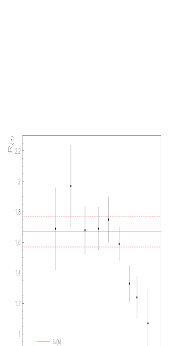
Figure 2: The ratio $R_{(3)}=2xg_{1}^{(p-n)}/F_{2}^{(p-n)}$.

2 Scattering amplitudes and cross-sections

The spin dependent structure functions $g_{1}$ and $g_{2}$ are defined through the imaginary part of the forward Compton scattering amplitude. Consider the amplitude for forward scattering of a photon carrying momentum $q_{\mu}$ ($q^{2}=-Q^{2}\leq 0$) from a polarized nucleon with momentum $p_{\mu}$, mass $M$ and spin $s_{\mu}$. Let $J_{\mu}(z)$ denote the electromagnetic current in QCD. The forward Compton amplitude

$$T_{\mu\nu}(q,p)=i\int d^{4}z\ e^{iq.z}\langle p,s|\ T(J_{\mu}(z)J_{\nu}(0))\ |p,s\rangle$$ (4)

is given by the sum of spin independent (symmetric in $\mu$ and $\nu$) and spin dependent (antisymmetric in $\mu$ and $\nu$) contributions:

$$T_{\mu\nu}^{S} = {1\over 2}(T_{\mu\nu}+T_{\nu\mu})$$ (5)

$$= -T_{1}(g_{\mu\nu}+{q_{\mu}q_{\nu}\over Q^{2}})+{1\over M^{2}}T_{2}(p_{\mu}+{p.q\over Q^{2}}q_{\mu})(p_{\nu}+{p.q\over Q^{2}}q_{\nu})$$

and

$$T_{\mu\nu}^{A} = {1\over 2}(T_{\mu\nu}-T_{\nu\mu})$$ (6)

$$= {i\over M^{2}}\epsilon_{\mu\nu\lambda\sigma}q^{\lambda}\biggl{[}s^{\sigma}(A_{1}+{\nu\over M}A_{2})-{1\over M^{2}}s.qp^{\sigma}A_{2}\biggr{]}$$

Here $\nu=p.q/M$, $\epsilon_{0123}=+1$, and the proton spin vector is normalized to $s^{2}=-1$. The form-factors $T_{1}$, $T_{2}$, $A_{1}$ and $A_{2}$ are functions of $\nu$ and $Q^{2}$.

The hadron tensor for inclusive photon nucleon scattering, which contains the spin dependent structure functions, is obtained from the imaginary part of $T_{\mu\nu}$:

$$W_{\mu\nu}={1\over\pi}{\rm Im}T_{\mu\nu}={1\over 2\pi}\int d^{4}z\ e^{iq.z}\langle p,s|\ [J_{\mu}(z),J_{\nu}(0)]\ |p,s\rangle$$ (7)

Here the connected matrix element is understood (indicating that the photon interacts with the target and not the vaccum). The spin independent and spin dependent components of $W_{\mu\nu}$ are

$$W_{\mu\nu}^{S}=-W_{1}(g_{\mu\nu}+{q_{\mu}q_{\nu}\over Q^{2}})+{1\over M^{2}}W_{2}(p_{\mu}+{p.q\over Q^{2}}q_{\mu})(p_{\nu}+{p.q\over Q^{2}}q_{\nu})$$ (8)

and

$$W_{\mu\nu}^{A}={i\over M^{2}}\epsilon_{\mu\nu\lambda\sigma}q^{\lambda}\biggl{[}s^{\sigma}(G_{1}+{\nu\over M}G_{2})-{1\over M^{2}}s.qp^{\sigma}G_{2}\biggr{]}$$ (9)

respectively. The cross sections for the absorption of a transversely polarized photon with spin polarized parallel $\sigma_{3\over 2}$ and anti-parallel $\sigma_{1\over 2}$ to the spin of the target nucleon are:

$$\sigma_{3\over 2} = {4\pi^{2}\alpha\over\sqrt{\nu^{2}+Q^{2}}}\biggl{[}W_{1}-{\nu\over M^{2}}G_{1}+{Q^{2}\over M^{3}}G_{2}\biggr{]}$$

$$\sigma_{1\over 2} = {4\pi^{2}\alpha\over\sqrt{\nu^{2}+Q^{2}}}\biggl{[}W_{1}+{\nu\over M^{2}}G_{1}-{Q^{2}\over M^{3}}G_{2}\biggr{]}$$ (10)

where we use usual conventions for the virtual photon flux factor [19]. The spin dependent part of the inclusive photon nucleon cross section is:

$$\sigma_{1\over 2}-\sigma_{3\over 2}={8\pi^{2}\alpha\over\sqrt{\nu^{2}+Q^{2}}}\biggl{[}{\nu\over M^{2}}G_{1}-{Q^{2}\over M^{3}}G_{2}\biggr{]}$$ (11)

For real photons ($Q^{2}=0$) this equation becomes $\{\sigma_{1\over 2}-\sigma_{3\over 2}={8\pi^{2}\alpha\over M^{2}}G_{1}\}$ — that is, $G_{2}$ decouples from polarized photoproduction. The $W_{2}$ structure function is measured in unpolarized lepton nucleon scattering through the absorption of longitudinally and transversely polarized photons. In high $Q^{2}$ deep inelastic scattering the structure functions exhibit approximate scaling:

$$M\ W_{1}(\nu,Q^{2}) \rightarrow F_{1}(x,Q^{2})$$

$$\nu\ W_{2}(\nu,Q^{2}) \rightarrow F_{2}(x,Q^{2})$$

$${\nu\over M}\ G_{1}(\nu,Q^{2}) \rightarrow g_{1}(x,Q^{2})$$

$${\nu^{2}\over M^{2}}\ G_{2}(\nu,Q^{2}) \rightarrow g_{2}(x,Q^{2})$$ (12)

Here $x={Q^{2}\over 2m\nu}$ is the Bjorken variable. The structure functions $F_{1}$, $F_{2}$, $g_{1}$ and $g_{2}$ scale modulo perturbative QCD logarithmic evolution in $Q^{2}$.

Regge theory makes predictions for the high-energy asymptotic behaviour of the structure functions:

$$W_{1} \sim\nu^{\alpha}$$ (13)

$$W_{2} \sim\nu^{\alpha-2}$$

$$G_{1} \sim\nu^{\alpha-1}$$

$$G_{2} \sim\nu^{\alpha-1}$$

Here $\alpha$ denotes the (effective) intercept for the leading Regge exchange contributions. The Regge predictions for the leading exchanges include $\alpha=1.08$ for the pomeron contributions to $W_{1}$ and $W_{2}$, and $\alpha\simeq 0.5$ for the $\rho$ and $\omega$ exchange contributions to the spin independent structure functions. For $G_{1}$ the leading gluonic exchange behaves as $\{\ln\nu\}/\nu$ [20, 21]; there are also isovector $a_{1}$ and isoscalar $f_{1}$ Regge exchanges [22]. If one makes the usual assumption that the $a_{1}$ and $f_{1}$ Regge trajectories are straight lines parallel to the $(\rho,\omega)$ trajectories then one finds $\alpha_{a_{1}}\simeq\alpha_{f_{1}}\simeq-0.4$, within the phenomenological range $-0.5\leq\alpha_{a_{1}}\leq 0$ [23]. For $G_{2}$ one expects contributions from possible multi-pomeron (three or more) cuts ($\sim(\ln\nu)^{-5}$) and Regge-pomeron cuts ($\sim\nu^{\alpha_{i}(0)-1}/\ln\nu$) with $\alpha_{i}(0)<1$ (since the pomeron does not couple to $A_{1}$ or $A_{2}$) [24]. The effective intercepts for small $x$, or high $\nu$, physics increase with increasing $Q^{2}$ through perturbative QCD evolution.

3 Dispersion Relations and Spin Sum Rules

Sum rules for the (spin) structure functions are derived using dispersion relations and, for deep inelastic scattering, the operator product expansion. For fixed $Q^{2}$ the forward Compton scattering amplitude $T_{\mu\nu}(\nu,Q^{2})$ is analytic in the photon energy $\nu$ except for branch cuts along the positive real axis for $|\nu|\geq Q^{2}/2M$. Crossing symmetry implies that

$$A_{1}^{*}(Q^{2},-\nu) = A_{1}(Q^{2},\nu)$$

$$A_{2}^{*}(Q^{2},-\nu) = -A_{2}(Q^{2},\nu)$$ (14)

The spin structure functions in the imaginary parts of $A_{1}$ and $A_{2}$ satisfy the crossing relations

$$G_{1}(Q^{2},-\nu) = -G_{1}(Q^{2},\nu)$$

$$G_{2}(Q^{2},-\nu) = +G_{2}(Q^{2},\nu)$$ (15)

For $g_{1}$ and $g_{2}$ these relations become

$$g_{1}(x,Q^{2}) = +g_{1}(-x,Q^{2})$$

$$g_{2}(x,Q^{2}) = +g_{2}(-x,Q^{2})$$ (16)

We use Cauchy’s integral theorem and the crossing relations to derive dispersion relations for $A_{1}$ and $A_{2}$. Assuming that the asymptotic behaviour of the spin structure functions $G_{1}$ and $G_{2}$ yield convergent integrals in an unsubtracted dispersion relation we are tempted to write unsubtracted dispersion relations:

$$A_{1}(Q^{2},\nu) = {2\over\pi}\int_{Q^{2}/2M}^{\infty}\ {\nu^{\prime}d\nu^{\prime}\over\nu^{\prime 2}-\nu^{2}}\ {\rm Im}A_{1}(Q^{2},\nu^{\prime})$$

$$A_{2}(Q^{2},\nu) = {2\over\pi}\nu\int_{Q^{2}/2M}^{\infty}\ {d\nu^{\prime}\over\nu^{\prime 2}-\nu^{2}}\ {\rm Im}A_{2}(Q^{2},\nu^{\prime})$$ (17)

These expressions can be rewritten as dispersion relations involving $g_{1}$ and $g_{2}$. We define:

$$\alpha_{1}(\omega,Q^{2}) = {\nu\over M}\ A_{1}$$

$$\alpha_{2}(\omega,Q^{2}) = {\nu^{2}\over M^{2}}\ A_{2}$$ (18)

Then, the formulae in (17) become

$$\alpha_{1}(\omega,Q^{2}) = 2\omega\int_{1}^{\infty}\ {d\omega^{\prime}\over\omega^{\prime 2}-\omega^{2}}\ g_{1}(\omega^{\prime},Q^{2})$$

$$\alpha_{2}(\omega,Q^{2}) = 2\omega^{3}\int_{1}^{\infty}\ {d\omega^{\prime}\over\omega^{\prime 2}(\omega^{\prime 2}-\omega^{2})}\ g_{2}(\omega^{\prime},Q^{2})$$ (19)

where $\omega={1\over x}={2M\nu\over Q^{2}}$.

In general there are two alternatives to an unsubtracted dispersion relation.

1. First, if the high energy behaviour of $G_{1}$ and/or $G_{2}$ (at some fixed $Q^{2}$) produced a divergent integral, then the dispersion relation would require a subtraction. Regge predictions for the high energy behaviour of $G_{1}$ and $G_{2}$ – see below Eq.(13) – each lead to convergent integrals so this scenario is not expected to occur.

2. Second, even if the integral in the unsubtracted relation converges, there is still the potential for a “subtraction at infinity”. This scenario would occur if the real part of $A_{1}$ and/or $A_{2}$ does not vanish sufficiently fast enough when $\nu\rightarrow\infty$ so that we pick up a finite contribution from the contour (or “circle at infinity”). In the context of Regge theory such subtractions can arise from fixed poles (with $J=\alpha(t)=0$ in $A_{2}$ or $J=\alpha(t)=1$ in $A_{1}$ for all $t$) in the real part of the forward Compton amplitude. We shall discuss these fixed poles and potential subtractions in Section 4.

In the presence of a potential “subtraction at infinity” the dispersion relations (17) are modified to:

$$A_{1}(Q^{2},\nu) = {\cal P}_{1}(\nu,Q^{2})+{2\over\pi}\int_{Q^{2}/2M}^{\infty}\ {\nu^{\prime}d\nu^{\prime}\over\nu^{\prime 2}-\nu^{2}}\ {\rm Im}A_{1}(q^{2},\nu^{\prime})$$

$$A_{2}(Q^{2},\nu) = {\cal P}_{2}(\nu,Q^{2})+{2\over\pi}\nu\int_{Q^{2}/2M}^{\infty}\ {d\nu^{\prime}\over\nu^{\prime 2}-\nu^{2}}\ {\rm Im}A_{2}(q^{2},\nu^{\prime})$$ (20)

Here

$${\cal P}_{1}(\nu,Q^{2}) = \beta_{1}(Q^{2})$$

$${\cal P}_{2}(\nu,Q^{2}) = \beta_{2}(Q^{2}){M\over\nu}$$ (21)

denote the subtraction constants. The crossing relations (14) for $A_{1}$ and $A_{2}$ are observed by the functions ${\cal P}_{i}$. Scaling requires that $\beta_{1}(Q^{2})$ and $\beta_{2}(Q^{2})$ (if finite) must be nonpolynomial in $Q^{2}$ – see Section 4. The equations (20) can be rewritten:

$$\alpha_{1}(\omega,Q^{2}) = {Q^{2}\over 2M^{2}}\ \beta_{1}(Q^{2})\ \omega+2\omega\int_{1}^{\infty}\ {d\omega^{\prime}\over\omega^{\prime 2}-\omega^{2}}\ g_{1}(\omega^{\prime},Q^{2})$$

$$\alpha_{2}(\omega,Q^{2}) = {Q^{2}\over 2M^{2}}\ \beta_{2}(Q^{2})\ \omega+2\omega^{3}\int_{1}^{\infty}\ {d\omega^{\prime}\over\omega^{\prime 2}(\omega^{\prime 2}-\omega^{2})}\ g_{2}(\omega^{\prime},Q^{2})$$ (22)

Next, the fact that both $\alpha_{1}$ and $\alpha_{2}$ are analytic for $|\omega|\leq 1$ allows us to make the Taylor series expansions (about $\omega=0$):

$$\alpha_{1}(x,Q^{2}) = {Q^{2}\over 2M^{2}}\ \beta_{1}(Q^{2})\ {1\over x}+{2\over x}\sum_{n=0,2,4,..}\biggl{(}{1\over x^{n}}\biggr{)}\int_{0}^{1}dy\ y^{n}g_{1}(y,Q^{2})$$

$$\alpha_{2}(x,Q^{2}) = {Q^{2}\over 2M^{2}}\ \beta_{2}(Q^{2})\ {1\over x}+{2\over x^{3}}\sum_{n=0,2,4,..}\biggl{(}{1\over x^{n}}\biggr{)}\int_{0}^{1}dy\ y^{n+2}g_{2}(y,Q^{2})$$

with $x={1\over\omega}$.

These equations form the basis for the spin sum rules for polarized photon nucleon scattering. We next outline the derivation of the Bjorken [25] and Ellis-Jaffe [26] sum rules for isovector and flavour-singlet parts of $g_{1}$ in polarized deep inelastic scattering, the Burkhardt-Cottingham sum rule for $G_{2}$ [27], and the Drell-Hearn-Gerasimov sum rule for polarized photoproduction [28]. Each of these spin sum rules assumes no subtraction at infinity.

3.1 Deep inelastic spin sum rules

Sum rules for polarized deep inelastic scattering are derived by combining the dispersion relation expressions (LABEL:eqcm) with the light cone operator production expansion. When $Q^{2}\rightarrow\infty$ the leading contribution to the spin dependent part of the forward Compton amplitude comes from the nucleon matrix elements of a tower of gauge invariant local operators multiplied by Wilson coefficients :

$$T_{\mu\nu}^{A}=i\epsilon_{\mu\nu\lambda\sigma}q^{\lambda}\sum_{n=0,2,4,..}\biggl{(}-{2\over q^{2}}\biggr{)}^{n+1}q^{\mu_{1}}q^{\mu_{2}}...q^{\mu_{n}}\sum_{i=q,g}\Theta^{(i)}_{\sigma\{\mu_{1}...\mu_{n}\}}E^{i}_{n}({Q^{2}\over\mu^{2}},\alpha_{s})$$ (24)

where

$$\Theta^{(q)}_{\sigma\{\mu_{1}...\mu_{n}\}}\equiv i^{n}\bar{\psi}\gamma_{\sigma}\gamma_{5}D_{\{\mu_{1}}...D_{\mu_{n}\}}\psi-{\rm traces}$$ (25)

and

$$\Theta^{(g)}_{\sigma\{\mu_{1}...\mu_{n}\}}\equiv i^{n-1}\epsilon_{\alpha\beta\gamma\sigma}G^{\beta\gamma}D_{\{\mu_{1}}...D_{\mu_{n-1}}G_{\ \mu_{n}\}}^{\alpha}-{\rm traces}$$ (26)

Here $D_{\mu}$ is the gauge covariant derivative and the sum over even values of $n$ in Eq.(24) reflects the crossing symmetry properties of $T_{\mu\nu}$. The functions $E^{q}_{n}({Q^{2}\over\mu^{2}},\alpha_{s})$ and $E^{g}_{n}({Q^{2}\over\mu^{2}},\alpha_{s})$ are the respective Wilson coeffients. The operators in Eq.(24) may each be written as the sum of a totally symmetric operator and an operator with mixed symmetry

$$\Theta_{\sigma\{\mu_{1}...\mu_{n}\}}=\Theta_{\{\sigma\mu_{1}...\mu_{n}\}}+\Theta_{[\sigma,\{\mu_{1}]...\mu_{n}\}}$$ (27)

These operators have the matrix elements:

$$\langle p,s|\Theta_{\{\sigma\mu_{1}...\mu_{n}\}}|p,s\rangle = \{s_{\sigma}p_{\mu_{1}}...p_{\mu_{n}}+s_{\mu_{1}}p_{\sigma}p_{\mu_{2}}...p_{\mu_{n}}+...\}{a_{n}\over n+1}$$

$$\langle p,s|\Theta_{[\{\sigma\mu_{1}]...\mu_{n}\}}|p,s\rangle = \{(s_{\sigma}p_{\mu_{1}}-s_{\mu_{1}}p_{\sigma})p_{\mu_{2}}...p_{\mu_{n}}$$ (28)

$$\ \ \ \ +(s_{\sigma}p_{\mu_{2}}-s_{\mu_{2}}p_{\sigma})p_{\mu_{1}}...p_{\mu_{n}}+...\}{d_{n}\over n+1}$$

Now define ${\tilde{a}}_{n}=a_{n}^{(q)}E_{1n}^{q}+a_{n}^{(g)}E_{1n}^{g}$ and ${\tilde{d}}_{n}=d_{n}^{(q)}E_{2n}^{q}+d_{n}^{(g)}E_{2n}^{g}$ where $E_{1n}^{i}$ and $E_{2n}^{i}$ are the Wilson coefficients for $a_{n}^{i}$ and $d_{n}^{i}$ respectively. Combining equations (24) and (28) one obtains equations for $\alpha_{1}$ and $\alpha_{2}$:

$$\alpha_{1}(x,Q^{2})+\alpha_{2}(x,Q^{2}) = \sum_{n=0,2,4,...}{{\tilde{a}}_{n}+n{\tilde{d}}_{n}\over n+1}{1\over x^{n+1}}$$

$$\alpha_{2}(x,Q^{2}) = \sum_{n=2,4,...}{n({\tilde{d}}_{n}-{\tilde{a}}_{n})\over n+1}{1\over x^{n+1}}$$ (29)

These equations are compared with the Taylor series expansions (LABEL:eqcm), whence we obtain the moment sum rules for $g_{1}$ and $g_{2}$:

$$\int_{0}^{1}dxx^{n}g_{1}={1\over 2}{\tilde{a}}_{n}$$ (30)

for $=0,2,4,...$ and

$$\int_{0}^{1}dxx^{n}g_{2}={1\over 2}{n\over n+1}({\tilde{d}}_{n}-{\tilde{a}}_{n})$$ (31)

for $n=2,4,6,...$
Note:

1. The first moment of $g_{1}$ is given by the nucleon matrix element of the axial vector current ${\bar{\psi}}\gamma_{\sigma}\gamma_{5}\psi$. There is no twist-two, spin-one, gauge-invariant, local gluon operator to contribute to the first moment of $g_{1}$ [29].

2. The potential subtraction term ${Q^{2}\over 2M}\beta_{1}(Q^{2})$ in the dispersion relation (22) multiplies a ${1\over x}$ term in the series expansion on the left hand side, and thus provides a potential correction factor to sum rules for the first moment of $g_{1}$. It follows that the first moment of $g_{1}$ measured in polarized deep inelastic scattering measures the nucleon matrix element of the axial vector current up to this potential “subtraction at infinity” term, which corresponds to the residue of any $J=1$ fixed pole with nonpolynomial residue contribution to the real part of $A_{1}$.

3. There is no ${1\over x}$ term in the operator product expansion formula (29) for $\alpha_{2}(x,Q^{2})$. This is matched by the lack of any ${1\over x}$ term in the unsubtracted version of the dispersion relation (LABEL:eqcm). The operator product expansion provides no information about the first moment of $g_{2}$ without additional assumptions concerning analytic continuation and the $x\sim 0$ behaviour of $g_{2}$ [30] — see the discussion about the Burkhardt Cottingham sum rule in Section 3.3.

If there are finite subtraction constant corrections to one (or more) spin sum rules, one can include the correction by re-interpreting the relevant structure function as a distribution with the subtraction constant included as the coefficient of a $\delta(x)$ term [10].

3.2 $g_{1}$ spin sum rules in polarized deep inelastic scattering

The value of $g_{A}^{(0)}$ extracted from polarized deep inelastic scattering is obtained as follows. One includes the sum over quark charges squared in $W_{\mu\nu}$ and assumes no twist-two subtraction constant ($\beta_{1}(Q^{2})=O(1/Q^{4})$). The first moment of the structure function $g_{1}$ is then related to the scale-invariant axial charges of the target nucleon by

$$\int_{0}^{1}dx\ g_{1}^{p}(x,Q^{2}) = \Biggl{(}{1\over 12}g_{A}^{(3)}+{1\over 36}g_{A}^{(8)}\Biggr{)}\Bigl{\{}1+\sum_{\ell\geq 1}c_{{\rm NS}\ell\,}\alpha_{s}^{\ell}(Q)\Bigr{\}}$$ (32)

$$+ {1\over 9}g_{A}^{(0)}|_{\rm inv}\Bigl{\{}1+\sum_{\ell\geq 1}c_{{\rm S}\ell\,}\alpha_{s}^{\ell}(Q)\Bigr{\}}\ +\ {\cal O}({1\over Q^{2}}).$$

Here $g_{A}^{(3)}$, $g_{A}^{(8)}$ and $g_{A}^{(0)}|_{\rm inv}$ are the isovector, SU(3) octet and scale-invariant flavour-singlet axial charges respectively. The flavour non-singlet $c_{{\rm NS}\ell}$ and singlet $c_{{\rm S}\ell}$ Wilson coefficients are calculable in $\ell$-loop perturbative QCD [31].

Note that the first moment of $g_{1}$ is constrained by low energy weak interactions. For proton states $|p,s\rangle$ with momentum $p_{\mu}$ and spin $s_{\mu}$

$$2ms_{\mu}\ g_{A}^{(3)} = \langle p,s|\left(\bar{u}\gamma_{\mu}\gamma_{5}u-\bar{d}\gamma_{\mu}\gamma_{5}d\right)|p,s\rangle$$

$$2ms_{\mu}\ g_{A}^{(8)} = \langle p,s|\left(\bar{u}\gamma_{\mu}\gamma_{5}u+\bar{d}\gamma_{\mu}\gamma_{5}d-2\bar{s}\gamma_{\mu}\gamma_{5}s\right)|p,s\rangle$$ (33)

Here $g_{A}^{\scriptscriptstyle(3)}=1.267\pm 0.004$ is the isovector axial charge measured in neutron beta-decay; $g_{A}^{\scriptscriptstyle(8)}=0.58\pm 0.03$ is the octet charge measured independently in hyperon beta decays (using SU(3)) [32]. (The assumption of good SU(3) here is supported by the recent KTeV measurement [33] of the $\Xi^{0}$ beta decay $\Xi^{0}\rightarrow\Sigma^{+}e{\bar{\nu}}$.)

The scale-invariant flavour-singlet axial charge $g_{A}^{(0)}|_{\rm inv}$ is defined by

$$2ms_{\mu}g_{A}^{(0)}|_{\rm inv}=\langle p,s|\ E(\alpha_{s})J^{GI}_{\mu 5}\ |p,s\rangle$$ (34)

where

$$J^{GI}_{\mu 5}=\left(\bar{u}\gamma_{\mu}\gamma_{5}u+\bar{d}\gamma_{\mu}\gamma_{5}d+\bar{s}\gamma_{\mu}\gamma_{5}s\right)_{GI}$$ (35)

is the gauge-invariantly renormalized singlet axial-vector operator and

$$E(\alpha_{s})=\exp\int^{\alpha_{s}}_{0}\!d{\tilde{\alpha}_{s}}\,\gamma({\tilde{\alpha}_{s}})/\beta({\tilde{\alpha}_{s}})$$ (36)

is a renormalization group factor which corrects for the (two loop) non-zero anomalous dimension $\gamma(\alpha_{s})$ ($=f{\alpha_{s}^{2}\over\pi^{2}}+{\cal O}(\alpha_{s}^{3})$) of $J_{\mu 5}^{GI}$ [34]. Here $\beta(\alpha_{s})$ is the QCD beta function. We are free to choose the QCD coupling $\alpha_{s}(\mu)$ at either a hard or a soft scale $\mu$. The singlet axial charge $g_{A}^{(0)}|_{\rm inv}$ is independent of the renormalization scale $\mu$ and corresponds to $g_{A}^{(0)}(Q^{2})$ evaluated in the limit $Q^{2}\rightarrow\infty$. If we take $\alpha_{s}(\mu_{0}^{2})\sim 0.6$ as typical of the infrared region of QCD, then the renormalization group factor $E(\alpha_{s})\simeq 1-0.13-0.03=0.84$ where -0.13 and -0.03 are the ${\cal O}(\alpha_{s})$ and ${\cal O}(\alpha_{s}^{2})$ corrections respectively.

In the isovector channel the Bjorken sum rule [25, 31]

$$I_{Bj}=\int_{0}^{1}dx\Biggl{(}g_{1}^{p}-g_{1}^{n}\Biggr{)}=\frac{g_{A}^{(3)}}{6}\left[1-\frac{\alpha_{s}}{\pi}-3.58\left(\frac{\alpha_{s}}{\pi}\right)^{2}-20.21\left(\frac{\alpha_{s}}{\pi}\right)^{3}\right]$$ (37)

has been confirmed at the level of 10%. Using the value $g_{A}^{(8)}=0.58\pm 0.03$ from hyperon beta-decays (and assuming no subtraction constant correction) the polarized deep inelastic data implies

$$\left.g^{(0)}_{A}\right|_{\rm pDIS}=0.2-0.35$$ (38)

for the flavour singlet (Ellis Jaffe) moment corresponding to the polarized strangeness $\Delta s=-0.10\pm 0.04$ quoted in Section 1.

The small $x$ extrapolation of $g_{1}$ data is presently the largest source of experimental error on measurements of the nucleon’s axial charges from deep inelastic scattering. We refer to Ziaja [35] for a recent discussion of perturbative QCD predictions for the small $x$ behaviour of $g_{1}$ in deep inelastic scattering.

Note that polarized deep inelastic scattering experiments measure $g_{1}$ between some small but finite value $x_{\rm min}$ and an upper value $x_{\rm max}$ which is close to one. Deep inelastic measurements of $g_{A}^{(3)}$ and $g_{A}^{(0)}$ involve a smooth extrapolation of the $g_{1}$ data to $x=0$ which is motivated either by Regge theory or by perturbative QCD. As we decrease $x_{\rm min}\rightarrow 0$ we measure the first moment

$$\Gamma\equiv\lim_{x_{\rm min}\rightarrow 0}\ \int^{1}_{x_{\rm min}}dx\ g_{1}(x,Q^{2}).$$ (39)

Polarized deep inelastic experiments cannot, even in principle, measure at $x=0$ with finite $Q^{2}$. They miss any possible $\delta(x)$ terms which might exist in $g_{1}$ at large $Q^{2}$. That is, they miss any potential (leading twist) fixed pole corrections and/or zero mode (topological) contributions to $g_{A}^{(0)}|_{\rm inv}$.

3.3 The Burkhardt Cottingham sum rule

The Burkhardt Cottingham sum rule [27] reads:

$$\int_{Q^{2}/2M}^{\infty}d\nu G_{2}(Q^{2},\nu)={2M^{3}\over Q^{2}}\int_{0}^{1}dxg_{2}=0$$ (40)

For deep inelastic scattering, this sum rule is derived by assuming that the moment formula (31) can be analytically continued to $n=0$. In general, the Burkhardt Cottingham sum rule is derived by assuming no $\alpha\geq 0$ singularity in $G_{2}$ (or, equivalently, no ${1\over x}$ or more singular small behaviour in $g_{2}$) and no “subtraction at infinity” (from an $\alpha=J=0$ fixed pole in the real part of $G_{2}$) [30]. The most precise measurements of $g_{2}$ to date in polarized deep inelastic scattering come from the SLAC E-155 and E-143 experiments, which report $\int_{0.02}^{0.8}dx\ g_{2}^{p}=-0.042\pm 0.008$ for the proton and $\int_{0.02}^{0.8}dx\ g_{2}^{d}=-0.006\pm 0.011$ for the deuteron at $Q^{2}=5$GeV² [36]. New, even more accurate, measurements of $g_{2}$ (for the neutron using a ³He target) are becoming available at Jefferson Laboratory [37] for $Q^{2}$ between 0.1 and 0.9 GeV². Further measurements to test the Burkhardt-Cottingham sum rule would be most valuable, particularly given the SLAC proton result quoted above.

3.4 The Drell Hearn Gerasimov sum rule

The Drell-Hearn-Gerasimov sum-rule [28] for spin dependent photoproduction relates the difference of the two cross-sections for the absorption of a real photon with spin anti-parallel $\sigma_{1\over 2}$ and parallel $\sigma_{3\over 2}$ to the target spin to the square of the anomalous magnetic moment of the target. It is derived by setting $\nu=0$ in the dispersion relation for $A_{1}$, Eq.(17). For small photon energy $\nu\rightarrow 0$

$$A_{1}(0,\nu)=-{1\over 4}\kappa^{2}+O(\nu^{2}),$$ (41)

where $\kappa$ is the anomalous magnetic moment of the target. This low-energy theorem follows from Lorentz invariance and electromagnetic gauge invariance (plus the existence of a finite mass gap between the ground state and continuum contributions to forward Compton scattering) [38, 39]. The Drell-Hearn-Gerasimov sum rule reads:

$$\int_{\rm threshold}^{\infty}{d\nu\over\nu}(\sigma_{1\over 2}-\sigma_{3\over 2})={8\pi^{2}\alpha\over M^{2}}\int_{\rm threshold}^{\infty}{d\nu\over\nu}G_{1}=-{2\pi^{2}\alpha\over M^{2}}\kappa^{2}$$ (42)

The sum rule follows from the very general principles of causality, unitarity, Lorentz and electromagnetic gauge invariance and one assumption: that the $g_{1}$ spin structure function satisfies an unsubtracted dispersion relation. Modulo the no-subtraction hypothesis, the Drell-Hearn-Gerasimov sum-rule is valid for a target of arbitrary spin $S$, whether elementary or composite [38] – for a review see [40].

The integral in Eq.(42) converges for each of the leading Regge contributions (discussed below Eq.(13)). If the sum rule were observed to fail (with finite integral) the interpretation would be a “subtraction at infinity” induced by a $J=1$ fixed pole in the real part of the spin amplitude $A_{1}$ [41].

Experimental investigations of the Drell-Hearn-Gerasimov sum rule are being carried out at several laboratories: ELSA and MAMI, JLab, GRAAL, LEGS@BNL, and SPRING. Preliminary results [42] from the ELSA-MAMI experiments suggest that the contribution to the DHG integral for a proton target from energies $\nu<3$GeV exceeds the total sum rule prediction (-204.5$\mu$b) by about 5-10%. Phenomenological estimates suggest that about $+25\pm 10\mu$b of the sum rule may reside at higher energies [43]. However it should be noted that any 10% fixed pole correction would be competitive with this high energy contribution within the errors. Further measurements, including at higher energy, would be valuable. These measurements could be carried out at SLAC or using a future polarized $ep$ collider [44]. In addition to mapping out spin dependent Regge theory and placing an upper bound on the the high energy contribution to the Drell-Hearn-Gerasimov sum rule high energy measurements of $G_{1}$ in polarized photoproduction would provide a baseline for investigations of perturbative QCD motivated small $x$ behaviour in $g_{1}$. The transition region between polarized photoproduction and deep inelastic $Q^{2}$ is expected to reveal much larger changes in the effective intercept for small $x$ physics than those observed in the unpolarized structure function $F_{2}$ [44].

4 Fixed Poles

Fixed poles are exchanges in Regge phenomenology with no $t$ dependence: the trajectories are described by $J=\alpha(t)=0$ or 1 for all $t$ [45]. For example, for fixed $Q^{2}$ a $t-$independent real constant term in the spin amplitude $A_{1}$ would correspond to a $J=1$ fixed pole. Fixed poles are excluded in hadron-hadron scattering by unitarity but are not excluded from Compton amplitudes (or parton distribution functions) because these are calculated only to lowest order in the current-hadron coupling. Indeed, there are two famous examples where fixed poles are required: (by current algebra) in the Adler sum rule for W-boson nucleon scattering, and to reproduce the Schwinger term sum rule for the longitudinal structure function measured in unpolarized deep inelastic $ep$ scattering. We review the derivation of these fixed pole contributions, and then discuss potential fixed pole corrections to the Burkhardt-Cottingham, $g_{1}$ and Drell-Hearn-Gerasimov sum-rules. Fixed poles in the real part of the forward Compton amplitude have the potential to induce “subtraction at infinity” corrections to sum rules for photon nucleon (or lepton nucleon) scattering. For example, a $\nu$ independent term in the real part of $A_{1}$ would induce a subtraction constant correction to the spin sum rule for the first moment of $g_{1}$. Bjorken scaling at large $Q^{2}$ constrains the $Q^{2}$ dependence of the residue of any fixed pole in the real of the forward Compton amplitide (e.g. $\beta_{1}(Q^{2})$ and $\beta_{2}(Q^{2})$ in the dispersion relations (22) ). To be consistent with scaling these residues must decay as or faster than $1/Q^{2}$ as $Q^{2}\to\infty$. That is, they must be nonpolynomial in $Q^{2}$.

4.1 Adler sum rule

The first example we consider is the Adler sum rule for W-boson nucleon scattering [9]:

$$\int_{Q^{2}/2M}^{+\infty}d\nu\biggl{[}W_{2}^{\bar{\nu}p}(\nu,Q^{2})-W_{2}^{\nu p}(\nu,Q^{2})\biggr{]} = \int_{0}^{1}{dx\over x}\biggl{[}F_{2}^{\bar{\nu}p}(x,Q^{2})-F_{2}^{\nu p}(x,Q^{2})\biggr{]}$$ (45)

$$= \begin{array}[]{c}4-2\cos^{2}\theta_{c}\ \ \ \ \ ({\rm BCT})\\ 2\ \ \ \ \ \ \ \ \ \ \ \ \ \ \ \ \ \ \ ({\rm ACT})\end{array}$$

Here $\theta_{c}$ is the Cabibbo angle, and BCT and ACT refer to below and above the charm production threshold.

The Adler sum rule is derived from current algebra. The right hand side of the sum rule is the coefficient of a $J=1$ fixed pole term

$${i\over\pi}f_{abc}\ F_{c}\ \biggl{[}(p_{\mu}q_{\nu}+q_{\mu}p_{\nu})-M\nu g_{\mu\nu}\biggr{]}/Q^{2}$$ (46)

in the imaginary part of the forward Compton amplitude for W-boson nucleon scattering [47]. This fixed pole term is required by the commutation relations between the charge raising and lowering weak currents

$$q_{\mu}T^{\mu\nu}_{ab} = -{1\over\pi}\int d^{4}x\ e^{iq.x}\ \langle p,s|\biggl{[}J_{a}^{0}(x),J^{\nu}_{b}(0)\biggr{]}|p,s\rangle\delta(x^{0})$$ (47)

$$= -{i\over\pi}f_{abc}\langle ps|J_{c}^{\nu}(0)|ps\rangle$$

Here $F_{c}$ is a generalized form factor at zero momentum transfer:

$$\langle p,s|J_{c}^{\nu}(0)|p,s\rangle\equiv p^{\nu}F_{c}$$ (48)

The fixed pole term appears in lowest order perturbation theory, and is not renormalized because it is a consequence of current algebra. The Adler sum rule is protected against radiative QCD corrections.

4.2 Schwinger term sum rule

Our second example is the Schwinger term sum rule [10] which relates the logarithmic integral in $\omega$ (or Bjorken $x$) of the longitudinal structure function $F_{L}(\omega,Q^{2})$ ($F_{L}={1\over 2}\omega F_{2}-F_{1}$) measured in unpolarized deep inelastic scattering to the target matrix element of the operator Schwinger term ${\cal S}$ defined through the equal-time commutator of the electromagnetic charge and current densities

$$\langle p,s|\biggl{[}J_{0}({\vec{y}},0),J_{i}(0)\biggr{]}|p,s\rangle=i\ \partial_{i}\ \delta^{3}({\vec{y}})\ {\cal S}.$$ (49)

The Schwinger term sum rule reads

$${\cal S}=\lim_{Q^{2}\rightarrow\infty}\biggl{[}4\int_{1}^{\infty}{d\omega\over\omega}{\tilde{F}}_{L}(\omega,Q^{2})-4\sum_{\alpha>0}\gamma(\alpha,Q^{2})/\alpha-C(q^{2})\biggr{]}$$ (50)

Here $C(Q^{2})$ is the nonpolynomial residue of any $J=0$ fixed pole contribution in the real part of $T_{2}$ and

$${\tilde{F}}_{L}(\omega,Q^{2})=F_{L}(\omega,Q^{2})-\sum_{\alpha\geq 0}\gamma(\alpha,Q^{2})\omega^{\alpha}.$$ (51)

The integral in Eq.(50) is convergent because ${\tilde{F}}_{L}(\omega,Q^{2})$ is defined with all Regge contributions with effective intecept greater than or equal to zero removed from $F_{L}(Q^{2},\omega)$. The Schwinger term ${\cal S}$ vanishes in vector gauge theories like QCD. Since $F_{L}(\omega,Q^{2})$ is positive definite, it follows that QCD possesses the required non-vanishing $J=0$ fixed pole in the real part of $T_{2}$.

4.3 Burkhardt Cottingham sum rule

The third example, and the first in connection with spin, is the Burkhardt Cottingham sum rule for the first moment of $g_{2}$ [27]:

$$\int_{Q^{2}/2M}^{\infty}d\nu\ G_{2}(Q^{2},\nu)={2M^{3}\over Q^{2}}\int_{0}^{1}dxg_{2}=0$$

Suppose that future experiments find that the sum rule is violated and that the integral is finite. The conclusion [30] would be a $J=0$ fixed pole with nonpolynomial residue in the real part of $A_{2}$. To see this work at fixed $Q^{2}$ and assume that all Regge-like singularities contributing to $A_{2}(\nu,Q^{2})$ have intercept less than zero so that

$$A_{2}(\nu,Q^{2})\sim\nu^{-1-\epsilon}$$ (52)

as $\nu\rightarrow\infty$ for some $\epsilon<0$. Then the large $\nu$ behaviour of $A_{2}$ is obtained by taking $\nu\rightarrow\infty$ under the $\nu^{\prime}$ integral giving

$$A_{2}(Q^{2},\nu)\sim-{2\over\pi\nu}\int_{Q^{2}/2M}^{\infty}d\nu^{\prime}\ {\rm Im}A_{2}(Q^{2},\nu^{\prime})$$ (53)

which contradicts the assumed behaviour unless the integral vanishes; hence the sum rule. If there is an $\alpha(0)=0$ fixed pole in the real part of $A_{2}$ the fixed pole will not contribute to ${\rm Im}A_{2}$ and therefore not spoil the convergence of the integral. One finds

$$\beta_{2}(Q^{2})\sim-{2\over\pi M}\int_{Q^{2}/2M}^{\infty}d\nu^{\prime}\ {\rm Im}A_{2}(Q^{2},\nu^{\prime})$$ (54)

for the residue of any $J=0$ fixed pole coupling to $A_{2}(Q^{2},\nu)$.

4.4 $g_{1}$ spin sum rules

Scaling requires that any fixed pole correction to the Ellis Jaffe $g_{1}$ sum rule must have nonpolynomial residue. Through Eq.(LABEL:eqcm), the fixed pole coefficient $\beta_{1}(Q^{2})$ must decay as or faster than $O(1/Q^{2})$ as $Q^{2}\rightarrow\infty$. The coefficient is further constrained by the requirement that $G_{1}$ contains no kinematic singularities (for example at $Q^{2}=0$). In Section 5 we will identify a potential leading-twist topological $x=0$ contribution to the first moment of $g_{1}$ through analysis of the axial anomaly contribution to $g_{A}^{(0)}$. This zero-mode topological contribution (if finite) generates a leading twist fixed pole correction to the flavour-singlet part of $\int_{0}^{1}dxg_{1}$. If present, this fixed pole will also violate the Drell-Hearn-Gerasimov sum rule (since the two sum rules are derived from $A_{1}$) unless the underlying dynamics suppress the fixed pole’s residue at $Q^{2}=0$.

At this point it is interesting to consider the $g_{1}$ spin structure function of a polarized real photon. (Assuming no fixed pole correction) the first moment of $g_{1}^{\gamma}$ of a real photon vanishes

$$\int_{0}^{1}\ dx\ g_{1}^{\gamma}(x,Q^{2})=0$$ (55)

independent of the virtuality $Q^{2}$ of the photon that it is probed with [48, 49]. This result is non-perturbative. There are two derivations. In the first we treat the real photon as the beam and the virtual photon, and apply the Drell-Hearn-Gerasimov sum rule. The anomalous magnetic moment of a photon vanishes to all orders because of Furry’s theorem. Alternatively (for large $Q^{2}$), we can treat the deeply virtual photon as the beam and apply the operator product expansion. The sum rule (55) holds to all orders in perturbation theory and at every twist. If there is a fixed pole correction to the polarized real photon spin sum rule (55) then the correction will affect both the deep inelastic first moment (applied to the deeply virtual photon) and Drell-Hearn-Gerasimov (applied to the real photon) sum rules for the polarized photon system. Measurements of $g_{1}^{\gamma}$ might be possible with a polarized $e\gamma$ collider [50].

Note that any fixed pole correction to the Drell-Hearn-Gerasimov sum rule is most probably a non-perturbative effect. The sum rule (42) has been verified to $O(\alpha^{2})$ for all $2\rightarrow 2$ processes $\gamma a\rightarrow bc$ where $a$ is either a real lepton, quark, gluon or elementary Higgs target [51], and for electrons in QED to $O(\alpha^{3})$ [52].

One could test for a fixed pole correction to the Ellis-Jaffe moment through a precision measurement of the flavour singlet axial charge from an independent process where one is not sensitive to theoretical assumptions about the presence or absence of a $J=1$ fixed pole in $A_{1}$. Here the natural choice is elastic neutrino proton scattering [8, 53] where the parity violating part of the cross-section includes a direct weak interaction measurement of the scale invariant flavour-singlet axial charge $g_{A}^{(0)}|_{\rm inv}$, or through parity violation in light atoms [54, 55].

The subtraction constant fixed pole correction hypothesis could also, in principle, be tested through measurement of the real part of the spin dependent part of the forward deeply virtual Compton amplitude. While this measurement may seem extremely difficult at the present time one should not forget that Bjorken believed when writing his original Bjorken sum rule paper that the sum rule would never be tested [25]!

4.5 $\nu p$ elastic scattering

Neutrino proton elastic scattering measures the proton’s weak axial charge $g_{A}^{\mbox{$\scriptscriptstyle(Z)$}}$ through elastic Z⁰ exchange. Because of anomaly cancellation in the Standard Model the weak neutral current couples to the combination $u-d+c-s+t-b$, viz.

$$J_{\mu 5}^{Z}\ =\ \mbox{\small${\displaystyle\frac{1}{2}}$}\biggl{\{}\,\sum_{q=u,c,t}-\sum_{q=d,s,b}\,\biggr{\}}\>\bar{q}\gamma_{\mu}\gamma_{5}q$$ (56)

It measures the combination

$$2g_{A}^{\mbox{$\scriptscriptstyle(Z)$}}=\bigl{(}\Delta u-\Delta d-\Delta s\bigr{)}+\bigl{(}\Delta c-\Delta b+\Delta t\bigr{)}$$ (57)

where $\Delta q$ refers to the expectation value

$$\langle p,s|\,\bar{q}\gamma_{\mu}\gamma_{5}q\,|p,s\rangle=2Ms_{\mu}\Delta q$$

for a proton of spin $s_{\mu}$ and mass $M$. Heavy quark renormalization group arguments can be used to calculate the heavy $t$, $b$ and $c$ quark contributions to $g_{A}^{\mbox{$\scriptscriptstyle(Z)$}}$. The full NLO result is [56]

$$2g_{A}^{\mbox{$\scriptscriptstyle(Z)$}}\,=\,\bigl{(}\Delta u-\Delta d-\Delta s\bigr{)}_{\rm inv}+\hskip 0.56905pt{\cal H}\hskip 0.28453pt\bigl{(}\Delta u+\Delta d+\Delta s\bigr{)}_{\rm inv}+\,O(m_{t,b,c}^{-1})$$ (58)

where ${\cal H}$ is a polynomial in the running couplings $\widetilde{\alpha}_{h}$,

$${\cal H}\,=\, \mbox{\small${\displaystyle\frac{6}{23\pi}}$}\bigl{(}\widetilde{\alpha}_{b}-\widetilde{\alpha}_{t}\bigr{)}\Bigl{\{}1+\mbox{\small${\displaystyle\frac{125663}{82800\pi}}$}\widetilde{\alpha}_{b}+\mbox{\small${\displaystyle\frac{6167}{3312\pi}}$}\widetilde{\alpha}_{t}-\mbox{\small${\displaystyle\frac{22}{75\pi}}$}\widetilde{\alpha}_{c}\Bigr{\}}$$ (59)

$$\phantom{+\ \Biggl{[}}-\mbox{\small${\displaystyle\frac{6}{27\pi}}$}\widetilde{\alpha}_{c}-\mbox{\small${\displaystyle\frac{181}{648\pi^{2}}}$}\widetilde{\alpha}_{c}^{2}+O\bigl{(}\widetilde{\alpha}_{t,b,c}^{3}\bigr{)}$$

Here $(\Delta q)_{\rm inv}$ denotes the scale-invariant version of $\Delta q$ and $\widetilde{\alpha}_{h}$ denotes Witten’s renormalization-group-invariant running couplings for heavy quark physics [57, 58]. Taking $\widetilde{\alpha}_{t}=0.1$, $\widetilde{\alpha}_{b}=0.2$ and $\widetilde{\alpha}_{c}=0.35$ in (59), one finds a small heavy-quark correction factor ${\cal H}=-0.02$, with LO terms dominant.

Modulo the small heavy-quark corrections quoted above, a precision measurement of $g_{A}^{(Z)}$, together with $g_{A}^{(3)}$ and $g_{A}^{(8)}$, would provide a weak interaction determination of $(\Delta s)_{\rm inv}$, complementary to the deep inelastic measurement (2). The $\nu p$ elastic measurement may be possible [8] at FNAL using the mini-BooNE set-up with small duty factor ($\sim 10^{-5}$) neutrino beam to control backgrounds. The estimated error on the strange quark polarization one could extract from this experiment is $\sim 0.03$, competitive with the error from present polarized deep inelastic measurements.

5 The axial anomaly, gluon topology and $g_{A}^{(0)}$

We next discuss the role of the axial anomaly in the interpretation of $g_{A}^{(0)}$.

5.1 The axial anomaly

In QCD one has to consider the effects of renormalization. The flavour singlet axial vector current $J_{\mu 5}^{GI}$ in Eq.(35) satisfies the anomalous divergence equation [11, 59]

$$\partial^{\mu}J^{GI}_{\mu 5}=2f\partial^{\mu}K_{\mu}+\sum_{i=1}^{f}2im_{i}\bar{q}_{i}\gamma_{5}q_{i}$$ (60)

where

$$K_{\mu}={g^{2}\over 32\pi^{2}}\epsilon_{\mu\nu\rho\sigma}\biggl{[}A^{\nu}_{a}\biggl{(}\partial^{\rho}A^{\sigma}_{a}-{1\over 3}gf_{abc}A^{\rho}_{b}A^{\sigma}_{c}\biggr{)}\biggr{]}$$ (61)

is a renormalized version of the gluonic Chern-Simons current and the number of light flavours $f$ is $3$. Eq.(60) allows us to write

$$J_{\mu 5}^{GI}=J_{\mu 5}^{\rm con}+2fK_{\mu}$$ (62)

where $J_{\mu 5}^{\rm con}$ and $K_{\mu}$ satisfy the divergence equations

$$\partial^{\mu}J^{\rm con}_{\mu 5}=\sum_{i=1}^{f}2im_{i}\bar{q}_{i}\gamma_{5}q_{i}$$ (63)

and

$$\partial^{\mu}K_{\mu}={g^{2}\over 32\pi^{2}}G_{\mu\nu}{\tilde{G}}^{\mu\nu}.$$ (64)

Here ${g^{2}\over 32\pi^{2}}G_{\mu\nu}{\tilde{G}}^{\mu\nu}$ is the topological charge density. The partially conserved current is scale invariant and the scale dependence of $J_{\mu 5}^{GI}$ is carried entirely by $K_{\mu}$. When we make a gauge transformation $U$ the gluon field transforms as

$$A_{\mu}\rightarrow UA_{\mu}U^{-1}+{i\over g}(\partial_{\mu}U)U^{-1}$$ (65)

and the operator $K_{\mu}$ transforms as

$$K_{\mu}\rightarrow K_{\mu}+i{g\over 8\pi^{2}}\epsilon_{\mu\nu\alpha\beta}\partial^{\nu}\biggl{(}U^{\dagger}\partial^{\alpha}UA^{\beta}\biggr{)}+{1\over 24\pi^{2}}\epsilon_{\mu\nu\alpha\beta}\biggl{[}(U^{\dagger}\partial^{\nu}U)(U^{\dagger}\partial^{\alpha}U)(U^{\dagger}\partial^{\beta}U)\biggr{]}.$$ (66)

Gauge transformations shuffle a scale invariant operator quantity between the two operators $J_{\mu 5}^{\rm con}$ and $K_{\mu}$ whilst keeping $J_{\mu 5}^{GI}$ invariant.

The nucleon matrix element of $J_{\mu 5}^{GI}$ is

$$\langle p,s|J^{GI}_{5\mu}|p^{\prime},s^{\prime}\rangle=2M\biggl{[}{\tilde{s}}_{\mu}G_{A}(l^{2})+l_{\mu}l.{\tilde{s}}G_{P}(l^{2})\biggr{]}$$ (67)

where $l_{\mu}=(p^{\prime}-p)_{\mu}$ and ${\tilde{s}}_{\mu}={\overline{u}}_{(p,s)}\gamma_{\mu}\gamma_{5}u_{(p^{\prime},s^{\prime})}/2M$. Since $J^{GI}_{5\mu}$ does not couple to a massless Goldstone boson it follows that $G_{A}(l^{2})$ and $G_{P}(l^{2})$ contain no massless pole terms. The forward matrix element of $J^{GI}_{5\mu}$ is well defined and

$$g_{A}^{(0)}|_{\rm inv}=E(\alpha_{s})G_{A}(0).$$ (68)

We would like to isolate the gluonic contribution to $G_{A}(0)$ associated with $K_{\mu}$ and thus write $g_{A}^{(0)}$ as the sum of (measurable) “quark” and “gluonic” contributions. Here one has to be careful because of the gauge dependence of the operator $K_{\mu}$. To understand the gluonic contributions to $g_{A}^{(0)}$ it is helpful to go back to the deep inelastic cross-section in Section 2.

5.2 The anomaly and the first moment of $g_{1}$

We specialise to the target rest frame and let $E$ denote the energy of the incident charged lepton which is scattered through an angle $\theta$ to emerge in the final state with energy $E^{\prime}$. Let $\uparrow\downarrow$ denote the longitudinal polarization of the beam and $\Uparrow\Downarrow$ denote a longitudinally polarized proton target. The spin dependent part of the differential cross-sections is:

$$\Biggl{(}{d^{2}\sigma\uparrow\Uparrow\over d\Omega dE^{{}^{\prime}}}-{d^{2}\sigma\uparrow\Downarrow\over d\Omega dE^{{}^{\prime}}}\Biggr{)}={4\alpha^{2}E^{{}^{\prime}}\over Q^{2}E\nu}\biggl{[}(E+E^{{}^{\prime}}\cos\theta)\ g_{1}(x,Q^{2})-{2xM}\ g_{2}(x,Q^{2})\biggr{]}$$ (69)

which is obtained from the product of the lepton and hadron tensors:

$${d^{2}\sigma\over d\Omega dE^{\prime}}={\alpha^{2}\over Q^{4}}{E^{\prime}\over E}\ L_{\mu\nu}^{A}\ W^{\mu\nu}_{A}$$ (70)

Here the lepton tensor

$$L_{\mu\nu}^{A}=2i\epsilon_{\mu\nu\alpha\beta}k^{\alpha}q^{\beta}$$ (71)

describes the lepton-photon vertex and the hadronic tensor

$${1\over M}W^{\mu\nu}_{A}=i\epsilon^{\mu\nu\rho\sigma}q_{\rho}\biggl{(}s_{\sigma}{1\over p.q}g_{1}(x,Q^{2})+[p.qs_{\sigma}-s.qp_{\sigma}]{1\over M^{2}p.q}g_{2}(x,Q^{2})\biggr{)}$$ (72)

describes the photon-nucleon interaction.

Deep inelastic scattering involves the Bjorken limit: $Q^{2}=-q^{2}$ and $p.q=M\nu$ both $\rightarrow\infty$ with $x={Q^{2}\over 2M\nu}$ held fixed. In terms of light-cone coordinates this corresponds to taking $q_{-}\rightarrow\infty$ with $q_{+}=-xp_{+}$ held finite. The leading term in $W_{A}^{\mu\nu}$ is obtained by taking the Lorentz index of $s_{\sigma}$ as $\sigma=+$. (Other terms are suppressed by powers of ${1\over q_{-}}$.)

The flavour-singlet axial charge which is measured in the first moment of $g_{1}$ is given by the matrix element

$$2Ms_{\mu}g_{A}^{(0)}=\langle p,s|J^{GI}_{\mu 5}|p,s\rangle$$

If we wish to understand the first moment of $g_{1}$ in terms of the matrix elements of anomalous currents ($J_{\mu 5}^{\rm con}$ and $K_{\mu}$), then we have to understand the forward matrix element of $K_{+}$.

Here we are fortunate in that the parton model is formulated in the light-cone gauge ($A_{+}=0$) where the forward matrix elements of $K_{+}$ are invariant. In the light-cone gauge the non-abelian three-gluon part of $K_{+}$ vanishes. The forward matrix elements of $K_{+}$ are then invariant under all residual gauge degrees of freedom. Furthermore, in this gauge, $K_{+}$ measures the gluonic “spin” content of the polarized target [61] . We find [12, 15]

$$G_{A}^{(\rm A_{+}=0)}(0)=\sum_{q}\Delta q_{\rm con}-f{\alpha_{s}\over 2\pi}\Delta g$$ (73)

where $\Delta q_{\rm con}$ is measured by the partially conserved current $J_{+5}^{\rm con}$ and $-{\alpha_{s}\over 2\pi}\Delta g$ is measured by $K_{+}$. The gluonic term in Eq.(73) offers a possible source for any OZI violation in $g_{A}^{(0)}|_{\rm inv}$.

What is the relation between the formal decomposition in Eq.(73) and our previous (more physical) expression (3) ?

5.3 Questions of gauge invariance

In perturbative QCD $\Delta q_{\rm con}$ is identified with $\Delta q_{\rm partons}$ and $\Delta g$ is identified with $\Delta g_{\rm partons}$ – see Section 6 and [12, 13, 15]. If we were to work only in the light-cone gauge we might think that we have a complete parton model description of the first moment of $g_{1}$. However, one is free to work in any gauge including a covariant gauge where the forward matrix elements of $K_{+}$ are not necessarily invariant under the residual gauge degrees of freedom [29].

We illustrate this by an example in covariant gauge.

The matrix elements of $K_{\mu}$ need to be specified with respect to a specific gauge. In a covariant gauge we can write

$$\langle p,s|K_{\mu}|p^{\prime},s^{\prime}\rangle=2M\biggl{[}{\tilde{s}}_{\mu}K_{A}(l^{2})+l_{\mu}l.{\tilde{s}}K_{P}(l^{2})\biggr{]}$$ (74)

where $K_{P}$ contains a massless Kogut-Susskind pole [63]. This massless pole cancels with a corresponding massless pole term in $(G_{P}-K_{P})$. In an axial gauge $n.A=0$ the matrix elements of the gauge dependent operator $K_{\mu}$ will also contain terms proportional to the gauge fixing vector $n_{\mu}$.

We may define a gauge-invariant form-factor $\chi^{g}(l^{2})$ for the topological charge density (64) in the divergence of $K_{\mu}$:

$$2M\ l.{\tilde{s}}\ \chi^{g}(l^{2})=\langle p,s|{g^{2}\over 8\pi^{2}}G_{\mu\nu}{\tilde{G}}^{\mu\nu}|p^{\prime},s^{\prime}\rangle.$$ (75)

Working in a covariant gauge, we find

$$\chi^{g}(l^{2})=K_{A}(l^{2})+l^{2}K_{P}(l^{2})$$ (76)

by contracting Eq.(74) with $l^{\mu}$.

When we make a gauge transformation any change $\delta_{\rm gt}$ in $K_{A}(0)$ is compensated by a corresponding change in the residue of the Kogut-Susskind pole in $K_{P}$, viz.

$$\delta_{\rm gt}[K_{A}(0)]+\lim_{l^{2}\rightarrow 0}\delta_{\rm gt}[l^{2}K_{P}(l^{2})]=0.$$ (77)

The Kogut-Susskind pole corresponds to the Goldstone boson associated with spontaneously broken $U_{A}(1)$ symmetry [59]. There is no Kogut-Susskind pole in perturbative QCD. It follows that the quantity which is shuffled between the $J_{+5}^{\rm con}$ and $K_{+}$ contributions to $g_{A}^{(0)}$ is strictly non-perturbative; it vanishes in perturbative QCD and is not present in the QCD parton model.

One can show [29, 60] that the forward matrix elements of $K_{\mu}$ are invariant under “small” gauge transformations (which are topologically deformable to the identity) but not invariant under “large” gauge transformations which change the topological winding number. Perturbative QCD involves only “small” gauge transformations; “large” gauge transformations involve strictly non-perturbative physics. The second term on the right hand side of Eq.(66) is a total derivative; its matrix elements vanish in the forward direction. The third term on the right hand side of Eq.(66) is associated with the gluon topology [60].

The topological winding number is determined by the gluonic boundary conditions at “infinity” [59]. It is insensitive to local deformations of the gluon field $A_{\mu}(z)$ or of the gauge transformation $U(z)$. When we take the Fourier transform to momentum space the topological structure induces a light-cone zero-mode which can contribute to $g_{1}$ only at $x=0$. Hence, we are led to consider the possibility that there may be a term in $g_{1}$ which is proportional to $\delta(x)$ [14].

It remains an open question whether the net non-perturbative quantity which is shuffled between $K_{A}(0)$ and $(G_{A}-K_{A})(0)$ under “large” gauge transformations is finite or not. If it is finite and, therefore, physical, then, when we choose $A_{+}=0$, this non-perturbative quantity must be contained in some combination of the $\Delta q_{\rm con}$ and $\Delta g$ in Eq.(73).

Previously, in Sections 3-4, we found that a $J=1$ fixed pole in the real part of $A_{1}$ in the forward Compton amplitude could also induce a “$\delta(x)$ correction” to the sum rule for the first moment of $g_{1}$ through a subtraction at infinity in the dispersion relation (22). Both the topological $x=0$ term and the subtraction constant ${Q^{2}\over 2M^{2}}\beta_{1}(Q^{2})$ (if finite) give real coefficients of ${1\over x}$ terms in Eq.(LABEL:eqcm). It seems reasonable therefore to conjecture that the physics of gluon topology may induce a $J=1$ fixed pole correction to the Ellis-Jaffe sum rule.

Instantons provide an example how to generate topological $x=0$ polarization [14]. Quarks instanton interactions flip chirality, thus connecting left and right handed quarks. Whether instantons spontaneously or explicitly break axial U(1) symmetry depends on the role of zero modes in the quark instanton interaction and how one should include non local structure in the local anomalous Ward identity. Topological $x=0$ polarization is natural in theories of spontaneous axial U(1) symmetry breaking by instantons [59] where any instanton induced suppression of $g_{A}^{(0)}|_{\rm pDIS}$ is compensated by a shift of flavour-singlet axial charge from quarks carrying finite momentum to a zero mode ($x=0$). It is not generated by mechanisms [64] of explicit U(1) symmetry breaking by instantons.

The relationship between the spin structure of the proton and dynamical axial U(1) symmetry breaking is further highlighted through the flavour-singlet Goldberger-Treiman relation [65] which relates $g_{A}^{(0)}$ to the product of the nucleon coupling of the flavour-singlet Goldstone boson that would exist in a gedanken world where OZI is exact and the first derivative of the QCD topological susceptibility. The role of the topological charge density in low-energy hadron interactions is reviewed in [66]. Anomalous glue may play a key role in the structure of the light mass (about 1400-1600 MeV) exotic mesons with quantum numbers $J^{PC}=1^{-+}$ that have been observed in experiments at BNL and CERN. These states might be dynamically generated resonances in $\eta^{\prime}\pi$ rescattering [67] (mediated by the OZI violating coupling of the $\eta^{\prime}$).

6 Partons and $g_{1}$

We now discuss polarized photon gluon fusion, its relation to the axial anomaly, and importance to semi-inclusive measurements of polarized deep inelastic scattering which aim to disentangle the spin-flavour structure of the nucleon’s sea.

6.1 Photon gluon fusion

Consider the polarized photon-gluon fusion process $\gamma^{*}g\rightarrow q{\bar{q}}$. We evaluate the $g_{1}$ spin structure function for this process as a function of the transverse momentum squared of the struck quark, $k_{t}^{2}$, with respect to the photon-gluon direction. We use $q$ and $p$ to denote the photon and gluon momenta and use the cut-off $k_{t}^{2}\geq\lambda^{2}$ to separate the total phase space into “hard” ($k_{t}^{2}\geq\lambda^{2}$) and “soft” ($k_{t}^{2}<\lambda^{2}$) contributions. One finds [48]:

$$g_{1}^{(\gamma^{*}g)}|_{\rm hard}=$$

$$\ \ \ -{\alpha_{s}\over 2\pi}{\sqrt{1-{{4(m^{2}+\lambda^{2})}\over{s}}}\over 1-{{4x^{2}P^{2}}\over{Q^{2}}}}\Biggl{[}(2x-1)(1-{{2xP^{2}}\over{Q^{2}}})$$

$$\ \ \ \biggl{\{}1-{1\over{\sqrt{1-{{4(m^{2}+\lambda^{2})}\over{s}}}\sqrt{1-{{4x^{2}P^{2}}\over{Q^{2}}}}}}\ln\biggl{(}{{1+\sqrt{1-{{4x^{2}P^{2}}\over{Q^{2}}}}\sqrt{1-{{4(m^{2}+\lambda^{2})}\over{s}}}}\over{1-\sqrt{1-{{4x^{2}P^{2}}\over{Q^{2}}}}\sqrt{1-{{4(m^{2}+\lambda^{2})}\over{s}}}}}\biggr{)}\biggr{\}}$$

$$\ \ \ \ \ \ \ \ \ \ \ \ \ \ +(x-1+{{xP^{2}}\over{Q^{2}}}){{\left(2m^{2}(1-{{4x^{2}P^{2}}\over{Q^{2}}})-P^{2}x(2x-1)(1-{{2xP^{2}}\over{Q^{2}}})\right)}\over{(m^{2}+\lambda^{2})(1-{{4x^{2}P^{2}}\over{Q^{2}}})-P^{2}x(x-1+{{xP^{2}}\over{Q^{2}}})}}\Biggr{]}$$

(78)

for each flavour of quark liberated into the final state. Here $m$ is the quark mass, $Q^{2}=-q^{2}$ is the virtuality of the hard photon, $P^{2}=-p^{2}$ is the virtuality of the gluon target, $x$ is the Bjorken variable ($x={Q^{2}\over 2p.q}$) and $s$ is the centre of mass energy squared, $s=(p+q)^{2}=Q^{2}\bigl{(}{1-x\over x}\bigr{)}-P^{2}$, for the photon-gluon collision.

When $Q^{2}\rightarrow\infty$ the expression for $g_{1}^{(\gamma^{*}g)}|_{\rm hard}$ simplifies to the leading twist (=2) contribution:

$$g_{1}^{(\gamma^{*}g)}|_{\rm hard}={\alpha_{s}\over 2\pi}\Biggl{[}(2x-1)\Biggl{\{}\ln{1-x\over x}-1+\ln{Q^{2}\over{x(1-x)P^{2}+(m^{2}+\lambda^{2})}}\Biggr{\}}$$

$$(1-x){{2m^{2}-P^{2}x(2x-1)}\over{m^{2}+\lambda^{2}-P^{2}x(x-1)}}\Biggr{]}.$$

(79)

Here we take $\lambda$ to be independent of $x$. Note that for finite quark masses, phase space limits Bjorken $x$ to $x_{max}=Q^{2}/(Q^{2}+P^{2}+4(m^{2}+\lambda^{2}))$ and protects $g_{1}^{(\gamma^{*}g)}|_{\rm hard}$ from reaching the $\ln(1-x)$ singularity in Eq. (79). For this photon-gluon fusion process, the first moment of the “hard” contribution is:

$$\int_{0}^{1}dxg_{1}^{(\gamma^{*}g)}|_{\rm hard}=-{\alpha_{s}\over 2\pi}\left[1+\frac{2m^{2}}{P^{2}}\frac{1}{\sqrt{1+{4(m^{2}+\lambda^{2})\over P^{2}}}}\ln\left(\frac{\sqrt{1+{4(m^{2}+\lambda^{2})\over P^{2}}-1}}{\sqrt{1+{4(m^{2}+\lambda^{2})\over P^{2}}+1}}\right)\right]$$ (80)

The “soft” contribution to the first moment of $g_{1}$ is then obtained by subtracting Eq. (80) from the inclusive first moment (obtained by setting $\lambda=0$).

For fixed gluon virtuality $P^{2}$ the photon-gluon fusion process induces two distinct contributions to the first moment of $g_{1}$. Consider the leading twist contribution, Eq. (80). The first term, $-{\alpha_{s}\over 2\pi}$, in Eq.(80) is mass-independent and comes from the region of phase space where the struck quark carries large transverse momentum squared $k_{t}^{2}\sim Q^{2}$. It measures a contact photon-gluon interaction and is associated [12, 13] with the axial anomaly [9]. The second mass-dependent term comes from the region of phase-space where the struck quark carries transverse momentum $k_{t}^{2}\sim m^{2},P^{2}$. This positive mass dependent term is proportional to the mass squared of the struck quark. The mass-dependent in Eq. (80) can safely be neglected for light-quark flavor (up and down) production. It is very important for strangeness (and charm [68, 69]) production. For vanishing cut-off ($\lambda^{2}=0$) this term vanishes in the limit $m^{2}\ll P^{2}$ and tends to $+{\alpha_{s}\over 2\pi}$ when $m^{2}\gg P^{2}$ (so that the first moment of $g_{1}^{(\gamma^{*}g)}$ vanishes in this limit). The vanishing of $\int_{0}^{1}dxg_{1}^{(\gamma^{*}g)}$ in the limit $m^{2}\ll P^{2}$ to leading order in $\alpha_{s}(Q^{2})$ follows from an application [48] of the fundamental Drell-Hearn-Gerasimov sum-rule.

Eq. (80) leads to the well known formula quoted in Section 1 [15, 12, 13]

$$g_{A}^{(0)}|_{\rm pDIS}=\Biggl{(}\sum_{q}\Delta q-3{\alpha_{s}\over 2\pi}\Delta g\Biggr{)}_{\rm partons}$$ (81)

(for the non-zero mode contribution to $g_{A}^{(0)}$) where $\Delta g$ is the amount of spin carried by polarized gluon partons in the polarized proton and $\Delta q_{\rm partons}$ measures the spin carried by quarks and antiquarks carrying “soft” transverse momentum $k_{t}^{2}\sim m^{2},P^{2}$. Note that the mass independent contact interaction in Eq.(80) is flavour independent. The mass dependent term associated with low $k_{t}$ breaks flavour SU(3) in the perturbative sea.

We next discuss the practical consequence [16] of the strange quark mass in polarized photon-gluon fusion and the transverse momentum dependence of the perturbative sea generated by photon gluon fusion in semi-inclusive measurements of $g_{1}$.

6.2 Sea polarization and semi-inclusive polarized deep inelastic scattering

Semi-inclusive measurements of fast pions and kaons in the current fragmentation region with final state particle identification can be used to reconstruct the individual up, down and strange quark contributions to the proton’s spin [70, 71]. In contrast to inclusive polarized deep inelastic scattering where the $g_{1}$ structure function is deduced by detecting only the scattered lepton, the detected particles in the semi-inclusive experiments are high-energy (greater than 20% of the energy of the incident photon) charged pions and kaons in coincidence with the scattered lepton. For large energy fraction $z=E_{h}/E_{\gamma}\rightarrow 1$ the most probable occurence is that the detected $\pi^{\pm}$ and $K^{\pm}$ contain the struck quark or antiquark in their valence Fock state. They therefore act as a tag of the flavour of the struck quark.

New semi-inclusive data reported by the HERMES experiment [72] (following earlier work by SMC [73]) suggest that the light-flavoured (up and down) sea measured in these semi-inclusive experiments contributes close to zero to the proton’s spin. For the region $0.023<x<0.3$ the extracted $\Delta s$ integrates to the value $+0.03\pm 0.03\pm 0.01$ which contrasts with the negative value for the polarized strangeness (2) extracted from inclusive measurements of $g_{1}$.

An important issue for semi-inclusive measurements is the angular coverage of the detector [16]. The non-valence spin-flavour structure of the proton extracted from semi-inclusive measurements of polarized deep inelastic scattering may depend strongly on the transverse momentum (and angular) acceptance of the detected final-state hadrons which are used to determine the individual polarized sea distributions. The present semi-inclusive experiments detect final-state hadrons produced only at small angles from the incident lepton beam (about 150 mrad angular coverage) whereas the perturbative QCD “polarized gluon interpretation” [15] of the inclusive measurement (2) involves physics at the maximum transverse momentum [12, 16] and large angles.

Figure 3: $\int_{0}^{1}dx\ g_{1}^{(\gamma^{*}g)}|_{\rm soft}$ for polarized strangeness production with $k_{t}^{2}<\lambda^{2}$ in units of ${\alpha_{s}\over 2\pi}$. Here $Q^{2}=2.5$GeV² (dotted line) and 10GeV² (solid line).

Figure 4: $\int_{0}^{1}dx\ g_{1}^{(\gamma^{*}g)}|_{\rm soft}$ for light-flavor ($u$ or $d$) production with $k_{t}^{2}<\lambda^{2}$ in units of ${\alpha_{s}\over 2\pi}$. Here $Q^{2}=2.5$GeV² (dotted line) and 10GeV² (solid line).

Let $g_{1}^{(\gamma^{*}g)}|_{\rm soft}(\lambda)$ denote the contribution to $g_{1}^{(\gamma^{*}g)}$ for photon-gluon fusion where the hard photon scatters on the struck quark or antiquark carrying transverse momentum $k_{t}^{2}<\lambda^{2}$. Figs. 3 and 4 show the first moment of $g_{1}^{(\gamma^{*}g)}|_{\rm soft}$ for the strange and light (up and down) flavour production respectively as a function of the transverse momentum cut-off $\lambda^{2}$. Here we set $Q^{2}=2.5$GeV² (corresponding to the HERMES experiment) and 10GeV² (SMC). Following [12], we take $P^{2}\sim\Lambda_{\rm qcd}^{2}$ and set $P^{2}=0.1$GeV². Observe the small value for the light-quark sea polarization at low transverse momentum and the positive value for the integrated strange sea polarization at low $k_{t}^{2}$: $k_{t}<1.5$GeV at the HERMES $Q^{2}=2.5$GeV². When we relax the cut-off, increasing the acceptance of the experiment, the measured strange sea polarization changes sign and becomes negative (the result implied by fully inclusive deep inelastic measurements). Note that for $\gamma^{*}g$ fusion the cut-off $k_{t}^{2}<\lambda^{2}$ is equivalent to a cut-off on the angular acceptance $\sin^{2}\theta<4\lambda^{2}/\{s-4m^{2}\}$ where $\theta$ is defined relative to the photon-gluon direction and $s$ is the centre of mass energy for the photon-gluon collision. Leading-twist negative sea polarization at $k_{t}^{2}\sim Q^{2}$ corresponds, in part, to final state hadrons produced at large angles. For HERMES the average transverse momentum of the detected final-state fast hadrons is less than about 0.5 GeV whereas for SMC the $k_{t}$ of the detected fast pions was less than about 1 GeV. New semi-inclusive measurements with increased luminosity and a $4\pi$ detector, as proposed for the next generation Electron Ion Collider facility in the United States, would be extremely useful to map out the transverse momentum distribution of the total polarized strangeness (2) measured in inclusive deep inelastic scattering.

7 The main issues

• Are there fixed pole corrections to spin sum rules for polarized photon nucleon scattering ? If yes, which ones ?

• How large is the gluon polarization in the proton ?

• Is gluon topology important in the spin structure of the proton ?

• What happens to “spin” in the transition from current to constituent quarks through dynamical axial U(1) symmetry breaking ?

• What is the $x$ and $k_{t}$ dependence of the (negative) polarized strangeness extracted from inclusive polarized deep inelastic scattering ?

• How do the effective intercepts for small $x$ physics change in the transition region between polarized photoproduction and polarized deep inelastic scattering ?

Acknowledgements:

I thank R. L. Jaffe, Z.-E. Meziani and A. W. Thomas for helpful discussions, and A. Bialas and M. Praszalowicz for creating a most stimulating scientific meeting and for excellent hospitality. SDB is supported by a Lise Meitner Fellowship (M683 and M770) of the Austrian Science Fund (FWF).

References

- [1] G. Baum et al., Phys. Rev. Lett. 51, 1135 (1983), M. J. Alguard et al., Phys. Rev. Lett. 41, 70 (1978); 37, 1261 (1976).
- [2] R. Windmolders, Nucl. Phys. B (Proc. Suppl.) 79, 51 (1999).
- [3] M. Anselmino, A. Efremov and E. Leader, Phys. Rept. 261, 1 (1995); H-Y. Cheng, Int. J. Mod. Phys. A11, 5109 (1996); G. M. Shore, hep-ph/9812355; B. Lampe and E. Reya, Phys. Rep. 332, 1 (2000); B. W. Fillipone and X. Ji, Adv. Nucl. Phys. 26, 1 (2001); W. Vogelsang, hep-ph/0309295.
- [4] S.D. Bass, Eur. Phys. J. A 5, 17 (1999).
- [5] G. Bunce, N. Saito, J. Soffer and W. Vogelsang, Ann. Rev. Nucl. Part. Sci. 50, 525 (2000).
- [6] S.D. Bass and A. De Roeck, Nucl. Phys. B (Proc. Suppl.) 105, 1 (2002).
- [7] Z. E. Meziani, Nucl. Phys. B (Proc. Suppl.) 105, 105 (2002).
- [8] R. Tayloe, Nucl. Phys. B (Proc. Suppl.) 105, 62 (2002).
- [9] S. L. Adler, Phys. Rev 143, 1144 (1966).
- [10] D.J. Broadhurst, J.F. Gunion and R.L. Jaffe, Ann. Phys. 81, 88 (1973).
- [11] S.L. Adler, Phys. Rev. 177, 2426 (1969); J.S. Bell and R. Jackiw, Nuovo Cimento 60A, 47 (1969).
- [12] R.D. Carlitz, J.C. Collins, and A.H. Mueller, Phys. Lett. B214, 229 (1988).
- [13] S.D. Bass, B.L. Ioffe, N.N. Nikolaev and A.W. Thomas, J. Moscow Phys. Soc. 1 (1991) 317.
- [14] S.D. Bass, Mod. Phys. Lett.A13, 791 (1998).
- [15] A.V. Efremov and O.V. Teryaev, JINR Report E2–88–287 (1988); G. Altarelli and G.G. Ross, Phys. Lett. B212, 391 (1988).
- [16] S. D. Bass, Phys. Rev. D67, 097502 (2003).
- [17] S.J. Brodsky, M. Burkardt and I. Schmidt, Nucl. Phys. B441, 197 (1995).
- [18] The New Muon Collaboration (M. Arneodo et al.), Phys. Rev. D50, R1 (1994).
- [19] R.G. Roberts, “The structure of the proton” (Cambridge UP, 1990)
- [20] F.E. Close and R.G. Roberts, Phys. Lett. B336, 257 (1994).
- [21] S.D. Bass and P.V. Landshoff, Phys. Lett. B336, 537 (1994).
- [22] R.L. Heimann, Nucl. Phys. B64, 429 (1973).
- [23] J. Ellis and M. Karliner, Phys. Lett. B213, 73 (1988).
- [24] B. L. Ioffe, V. A. Khoze and L. N. Lipatov, Hard Processes, Vol. 1 (North-Holland, Amsterdam, 1984).
- [25] J.D. Bjorken, Phys. Rev. 148, 1467 (1966); Phys. Rev. D1, 1376 (1970).
- [26] J. Ellis and R.L. Jaffe, Phys. Rev. D9, 1444 (1974); (E) D10, 1669 (1974).
- [27] H. Burkhardt and W. N. Cottingham, Ann. Phys. (NY) 56, 453 (1970).
- [28] S.D. Drell and A.C. Hearn, Phys. Rev. Lett. 162, 1520 (1966); S.B. Gerasimov, Yad. Fiz. 2, 839 (1965).
- [29] R.L. Jaffe and A. Manohar, Nucl. Phys. B337, 509 (1990).
- [30] R.L. Jaffe, Comm. Nucl. Part. Phys. 19, 239 (1990).
- [31] S.A. Larin, Phys. Lett. B404, 153 (1997).
- [32] F.E. Close and R.G. Roberts, Phys. Lett. B316, 165 (1993).
- [33] The KTeV Collaboration (A. Alavi-Harati et al.), Phys. Rev. Lett. 87, 132001 (2001).
- [34] J. Kodaira, Nucl. Phys. B165, 129 (1980).
- [35] B. Ziaja, Acta Phys. Pol. B 34, 3013 (2003).
- [36] The E-155 Collaboration (P. L. Anthony et al.), Phys. Lett. 553, 18 (2003).
- [37] M. Amarian et al. (The E94010 Collaboration), hep-ex/0310003.
- [38] S.J. Brodsky and J.R. Primack, Ann. Phys. 52, 315 (1969).
- [39] F. Low, Phys. Rev. 96, 1428 (1954); M. Gell-Mann and M.L. Goldberger, Phys. Rev. 96, 1433 (1954).
- [40] S.D. Bass, Mod. Phys. Lett. A12, 1051 (1997).
- [41] H.D. Abarbanel and M.L. Goldberger, Phys. Rev. 165, 1594 (1968).
- [42] K. Helbing, Nucl. Phys. B (Proc. Suppl.) 105, 113 (2002); P. Pedroni, presented at the 4th Circum-Pan-Pacific Symposium on High Energy Spin Physics, Seattle, August 4-7 2003.
- [43] S. D. Bass and M. M. Brisudova, Eur. Phys. J. A4, 251 (1999); N. Bianchi and E. Thomas, Phys. Lett. B450, 439 (1999).
- [44] S. D. Bass and A. De Roeck, Eur. Phys. J. C18, 531 (2001).
- [45] H. D. I. Abarbanel, F. E. Low, I, J. Muzinich, S. Nussinov and J. H. Schwarz, Phys. Rev. 160, 1329 (1967); S. J. Brodsky, F. E. Close and J. F. Gunion, Phys. Rev. D5, 1384 (1972); P. V. Landshoff and J. C. Polkinghorne, Phys. Rev. D5, 2056 (1972).
- [46] M. Burkardt and Y. Koike, Nucl. Phys. B632, 311 (2002); A. Efremov and P. Schweitzer, JHEP 0308, 006 (2003); – see also: R. L. Jaffe and C. H. Llewellyn Smith, Phys. Rev. D7, 2506 (1973).
- [47] R. L. Heimann, A. J. G. Hey and J. E. Mandula, Phys. Rev. D6, 3506 (1972).
- [48] S.D. Bass, S.J. Brodsky and I. Schmidt, Phys. Lett. B437, 417 (1998).
- [49] S. D. Bass, Int. J. Mod. Phys. A7, 6039 (1992).
- [50] A. De Roeck, hep-ph/0101075.
- [51] G. Altarelli, N. Cabibbo and L. Maiani, Phys. Lett. B40, 415 (1972); S. J. Brodsky and I. Schmidt, Phys. Lett. B351, 344 (1995).
- [52] D. A. Dicus and R. Vega, Phys. Lett. B501, 44 (2001).
- [53] L.A. Ahrens et al., Phys. Rev. D 35, 785 (1987); G.T. Garvey, W.C. Louis and D.H. White, Phys. Rev. C 48, 761 (1993); W.M. Alberico, S.M. Bilenky and C. Maieron, Phys. Rep. 358, 227 (2002).
- [54] E.N. Fortson and L.L. Lewis, Phys. Rept. 113, 289 (1984); J. Missimer and L.M. Simons, Phys. Rep. 118, 179 (1985); I.B. Khriplovich, Parity Non-conservation in Atomic Phenomena (Gordon & Breach, Philadelphia 1991); D. Bruss, T. Gasenzer and O. Nachtmann, Phys. Lett. A 239, 81 (1998); EPJdirect D2, 1 (1999).
- [55] B.A. Campbell, J. Ellis and R.A. Flores, Phys. Lett. B 225, 419 (1989).
- [56] S. D. Bass, R. J. Crewther, F. M. Steffens and A. W. Thomas, Phys. Rev. D66, 031901 (R) (2002).
- [57] E. Witten, Nucl. Phys. B 104, 445 (1976).
- [58] S. D. Bass, R. J. Crewther, F. M. Steffens and A. W. Thomas, hep-ph/0211376.
- [59] R.J. Crewther, Acta Physica Austriaca Suppl.19, 47 (1978).
- [60] C. Cronström and J. Mickelsson, J. Math. Phys. 24, 2528 (1983).
- [61] R.L. Jaffe, Phys. Lett. B365, 359 (1996); A.V. Manohar, Phys. Rev. Lett. 65, 2511 (1990).
- [62] S. D. Bass, Phys. Rev. D65, 074025 (2002).
- [63] J. Kogut and L. Susskind, Phys. Rev. D11, 3594 (1974).
- [64] G. ’t Hooft, Phys. Rept. 142, 357 (1986).
- [65] G. Veneziano, Mod. Phys. Lett. A4, 1605 (1989); G.M. Shore and G. Veneziano, Nucl. Phys. B381, 23 (1992).
- [66] S. D. Bass, Phys. Lett. B463, 286 (1999); Physica Scripta T99, 96 (2002).
- [67] S. D. Bass and E. Marco, Phys. Rev. D65, 057503 (2002).
- [68] S.D. Bass, S.J. Brodsky and I. Schmidt, Phys. Rev. D 60, 034010 (1999).
- [69] S.D. Bass and A.W. Thomas, Phys. Lett. B 293, 457 (1992).
- [70] F.E. Close, An Introduction to Quarks and Partons (Academic, New York, 1978) Chap. 13.
- [71] F.E. Close and R. Milner, Phys. Rev. D44, 3691 (1991).
- [72] The HERMES Collaboration (A. Airapetian et al.), hep-ex/0304038.
- [73] The Spin Muon Collaboration (B. Adeva et al.), Phys. Lett. B420, 180 (1998).