Topped MAC with extra dimensions?

Abstract

We perform the most attractive channel (MAC) analysis in the top mode standard model with TeV-scale extra dimensions, where the standard model gauge bosons and the third generation of quarks and leptons are put in $D(=6,8,10,\cdots)$ dimensions. In such a model, bulk gauge couplings rapidly grow in the ultraviolet region. In order to make the scenario viable, only the attractive force of the top condensate should exceed the critical coupling, while other channels such as the bottom and tau condensates should not. We then find that the top condensate can be the MAC for $D=8$, whereas the tau condensation is favored for $D=6$. The analysis for $D=10$ strongly depends on the regularization scheme. We predict masses of the top $(m_{t})$ and the Higgs $(m_{H})$, $m_{t}=172-175$ GeV and $m_{H}=176-188$ GeV for $D=8$, based on the renormalization group for the top Yukawa and Higgs quartic couplings with the compositeness conditions at the scale where the bulk top condenses. The Higgs boson in such a characteristic mass range will be immediately discovered in $H\to WW^{(*)}/ZZ^{(*)}$ once the LHC starts.

I Introduction

The origin of mass is a central mystery of the standard model (SM). In particular, why are the masses of W, Z, and the top quark exceptionally large compared with those of other particles in the SM? The idea of the top quark condensate MTY89 ; Nambu89 ; Marciano89 explains naturally the large top mass of the order of the electroweak symmetry breaking (EWSB) scale. In the explicit formulation of this idea MTY89 ; Bardeen:1989ds , often called the “top mode standard model” (TMSM), the scalar bound state of $\bar{t}t$ plays the role of the Higgs boson in the SM. (For reviews, see, e.g., Refs. Miransky:vk ; Yamawaki:1996vr ; Hill:2002ap .)

There are several problems in the original version of the TMSM: We need to introduce ad hoc four-fermion interactions of the top quark in order to trigger the EWSB. The top mass $m_{t}$, given as a decreasing function of the composite scale $\Lambda$, is predicted about 10%–30% larger than the experimental value, even if we take $\Lambda$ to the Planck or the GUT scale MTY89 ; Bardeen:1989ds ; Hashimoto:1998tj . Such a huge $\Lambda$ also causes a serious fine-tuning problem.

As a possible solution to these problems, following the line of an earlier attempt Dobrescu:1998dg ; Cheng:1999bg of the TMSM in the TeV-scale extra dimension scenario Antoniadis:1990ew ; Dienes:1998vh , Arkani-Hamed, Cheng, Dobrescu and Hall (ACDH) Arkani-Hamed:2000hv proposed an interesting version of such where the SM gauge bosons and the third generation of quarks and leptons live in the $D(=6,8,\cdots)$-dimensional bulk, while the first and second generations are confined in the 3-brane (4-dimensional Minkowski space-time). Gauge interactions in higher dimensions than four become strong in a certain high-energy region. Bulk gauge interactions are expected to trigger the top condensation without adding ad hoc four-fermion interactions, in contrast to the original version of the TMSM.

However, the dynamics of bulk gauge theories was not concretely analyzed in Ref. Arkani-Hamed:2000hv . In particular, as it turned out Hashimoto:2000uk (see also Refs. Agashe:2000nk ; Dienes:2002bg ), the bulk QCD coupling, which is the most relevant interaction for the top condensation, has an ultraviolet fixed point (UV-FP) or upper bound within the same $\overline{\rm MS}$-scheme of the truncated Kaluza-Klein (KK) effective theory Dienes:1998vh as that Ref. Arkani-Hamed:2000hv was based on. Thus, it is quite nontrivial whether the top condensation is actually realized or not. In Refs. Hashimoto:2000uk ; Gusynin:2002cu , we have studied the dynamical chiral symmetry breaking (D$\chi$SB) in bulk gauge theories, based on the ladder Schwinger-Dyson (SD) equation. Switching off the electroweak interaction in the bulk, we then found that the bulk QCD coupling cannot become sufficiently large to trigger the top condensation for $D=6$, while the top condensation can be realized for $D=8$.

For the purpose of model building, we further need to study the effect of the bulk electroweak interactions: Since the bulk $U(1)_{Y}$ interaction grows very quickly due to the power-like running behavior and reaches immediately its Landau pole $\Lambda_{LY}$, it may affect the most favored channel for condensate, i.e., the most attractive channel (MAC) Raby:1979my . We also need to study whether or not the prediction of the top mass agrees with the experiments.

In this paper, we demonstrate a possibility that the top condensate is actually the MAC even including all of the bulk SM gauge interactions. This is quite nontrivial, because inclusion of the strong bulk $U(1)_{Y}$ interaction may favor the tau condensation rather than the top condensation. In order for only the top quark to acquire the dynamical mass of the order of the EWSB scale, the binding strength should exceed the critical binding strength $\kappa_{D}^{\rm crit}$ only for the top quark (“topped MAC” or “tMAC”). Namely, our scenario works only when

$$\kappa_{t}(\Lambda)>\kappa_{D}^{\rm crit}>\kappa_{b}(\Lambda),\kappa_{\tau}(\Lambda),\cdots,$$ (1)

where $\kappa_{t}(\Lambda)$, $\kappa_{b}(\Lambda)$ and $\kappa_{\tau}(\Lambda)$ denote the binding strengths of the top, bottom, and tau condensates at the scale $\Lambda$, respectively. We refer to the scale $\Lambda$ satisfying Eq. (1) as the tMAC scale $\Lambda_{\rm tM}$.

For the MAC analysis, we study binding strengths $\kappa_{t,b,\tau}$ by using the one-loop renormalization group equations (RGEs) of dimensionless bulk gauge couplings. It is in contrast to the analysis of ACDH Arkani-Hamed:2000hv where all of bulk gauge couplings are assumed equal (and strong enough for triggering the EWSB). In order to check reliability of our MAC analysis, we also study the regularization-scheme dependence of the binding strengths. We calculate gauge couplings in two prescriptions, the $\overline{\rm MS}$-scheme of the truncated KK effective theory and the proper-time (PT) scheme Dienes:1998vh .

There are some varieties in the estimation of $\kappa_{D}^{\rm crit}$: The naive dimensional analysis (NDA) Manohar:1983md ; Chacko:1999hg implies $\kappa_{D}^{\rm crit}\sim 1$, while the ladder SD equation yields much smaller value $\kappa_{D}^{\rm crit}\sim 0.1$ Hashimoto:2000uk ; Gusynin:2002cu . As the estimate of $\kappa_{D}^{\rm crit}$ increases in Eq. (1), the region of the tMAC scale gets squeezed. Even if we adopt the lowest possible value of $\kappa_{D}^{\rm crit}$ given by the ladder SD equation Hashimoto:2000uk ; Gusynin:2002cu , we find that the tMAC scale does not exist for the simplest scenario with $D=6$. On the other hand, the tMAC scale does exist in $D=8$ for the value of the ladder SD equation, $\Lambda_{\rm tM}R=3.5$–$3.6$, where the compactification scale $R^{-1}$ is taken to be 1–100 TeV. For $D=10$, the MAC analysis significantly depends on the regularization scheme.

Once we obtain the tMAC scale $\Lambda_{\rm tM}$, we can easily predict the top mass $m_{t}$ and the Higgs mass $m_{H}$ by using the renormalization group equations (RGEs) for the top Yukawa and Higgs quartic couplings, and the compositeness conditions Bardeen:1989ds at the scale $\Lambda=\Lambda_{\rm tM}$. This is in contrast to the earlier approach Arkani-Hamed:2000hv (see also Ref. Kobakhidze:1999ce ) where the composite scale $\Lambda$ is treated as an adjustable free parameter and fixed so as to reproduce the experimental value of $m_{t}$. Without such an adjustable parameter, we predict the top quark mass

$$m_{t}=172-175\;\mbox{GeV}$$ (2)

for $D=8$ and $R^{-1}=$ 1–100 TeV. This agrees with the experimental value, $m_{t}=174.3\pm 5.1$ GeV PDG . We find that the value of $m_{t}$ near the compactification scale $R^{-1}$ is governed by the quasi infrared fixed point (IR-FP) for the top Yukawa coupling $y$ Hill:1980sq , which is approximately obtained as $y=g_{3}\cdot\sqrt{C_{F}(6+\delta)/(2^{\delta/2}N_{c}+3/2)}$ with the 4-dimensional QCD coupling $g_{3}$, the number of color $N_{c}(=3)$, the quadratic Casimir of the fundamental representation $C_{F}(=4/3)$, and $\delta\equiv D-4$. The suppression factor $2^{-\delta/2}$ in $y$ arises from one-loop effects of the bulk top quark which is equivalent to a tower of KK modes (massive vector-like fermions). The mechanism suppressing the top mass prediction is thus similar to that of the top seesaw Dobrescu:1997nm . We also predict the Higgs boson mass as

$$m_{H}=176-188\;\mbox{GeV}.$$ (3)

Thanks to the IR-FP property, the prediction for $m_{t}$ and $m_{H}$ is stable. The Higgs boson with such a characteristic mass can be distinguished clearly from that of supersymmetric or other typical dynamical EWSB models simply through its mass determination in experiments. It will also be discovered immediately after the physics run of LHC.

The paper is organized as follows. In Sec. II, we study running effects of bulk gauge couplings in the $\overline{\rm MS}$-, and PT-schemes. In Sec. III, we identify the tMAC scale. In Sec. IV, we predict $m_{t}$ and $m_{H}$ for $D=8$. Sec. V is devoted to summary and discussions. In Appendix A, we present details of our procedure for the orbifold compactification. We also count the total number of KK modes below the renormalization point. Appendix B is for details of bulk gauge couplings in the PT-scheme.

II Running of bulk gauge couplings

Let us consider a simple version of the TMSM with extra dimensions where the SM gauge group and the third generation of quarks and leptons are put in $D$-dimensional bulk, while the first and second generations live on the 3-brane (4-dimensional Minkowski space-time). The $D$-dimensions consist of the usual 4-dimensional Minkowski space-time and extra $\delta(=D-4)$ spatial dimensions compactified at a TeV-scale $R^{-1}$. The number of dimensions $D$ is taken to be even, $D=6,8,10,\cdots$, so as to introduce chiral fermions in the bulk. In order to obtain a 4-dimensional chiral theory and to forbid massless gauge scalars, we compactify extra dimensions on the orbifold $T^{\delta}/Z_{2}^{\delta/2}$ (see Appendix A). We emphasize that there is no elementary field for Higgs in our model. The chiral condensation of bulk fermions may generate dynamically a composite Higgs field, instead. Hence we investigate RGEs of bulk gauge couplings including loop effects of the composite Higgs.

II.1 $\overline{\rm MS}$-coupling in the truncated KK effective theory

We expand bulk fields into KK modes and construct a 4-dimensional effective theory. In this subsection, we study running of gauge couplings in the “truncated KK” effective theory Dienes:1998vh based on the $\overline{\rm MS}$-scheme. Below the compactification scale $R^{-1}$, RGEs of 4-dimensional gauge couplings $g_{i}(i=3,2,Y)$ are given by those of the SM,

$$(4\pi)^{2}\mu\frac{dg_{i}}{d\mu}=b_{i}\,g_{i}^{3},\quad(\mu<R^{-1})$$ (4)

with $b_{3}=-7,b_{2}=-\frac{19}{6}$ and $b_{Y}=\frac{41}{6}$ for one (composite) Higgs doublet. We need to take into account contributions of KK modes in $\mu\geq R^{-1}$. Since the KK modes heavier than the renormalization scale $\mu$ are decoupled in the $\overline{\rm MS}$-RGEs, we only need summing up the loops of the KK modes lighter than $\mu$. Within the truncated KK effective theory, we obtain RGEs for gauge couplings $g_{i}(i=3,2,Y)$:

$$(4\pi)^{2}\mu\frac{dg_{i}}{d\mu}=b_{i}\,g_{i}^{3}+b_{i}^{\rm KK}(\mu)\,g_{i}^{3},\quad(\mu\geq R^{-1})$$ (5)

where RGE coefficients $b_{i}^{\rm KK}(\mu)$ are given by

$$b_{3}^{\rm KK}(\mu) = -11\,N_{\rm KK}^{g}(\mu)+\frac{\delta}{2}\,N_{\rm KK}^{gs}(\mu)$$ (6)

$$+\frac{8}{3}\,n_{g}N_{\rm KK}^{f}(\mu)$$

for $SU(3)_{c}$,

$$b_{2}^{\rm KK}(\mu) = -\frac{22}{3}\,N_{\rm KK}^{g}(\mu)+\frac{\delta}{3}\,N_{\rm KK}^{gs}(\mu)$$ (7)

$$+\frac{8}{3}\,n_{g}N_{\rm KK}^{f}(\mu)$$

$$+\frac{1}{6}\,n_{h}N_{\rm KK}^{h}(\mu)$$

for $SU(2)_{W}$, and

$$b_{Y}^{\rm KK}(\mu)=\frac{40}{9}\,n_{g}N_{\rm KK}^{f}(\mu)+\frac{1}{6}\,n_{h}N_{\rm KK}^{h}(\mu)$$ (8)

for $U(1)_{Y}$. Here $\delta$ is defined as

$$\delta\equiv D-4.$$ (9)

In Eqs. (6)–(8), $N_{\rm KK}^{i}(\mu),\;i=g,gs,f,h$ denote the total number of KK modes for gauge bosons, gauge scalars, Dirac (4-component) fermions, and composite Higgs bosons below $\mu$, respectively. The number of generations in the bulk is $n_{g}$, which is unity in our model. In the following analysis, we assume one composite Higgs doublet, $n_{h}=1$. $N_{\rm KK}^{i}(\mu)$ for $i=g,gs,f,h$ are not necessarily equal, since the orbifold boundary conditions are depending on $i$. For details, see Appendix A. We show numerical values for $N_{\rm KK}^{g}(\mu)=N_{\rm KK}^{h}(\mu)$, (the solid lines), $N_{\rm KK}^{gs}(\mu)$, (the dashed lines), and $N_{\rm KK}^{f}(\mu)/2^{\delta/2-1}$, (the dotted lines) in Figs. 1(b), 2(b) and 3(b).

Matching the 4-dimensional action to the bulk action, we find the relation between the 4-dimensional gauge coupling $g$ and the dimensionful bulk gauge coupling $g_{D}$, $g_{D}^{2}=(2\pi R)^{\delta}g^{2}/2^{\delta/2}$. We define the dimensionless bulk gauge coupling $\hat{g}$ as $\hat{g}^{2}\equiv g_{D}^{2}\mu^{\delta}$ and thereby obtain

$$\hat{g}_{i}^{2}(\mu)=\frac{(2\pi R\mu)^{\delta}}{2^{\delta/2}}g_{i}^{2}(\mu).$$ (10)

Combining Eq. (10) with Eq. (5), we find RGEs for $\hat{g}_{i}$,

$$\mu\frac{d}{d\mu}\hat{g}_{i} = \frac{\delta}{2}\hat{g}_{i}$$ (11)

$$+\frac{\hat{g}_{i}^{3}}{(4\pi)^{2}}\frac{2^{\delta/2}}{(2\pi R\mu)^{\delta}}\left[\,b_{i}+b_{i}^{\rm KK}(\mu)\,\right].$$

In Figs. 1(a), 2(a) and 3(a), we show typical behavior of the dimensionless bulk gauge couplings. We have used the couplings $\alpha_{i}(\equiv g_{i}^{2}/(4\pi))$ at $\mu=M_{Z}(=91.1876\;{\rm GeV})$ as inputs of RGEs: PDG

$$\alpha_{3}(M_{Z})=0.1172,$$ (12)

$\alpha_{\rm QED}^{-1}(M_{Z})=127.922$ and $\sin^{2}\theta_{W}(M_{Z})=0.23113$, i.e.,

$$\alpha_{2}(M_{Z})=0.033822,\quad\alpha_{Y}(M_{Z})=0.010167.$$ (13)

We note here that the $U(1)_{Y}$ has the Landau pole $\Lambda_{LY}$. The bulk gauge coupling $\hat{g}_{Y}(\mu)$ rapidly grows due to the power-like behavior of the running. As a result, the Landau pole $\Lambda_{LY}$ is close to the compactification scale $R^{-1}$. A cutoff smaller than the Landau pole $\Lambda_{LY}$ needs to be introduced in our model.

A handy approximation for $N_{\rm KK}^{i}(\mu\gg R^{-1})$ is widely used,

$$N_{\rm KK}^{i}(\mu)\simeq\begin{cases}N_{\rm KK}(\mu)&\text{for $i=g,gs,h,$}\\[8.53581pt] 2^{\delta/2-1}N_{\rm KK}(\mu)&\text{for $i=f,$}\end{cases}$$ (14)

with

$$N_{\rm KK}(\mu)=\frac{1}{2^{\delta/2}}\frac{\pi^{\delta/2}}{\Gamma(1+\delta/2)}(\mu R)^{\delta}.$$ (15)

We show $N_{\rm KK}(\mu)$ in Figs. 1(b), 2(b) and 3(b) with the dash-dotted line. The deviation of Eq. (14) from the numerical calculations of $N_{\rm KK}^{i}(\mu)$ is negligibly small for $D=6$, whereas it is sizable for $D=8,10$ in $\mu\lesssim\Lambda_{LY}$. We do not use the approximation of Eq. (14) for the MAC analysis.

(a)

(b)

Figure 1: Typical behaviors of (a) $\hat{g}_{i}^{2}\Omega_{\rm NDA}$ and (b) $N_{\rm KK}^{i}$ for $D=6$. We assumed $n_{g}=1,R^{-1}=10$ TeV. Values of $N_{\rm KK}^{i}(\mu)$ are equal in $D=6$, i.e., $N_{\rm KK}^{g}(\mu)=N_{\rm KK}^{gs}(\mu)=N_{\rm KK}^{h}(\mu)=N_{\rm KK}^{f}(\mu)$. In (b), bold and dash-dotted lines represent the numerical analysis of $N_{\rm KK}^{i}(\mu)$ and its approximation Eq. (15), respectively.

(a)

(b)

Figure 2: Typical behaviors of (a) $\hat{g}_{i}^{2}\Omega_{\rm NDA}$ and (b) $N_{\rm KK}^{i}$ for $D=8$. We assumed $n_{g}=1,R^{-1}=10$ TeV. In (b), bold-solid and bold-dashed lines represent the numerical analysis of $N_{\rm KK}^{g}(\mu)=N_{\rm KK}^{h}(\mu)$ and $N_{\rm KK}^{gs}(\mu)=N_{\rm KK}^{f}(\mu)/2$, respectively. The dash-dotted line denotes the approximation Eq. (15).

(a)

(b)

Figure 3: Typical behaviors of (a) $\hat{g}_{i}^{2}\Omega_{\rm NDA}$ and (b) $N_{\rm KK}^{i}$ for $D=10$. We assumed $n_{g}=1,R^{-1}=10$ TeV. In (b), bold-solid, bold-dashed and bold-dotted lines represent the numerical analysis of $N_{\rm KK}^{g}(\mu)=N_{\rm KK}^{h}(\mu)$, $N_{\rm KK}^{gs}(\mu)$, and $N_{\rm KK}^{f}(\mu)/4$, respectively. The dash-dotted line denotes the approximation Eq. (15).

Here we comment on the UV-FP discussed in Ref. Hashimoto:2000uk , which relies on the approximation of Eq. (15). (See also Refs. Agashe:2000nk ; Dienes:2002bg .) Using Eqs. (14) and (15), Ref. Hashimoto:2000uk gave a RGE formula

$$\mu\frac{d}{d\mu}\hat{g}_{i}=\frac{\delta}{2}\,\hat{g}_{i}+\left(1+\frac{\delta}{2}\right)\Omega_{\rm NDA}\,b^{\prime}_{i}\,\hat{g}_{i}^{3},\quad\mbox{for }\mu\gg R^{-1},$$ (16)

with $\Omega_{\rm NDA}$ being the loop factor in $D$ dimensions,

$$\Omega_{\rm NDA}\equiv\frac{1}{(4\pi)^{D/2}\Gamma(D/2)}.$$ (17)

The RGE coefficients $b^{\prime}_{i}$ are

$$b^{\prime}_{3} = -11+\frac{\delta}{2}+\frac{4}{3}\cdot 2^{\delta/2}\,n_{g},$$ (18)

$$b^{\prime}_{2} = -\frac{22}{3}+\frac{\delta}{3}+\frac{4}{3}\cdot 2^{\delta/2}\,n_{g}+\frac{1}{6}n_{h},$$ (19)

$$b^{\prime}_{Y} = ~{}~{}\frac{20}{9}\cdot 2^{\delta/2}\,n_{g}+\frac{1}{6}n_{h}.$$ (20)

The RGE (16) leads to the UV-FP $g_{i*}$ Hashimoto:2000uk ,

$$g_{i*}^{2}\Omega_{\rm NDA}=\frac{1}{-(1+2/\delta)\,b^{\prime}_{i}},$$ (21)

for $b^{\prime}_{i}<0$. In the case of $D=6,n_{g}=1,2,3$ and $D=8,n_{g}=1$, $b^{\prime}_{3}$ become negative and hence the bulk QCD has such a UV-FP. On the other hand, in $D=10,n_{g}=1$ the bulk QCD coupling has a Landau pole at $4.26R^{-1}$.

II.2 Proper-time regularization

There are several manners to define bulk gauge couplings. In this subsection, we study bulk gauge couplings based on the proper-time (PT) regularization scheme with a matching condition slightly different from that in Ref. Dienes:1998vh . In the PT-scheme, one-loop contributions of all KK modes are smoothly (exponentially) suppressed, whereas the contributions of KK modes heavier than the renormalization scale $\mu$ are sharply cut off in the truncated KK effective theory. We here note that the Landau pole $\Lambda_{LY}$ is not so far from the compactification scale $R^{-1}$, particularly for $D=8,10$. Under such a situation, numerical differences between $\overline{\rm MS}$-, and PT-couplings may be significant.

We briefly present our definition of the PT-coupling and give the matching condition to the $\overline{\rm MS}$-coupling through the effective charge. See Appendix B for details.

Our 4-dimensional PT-coupling $g_{\rm PT}(\Lambda)$ is a bare quantity defined at the cutoff $\Lambda$, in sharp contrast to the $\overline{\rm MS}$-coupling $g_{\overline{\rm MS}}(\mu)$, which is a renormalized quantity. The effective charge $g_{\rm eff}(q_{E}^{2})$ with Euclidean momentum $q_{E}^{2}(\equiv-q^{2})$ is obtained in the PT-scheme as

$$\left.\frac{1}{g_{\rm eff}^{2}(q_{E}^{2})}\right|_{\rm PT} = \frac{1}{g_{\rm PT}^{2}(\Lambda)}-\frac{b}{(4\pi)^{2}}\ln\frac{rq_{E}^{2}}{4\Lambda^{2}}+\frac{c_{0}^{\rm PT}}{(4\pi)^{2}}$$ (22)

$$-\sum_{m_{\vec{n}}^{2}>0}\Pi_{\rm KK}^{\rm PT}(q_{E}^{2};m_{\vec{n}}^{2})$$

with $m_{\vec{n}}^{2}=|\vec{n}|^{2}/R^{2}$, $\vec{n}\equiv(n_{1},n_{2},\cdots,n_{\delta})$ and a constant $r$ to be discussed later. The coefficient $b$ of the logarithmic divergent term from zero modes is given by

$$b\equiv-\frac{11}{3}\,C_{A}+\frac{4T_{R}}{3}\,n_{f}+\frac{T_{R}}{3}\,n_{h},$$ (23)

where $C_{A}$ is the quadratic Casimir of the adjoint representation, $T_{R}$ the trace of the product of two generator matrices, $\mbox{tr}(T^{a}T^{b})=T_{R}\delta^{ab}$, and $n_{f}$ the number of flavor of 4-component fermions. The constant term $c_{0}^{\rm PT}$ in Eq. (22) arises from zero modes and is given by

$$c_{0}^{\rm PT}=-(4c_{g}-c_{s})\,C_{A}+(8\,n_{f}\,c_{f}+n_{h}\,c_{s})\,T_{R},$$ (24)

with

$$c_{g}\simeq 0.0365,\quad c_{s}\simeq 0.2343,\quad c_{f}\simeq-0.0501.$$ (25)

The KK mode summation of the vacuum polarization function $\Pi_{\rm KK}^{\rm PT}(q_{E}^{2};m_{\vec{n}}^{2})$ is calculated in the PT-scheme,

$$\sum_{|\vec{n}|^{2}>0}\Pi_{\rm KK}^{\rm PT}(q_{E}^{2},m_{\vec{n}}^{2})=$$

$$\frac{C_{A}}{(4\pi)^{2}}\int_{0}^{1}dx\int_{r\Lambda^{-2}}^{\infty}\frac{dt}{t}\left[\,4-(2x-1)^{2}\,\right]e^{-tx(1-x)q_{E}^{2}}K_{g}(t)$$

$$-\frac{\delta}{2}\,\frac{C_{A}}{(4\pi)^{2}}\int_{0}^{1}dx\int_{r\Lambda^{-2}}^{\infty}\frac{dt}{t}\,(2x-1)^{2}e^{-tx(1-x)q_{E}^{2}}K_{gs}(t)$$

$$-8T_{R}\,\frac{n_{f}}{(4\pi)^{2}}\int_{0}^{1}dx\int_{r\Lambda^{-2}}^{\infty}\frac{dt}{t}\,x(1-x)e^{-tx(1-x)q_{E}^{2}}K_{f}(t)$$

$$-T_{R}\,\frac{n_{h}}{(4\pi)^{2}}\int_{0}^{1}dx\int_{r\Lambda^{-2}}^{\infty}\frac{dt}{t}\,(2x-1)^{2}e^{-tx(1-x)q_{E}^{2}}K_{h}(t),$$

where $K_{i}$’s are defined as

$$K_{i}(t)\equiv{\cal N}_{i}^{\delta,[n]_{1}}\left[\,\frac{1}{2}(\vartheta_{3}-1)\,\right]+{\cal N}_{i}^{\delta,[n]_{2}}\left[\,\frac{1}{2}(\vartheta_{3}-1)\,\right]^{2}+\cdots$$ (27)

for $i=g,gs,f,h$, with $\vartheta_{3}$ being the Jacobi $\vartheta_{3}$ function, $\vartheta_{3}=\vartheta_{3}(it/(\pi R^{2}))$. The definition of the factor ${\cal N}_{i}^{\delta,[n]_{k}}$ is given in Appendix A. (For values of ${\cal N}_{i}^{\delta,[n]_{k}}$ in $D=6,8,10$, see Table 1–3.)

On the other hand, the effective charge $g_{\rm eff}(q_{E}^{2})$ is also calculated in the $\overline{\rm MS}$-scheme Hashimoto:2000uk ,

$$\left.\frac{1}{g_{\rm eff}^{2}(q_{E}^{2})}\right|_{\overline{\rm MS}} = \frac{1}{g^{2}_{\overline{\rm MS}}(\mu)}-\frac{b}{(4\pi)^{2}}\ln\frac{q_{E}^{2}}{\mu^{2}}+\frac{c_{0}^{\overline{\rm MS}}}{(4\pi)^{2}}$$ (28)

$$-\sum_{0<m_{\vec{n}}^{2}<\mu^{2}}\Pi_{\rm KK}^{\overline{\rm MS}}(q_{E}^{2}=0;m_{\vec{n}}^{2};\mu^{2})$$

$$-\sum_{m_{\vec{n}}^{2}>0}\overline{\Pi}_{\rm KK}^{\overline{\rm MS}}(q_{E}^{2};m_{\vec{n}}^{2}),$$

where

$$(4\pi)^{2}\Pi_{\rm KK}^{\overline{\rm MS}}(q_{E}^{2}=0;m_{\vec{n}}^{2};\mu^{2})=$$ (29)

$$-\frac{11}{3}C_{A}\ln\frac{m_{\vec{n}}^{2}}{\mu^{2}}+\frac{\delta}{6}C_{A}\ln\frac{m_{\vec{n}}^{2}}{\mu^{2}}$$

$$+\frac{4n_{f}T_{R}}{3}\ln\frac{m_{\vec{n}}^{2}}{\mu^{2}}+\frac{n_{h}T_{R}}{3}\ln\frac{m_{\vec{n}}^{2}}{\mu^{2}},$$

and

$$(4\pi)^{2}\overline{\Pi}_{\rm KK}^{\overline{\rm MS}}(q_{E}^{2};m_{\vec{n}}^{2})=$$ (30)

$$-C_{A}\left[\,4I_{g}^{R}(q_{E}^{2};m_{\vec{n}}^{2})-I_{s}^{R}(q_{E}^{2};m_{\vec{n}}^{2})\,\right]$$

$$+\frac{\delta}{2}\,C_{A}\,I_{s}^{R}(q_{E}^{2};m_{\vec{n}}^{2})$$

$$+8T_{R}\,n_{f}\,I_{f}^{R}(q_{E}^{2};m_{\vec{n}}^{2})$$

$$+T_{R}\ n_{h}\,I_{s}^{R}(q_{E}^{2};m_{\vec{n}}^{2}),$$

with

$$I_{g}^{R} = \int_{0}^{1}dx\ln\left(\,1+x(1-x)\frac{q_{E}^{2}}{m_{\vec{n}}^{2}}\,\right),$$ (31)

$$I_{s}^{R} = \int_{0}^{1}dx\,(2x-1)^{2}\ln\left(\,1+x(1-x)\frac{q_{E}^{2}}{m_{\vec{n}}^{2}}\,\right),$$ (32)

$$I_{f}^{R} = \int_{0}^{1}dx\,x(1-x)\ln\left(\,1+x(1-x)\frac{q_{E}^{2}}{m_{\vec{n}}^{2}}\,\right).$$ (33)

The constant term from zero modes is given by

$$c_{0}^{\overline{\rm MS}}=-\frac{67}{9}\,C_{A}+\left(\frac{20}{9}\,n_{f}+\frac{8}{9}\,n_{h}\right)\,T_{R}.$$ (34)

Now, we impose the matching condition to relate the PT- and $\overline{\rm MS}$-couplings:

$$\left.\frac{1}{g_{\rm eff}^{2}(q_{E}^{2}\to 0)}\right|_{\rm PT}=\left.\frac{1}{g_{\rm eff}^{2}(q_{E}^{2}\to 0)}\right|_{\overline{\rm MS}}$$ (35)

i.e.,

$$\frac{1}{g_{\rm PT}^{2}(\Lambda)}-\frac{b}{(4\pi)^{2}}\ln\frac{rq_{E}^{2}}{4\Lambda^{2}}+\frac{c_{0}^{\rm PT}}{(4\pi)^{2}}$$ (36)

$$-\sum_{m_{\vec{n}}^{2}>0}\Pi_{\rm KK}^{\rm PT}(q_{E}^{2}\to 0;m_{\vec{n}}^{2})$$

$$= \frac{1}{g^{2}_{\overline{\rm MS}}(\mu)}-\frac{b}{(4\pi)^{2}}\ln\frac{q_{E}^{2}}{\mu^{2}}+\frac{c_{0}^{\overline{\rm MS}}}{(4\pi)^{2}}$$

$$-\sum_{0<m_{\vec{n}}^{2}<\mu^{2}}\Pi_{\rm KK}^{\overline{\rm MS}}(q_{E}^{2}=0;m_{\vec{n}}^{2};\mu^{2}).$$

Following Ref. Dienes:1998vh , we further impose a condition, $g_{\rm PT}(\Lambda)=g_{\overline{\rm MS}}(\mu=\Lambda)$ in $\Lambda\gg R^{-1}$. The parameter $r$ of the PT-cutoff is then determined as

$$r\equiv\pi X_{\delta}^{-2/\delta},\quad X_{\delta}=\frac{\pi^{\delta/2}}{\Gamma(1+\delta/2)}.$$ (37)

The matching condition in Ref. Dienes:1998vh roughly corresponds to

$$\frac{1}{g_{\rm PT}^{2}(\Lambda)}-\sum_{m_{\vec{n}}^{2}>0}\Pi_{\rm KK}^{\rm PT}(q_{E}^{2}\to 0;m_{\vec{n}}^{2})=\frac{1}{g_{\overline{\rm MS}}^{2}(\mu_{0})},$$ (38)

with $\mu_{0}\sim R^{-1}$. There is an ambiguity associated with the matching scale $\mu_{0}$. On the other hand, Eq. (36) includes effects of the finite parts $c_{0}^{\rm PT},c_{0}^{\overline{\rm MS}}$ and hence is less ambiguous about the matching scale.

The matching condition (36) determines values of PT-couplings at $\Lambda=R^{-1}=10$ TeV,

$$\alpha_{3}^{\rm PT}(R^{-1}) =0.0731,\;\alpha_{Y}^{\rm PT}(R^{-1})=0.01071,\;(D=6),$$

$$\alpha_{3}^{\rm PT}(R^{-1}) =0.0741,\;\alpha_{Y}^{\rm PT}(R^{-1})=0.01070,\;(D=8),$$

$$\alpha_{3}^{\rm PT}(R^{-1}) =0.0752,\;\alpha_{Y}^{\rm PT}(R^{-1})=0.01013,\;(D=10),$$

while the corresponding values in the $\overline{\rm MS}$-scheme at $\mu=R^{-1}=10$ TeV are

$$\alpha_{3}^{\overline{\rm MS}}(R^{-1})=0.0726,\quad\alpha_{Y}^{\overline{\rm MS}}(R^{-1})=0.010724,$$ (39)

where inputs are Eqs. (12) and (13). At the compactification scale $R^{-1}$, the scheme dependence between the PT-, $\overline{\rm MS}$-couplings are not significant for $D=6,8,10$.

In order to discuss the scheme dependence at the scale beyond $R^{-1}$, we define the dimensionless bulk gauge coupling in the PT-scheme $\hat{g}_{\rm PT}(\Lambda)$,

$$\hat{g}_{\rm PT}^{2}(\Lambda)\equiv\frac{(2\pi R\Lambda)^{\delta}}{2^{\delta/2}}g_{\rm PT}^{2}(\Lambda)$$ (40)

in the same way as Eq. (10), where $g_{\rm PT}(\Lambda)$ is the 4-dimensional coupling. In the next section, we will discuss the scheme dependence of the couplings, $\hat{g}_{\rm PT}(\Lambda)$ and $\hat{g}_{\overline{\rm MS}}(\mu=\Lambda)$: The scheme dependence near the Landau pole $\Lambda_{LY}$ is small for $D=6,8$, while it is significant for $D=10$.

III Analysis of tMAC scale

In this section, we analyze the energy scale $\Lambda_{\rm tM}$ (tMAC scale) where the top condensate is the MAC and only in the $\bar{t}t$-channel the binding strength exceeds the critical value, i.e.,

$$\kappa_{t}(\Lambda_{\rm tM})>\kappa_{D}^{\rm crit}>\kappa_{b}(\Lambda_{\rm tM}),\kappa_{\tau}(\Lambda_{\rm tM}),\cdots,$$ (41)

where $\kappa_{t,b,\tau}$ are given in terms of the SM gauge couplings in the bulk such as those shown in Figs. 1(a), 2(a), 3(a) and the critical binding strength $\kappa_{D}^{\rm crit}$ is determined by the ladder SD equation Hashimoto:2000uk ; Gusynin:2002cu . This is contrasted to the MAC analysis in Ref. Arkani-Hamed:2000hv where it was assumed that $\hat{g}_{3}^{2}=\hat{g}_{2}^{2}=\hat{g}_{1}^{2}(=5/3\hat{g}_{Y}^{2})$ and that the value is large enough to trigger the D$\chi$SB. However, as we have shown in Figs. 1(a), 2(a) and 3(a), values of the couplings at the scale where $\hat{g}_{3}^{2}\simeq\hat{g}_{2}^{2}\simeq\hat{g}_{1}^{2}$ are not necessarily large, $\hat{g}_{i}^{2}\Omega_{\rm NDA}\sim 0.1$, for $D=6,8,10$. It is thus highly non-trivial whether or not the tMAC scale $\Lambda_{\rm tM}$ exists.

As usual, we discuss the MAC based on the one-gauge-boson-exchange approximation Raby:1979my . The binding strength $\kappa$ of a $\bar{\psi}\chi$ channel is given by

$$\kappa(\mu) \equiv -\hat{g}_{3}^{2}(\mu)\Omega_{\rm NDA}\mbox{\boldmath$T$}_{\bar{\psi}}\cdot\mbox{\boldmath$T$}_{\chi}$$ (42)

$$-\hat{g}_{2}^{2}(\mu)\Omega_{\rm NDA}\mbox{\boldmath$T^{\prime}$}_{\bar{\psi}}\cdot\mbox{\boldmath$T^{\prime}$}_{\chi}$$

$$-\hat{g}_{Y}^{2}(\mu)\Omega_{\rm NDA}Y_{\bar{\psi}}Y_{\chi},$$

where $T$, $T^{\prime}$ are the generators of $SU(3)_{c},SU(2)_{W}$, and $Y$ is the hypercharge. Noting the identity

$$-\,\mbox{\boldmath$T$}_{\bar{\psi}}\cdot\mbox{\boldmath$T$}_{\chi}=\frac{1}{2}\left(C_{2}(\bar{\psi})+C_{2}(\chi)-C_{2}(\bar{\psi}\chi)\right),$$ (43)

with $C_{2}(r)$ being the quadratic Casimir for the representation $r$ of the gauge group, we calculate the binding strengths:

$$\kappa_{t}(\mu) = C_{F}\hat{g}_{3}^{2}(\mu)\Omega_{\rm NDA}+\frac{1}{9}\hat{g}_{Y}^{2}(\mu)\Omega_{\rm NDA},$$ (44)

$$\kappa_{b}(\mu) = C_{F}\hat{g}_{3}^{2}(\mu)\Omega_{\rm NDA}-\frac{1}{18}\hat{g}_{Y}^{2}(\mu)\Omega_{\rm NDA},$$ (45)

$$\kappa_{\tau}(\mu) = \phantom{C_{F}\hat{g}_{3}^{2}(\mu)\Omega_{\rm NDA}+\;\;\;}\frac{1}{2}\hat{g}_{Y}^{2}(\mu)\Omega_{\rm NDA},$$ (46)

for the top, bottom and tau condensates, respectively, where $C_{F}(=4/3)$ is the quadratic Casimir of the fundamental representation of $SU(3)_{c}$. In the following analysis, we study these three channels.

We next turn to the estimation of the critical binding strength $\kappa_{D}^{\rm crit}$. Often applied is the naive dimensional analysis (NDA) Manohar:1983md ; Chacko:1999hg , $\kappa_{D}^{\rm crit}\sim 1$. On the other hand, the value of $\kappa_{D}^{\rm crit}$ is fairly smaller than that of the NDA in the approach of the improved ladder SD equation Hashimoto:2000uk ,

$$\kappa_{6}^{\rm crit}\simeq 0.122,\;\;\kappa_{8}^{\rm crit}\simeq 0.146,\;\;\kappa_{10}^{\rm crit}\simeq 0.163.$$ (47)

There are actually some issues in the estimation of $\kappa_{D}^{\rm crit}$ through the ladder SD equation:

• Non-ladder corrections may push the value of $\kappa_{D}^{\rm crit}$ down as much as 1–20%, as in the analysis of the 4-dimensional walking technocolor Appelquist:1988yc .

• Another momentum identification of the (dimensionful) running coupling constant requires the nonlocal gauge fixing Georgi:1989cd , which pushes up the value of $\kappa_{D}^{\rm crit}$ as Gusynin:2002cu ,

  $$\kappa_{6}^{\rm crit}=0.15,\;\;\kappa_{8}^{\rm crit}\simeq 0.214,\;\;\kappa_{10}^{\rm crit}\simeq 0.278.$$ (48)

• The values in Eqs. (47)–(48) were obtained under the assumption that the dimensionless bulk gauge coupling $\hat{g}$ is constant. As shown in Figs. 1(a), 2(a) and 3(a), all of bulk gauge couplings $\hat{g}_{i}^{2}(\mu)$ are monotonously increasing functions. This means that the attractive force is overestimated under the simplification of $\hat{g}_{i}^{2}(\mu)=$ const., i.e., the momentum dependence of $\hat{g}$ makes values of $\kappa_{D}^{\rm crit}$ larger than Eqs. (47)–(48).

• Effects of the compactification were also neglected in the estimate of Eqs. (47)–(48). If such effects are included, the value of $\kappa_{D}^{\rm crit}$ becomes also larger.

Taking these issues into account, we may regard the value of $\kappa_{D}^{\rm crit}$ in Eq. (47) to be a reference value as the best compromise.

(a)

(b)

Figure 4: Binding strengths $\kappa_{t,b,\tau}$ with $D=6,n_{g}=1,R^{-1}=10$ TeV. The graphs (a) and (b) correspond to the $\overline{\rm MS}$- and PT-schemes, respectively. We also show $\kappa_{6}^{\rm crit}$ of Eq. (47) by the horizontal dashed line.

(a)

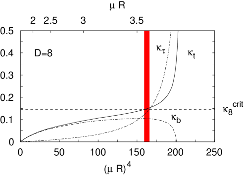
(b)

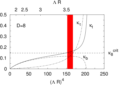
Figure 5: Binding strengths $\kappa_{t,b,\tau}$ with $D=8,n_{g}=1,R^{-1}=10$ TeV. The graphs (a) and (b) correspond with the $\overline{\rm MS}$- and PT-schemes, respectively. We also show $\kappa_{8}^{\rm crit}$ of Eq. (47) by the horizontal dashed line. The shaded region is the tMAC scale $\Lambda_{\rm tM}$ satisfying Eq. (41).

(a)

(b)

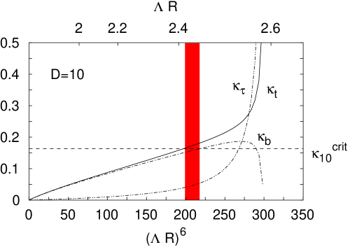
Figure 6: Binding strengths $\kappa_{t,b,\tau}$ with $D=10,n_{g}=1,R^{-1}=10$ TeV. The graphs (a) and (b) correspond with the $\overline{\rm MS}$- and PT-schemes, respectively. We also show $\kappa_{10}^{\rm crit}$ of Eq. (47) by the horizontal dashed line. The shaded region is the tMAC scale $\Lambda_{\rm tM}$ satisfying Eq. (41).

Now, we are ready to investigate the tMAC scale. We show behavior of the binding strengths $\kappa_{t,b,\tau}$ both in the $\overline{\rm MS}$- and PT-couplings in Figs. 4–6 to study the scheme dependence.

We first discuss the tMAC scale based on the $\overline{\rm MS}$-coupling. We compare attractive forces of top, bottom, and tau condensates with $\kappa_{D}^{\rm crit}$ in Figs. 4(a), 5(a) and 6(a) for $R^{-1}=10$ TeV. As the value of $\kappa_{D}^{\rm crit}$ becomes larger, the tMAC scale gets squeezed.

For $D=6$, we find that the tMAC scale is squeezed out, if we use the reference value $\kappa_{6}^{\rm crit}$ Eq. (47). The conclusion is unchanged against varying the compactification scale as far as $R^{-1}>1$ TeV. Actually, the tau condensation instead of the top condensation becomes the MAC. In order for the tMAC scale to survive, the value of $\kappa_{6}^{\rm crit}$ should be lower than the reference value by about 20% for $R^{-1}=$ 1–100 TeV, which is highly unlikely. Thus the scenario does not work for $D=6$.

For $D=8$, on the other hand, the tMAC scale $\Lambda_{\rm tM}$ satisfying Eq. (41) does exist,

$$\Lambda_{\rm tM}R=3.55\,\mbox{--}\,3.59,\quad(R^{-1}=\mbox{10 TeV}),$$ (49)

for the reference value of $\kappa_{D}^{\rm crit}$. If we vary the compactification scale as $R^{-1}=1$–100 TeV, we find the tMAC scale,

$$\Lambda_{\rm tM}R=3.5\,\mbox{--}\,3.6.$$ (50)

For $D=10$, the tMAC scale does not exist for $R^{-1}=10$ TeV. If we admit $R^{-1}\leq 5$ TeV, we barely find the tMAC scale $\Lambda_{\rm tM}R=2.56$–$2.57$ for $R^{-1}=1$–$5$ TeV.

We have studied the tMAC scale so far by using the $\overline{\rm MS}$-coupling. In order to clarify the scheme dependence, we also investigate the PT-coupling in the MAC analysis. We show binding strengths $\kappa_{t,b,\tau}$ in the PT-scheme in Figs. 4(b), 5(b) and 6(b) for $R^{-1}=10$ TeV. We find that the scheme dependence is negligibly small for $D=6$. Although behavior of the binding strengths $\kappa_{t,b,\tau}$ for $D=8$ somewhat depends on the regularization scheme, there does exist an overlapped region of the tMAC scale between the $\overline{\rm MS}$- and PT-schemes. For $D=10$, however, the scheme dependence is rather large: There is no overlap of the tMAC scale for $R^{-1}=1$–$100$ TeV.

In conclusion we have shown that the region of the tMAC scale is squeezed out for $D=6$, while the tMAC scale does exist for $D=8$ without much ambiguity. For $D=10$, we cannot obtain a reliable result because of the significant scheme dependence.

IV Prediction of $m_{t}$ and $m_{H}$

In this section, we calculate the top mass $m_{t}$ and the Higgs mass $m_{H}$ by using RGEs of the top Yukawa and Higgs quartic couplings with the compositeness conditions Bardeen:1989ds in a way used by ACDH Arkani-Hamed:2000hv .

Let us first recapitulate the compositeness conditions in Ref. Arkani-Hamed:2000hv : Assume that the top condensation takes place in the bulk. Then, at the compositeness scale $\Lambda$, a scalar bound state $H$ (composite Higgs),

$$H\sim(\bar{q}_{L}t_{R}),$$ (51)

is formed in the bulk, where $q_{L}[\equiv(t_{L},b_{L})^{T}]$ and $t_{R}$ are bulk fermions. At this stage, the composite Higgs $H$ does not propagate in the bulk. Its kinetic term is expected to develop at the scale below $\Lambda$. It is assumed that the effective theory below $\Lambda$ is described by the bulk SM. In the truncated KK effective theory of the bulk SM, the compositeness conditions then read

$$y(\mu)\to\infty,\quad\frac{\lambda(\mu)}{y(\mu)^{4}}\to 0,\quad(\mu\to\Lambda),$$ (52)

where $y$ and $\lambda$ denote the top Yukawa and Higgs quartic couplings, respectively.

We shall use the above procedure to calculate $m_{t}$ and $m_{H}$. In contrast to the ACDH analysis, however, we have shown existence of the tMAC scale for $D=8$ without much ambiguity and hence the extra dimension scenario of the TMSM is actually possible. Furthermore, while the compositeness scale $\Lambda$ in Ref. Arkani-Hamed:2000hv was treated as a free parameter to be adjusted for reproducing the experimental value of $m_{t}$, we identify the compositeness scale $\Lambda$ with the tMAC scale $\Lambda_{\rm tM}$,

$$\Lambda=\Lambda_{\rm tM},$$ (53)

which is no longer an adjustable parameter but constrained as Eq. (50). Thus we can test our model by comparing the predicted $m_{t}$ with the experimental value.

Within the truncated KK effective theory, RGEs for $y$ and $\lambda$ read 

$$(4\pi)^{2}\mu\frac{dy}{d\mu}=\beta_{y}^{\rm SM}+\beta_{y}^{\rm KK},$$ (54)

$$(4\pi)^{2}\mu\frac{d\lambda}{d\mu}=\beta_{\lambda}^{\rm SM}+\beta_{\lambda}^{\rm KK},$$ (55)

where

$$\beta_{y}^{\rm SM} = y\left[\,\left(3+\frac{3}{2}\right)y^{2}-8g_{3}^{2}-\frac{9}{4}g_{2}^{2}-\frac{17}{12}g_{Y}^{2}\,\right],$$ (56)

$$\beta_{y}^{\rm KK} = \left(6N_{\rm KK}^{f}+\frac{3}{2}N_{\rm KK}^{h}\right)\,y^{3}$$ (57)

$$\quad-N_{\rm KK}^{g}\left(8g_{3}^{2}+\frac{9}{4}g_{2}^{2}+\frac{17}{12}g_{Y}^{2}\right)\,y$$

$$\quad-\delta N_{\rm KK}^{gs}\left(\frac{4}{3}g_{3}^{2}-\frac{3}{8}g_{2}^{2}-\frac{1}{72}g_{Y}^{2}\right)\,y,$$

$$\beta_{\lambda}^{\rm SM} = 12\left(\lambda y^{2}-y^{4}\right)+12\lambda^{2}$$ (58)

$$\quad+\frac{3}{4}(3g_{2}^{4}+2g_{2}^{2}g_{Y}^{2}+g_{Y}^{4})$$

$$\quad-3(3g_{2}^{2}+g_{Y}^{2})\lambda,$$

$$\beta_{\lambda}^{\rm KK} = 24N_{\rm KK}^{f}\left(\lambda y^{2}-y^{4}\right)+12N_{\rm KK}^{h}\lambda^{2}$$ (59)

$$+N_{\rm KK}^{g}\left[\,\frac{3}{4}\left(3g_{2}^{4}+2g_{2}^{2}g_{Y}^{2}+g_{Y}^{4}\right)-3(3g_{2}^{2}+g_{Y}^{2})\lambda\,\right]$$

$$+\frac{\delta}{4}N_{\rm KK}^{gs}(3g_{2}^{4}+2g_{2}^{2}g_{Y}^{2}+g_{Y}^{4}).$$

Note that $\beta_{y,\lambda}^{\rm SM}$ and $\beta_{y,\lambda}^{\rm KK}$ stand for contributions of zero modes and KK modes, respectively. We calculate the RGEs by using the UV-BCs Eq. (52) and determine $m_{t}$ and $m_{H}$ through the conditions,

$$m_{t}=\frac{v}{\sqrt{2}}\,y(m_{t}),\quad m_{H}=v\sqrt{\lambda(m_{H})},$$ (60)

with $v=246$ GeV.

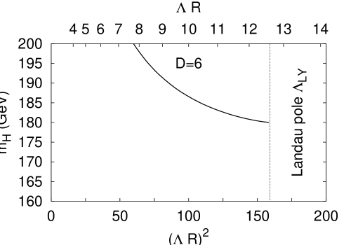
Figure 7: Solutions $m_{t}$ and $m_{H}$ of Eq. (60) with the compositeness conditions (52) for $D=6,R^{-1}=10$ TeV. The dashed vertical line represents the Landau pole $\Lambda_{LY}$.

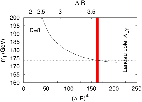
Figure 8: Solutions $m_{t}$ and $m_{H}$ of Eq. (60) with the compositeness conditions (52) for $D=8,R^{-1}=10$ TeV. The dashed vertical line represents the Landau pole $\Lambda_{LY}$. The shaded region is the tMAC scale $\Lambda_{\rm tM}$ satisfying Eq. (41).

Figure 9: Solutions $m_{t}$ and $m_{H}$ of Eq. (60) with the compositeness conditions (52) for $D=10,R^{-1}=10$ TeV. The dashed vertical line represents the Landau pole $\Lambda_{LY}$.

We show results of $m_{t}$ and $m_{H}$ in Figs. 7, 8, 9 for $D=6,8,10$, $R^{-1}=10$ TeV for various values of the compositeness scale $\Lambda$. As we have shown in Sec. III, the tMAC scale does exist only for $D=8$ without much ambiguity, $\Lambda_{\rm tM}R=3.5$–$3.6$. Identifying $\Lambda$ with $\Lambda_{\rm tM}$, we depict the region of the tMAC scale for $D=8$ by the shaded area in Fig. 8. There is no shaded region in Figs. 7 and 9, because a sensible tMAC scale is absent for $D=6,10$. For $D=8$ we predict

$$m_{t}=172-175\;\mbox{GeV},$$ (61)

and

$$m_{H}=176-188\;\mbox{GeV},$$ (62)

for the range of the compactification scale $R^{-1}=$ 1–100 TeV. The uncertainties in Eqs. (61) and (62) also include error of $\alpha_{3}(M_{Z})=0.1172\pm 0.0020$ PDG .

Remarkably, the prediction Eq. (61) for $m_{t}$ is consistent with the reality, the $\overline{\rm MS}$-mass $m_{t}=164.7\pm 4.9$ GeV which is calculated from the observed value of the pole mass, $174.3\pm 5.1$ GeV PDG . It should be emphasized that the compositeness scale $\Lambda$ in Ref. Arkani-Hamed:2000hv is an arbitrary parameter and was adjusted to reproduce the experimental value of the top mass. On the contrary, our compositeness scale $\Lambda$ is fixed by the tMAC scale $\Lambda_{\rm tM}$ by requiring that the top quark condensation actually takes place, while other condensations do not. Hence the top mass as well as the Higgs mass is the prediction in our approach.

Compared with the prediction of Ref. Arkani-Hamed:2000hv , $m_{H}\sim 170-230$ GeV for $D=8$, Eq. (62) is determined more sharply. This is because our compositeness scale $\Lambda$ is given by the tMAC scale $\Lambda_{\rm tM}$ which is more severely constrained than $\Lambda$ of Ref. Arkani-Hamed:2000hv , the value determined from the top mass within 3$\sigma$ of the experimental value.

We now discuss the reason why the value of Eq. (61) is significantly smaller than that of the original TMSM in four dimensions which predicted $m_{t}\gtrsim 200$ GeV. Let us consider a simplified RGE for $y$ neglecting the electroweak gauge interactions:

$$(4\pi)^{2}\mu\frac{dy}{d\mu} = \left(2N_{c}N_{\rm KK}^{f}+\frac{3}{2}N_{\rm KK}^{h}\right)\,y^{3}$$ (63)

$$-(6N_{\rm KK}^{g}+\delta N_{\rm KK}^{gs})\,C_{F}\,y\,g_{3}^{2},$$

with $N_{c}=3$, $C_{F}=4/3$. Using Eq. (14) as an approximation for $N_{\rm KK}^{i}$ and equating the R.H.S. of Eq. (63) to zero, we find the quasi IR fixed point $y_{\rm qIR}(\mu)$ Hill:1980sq

$$y_{\rm qIR}(\mu)=g_{3}(\mu)\cdot\sqrt{\frac{C_{F}(6+\delta)}{2^{\delta/2}N_{c}+\frac{3}{2}}}.$$ (64)

The value of Eq. (64) decreases as $\delta(\equiv D-4)$ increases at $\mu=R^{-1}$, since the value of $g_{3}(R^{-1})$ is determined within the SM independently of $\delta$. In the original TMSM with $D=4$ the prediction of $m_{t}$ is governed by Eq. (64) with $\delta=0$ Bardeen:1989ds . As a result, the prediction of $m_{t}$ with $\delta>0$ is substantially lower than that of the original TMSM with $\delta=0$.

The mechanism is still operative even including the electroweak gauge interactions: In Fig. 10, we show the quasi IR fixed point and the behavior of $y$ based on the full one-loop RGE (54) with various boundary conditions at $\Lambda$. We also show the Pendleton-Ross (PR) fixed point Pendleton:as determined from $\frac{d}{d\mu}\frac{y}{g_{3}}=0$:

$$y_{\rm PR}(\mu)=g_{3}(\mu)\cdot\sqrt{\frac{(6+\delta)C_{F}+b^{\prime}_{3}}{2^{\delta/2}N_{c}+\frac{3}{2}}}$$ (65)

with $b^{\prime}_{3}$ being

$$b^{\prime}_{3}=\left(-\frac{11}{3}+\frac{\delta}{6}\right)C_{A}+\frac{8}{3}\cdot 2^{\delta/2}T_{R}$$ (66)

and $C_{A}=N_{c}$, $T_{R}=1/2$. For $b^{\prime}_{3}=0$ the PR fixed point is identical to the quasi IR fixed point. As far as $b^{\prime}_{3}<0$ $(D=6,8)$, the value of the PR fixed point is smaller than that of the quasi IR fixed point, $y_{\rm PR}<y_{\rm qIR}$, while $y_{\rm PR}>y_{\rm qIR}$ for $D=10$. The top Yukawa coupling at $R^{-1}$ for $D=6,8$ is actually between $y_{\rm PR}$ and $y_{\rm qIR}$ for a sufficiently large top Yukawa, $y(\Lambda)\gtrsim 1$, at high energy scale $(\Lambda R)^{\delta}\gg 1$. We note here that the actual prediction of $m_{t}$ with $D=6,8$ is even smaller than the value expected from $y_{\rm qIR}$.

We also comment that the predicted values of $m_{t}$ and $m_{H}$ would be stable thanks to these fixed points, even if the estimate of the tMAC scale were somewhat changed from ours for some reason.

As was already pointed out in Ref. Arkani-Hamed:2000hv , the lower value prediction of $m_{t}$ than that of the original TMSM can also be understood as follows: Since KK modes of the top quark ($t^{(n)}$) as well as its zero mode ($t^{(0)}$) contribute to the VEV $v$,

$$v\,\propto\,\langle\bar{t}^{(0)}t^{(0)}\rangle+\sum_{n>0}\langle\bar{t}^{(n)}t^{(n)}\rangle,$$ (67)

the condensate $\langle\bar{t}^{(0)}t^{(0)}\rangle$ is suppressed compared with the original TMSM and so is the top mass.

Now we discuss implication of our Higgs mass prediction Eq. (62). The upper limit of $m_{H}$ from radiative corrections in the SM is $m_{H}<199$ GeV at 95% CL PDG . The prediction Eq. (62) is still below this upper limit. In order to discriminate the present model from the SM in experiments, we need further information of physics at the compactification scale. However, the Higgs boson in such a mass range, $m_{H}=176-188$ GeV, is characteristically small within the framework of the dynamical EWSB. Yet the value is substantially larger than that of typical supersymmetric models, $m_{H}\mathop{<}\limits_{\displaystyle{\sim}}130$ GeV. Thus the present scenario is clearly distinguished from most of the models beyond the SM simply through the Higgs mass observation. The Higgs boson of this mass range decays into weak boson pair almost 100%. It will be immediately discovered in $H\to WW^{(*)}/ZZ^{(*)}$ once the LHC starts.

Figure 10: RGE flows for the top Yukawa coupling $y$. We also show the quasi IR fixed point $y_{\rm qIR}$ and the PR fixed point $y_{\rm PR}$ at $\mu=R^{-1}$. The graphs from top to bottom represent running of $y$ for $D=6,8,10$, respectively. $R^{-1}=10$ TeV was assumed. We used the full one-loop RGE (54). The UV-BCs are $y(\Lambda)\to\infty$ (solid lines) and $y(\Lambda)=\sqrt{2}$ (dashed and dash-dotted lines) for two typical values of $\Lambda$.

V Summary and discussions

We have argued a viable top mode standard model (TMSM) with TeV-scale extra dimensions where bulk $SU(3)\times SU(2)\times U(1)$ SM gauge interactions (without ad hoc four-fermion interactions) trigger condensate of only the top quark, but not of other quarks and leptons. In order for such a situation to be realized, the binding strength $\kappa$ should exceed the critical binding strength $\kappa_{D}^{\rm crit}$ only for the top quark (tMAC),

$$\kappa_{t}(\Lambda_{\rm tM})>\kappa_{D}^{\rm crit}>\kappa_{b}(\Lambda_{\rm tM}),\kappa_{\tau}(\Lambda_{\rm tM}),\cdots.$$ (68)

The binding strengths $\kappa_{t,b,\tau}$ were calculated by using RGEs for bulk SM gauge couplings. Comparing $\kappa_{t,b,\tau}$ with $\kappa_{D}^{\rm crit}$, we searched for the region of the tMAC scale $\Lambda_{\rm tM}$ satisfying Eq. (68). We then found that the region of the tMAC scale is squeezed out for $D=6$ for the reference value of $\kappa_{D}^{\rm crit}$ in Ref. Hashimoto:2000uk , while it does exist for $D=8$, $\Lambda_{\rm tM}=$ (3.5–3.6)$R^{-1}$. We were not able to draw a reliable conclusion for $D=10$, since the MAC analysis for $D=10$ strongly depends on the regularization scheme.

For $D=8$, we predicted the top mass $m_{t}$ and the Higgs mass $m_{H}$:

$$m_{t}=172-175\;\mbox{GeV}$$ (69)

and

$$m_{H}=176-188\;\mbox{GeV},$$ (70)

by using RGEs for the top Yukawa and Higgs quartic couplings with the compositeness conditions at the tMAC scale $\Lambda_{\rm tM}$. Our predictions are governed by the quasi IR-FP and hence are stable against varying the composite scale. The predicted values would not be changed so much, even if the region of the tMAC scale got wider than our estimate for some reason.

Why is the value of Eq. (69) significantly smaller than that of the original TMSM in four dimensions which predicted $m_{t}\gtrsim 200$ GeV? The value of the top Yukawa coupling at the quasi IR-FP is $y\simeq g_{3}\cdot\sqrt{C_{F}(6+\delta)/(2^{\delta/2}N_{c}+3/2)}$. Thanks to the suppression factor $2^{-\delta/2}$ in $y$, the mass of the top quark decreases as the number of dimensions increases.

The predicted Higgs mass Eq. (70) is substantially larger than that of typical supersymmetric models, while it is distinctively small as a dynamical EWSB scenario. We are thus able to distinguish the present model from typical supersymmetric or dynamical EWSB scenarios simply through the Higgs mass observation. We also note that the Higgs boson in this mass range will be immediately discovered in $H\to WW^{(*)}/ZZ^{(*)}$ once the LHC starts. The upper limit of $m_{H}$ from radiative corrections in the SM is $m_{H}<199$ GeV at 95% CL PDG and the predicted value Eq. (70) is below this upper limit, however. It is thus difficult to discriminate the Higgs in the present model from that of the SM only from its mass. We definitely need experimental information other than $m_{H}$ in order to establish the present model.

Many issues remain to be explored:

1) Our results on the tMAC scale are sensitive to the value of $\kappa_{D}^{\rm crit}$. Although we used the reference value of $\kappa_{D}^{\rm crit}$ in the approach of the ladder SD equation neglecting the effect of the compactification, it would be more preferable if we can determine $\kappa_{D}^{\rm crit}$ more reliably. For such a purpose, we should take into account effects of the compactification scale $R^{-1}$ which turned out not so small compared with the tMAC scale $\Lambda_{\rm tM}$ in our analysis. We also need running of bulk gauge couplings beyond one-loop perturbation.

2) We incorporated only one composite Higgs doublet into RGEs, assuming other possible bound states such as vector/axial-vector bosons are irrelevant. In order to justify the assumption, we need to solve bound state problems in the bulk gauge theories. Once such a composite scalar exists, it should be a tightly bound state formed by strong short distance dynamics with large anomalous dimension. Such a system is expected to resemble the gauged Nambu-Jona-Lasinio (GNJL) model where the compositeness condition is explicitly formulated. Actually, as it happened in the 4-dimensional case Bardeen:sm ; Kondo-Shuto-Yamawaki ; Aokietal , the pure gauge dynamics strong at short distance in our case can also induce strong four-fermion interactions which may become relevant operators due to large anomalous dimensions, $\gamma_{m}\sim D/2-1$ Hashimoto:2000uk . We will report elsewhere the phase structure of the bulk GNJL model future .

3) There are potential constraints on our model from precision electroweak measurements. The summation of KK modes below the cutoff $\Lambda$ contributes to $\Delta\rho$ as $\Delta\rho\sim(\Lambda R)^{D-6}(M_{W}R)^{2}$ Nath:1999fs . In our case with $\Lambda=\Lambda_{\rm tM}$, $(\Lambda_{\rm tM}R)^{D-6}\sim 10$ for $D=8$, we thus need to take $R^{-1}\gtrsim{\cal O}(\mbox{10 TeV})$, which may be subtle about the fine tuning. More involved estimate will be done elsewhere.

4) Masses of other quarks and leptons have not been dealt with in this paper. In the original TMSM, these masses are descended from the top condensate through ad hoc flavor-breaking four-fermion interactions MTY89 . The origin of such four-fermion interactions will be highly hoped for in the present scenario.

5) Our scenario crucially relies on the short distance strong dynamics around the composite scale. We thus need a better-controlled theory in the UV-region. It would be interesting to study a deconstructed/latticized version Arkani-Hamed:2001ca of our model.

Appendix A Counting of $N_{\rm KK}$

The torus compactification of extra dimensions leaves vector-like zero-modes in the 4-dimensional space-time, even if we start with a chiral gauge theory in the bulk. We thus need to compactify the extra dimensions to an orbifold in order to obtain the conventional SM particles as zero modes. An example of such a compactification was explicitly constructed in Ref.Hashimoto:2000uk based on the $T^{\delta}/Z_{2}^{\delta/2}$ orbifold for $D=4+\delta$ ($\delta=$ even) dimensions. In this Appendix, we discuss the massive KK spectrum in the orbifold compactification of Ref.Hashimoto:2000uk .

A.1 $D=4+2$

Let us start with the 6-dimensional case ($D=4+\delta$, $\delta=2$). The 6-dimensional space-time is decomposed into conventional and extra dimensions,

$$x^{M}=(x^{\mu},y^{m})$$ (71)

with $M=0,1,2,3,5,6$, $\mu=0,1,2,3$ and $m=5,6$. We assume the compactification radius $R$ and the fields at $(x^{\mu},y^{5}+2\pi R,y^{6})$ and $(x^{\mu},y^{5},y^{6}+2\pi R)$ are identified with the field at $(x^{\mu},y^{5},y^{6})$. We thus impose the periodic boundary conditions,

$$A^{M}(x,y^{5},y^{6}) = A^{M}(x,y^{5}+2\pi R,y^{6})$$ (72a)

$$= A^{M}(x,y^{5},y^{6}+2\pi R),$$

for a gauge field and

$$\psi(x,y^{5},y^{6}) = \psi(x,y^{5}+2\pi R,y^{6})$$ (72b)

$$= \psi(x,y^{5},y^{6}+2\pi R)$$

for a fermion.

The $Z_{2}$ identification of the orbifold $T^{2}/Z_{2}$ leads to the orbifold boundary conditions (BCs),

$$A^{\mu}(x,y)=A^{\mu}(x,-y) \mbox{for $\mu=0,1,2,3$},$$ (73a)

$$A^{m}(x,y)=-A^{m}(x,-y) \mbox{for $m=5,6$},$$ (73b)

$$\psi(x,y)=\Gamma_{A,5}\Gamma_{A,7}\psi(x,-y).$$ (73c)

Here $\Gamma_{A,5}$ and $\Gamma_{A,7}$ are chirality matrices in four- and six-dimensions, respectively,

$$\Gamma_{A,5}\equiv i\Gamma^{0}\Gamma^{1}\Gamma^{2}\Gamma^{3},\quad\Gamma_{A,7}\equiv-\Gamma^{0}\Gamma^{1}\Gamma^{2}\Gamma^{3}\Gamma^{5}\Gamma^{6}.$$ (74)

It is easy to show that the gauge-vector field $A_{\mu}$ is decomposed into its KK-modes,

$$A_{\mu}(x,y)=A_{\mu,00}(x)$$ (75)

$$+\sum_{n_{1}>0}A_{\mu,c0}^{[n_{1}]}\cos\left(\dfrac{n_{1}y^{5}}{R}\right)$$

$$+\sum_{n_{1}>0}A_{\mu,0c}^{[n_{1}]}\cos\left(\dfrac{n_{1}y^{6}}{R}\right)$$

$$+\sum_{n_{1},n_{2}>0}A_{\mu,cc}^{[n_{1},n_{2}]}\cos\left(\dfrac{n_{1}y^{5}}{R}\right)\cos\left(\dfrac{n_{2}y^{6}}{R}\right)$$

$$+\sum_{n_{1},n_{2}>0}A_{\mu,ss}^{[n_{1},n_{2}]}\sin\left(\dfrac{n_{1}y^{5}}{R}\right)\sin\left(\dfrac{n_{2}y^{6}}{R}\right),$$

with $n_{1}$, $n_{2}$ being positive integers, where we omitted the arguments for the KK-modes at $x^{\mu}$, except for the zero mode $A_{\mu,00}$. We note that the orbifold condition Eq.(73a) leads to

$$A_{\mu,0s}^{[n_{1}]}=A_{\mu,s0}^{[n_{1}]}=A_{\mu,cs}^{[n_{1},n_{2}]}=A_{\mu,sc}^{[n_{1},n_{2}]}=0$$ (76)

in the KK-spectrum. In order to investigate the KK-spectrum, we define sets of the KK-fields,

$${\cal A}_{\mu}^{\delta=2,[n_{1}]} \equiv \{A_{\mu,c0}^{[n_{1}]}(x),\,A_{\mu,0c}^{[n_{1}]}(x)\},$$ (77a)

$${\cal A}_{\mu}^{\delta=2,[n_{1},n_{2}]} \equiv \{A_{\mu,cc}^{[n_{1},n_{2}]}(x),\,A_{\mu,ss}^{[n_{1},n_{2}]}(x)\}.$$ (77b)

The masses of these KK-states are given by $m_{n_{1}}^{2}=n_{1}^{2}R^{-2}$ for a state contained in ${\cal A}_{\mu}^{2,[n_{1}]}$ and $m_{\vec{n}}^{2}=(n_{1}^{2}+n_{2}^{2})R^{-2}$ for ${\cal A}_{\mu}^{2,[n_{1},n_{2}]}$. Using the number of elements of these sets,

$${\cal N}_{g}^{\delta=2,[n_{1}]}={\cal N}_{g}^{\delta=2,[n_{1},n_{2}]}=2,$$ (78)

the number of KK-modes of gauge bosons $A_{\mu}$ with $m_{\vec{n}}^{2}\leq\mu^{2}$ is written as

$$N_{\rm KK}^{g}(\mu;\delta=2)=$$ (79)

$${\cal N}_{g}^{\delta=2,[n_{1}]}\cdot N_{1}(\mu)+{\cal N}_{g}^{\delta=2,[n_{1},n_{2}]}\cdot N_{2}(\mu)$$

for $D=4+2$ dimensions, where $N_{1}(\mu)$ and $N_{2}(\mu)$ are given by

$$N_{1}(\mu)\equiv\sum_{n_{1}>0}^{n_{1}^{2}\leq\mu^{2}R^{2}}1,\quad N_{2}(\mu)\equiv\sum_{n_{1},n_{2}>0}^{n_{1}^{2}+n_{2}^{2}\leq\mu^{2}R^{2}}1,$$ (80)

respectively.

It is straightforward to perform similar analysis for the gauge scalar $A_{m}$. Since the zero-mode of $A_{m}$ is projected out from the KK-spectrum due to the orbifold BC (73b), the KK decomposition of $A_{m}$ is given by

$$A_{m}(x,y)=$$ (81)

$$\sum_{n_{1}>0}A_{m,s0}^{[n_{1}]}\sin\left(\dfrac{n_{1}y^{5}}{R}\right)$$

$$+\sum_{n_{1}>0}A_{m,0s}^{[n_{1}]}\sin\left(\dfrac{n_{1}y^{6}}{R}\right)$$

$$+\sum_{n_{1},n_{2}>0}A_{m,cs}^{[n_{1},n_{2}]}\cos\left(\dfrac{n_{1}y^{5}}{R}\right)\sin\left(\dfrac{n_{2}y^{6}}{R}\right)$$

$$+\sum_{n_{1},n_{2}>0}A_{m,sc}^{[n_{1},n_{2}]}\sin\left(\dfrac{n_{1}y^{5}}{R}\right)\cos\left(\dfrac{n_{2}y^{6}}{R}\right).$$

Sets of the KK-fields are defined as

$${\cal A}_{m}^{\delta=2,[n_{1}]} \equiv \{A_{m,s0}^{[n_{1}]}(x),\,A_{m,0s}^{[n_{1}]}(x)\},$$ (82a)

$${\cal A}_{m}^{\delta=2,[n_{1},n_{2}]} \equiv \{A_{m,cs}^{[n_{1},n_{2}]}(x),\,A_{m,sc}^{[n_{1},n_{2}]}(x)\}$$ (82b)

in a similar manner to Eqs.(77), where the number of elements are given by

$${\cal N}_{gs}^{\delta=2,[n_{1}]}={\cal N}_{gs}^{\delta=2,[n_{1},n_{2}]}=2.$$ (83)

We can now easily count the number of KK-modes of the gauge scalars $A_{m}$,

$$N_{\rm KK}^{gs}(\mu;\delta=2)=$$ (84)

$${\cal N}_{gs}^{\delta=2,[n_{1}]}\cdot N_{1}(\mu)+{\cal N}_{gs}^{\delta=2,[n_{1},n_{2}]}\cdot N_{2}(\mu).$$

We next consider the KK spectrum of the bulk chiral fermion $\psi_{+}(x,y)$,

$$\Gamma_{A,7}\psi_{+}(x,y)=+\psi_{+}(x,y),$$ (85)

in $D=4+2$ dimensions, which has obviously 4-components. The orbifold BC (73c) reads

$$\psi_{+}(x,y)=+\Gamma_{A,5}\psi_{+}(x,-y).$$ (86)

The KK expansion of $\psi_{+}$ is thus given by

$$\psi_{+}(x,y)=\psi_{+,00}(x)$$

$$+\sum_{n_{1}>0}\psi_{+,c0}^{[n_{1}]}(x)\cos\left(\dfrac{n_{1}y^{5}}{R}\right)$$

$$+\sum_{n_{1}>0}\psi_{+,0c}^{[n_{1}]}(x)\cos\left(\dfrac{n_{1}y^{6}}{R}\right)$$

$$+\sum_{n_{1},n_{2}>0}\psi_{+,cc}^{[n_{1},n_{2}]}(x)\cos\left(\dfrac{n_{1}y^{5}}{R}\right)\cos\left(\dfrac{n_{2}y^{6}}{R}\right)$$

$$+\sum_{n_{1},n_{2}>0}\psi_{+,ss}^{[n_{1},n_{2}]}(x)\sin\left(\dfrac{n_{1}y^{5}}{R}\right)\sin\left(\dfrac{n_{2}y^{6}}{R}\right)$$

$$+\sum_{n_{1}>0}\psi_{+,s0}^{[n_{1}]}(x)\sin\left(\dfrac{n_{1}y^{5}}{R}\right)$$

$$+\sum_{n_{1}>0}\psi_{+,0s}^{[n_{1}]}(x)\sin\left(\dfrac{n_{1}y^{6}}{R}\right)$$

$$+\sum_{n_{1},n_{2}>0}\psi_{+,cs}^{[n_{1},n_{2}]}(x)\cos\left(\dfrac{n_{1}y^{5}}{R}\right)\sin\left(\dfrac{n_{2}y^{6}}{R}\right)$$

$$+\sum_{n_{1},n_{2}>0}\psi_{+,sc}^{[n_{1},n_{2}]}(x)\sin\left(\dfrac{n_{1}y^{5}}{R}\right)\cos\left(\dfrac{n_{2}y^{6}}{R}\right)$$

with 2-component fermions. In particular, we find that the zero-mode is right-handed under the 4-dimensional chiral rotation, thanks to Eq.(73c),

$$\Gamma_{A,5}\psi_{+,00}(x)=+\psi_{+,00}(x).$$ (88)

Other KK modes include both of right, and left-handed fermions. We thus define sets of KK-fields,

$$\psi_{+,R}^{\delta=2,[n_{1}]} \equiv \{\psi_{+,c0}^{[n_{1}]}(x),\,\psi_{+,0c}^{[n_{1}]}(x)\},$$ (89a)

$$\psi_{+,R}^{\delta=2,[n_{1},n_{2}]} \equiv \{\psi_{+,cc}^{[n_{1},n_{2}]}(x),\,\psi_{+,ss}^{[n_{1},n_{2}]}(x)\},$$ (89b)

$$\psi_{+,L}^{\delta=2,[n_{1}]} \equiv \{\psi_{+,s0}^{[n_{1}]}(x),\,\psi_{+,0s}^{[n_{1}]}(x)\},$$ (89c)

$$\psi_{+,L}^{\delta=2,[n_{1},n_{2}]} \equiv \{\psi_{+,cs}^{[n_{1},n_{2}]}(x),\,\psi_{+,sc}^{[n_{1},n_{2}]}(x)\}.$$ (89d)

The KK fields in $\psi_{+,R}^{2,[n_{1}]}$ and $\psi_{+,R}^{2,[n_{1},n_{2}]}$ ($\psi_{+,L}^{2,[n_{1}]}$ and $\psi_{+,L}^{2,[n_{1},n_{2}]}$) are right-handed (left-handed). These KK-modes acquire their Dirac masses among $\psi_{+,R}^{2,[n_{1}]}$ and $\psi_{+,L}^{2,[n_{1}]}$ ($\psi_{+,R}^{2,[n_{1},n_{2}]}$ and $\psi_{+,L}^{2,[n_{1},n_{2}]}$) in four dimensions. The number of these KK Dirac fermions is therefore given by

$$N_{\rm KK}^{f}(\mu;\delta=2)=$$ (90)

$${\cal N}_{f}^{\delta=2,[n_{1}]}\cdot N_{1}(\mu)+{\cal N}_{f}^{\delta=2,[n_{1},n_{2}]}\cdot N_{2}(\mu)$$

with

$${\cal N}_{f}^{\delta=2,[n_{1}]} \equiv \#\psi_{+,R}^{2,[n_{1}]}$$ (91a)

$$= \#\psi_{+,L}^{2,[n_{1}]}=2,$$

$${\cal N}_{f}^{\delta=2,[n_{1},n_{2}]} \equiv \#\psi_{+,R}^{2,[n_{1},n_{2}]}$$ (91b)

$$= \#\psi_{+,L}^{2,[n_{1},n_{2}]}=2.$$

We note

$$N_{\rm KK}^{g}(\mu;\delta=2)=N_{\rm KK}^{gs}(\mu;\delta=2)=N_{\rm KK}^{f}(\mu;\delta=2)$$ (92)

for $D=4+2$ dimensions.

It is straightforward to apply the above procedure to the bulk chiral fermion $\psi_{-}(x,y)$,

$$\Gamma_{A,7}\psi_{-}(x,y)=-\psi_{-}(x,y).$$ (93)

We easily find that the zero mode of $\psi_{-}(x,y)$ is left-handed. We thus identify the right[left]-handed fermions in the SM to $\psi_{+}(x,y)$ [$\psi_{-}(x,y)$]. The number of the KK Dirac fermions for $\psi_{-}$ is equal to Eq. (90).

For the (composite) Higgs field, we take the same $Z_{2}$ identification as Eq. (73a). This always leads to

$$N_{\rm KK}^{h}(\mu;\delta)=N_{\rm KK}^{g}(\mu;\delta)$$ (94)

for the number of KK modes of the Higgs field. Hereafter, we abbreviate $\delta$ in the arguments of $N_{\rm KK}^{i}(\mu;\delta)$, $(i=g,gs,f,h)$, when the number of $\delta$ is obvious.

A.2 $D=4+4$

Let us next turn to the 8-dimensional case ($D=4+\delta$, $\delta=4$),

$$x^{M}=(x^{\mu},y^{m},z^{m^{\prime}}),\quad m=5,6,\quad m^{\prime}=7,8.$$ (95)

We impose the orbifold BCs:

$$A^{\mu}(x,y,z) = A^{\mu}(x,-y,z)$$ (96a)

$$= A^{\mu}(x,y,-z),$$

$$A^{m}(x,y,z) = -A^{m}(x,-y,z)$$ (96b)

$$= A^{m}(x,y,-z),$$

$$A^{m^{\prime}}(x,y,z) = A^{m^{\prime}}(x,-y,z)$$ (96c)

$$= -A^{m^{\prime}}(x,y,-z),$$

and

$$\psi(x,y,z) = \Gamma_{A,7^{\prime}}\Gamma_{A,9}\psi(x,-y,z)$$ (96d)

$$= \Gamma_{A,7}\Gamma_{A,9}\psi(x,y,-z),$$

with

$$\Gamma_{A,7^{\prime}} = -\Gamma^{0}\Gamma^{1}\Gamma^{2}\Gamma^{3}\Gamma^{7}\Gamma^{8}$$

$$\Gamma_{A,9} = -i\Gamma^{0}\Gamma^{1}\Gamma^{2}\Gamma^{3}\Gamma^{5}\Gamma^{6}\Gamma^{7}\Gamma^{8}.$$ (97)

Noting the relations,

$$\Gamma_{A,7^{\prime}}\Gamma_{A,9}=\Gamma_{A,5}\Gamma_{A,7},\quad\Gamma_{A,7}\Gamma_{A,9}=\Gamma_{A,5}\Gamma_{A,7^{\prime}},$$ (98)

we can easily see that the zero-mode of the 8-dimensional bulk chiral fermion $\psi_{+}$ is chiral under the 4-dimensional chiral symmetry.

The bulk gauge field is decomposed into its KK-modes in a similar manner with the $D=4+2$ case. We obtain

$${\cal A}_{\mu}^{\delta=4,[n]_{1}}=$$ (99a)

$$\{A_{\mu,c000}^{[n]_{1}},\,A_{\mu,0c00}^{[n]_{1}},\,A_{\mu,00c0}^{[n]_{1}},\,A_{\mu,000c}^{[n]_{1}}\},$$

$${\cal A}_{\mu}^{\delta=4,[n]_{2}}=$$ (99b)

$$\{A_{\mu,cc00}^{[n]_{2}},\,A_{\mu,00cc}^{[n]_{2}},\,A_{\mu,ss00}^{[n]_{2}},\,A_{\mu,00ss}^{[n]_{2}},\,$$

$$\quad A_{\mu,c0c0}^{[n]_{2}},\,A_{\mu,c00c}^{[n]_{2}},\,A_{\mu,0cc0}^{[n]_{2}},\,A_{\mu,0c0c}^{[n]_{2}}\},$$

$${\cal A}_{\mu}^{\delta=4,[n]_{3}}=$$ (99c)

$$\{A_{\mu,ccc0}^{[n]_{3}},\,A_{\mu,cc0c}^{[n]_{3}},\,A_{\mu,c0cc}^{[n]_{3}},\,A_{\mu,0ccc}^{[n]_{3}},\,$$

$$\quad A_{\mu,ssc0}^{[n]_{3}},\,A_{\mu,ss0c}^{[n]_{3}},\,A_{\mu,c0ss}^{[n]_{3}},\,A_{\mu,0css}^{[n]_{3}}\},$$

$${\cal A}_{\mu}^{\delta=4,[n]_{4}}=$$ (99d)

$$\{A_{\mu,cccc}^{[n]_{4}},\,A_{\mu,ccss}^{[n]_{4}},\,A_{\mu,sscc}^{[n]_{4}},\,A_{\mu,ssss}^{[n]_{4}}\},$$

for the KK-expansion of $A_{\mu}$. Here $[n]_{i}$ stands for

$$[n]_{1}\equiv[n_{1}],\quad[n]_{2}\equiv[n_{1},n_{2}],\quad[n]_{3}\equiv[n_{1},n_{2},n_{3}],\cdots.$$ (100)

We thus find

$${\cal N}_{g}^{\delta=4,[n]_{1}} = 4,\quad{\cal N}_{g}^{\delta=4,[n]_{2}}=8,$$ (101a)

$${\cal N}_{g}^{\delta=4,[n]_{3}} = 8,\quad{\cal N}_{g}^{\delta=4,[n]_{4}}=4.$$ (101b)

For $A_{m}$ ($m=5,6$) we obtain

$${\cal A}_{m}^{\delta=4,[n]_{1}}=$$ (102a)

$$\{A_{m,s000}^{[n]_{1}},\,A_{m,0s00}^{[n]_{1}}\},$$

$${\cal A}_{m}^{\delta=4,[n]_{2}}=$$ (102b)

$$\{A_{m,sc00}^{[n]_{2}},\,A_{m,cs00}^{[n]_{2}},\,A_{m,s0c0}^{[n]_{2}},\,A_{m,s00c}^{[n]_{2}},\,$$

$$\quad A_{m,0sc0}^{[n]_{2}},\,A_{\mu,0s0c}^{[n]_{2}}\},$$

$${\cal A}_{m}^{\delta=4,[n]_{3}}=$$ (102c)

$$\{A_{m,scc0}^{[n]_{3}},\,A_{m,sc0c}^{[n]_{3}},\,A_{m,csc0}^{[n]_{3}},\,A_{m,cs0c}^{[n]_{3}},\,$$

$$\quad A_{m,s0cc}^{[n]_{3}},\,A_{m,0scc}^{[n]_{3}},\,A_{m,s0ss}^{[n]_{3}},\,A_{m,0sss}^{[n]_{3}}\},$$

$${\cal A}_{m}^{\delta=4,[n]_{4}}=$$ (102d)

$$\{A_{m,sccc}^{[n]_{4}},\,A_{m,cscc}^{[n]_{4}},\,A_{m,scss}^{[n]_{4}},\,A_{m,csss}^{[n]_{4}}\}.$$

It is straightforward to obtain similar expression for $A_{m^{\prime}}$ ($m^{\prime}=7,8$). We find

$${\cal N}_{gs}^{\delta=4,[n]_{1}} = 2,\quad{\cal N}_{gs}^{\delta=4,[n]_{2}}=6,$$ (103a)

$${\cal N}_{gs}^{\delta=4,[n]_{3}} = 8,\quad{\cal N}_{gs}^{\delta=4,[n]_{4}}=4.$$ (103b)

The numbers of KK-modes of gauge fields and gauge scalars are given by

$$N_{\rm KK}^{g}(\mu;\delta=4) = \sum_{k=1}^{4}{\cal N}_{g}^{4,[n]_{k}}\cdot N_{k}(\mu),$$ (104a)

$$N_{\rm KK}^{gs}(\mu;\delta=4) = \sum_{k=1}^{4}{\cal N}_{gs}^{4,[n]_{k}}\cdot N_{k}(\mu),$$ (104b)

where $N_{k}(\mu)$’s are defined in Eq.(80) for $k=1,2$ and

$$N_{3}(\mu) \equiv \sum_{n_{1},n_{2},n_{3}>0}^{n_{1}^{2}+n_{2}^{2}+n_{3}^{2}\leq\mu^{2}R^{2}}1,$$

$$N_{4}(\mu) \equiv \sum_{n_{1},n_{2},n_{3},n_{4}>0}^{n_{1}^{2}+n_{2}^{2}+n_{3}^{2}+n_{4}^{2}\leq\mu^{2}R^{2}}1$$ (105)

for $k=3,4$.

For a bulk chiral fermion $\psi_{+}$ in $D=4+\delta$ ($\delta=4$) dimensions, we find

$${\cal N}_{f}^{\delta=4,[n]_{1}} \equiv \#\psi_{+,R}^{4,[n]_{1}}$$ (106a)

$$= \#\psi_{+,L}^{4,[n]_{1}}=4,$$

$${\cal N}_{f}^{\delta=4,[n]_{2}} \equiv \#\psi_{+,R}^{4,[n]_{2}}$$ (106b)

$$= \#\psi_{+,L}^{4,[n]_{2}}=12,$$

$${\cal N}_{f}^{\delta=4,[n]_{3}} \equiv \#\psi_{+,R}^{4,[n]_{3}}$$ (106c)

$$= \#\psi_{+,L}^{4,[n]_{3}}=16,$$

$${\cal N}_{f}^{\delta=4,[n]_{4}} \equiv \#\psi_{+,R}^{4,[n]_{4}}$$ (106d)

$$= \#\psi_{+,L}^{4,[n]_{4}}=8.$$

The number of 4-component Dirac KK-modes is then given by

$$N_{\rm KK}^{f}(\mu;\delta=4)=\sum_{k=1}^{4}{\cal N}_{f}^{\delta=4,[n]_{k}}\cdot N_{k}(\mu).$$ (107)

Here, we note

$$N_{\rm KK}^{g}(\mu;\delta=4)\neq N_{\rm KK}^{gs}(\mu;\delta=4),$$ (108)

and

$$N_{\rm KK}^{g}(\mu;\delta=4)\neq\frac{1}{2}N_{\rm KK}^{f}(\mu;\delta=4),$$ (109)

in our orbifold compactification, because of

$${\cal N}_{g}^{\delta=4,[n]_{2}}\neq{\cal N}_{gs}^{\delta=4,[n]_{2}},\quad{\cal N}_{g}^{\delta=4,[n]_{2}}\neq\frac{1}{2}{\cal N}_{f}^{\delta=4,[n]_{2}}.$$ (110)

The differences between them impact on the running of $\hat{g}_{3}(\mu)$ around $\mu R\sim{\cal O}(1)$. The bulk QCD coupling in Eq. (11) grows slowly, comparing with that in the approximation (16). As a result, the region of the tMAC scale is slightly suppressed, if the identical value for $\hat{g}_{3}$ at the compactification scale $R^{-1}$ is used in both RGEs. (See Fig. 5(a) and Fig. 2 in Ref. talk .) We also comment on the relation

$$N_{\rm KK}^{gs}(\mu;\delta=4)=\frac{1}{2}N_{\rm KK}^{f}(\mu;\delta=4)$$ (111)

in our orbifold compactification.

A.3 $D=4+6$

It is now trivial task to extend the analysis to $D=4+\delta$ ($\delta=6$) dimensions. The number of the KK-modes for $\delta=6$ is given by

$$N_{\rm KK}^{i}(\mu;\delta=6)=\sum_{k=1}^{6}{\cal N}_{i}^{\delta=6,[n]_{k}}\cdot N_{k}(\mu)$$ (112)

for $i=g,gs,f,h$.

We summarize the number of elements among sets of KK-fields in Tables 1, 2 and 3 for $\delta=2,4,6$, respectively.

	${\cal N}_{i}^{\delta=2,[n]_{1}}$	${\cal N}_{i}^{\delta=2,[n]_{2}}$
$i=g$	2	2
$i=gs$	2	2
$i=f$	2	2
$i=h$	2	2

Table 1: ${\cal N}_{i}^{\delta,[n]_{k}}$ for $\delta=2$ ($D=6$). The column shows ${\cal N}_{i}^{\delta,[n]_{k}}$ for $i=g$ (gauge bosons), $i=gs$ (gauge scalars), $i=f$ (Dirac fermions), and $i=h$ (Higgs).

	${\cal N}_{i}^{\delta=4,[n]_{1}}$	${\cal N}_{i}^{\delta=4,[n]_{2}}$	${\cal N}_{i}^{\delta=4,[n]_{3}}$	${\cal N}_{i}^{\delta=4,[n]_{4}}$
$i=g$	4	8	8	4
$i=gs$	2	6	8	4
$i=f$	4	12	16	8
$i=h$	4	8	8	4

Table 2: ${\cal N}_{i}^{\delta,[n]_{k}}$ for $\delta=4$ ($D=8$). The column shows ${\cal N}_{i}^{\delta,[n]_{k}}$ for $i=g$ (gauge bosons), $i=gs$ (gauge scalars), $i=f$ (Dirac fermions), and $i=h$ (Higgs).

	${\cal N}_{i}^{\delta=6,[n]_{1}}$	${\cal N}_{i}^{\delta=6,[n]_{2}}$	${\cal N}_{i}^{\delta=6,[n]_{3}}$	${\cal N}_{i}^{\delta=6,[n]_{4}}$	${\cal N}_{i}^{\delta=6,[n]_{5}}$	${\cal N}_{i}^{\delta=6,[n]_{6}}$
$i=g$	6	18	32	36	24	8
$i=gs$	2	10	24	32	24	8
$i=f$	6	30	80	120	96	32
$i=h$	6	18	32	36	24	8

Table 3: ${\cal N}_{i}^{\delta,[n]_{k}}$ for $\delta=6$ ($D=10$). The column shows ${\cal N}_{i}^{\delta,[n]_{k}}$ for $i=g$ (gauge bosons), $i=gs$ (gauge scalars), $i=f$ (Dirac fermions), and $i=h$ (Higgs).

Appendix B Gauge couplings in extra dimensions

B.1 Vacuum polarization function

We may take yet another choice for evaluating the vacuum polarization function, instead of the truncated KK effective theory Dienes:1998vh . In this Appendix, we consider the proper-time (PT) scheme as well as the $\overline{\rm MS}$-scheme in the truncated KK effective theory.

The effective charge is defined by

$$\frac{1}{g^{2}_{\rm eff}(-q^{2})}\equiv\frac{1}{g^{2}_{0}}-\Pi(-q^{2}),$$ (113)

where $g_{0}$ is the bare coupling and $\Pi$ denotes the vacuum polarization function,

$$\Pi_{\mu\nu}(-q^{2})\equiv(g_{\mu\nu}q^{2}-q_{\mu}q_{\nu})\Pi(-q^{2}).$$ (114)

The effective charge is closely related to physical quantities such as scattering amplitudes. Through the effective coupling, we determine the relation of gauge couplings calculated in the two regularization schemes.

We consider bulk gauge theories with bulk fermions and bulk scalars. In four dimensions, it is straightforward to calculate the contributions of fermions and scalars:

$$\Pi_{f}(-q^{2};m^{2})=n_{f}\cdot\frac{8T_{R}}{3}\cdot\frac{1}{q^{2}}\int_{0}^{1}dx\int\frac{d^{4}\ell}{i(2\pi)^{4}}\frac{\ell^{2}-x(1-x)q^{2}-2m^{2}}{(\ell^{2}+x(1-x)q^{2}-m^{2})^{2}},$$ (115)

for $n_{f}$ pieces of Dirac fermions of the fundamental representation, and

$$\Pi_{h}(-q^{2};m^{2})=n_{h}\cdot\frac{2T_{R}}{3}\cdot\frac{1}{q^{2}}\int_{0}^{1}dx\int\frac{d^{4}\ell}{i(2\pi)^{4}}\frac{-2\ell^{2}-x(2x+1)q^{2}+4m^{2}}{(\ell^{2}+x(1-x)q^{2}-m^{2})^{2}},$$ (116)

for $n_{h}$ pieces of complex scalars of the fundamental representation, respectively, where $\mbox{tr}(T^{a}T^{b})=T_{R}\delta^{ab}$ and $m$ is the mass of fermions and scalars. For bulk fields, we perform to sum over their KK modes. On the other hand, it is slightly complicated to compute the loop correction of massive gauge bosons within the 4-dimensional theory. Instead higgsing gauge theory in four dimensions, we directly calculate the loop correction in extra dimensions. In order to keep the gauge invariance, we use the background field method with the Feynman gauge. Taking effects of compactification into account, we replace the loop integral in $D$ dimensions to

$$g_{D}^{2}\int\frac{d^{D}\ell_{D}}{i(2\pi)^{D}}\to g^{2}\sum_{\vec{n}}\int\frac{d^{4}\ell}{i(2\pi)^{4}},$$ (117)

with the $D$-dimensional (dimensionful) coupling $g_{D}$ and the 4-dimensional one $g$. We here decomposed the loop momentum $\ell_{D}$ to the 4-dimensional one $\ell$ and the discrete one $\vec{n}/R$ in extra $\delta$ dimensions,

$$\ell_{D}=(\ell,\vec{n}/R),\quad\mbox{i.e.,}\quad\ell_{D}^{2}=\ell^{2}+m_{\vec{n}}^{2},$$ (118)

where masses of KK modes $m_{\vec{n}}$ are given by

$$m_{\vec{n}}^{2}=|\vec{n}|^{2}/R^{2},\quad\vec{n}\equiv(n_{1},n_{2},\cdots,n_{\delta}).$$ (119)

Of course, the external momentum $q_{D}$ does not have the extra momentum, $q_{D}=(q,0)$. We thus obtain contributions of gauge bosons and gauge scalars as

$$\Pi_{g}(-q^{2};m^{2}) = C_{A}\int_{0}^{1}dx\int\frac{d^{4}\ell}{i(2\pi)^{4}}\left[\,\frac{4}{(\ell^{2}+x(1-x)q^{2}-m^{2})^{2}}\right.$$ (120)

$$\qquad\left.-\frac{2}{3}\cdot\frac{1}{-q^{2}}\cdot\frac{-2\ell^{2}-x(2x+1)q^{2}+4m^{2}}{(\ell^{2}+x(1-x)q^{2}-m^{2})^{2}}\,\right],$$

and

$$\Pi_{gs}(-q^{2};m^{2})=\frac{\delta}{3}\cdot C_{A}\cdot\frac{1}{q^{2}}\int_{0}^{1}dx\int\frac{d^{4}\ell}{i(2\pi)^{4}}\frac{-2\ell^{2}-x(2x+1)q^{2}+4m^{2}}{(\ell^{2}+x(1-x)q^{2}-m^{2})^{2}},$$ (121)

respectively. We separate the vacuum polarization function to the contributions of zero modes $\Pi_{0}$, which corresponds to the SM corrections, and KK modes $\Pi_{\rm KK}$:

$$\Pi(-q^{2})=\Pi_{0}(-q^{2})+\sum_{|\vec{n}|^{2}>0}\Pi_{\rm KK}(-q^{2};m_{\vec{n}}^{2})$$ (122)

with

$$\Pi_{0}(-q^{2})\equiv\Pi_{g}(-q^{2};0)+\Pi_{f}(-q^{2};0)+\Pi_{h}(-q^{2};0)$$ (123)

and

$$\Pi_{\rm KK}(-q^{2};m^{2})\equiv\Pi_{g}(-q^{2};m^{2})+\Pi_{gs}(-q^{2};m^{2})+\Pi_{f}(-q^{2};m^{2})+\Pi_{h}(-q^{2};m^{2}).$$ (124)

B.2 $\overline{\rm MS}$-coupling in the truncated KK effective theory

We briefly review the results in Refs. Hashimoto:2000uk ; Hashimoto:2002px . In the truncated KK effective theory, we calculate the vacuum polarization function by using the dimensional regularization (taking the loop integral to $\int d^{4-2\epsilon}\ell$ instead of $\int d^{4}\ell$):

$$(4\pi)^{2}\Pi_{g}^{\overline{\rm MS}}(-q^{2};m^{2}) = C_{A}\,\left[\,4I_{g}(-q^{2};m^{2})-I_{s}(-q^{2};m^{2})\,\right],$$ (125)

$$(4\pi)^{2}\Pi_{gs}^{\overline{\rm MS}}(-q^{2};m^{2}) = -\frac{\delta}{2}\,C_{A}\,I_{s}(-q^{2};m^{2}),$$ (126)

$$(4\pi)^{2}\Pi_{f}^{\overline{\rm MS}}(-q^{2};m^{2}) = -8T_{R}\,n_{f}\,I_{f}(-q^{2};m^{2}),$$ (127)

$$(4\pi)^{2}\Pi_{h}^{\overline{\rm MS}}(-q^{2};m^{2}) = -T_{R}\,n_{h}\,I_{s}(-q^{2};m^{2}),$$ (128)

where we defined

$$I_{g}(-q^{2};m^{2}) \equiv \frac{\Gamma(\epsilon)}{(4\pi)^{-\epsilon}}\int_{0}^{1}dx\left[\,m^{2}-x(1-x)q^{2}\,\right]^{-\epsilon},$$ (129)

$$I_{s}(-q^{2};m^{2}) \equiv \frac{\Gamma(\epsilon)}{(4\pi)^{-\epsilon}}\int_{0}^{1}dx\,(2x-1)^{2}\left[\,m^{2}-x(1-x)q^{2}\,\right]^{-\epsilon},$$ (130)

$$I_{f}(-q^{2};m^{2}) \equiv \frac{\Gamma(\epsilon)}{(4\pi)^{-\epsilon}}\int_{0}^{1}dx\,x(1-x)\left[\,m^{2}-x(1-x)q^{2}\,\right]^{-\epsilon}.$$ (131)

We renormalize the bare coupling in the $\overline{\rm MS}$-scheme:

$$\frac{1}{g^{2}_{\overline{\rm MS}}(\mu)}=\frac{1}{g_{0}^{2}}+\frac{\Gamma(\epsilon)}{(4\pi)^{2-\epsilon}}b^{\rm SM}\mu^{-2\epsilon}+\frac{\Gamma(\epsilon)}{(4\pi)^{2-\epsilon}}b^{\rm KK}_{\overline{\rm MS}}\mu^{-2\epsilon}-\sum_{\vec{n}}^{m_{\vec{n}}^{2}>\mu^{2}}\Pi_{\rm KK}(0;m_{\vec{n}}^{2}),$$ (132)

with the RGE coefficient of zero mode $b^{\rm SM}$,

$$b^{\rm SM}\equiv-\frac{11}{3}\,C_{A}+\frac{4T_{R}}{3}\,n_{f}^{\rm SM}+\frac{T_{R}}{3}\,n_{h}^{\rm SM}$$ (133)

and that of KK modes $b^{\rm KK}_{\overline{\rm MS}}$,

$$b^{\rm KK}_{\overline{\rm MS}}(\mu)\equiv-\frac{11}{3}\,C_{A}\,N_{\rm KK}^{g}(\mu)+\frac{\delta}{6}\,C_{A}\,N_{\rm KK}^{gs}(\mu)+\frac{4T_{R}}{3}\,n_{f}\,N_{\rm KK}^{f}(\mu)+\frac{T_{R}}{3}\,n_{h}\,N_{\rm KK}^{h}(\mu),$$ (134)

where $N_{\rm KK}^{i}(\mu),i=g,gs,f,h$ denote the total number of KK modes for gauge bosons, gauge scalars, fermions, and scalars (composite Higgs fields) below $\mu$, respectively. We then find the effective coupling in the truncated effective theory based on the $\overline{\rm MS}$-scheme,

$$\frac{1}{g_{\rm eff}^{2}(-q^{2})}=\frac{1}{g^{2}_{\overline{\rm MS}}(\mu)}-\frac{b^{\rm SM}}{(4\pi)^{2}}\ln\frac{-q^{2}}{\mu^{2}}-\frac{1}{(4\pi)^{2}}\sum_{|\vec{n}|^{2}>0}^{m_{\vec{n}}^{2}\leq\mu^{2}}b^{\prime}\ln\frac{m_{\vec{n}}^{2}}{\mu^{2}}-\sum_{|\vec{n}|^{2}>0}\overline{\Pi}_{\rm KK}^{\overline{\rm MS}}(-q^{2};m_{\vec{n}}^{2})+\frac{c_{0}^{\overline{\rm MS}}}{(4\pi)^{2}}$$ (135)

with

$$b^{\prime}=-\frac{11}{3}\,C_{A}\,+\frac{\delta}{6}\,C_{A}\,+\frac{4T_{R}}{3}\,n_{f}\,+\frac{T_{R}}{3}\,n_{h},\qquad\sum_{|\vec{n}|^{2}>0}^{m_{\vec{n}}^{2}\leq\mu^{2}}b^{\prime}=b^{\rm KK}_{\overline{\rm MS}}(\mu),$$ (136)

where we defined

$$(4\pi)^{2}\overline{\Pi}_{\rm KK}^{\overline{\rm MS}}(-q^{2};m^{2}) \equiv -C_{A}\left[\,4I_{g}^{R}(-q^{2};m^{2})-I_{s}^{R}(-q^{2};m^{2})\,\right]+\frac{\delta}{2}\,C_{A}\,I_{s}^{R}(-q^{2};m^{2})$$ (137)

$$\quad+8T_{R}\,n_{f}\,I_{f}^{R}(-q^{2};m^{2})+T_{R}\,n_{h}\,I_{s}^{R}(-q^{2};m^{2}),$$

$$I_{g}^{R}(-q^{2};m^{2}) \equiv \int_{0}^{1}dx\ln\left(\,1-x(1-x)\frac{q^{2}}{m^{2}}\,\right),$$ (138)

$$I_{s}^{R}(-q^{2};m^{2}) \equiv \int_{0}^{1}dx\,(2x-1)^{2}\ln\left(\,1-x(1-x)\frac{q^{2}}{m^{2}}\,\right),$$ (139)

$$I_{f}^{R}(-q^{2};m^{2}) \equiv \int_{0}^{1}dx\,x(1-x)\ln\left(\,1-x(1-x)\frac{q^{2}}{m^{2}}\,\right),$$ (140)

and obtained the constant term

$$c_{0}^{\overline{\rm MS}}=-\frac{67}{9}\,C_{A}+\frac{20T_{R}}{9}\,n_{f}^{\rm SM}+\frac{8T_{R}}{9}\,n_{h}^{\rm SM}.$$ (141)

We identify the mass of the heaviest KK state to the cutoff $\Lambda$. In the limit of $|q^{2}|\ll R^{-2}\ll\Lambda^{2}$, we easily find

$$\sum_{|\vec{n}|^{2}>0}^{m_{\vec{n}}^{2}\leq\Lambda^{2}}\overline{\Pi}_{\rm KK}^{\overline{\rm MS}}(-q^{2};m_{\vec{n}}^{2})=\frac{c_{1}}{(4\pi)^{2}}(-q^{2}R^{2})\frac{(\Lambda R)^{\delta-2}}{\delta-2}\frac{2\pi^{\delta/2}}{2^{\delta/2}\Gamma(\delta/2)}+{\cal O}(|q^{2}|^{2})$$ (142)

with

$$c_{1}\equiv-\frac{19}{30}\,C_{A}+\frac{\delta}{60}\,C_{A}+\frac{4T_{R}}{15}\,n_{f}\,2^{\delta/2-1}+\frac{T_{R}}{30}\,n_{h},$$ (143)

where $(\Lambda R)^{\delta-2}/(\delta-2)$ is replaced by $\ln\Lambda R$ for $\delta=2$. Since we cannot take so large value to the cutoff $\Lambda$ due to the Landau pole for $U(1)_{Y}$, the effects of the finite parts (142) summing over KK modes are negligible in a certain low energy scale, comparing with the finite term arising from zero modes, $c_{0}^{\overline{\rm MS}}\sim{\cal O}(10)$. Numerically, we find the finite sums for QCD at ${\cal O}(|q^{2}|)$,

$$(4\pi)^{2}\sum_{|\vec{n}|^{2}>0}\overline{\Pi}_{\rm KK}^{\overline{\rm MS}}(-q^{2}=M_{Z}^{2};m_{\vec{n}}^{2})=-0.103,\quad-0.656,\quad-0.786$$ (144)

for $D=6,8,10$, respectively, where we took $R^{-1}=1$ TeV, $M_{Z}=91.2$ GeV, $\Lambda R=13,3.7,2.6$ for $D=6,8,10$, respectively. Of course, the effects of Eq. (142) get smaller for larger values of $R^{-1}$.

At the zero momentum, the effects of finite terms via KK modes come to be completely negligible thanks to Eq. (142). We thus identify $g^{2}_{\overline{\rm MS}}(\mu=M_{Z})$ to the SM value. We also find the $\beta$-function,

$$(4\pi)^{2}\frac{\partial g_{\overline{\rm MS}}}{\partial\ln\mu}=(b^{\rm SM}+b^{\rm KK}_{\overline{\rm MS}}(\mu))g_{\overline{\rm MS}}^{3}.$$ (145)

B.3 Proper-time regularization

We calculate the vacuum polarization function in the PT-scheme. Using the trick with the PT-parameter $t$,

$$\frac{1}{A^{2}}=\int_{0}^{\infty}dt\,te^{-At},$$ (146)

and performing the momentum integral,

$$\int_{0}^{\infty}\frac{d^{4}\ell_{E}}{(2\pi)^{4}}\exp(-t\ell_{E}^{2})=\frac{1}{(4\pi)^{2}}\frac{1}{t^{2}},\quad\int_{0}^{\infty}\frac{d^{4}\ell_{E}}{(2\pi)^{4}}\,\ell_{E}^{2}\cdot\exp(-t\ell_{E}^{2})=\frac{2}{(4\pi)^{2}}\frac{1}{t^{3}},\quad$$ (147)

we can rewrite vacuum polarization functions in Eqs. (115), (116), (120), and (121) as follows:

$$(4\pi)^{2}\Pi_{g}^{\rm PT}(q_{E}^{2};m^{2}) = C_{A}\,\left[\,4J_{g}(q_{E}^{2};m^{2})-J_{s}(q_{E}^{2};m^{2})\,\right],$$ (148)

$$(4\pi)^{2}\Pi_{gs}^{\rm PT}(q_{E}^{2};m^{2}) = -\frac{\delta}{2}\,C_{A}\,J_{s}(-q^{2};m^{2}),$$ (149)

$$(4\pi)^{2}\Pi_{f}^{\rm PT}(q_{E}^{2};m^{2}) = -8T_{R}\,n_{f}\,J_{f}(q_{E}^{2};m^{2}),$$ (150)

$$(4\pi)^{2}\Pi_{h}^{\rm PT}(q_{E}^{2};m^{2}) = -T_{R}\,n_{h}\,J_{s}(q_{E}^{2};m^{2}),$$ (151)

with

$$J_{g}(q_{E}^{2};m^{2}) =\int_{0}^{1}dx\int_{0}^{\infty}\frac{dt}{t}\exp[-t(x(1-x)q_{E}^{2}+m^{2})],$$ (152)

$$J_{s}(q_{E}^{2};m^{2}) =\int_{0}^{1}dx\int_{0}^{\infty}\frac{dt}{t}(2x-1)^{2}\exp[-t(x(1-x)q_{E}^{2}+m^{2})],$$ (153)

$$J_{f}(q_{E}^{2};m^{2}) =\int_{0}^{1}dx\int_{0}^{\infty}\frac{dt}{t}x(1-x)\exp[-t(x(1-x)q_{E}^{2}+m^{2})],$$ (154)

where the suffix $E$ denotes the Euclidean momentum. Since the PT-integral diverges near $t\sim 0$, we regularize the integral with the cutoff $\Lambda$:

$$\int_{0}^{\infty}\frac{dt}{t}\to\int_{r\Lambda^{-2}}^{\infty}\frac{dt}{t}.$$ (155)

We first calculate $\Pi_{0}$. Performing the Feynman parameter integration, we obtain

$$J_{g}(q_{E}^{2};0) = \int_{\frac{rq_{E}^{2}}{4\Lambda^{2}}}^{\infty}\frac{dt}{t}{}_{1}F_{1}(1,3/2;-t),$$ (156)

$$J_{s}(q_{E}^{2};0) = \frac{1}{3}\int_{\frac{rq_{E}^{2}}{4\Lambda^{2}}}^{\infty}\frac{dt}{t}{}_{1}F_{1}(1,5/2;-t),$$ (157)

$$J_{f}(q_{E}^{2};0) = \frac{1}{12}\int_{\frac{rq_{E}^{2}}{4\Lambda^{2}}}^{\infty}\frac{dt}{t}\left[\,3{}_{1}F_{1}(1,3/2;-t)-{}_{1}F_{1}(1,5/2;-t)\,\right],$$ (158)

where we used the confluent hypergeometric function ${}_{1}F_{1}(a,c;z)$ and the relation between the confluent hypergeometric function and the error function,

$${\rm Erfi}(x)\equiv\int_{0}^{x}e^{u^{2}}du=x\cdot{}_{1}F_{1}(1/2,3/2;x^{2}).$$ (159)

Here, we note the Kummer’s transformation,

$${}_{1}F_{1}(a,c;z)=e^{z}{}_{1}F_{1}(c-a,c;-z),\quad c\neq\mbox{negative integer},$$ (160)

and the recurrence formula,

$$\frac{1}{t}\left[\,{}_{1}F_{1}(1,c;-t)-1\,\right]=-\frac{1}{c}{}_{1}F_{1}(1,c+1;-t).$$ (161)

Since the behaviors of ${}_{1}F_{1}(a,c;z)$ around $z\sim 0$ and $z\to-\infty$ are given by

$${}_{1}F_{1}(a,c;z)=1+\frac{a}{c}z+{\cal O}(z^{2}),\quad(z\sim 0),$$ (162)

and

$${}_{1}F_{1}(a,c;z)=\frac{\Gamma(c)}{\Gamma(c-a)}(-z)^{-a}+{\cal O}(z^{-a-1}),\quad(z\to-\infty),$$ (163)

respectively, we separate the PT-integration to the singular part and finite ones:

$$\int_{\frac{rq_{E}^{2}}{4\Lambda^{2}}}^{\infty}\frac{dt}{t}{}_{1}F_{1}(1,c;-t) = \int_{\frac{rq_{E}^{2}}{4\Lambda^{2}}}^{1}\frac{dt}{t}+\int_{0}^{1}\frac{dt}{t}\left[\,{}_{1}F_{1}(1,c;-t)-1\,\right]$$ (165)

$$-\int_{0}^{\frac{rq_{E}^{2}}{4\Lambda^{2}}}\frac{dt}{t}\left[\,{}_{1}F_{1}(1,c;-t)-1\,\right]+\int_{1}^{\infty}\frac{dt}{t}{}_{1}F_{1}(1,c;-t),$$

$$= -\ln\frac{rq_{E}^{2}}{4\Lambda^{2}}+\frac{1}{c}\int_{0}^{\frac{rq_{E}^{2}}{4\Lambda^{2}}}dt\,{}_{1}F_{1}(1,1+c;-t)$$

$$-\frac{1}{c}\int_{0}^{1}dt\,{}_{1}F_{1}(1,1+c;-t)+\int_{1}^{\infty}\frac{dt}{t}{}_{1}F_{1}(1,c;-t).$$

Noting the integration of the confluent hypergeometric function,

$$\int_{0}^{z}dt{}_{1}F_{1}(1,1+c;-t)=z\cdot{}_{2}F_{2}(1,1;2,1+c;-z)=z-\frac{z^{2}}{2(1+c)}+\cdots,\quad$$ (166)

we find

$$J_{g}(q_{E}^{2};0) = -\ln\frac{rq_{E}^{2}}{4\Lambda^{2}}+c_{g}+\frac{2}{3}\frac{rq_{E}^{2}}{4\Lambda^{2}}+{\cal O}((q_{E}^{2})^{2}),$$ (167)

$$J_{s}(q_{E}^{2};0) = -\frac{1}{3}\ln\frac{rq_{E}^{2}}{4\Lambda^{2}}+c_{s}+\frac{2}{15}\frac{rq_{E}^{2}}{4\Lambda^{2}}+{\cal O}((q_{E}^{2})^{2}),$$ (168)

$$J_{f}(q_{E}^{2};0) = -\frac{1}{6}\ln\frac{rq_{E}^{2}}{4\Lambda^{2}}+c_{f}+\frac{2}{15}\frac{rq_{E}^{2}}{4\Lambda^{2}}+{\cal O}((q_{E}^{2})^{2}),$$ (169)

with

$$c_{g} \equiv -\frac{2}{3}\int_{0}^{1}dt{}_{1}F_{1}(1,5/2;-t)+\int_{1}^{\infty}\frac{dt}{t}{}_{1}F_{1}(1,3/2;-t)\simeq 0.0365,$$ (170)

$$c_{s} \equiv -\frac{2}{15}\int_{0}^{1}dt{}_{1}F_{1}(1,7/2;-t)+\frac{1}{3}\int_{1}^{\infty}\frac{dt}{t}{}_{1}F_{1}(1,5/2;-t)\simeq 0.234,$$ (171)

$$c_{f} \equiv -\frac{1}{6}\int_{0}^{1}dt{}_{1}F_{1}(1,5/2;-t)+\frac{1}{30}\int_{0}^{1}dt{}_{1}F_{1}(1,7/2;-t)$$ (172)

$$+\frac{1}{4}\int_{1}^{\infty}\frac{dt}{t}{}_{1}F_{1}(1,3/2;-t)-\frac{1}{12}\int_{1}^{\infty}\frac{dt}{t}{}_{1}F_{1}(1,5/2;-t)\simeq-0.0501.$$

We can read $\Pi_{0}^{\rm PT}$ from the above results:

$$\Pi_{0}^{\rm PT}(q_{E}^{2}) \equiv \Pi_{g}^{\rm PT}(q_{E}^{2};0)+\Pi_{f}^{\rm PT}(q_{E}^{2};0)+\Pi_{h}^{\rm PT}(q_{E}^{2};0),$$ (173)

$$= \frac{b^{\rm SM}}{(4\pi)^{2}}\ln\frac{rq_{E}^{2}}{4\Lambda^{2}}-\frac{c_{0}^{\rm PT}}{(4\pi)^{2}}+{\cal O}\left(\frac{q_{E}^{2}}{\Lambda^{2}}\right)$$ (174)

with

$$c_{0}^{\rm PT}=-C_{A}\,(4c_{g}-c_{s})+8T_{R}\,n_{f}^{\rm SM}\,c_{f}+T_{R}\,n_{h}^{\rm SM}\,c_{s}.$$ (175)

Here, we note $c_{0}^{\rm PT}\ll c_{0}^{\overline{\rm MS}}$ thanks to $c_{g},c_{s},c_{f}\ll 1$.

Now, we study the contributions of the KK modes. We can perform the summation over all KK states by using the Jacobi $\vartheta_{3}$ function,

$$\vartheta_{3}(\tau)\equiv\sum_{n=-\infty}^{\infty}\exp(i\pi\tau n^{2}),$$ (176)

which has the remarkable property,

$$\vartheta_{3}(i\tau)=\frac{1}{\sqrt{\tau}}\vartheta_{3}(i/\tau),\quad\mbox{i.e.,}\quad\vartheta_{3}(i\tau)\to\frac{1}{\sqrt{\tau}}\quad(\tau\to 0_{+}).$$ (177)

We then obtain the summation of the vacuum polarization via KK modes:

$$\sum_{|\vec{n}|^{2}>0}\Pi_{\rm KK}^{\rm PT}(q_{E}^{2},m_{\vec{n}}^{2})=$$ (178)

$$\frac{C_{A}}{(4\pi)^{2}}\int_{0}^{1}dx\int_{r\Lambda^{-2}}^{\infty}\frac{dt}{t}\left[\,4-(2x-1)^{2}\,\right]\exp[-tx(1-x)q_{E}^{2}]K_{g}(t)$$

$$-\frac{\delta}{2}\cdot\frac{C_{A}}{(4\pi)^{2}}\int_{0}^{1}dx\int_{r\Lambda^{-2}}^{\infty}\frac{dt}{t}\,(2x-1)^{2}\exp[-tx(1-x)q_{E}^{2}]K_{gs}(t)$$

$$-8T_{R}\cdot\frac{n_{f}}{(4\pi)^{2}}\int_{0}^{1}dx\int_{r\Lambda^{-2}}^{\infty}\frac{dt}{t}\,x(1-x)\exp[-tx(1-x)q_{E}^{2}]K_{f}(t)$$

$$-T_{R}\cdot\frac{n_{h}}{(4\pi)^{2}}\int_{0}^{1}dx\int_{r\Lambda^{-2}}^{\infty}\frac{dt}{t}\,(2x-1)^{2}\exp[-tx(1-x)q_{E}^{2}]K_{h}(t),$$

where we defined

$$K_{i}(t)\equiv{\cal N}_{i}^{\delta,[n]_{1}}\left[\,\frac{1}{2}(\vartheta_{3}-1)\,\right]+{\cal N}_{i}^{\delta,[n]_{2}}\left[\,\frac{1}{2}(\vartheta_{3}-1)\,\right]^{2}+{\cal N}_{i}^{\delta,[n]_{3}}\left[\,\frac{1}{2}(\vartheta_{3}-1)\,\right]^{3}+\cdots$$ (179)

with $i=g,gs,f,h$ and $\vartheta_{3}=\vartheta_{3}(it/(\pi R^{2}))$. The values of ${\cal N}_{i}^{\delta,[n]_{k}}$ are given in Table 1–3. Combining with Eq. (174), we obtain the effective coupling as

$$\frac{1}{g_{\rm eff}^{2}(q_{E}^{2})} = \frac{1}{g^{2}_{0}}-\frac{b^{\rm SM}}{(4\pi)^{2}}\ln\frac{q_{E}^{2}}{\Lambda^{2}}-\sum_{|\vec{n}|^{2}>0}\Pi_{\rm KK}^{\rm PT}(q_{E}^{2}=0;m_{\vec{n}}^{2})$$ (180)

$$-\sum_{|\vec{n}|^{2}>0}\overline{\Pi}_{\rm KK}^{\rm PT}(q_{E}^{2};m_{\vec{n}}^{2})+\frac{c_{0}^{\rm PT}}{(4\pi)^{2}}-\frac{b^{\rm SM}}{(4\pi)^{2}}\ln\frac{r}{4}$$

with

$$\overline{\Pi}_{\rm KK}^{\rm PT}(q_{E}^{2};m_{\vec{n}}^{2})\equiv\Pi_{\rm KK}^{\rm PT}(q_{E}^{2};m_{\vec{n}}^{2})-\Pi_{\rm KK}^{\rm PT}(q_{E}^{2}=0;m_{\vec{n}}^{2}),$$ (181)

where we neglected the corrections of the order of ${\cal O}(q_{E}^{2}/\Lambda^{2})$. In the limit of $(q_{E}^{2}R^{2})(\Lambda R)^{\delta-2}\ll 1$, we find

$$\sum_{|\vec{n}|^{2}>0}\overline{\Pi}_{\rm KK}^{\rm PT}(q_{E}^{2};m_{\vec{n}}^{2})=\frac{c_{1}}{(4\pi)^{2}}(q_{E}^{2}R^{2})\frac{(\Lambda R)^{\delta-2}}{\delta-2}\cdot 2r\cdot\left(\frac{\pi}{2r}\right)^{\delta/2}+{\cal O}(q_{E}^{4}),$$ (182)

where $(\Lambda R)^{\delta-2}/(\delta-2)$ is replaced by $\ln\Lambda R$ for $\delta=2$.

We regard the bare coupling $g_{0}$ as a quantity defined at the cutoff $\Lambda$:

$$g_{0}\to g_{\rm PT}(\Lambda).$$ (183)

Since the effective coupling $g_{\rm eff}(q_{E}^{2})$ should not depend on the cutoff $\Lambda$ at the zero momentum $q_{E}^{2}\to 0$, we can deduce the “$\beta$-function” for $g_{\rm PT}(\Lambda)$:

$$(4\pi)^{2}\frac{\partial g_{\rm PT}}{\partial\ln\Lambda}=(b^{\rm SM}+b^{\rm KK}_{\rm PT}(\Lambda))g_{\rm PT}^{3}$$ (184)

with the “RGE coefficient” $b^{\rm KK}_{\rm PT}$,

$$b^{\rm KK}_{\rm PT}(\Lambda)\equiv-\frac{11}{3}\,C_{A}\,K_{g}(r\Lambda^{-2})+\frac{\delta}{6}\,C_{A}\,K_{gs}(r\Lambda^{-2})+\frac{4T_{R}}{3}\,n_{f}\,K_{f}(r\Lambda^{-2})+\frac{T_{R}}{3}\,n_{h}\,K_{h}(r\Lambda^{-2}).$$ (185)

Matching the RGE for the $\overline{\rm MS}$-coupling with $\mu=\Lambda$ in the limit of $\Lambda R\gg 1$, we easily find Dienes:1998vh

$$r=\pi X_{\delta}^{-2/\delta},\quad X_{\delta}=\frac{\pi^{\delta/2}}{\Gamma(1+\delta/2)}.$$ (186)

We identify the effective coupling at the zero momentum calculated in the PT-scheme to the SM one with $\mu=\Lambda=R^{-1}$:

$$\frac{1}{g_{\rm PT}^{2}(R^{-1})}-\sum_{|\vec{n}|^{2}>0}\Pi_{\rm KK}^{\rm PT}(q_{E}^{2}=0;m_{\vec{n}}^{2})|_{\Lambda=R^{-1}}+\frac{c_{0}^{\rm PT}}{(4\pi)^{2}}-\frac{b^{\rm SM}}{(4\pi)^{2}}\ln\frac{r}{4}=\frac{1}{g_{\overline{\rm MS}}^{2}(R^{-1})}+\frac{c_{0}^{\overline{\rm MS}}}{(4\pi)^{2}}.$$ (187)

We comment on the coefficients of $q_{E}^{2}R^{2}(\Lambda R)^{\delta-2}$ in the vacuum polarization function Eq. (182). Plugging Eq. (182) with $r$ determined as Eq. (186), we can rewrite Eq. (182),

$$\sum_{|\vec{n}|^{2}>0}\overline{\Pi}_{\rm KK}^{\rm PT}(q_{E}^{2};m_{\vec{n}}^{2})=\frac{c_{1}}{(4\pi)^{2}}(q_{E}^{2}R^{2})\frac{(\Lambda R)^{\delta-2}}{\delta-2}\,\frac{2\pi^{\delta/2}}{2^{\delta/2}\Gamma(\delta/2)}\,\frac{2r}{\delta}+{\cal O}(q_{E}^{4}).$$ (188)

Although the coefficients of $q_{E}^{2}R^{2}(\Lambda R)^{\delta-2}$ in the $\overline{\rm MS}$-scheme and the PT-scheme are accidentally identical in $\delta=2\;(D=6)$, they have generally the regularization dependence and their difference is the factor $2r/\delta$ in Eq. (188).

References

- (1) V. A. Miransky, M. Tanabashi, and K. Yamawaki, Phys. Lett. B 221, 177 (1989); Mod. Phys. Lett. A 4, 1043 (1989).
- (2) Y. Nambu, Enrico Fermi Institute Report No. 89-08, 1989; in Proceedings of the 1989 Workshop on Dynamical Symmetry Breaking, edited by T. Muta and K. Yamawaki (Nagoya University, Nagoya, Japan, 1990).
- (3) W. J. Marciano, Phys. Rev. Lett. 62, 2793 (1989); Phys. Rev. D41, 219 (1990).
- (4) W. A. Bardeen, C. T. Hill and M. Lindner, Phys. Rev. D41, 1647 (1990).
- (5) V. A. Miransky, Dynamical Symmetry Breaking in Quantum Field Theories (World Scientific Pub. Co., Singapore 1993).
- (6) K. Yamawaki, in Proceedings of the 14th Symposium on Theoretical Physics “Dynamical Symmetry Breaking and Effective Field Theory”, Cheju Island, Korea, July 21-26, 1995, ed. J. E. Kim (Minumsa Pub. Co., Korea, 1996) p.43-86, [arXiv:hep-ph/9603293].
- (7) C. T. Hill, and E. H. Simmons, Phys. Rept. 381, 235 (2003), [arXiv:hep-ph/0203079].
- (8) M. Hashimoto, Prog. Theor. Phys. 100, 781 (1998).
- (9) B. A. Dobrescu, Phys. Lett. B461, 99 (1999), [arXiv:hep-ph/9812349]; hep-ph/9903407.
- (10) H. C. Cheng, B. A. Dobrescu, and C. T. Hill, Nucl. Phys. B589, 249 (2000), [arXiv:hep-ph/9912343].
- (11) I. Antoniadis, Phys. Lett. B246, 377 (1990).
- (12) K. R. Dienes, E. Dudas and T. Gherghetta, Phys. Lett. B436, 55 (1998), [arXiv:hep-ph/9803466]; Nucl. Phys. B537, 47 (1999), [arXiv:hep-ph/9806292].
- (13) N. Arkani-Hamed, H. C. Cheng, B. A. Dobrescu and L. J. Hall, Phys. Rev. D62, 096006 (2000), [arXiv:hep-ph/0006238].
- (14) M. Hashimoto, M. Tanabashi and K. Yamawaki, Phys. Rev. D64, 056003 (2001), [arXiv:hep-ph/0010260].
- (15) K. Agashe, JHEP 0105, 017 (2001), [arXiv:hep-ph/0012182].
- (16) K. R. Dienes, E. Dudas and T. Gherghetta, Phys. Rev. Lett. 91, 061601 (2003), [arXiv:hep-th/0210294].
- (17) V. Gusynin, M. Hashimoto, M. Tanabashi and K. Yamawaki, Phys. Rev. D65, 116008 (2002), [arXiv:hep-ph/0201106].
- (18) H. Abe, K. Fukazawa, and T. Inagaki, Prog. Theor. Phys. 107, 1047 (2002), [arXiv:hep-ph/0107125]; H. Abe, and T. Inagaki, Phys. Rev. D66, 085001 (2002), [arXiv:hep-ph/0206282].
- (19) S. Raby, S. Dimopoulos and L. Susskind, Nucl. Phys. B169, 373 (1980).
- (20) M. Hashimoto, M. Tanabashi, and K. Yamawaki, in Proceedings of the 2002 International Workshop on Strong Coupling Gauge Theories and Effective Field Theories (SCGT 02), Nagoya, Japan, Dec 10-13, 2002, ed. M. Harada, Y. Kikukawa, and K. Yamawaki (World Scientific Pub. Co., Singapore 2003), p.291–297, [arXiv:hep-ph/0304109].
- (21) A. Manohar and H. Georgi, Nucl. Phys. B234, 189 (1984).
- (22) Z. Chacko, M. A. Luty and E. Pontón, JHEP 0007, 036 (2000), [arXiv:hep-ph/9909248].
- (23) A. B. Kobakhidze, Phys. Atom. Nucl. 64, 941 (2001), [Yad. Fiz. 64, 1010 (2001)], [arXiv:hep-ph/9904203].
- (24) K. Hagiwara et al. [Particle Data Group Collaboration], Phys. Rev. D66, 010001 (2002).
- (25) C. T. Hill, Phys. Rev. D24, 691 (1981); C. T. Hill, C. N. Leung, and S. Rao, Nucl. Phys. B262, 517 (1985).
- (26) B. A. Dobrescu and C. T. Hill, Phys. Rev. Lett. 81, 2634 (1998), [arXiv:hep-ph/9712319]; R. S. Chivukula, B. A. Dobrescu, H. Georgi and C. T. Hill, Phys. Rev. D59, 075003 (1999), [arXiv:hep-ph/9809470]. See also H-J. He, C. T. Hill and T. M. P. Tait, Phys. Rev. D65, 055006 (2002), [arXiv:hep-ph/0108041].
- (27) S. Ejiri, J. Kubo and M. Murata, Phys. Rev. D62, 105025 (2000), [arXiv:hep-ph/0006217].
- (28) M. Murata and H. So, hep-lat/0306003.
- (29) T. Appelquist, K. D. Lane and U. Mahanta, Phys. Rev. Lett. 61, 1553 (1988).
- (30) H. Georgi, E. H. Simmons, and A. G. Cohen, Phys. Lett. B236, 183 (1990); E. H. Simmons, Phys. Rev. D42, 2933 (1990); T. Kugo, and M. G. Mitchard, Phys. Lett. B282, 162 (1992).
- (31) B. Pendleton and G. G. Ross, Phys. Lett. B98, 291 (1981).
- (32) W. A. Bardeen, C. N. Leung and S. T. Love, Phys. Rev. Lett. 56, 1230 (1986); C. N. Leung, S. T. Love and W. A. Bardeen, Nucl. Phys. B 273, 649 (1986).
- (33) K.-I. Kondo, S. Shuto and K. Yamawaki, Mod. Phys. Lett. A6, 3385 (1991).
- (34) K-I. Aoki, K. Morikawa, J.-I. Sumi, H. Terao, M. Tomoyose, Prog. Theor. Phys. 102, 1151 (1999), [arXiv:hep-th/9908042].
- (35) V. P. Gusynin, M. Hashimoto, M. Tanabashi and K. Yamawaki, in preparation.
- (36) P. Nath and M. Yamaguchi, Phys. Rev. D60, 116004 (1999), [arXiv:hep-ph/9902323].
- (37) N. Arkani-Hamed, A. G. Cohen and H. Georgi, Phys. Rev. Lett. 86, 4757 (2001), [arXiv:hep-th/0104005]; C. T. Hill, S. Pokorski and J. Wang, Phys. Rev. D64, 105005 (2001), [arXiv:hep-th/0104035].
- (38) M. Hashimoto and M. Tanabashi, hep-ph/0210115.