UCL-IPT-03-17

Abstract

A Regge model calculation relates the strong phase in $B\to DK$ to that in $B\to D\pi$. This provides a significant test of a hadronic picture of final state interactions in $B$ decays.

1. Introduction

Recently the CLEO Collaboration [1] performed a detailed amplitude analysis of the decays $B\to D\pi$: they determined the absolute values of the isospin 1/2 and isospin 3/2 amplitudes as well as their relative phase $e^{i\delta_{D\pi}}$ with the result

$$\cos\delta_{D\pi}=0.86\pm 0.05$$ (1)

indicating significant final state interaction effects.

On the other hand, the BELLE Collaboration [2] has reported the first measurement of the decay $\overline{B}^{0}\to D^{0}\overline{K}^{0}$. With this new experimental information, a central value analysis [3] of the decays $B\to DK$ suggests, once again, important final state interaction effects although the data remain compatible with a small relative phase $e^{i\delta_{DK}}$ between the isospin zero and isospin one amplitudes [4].

In our view these strong phases are genuine hadronic effects which, we believe, cannot meaningfully be parametrized by pure short-distance considerations. In Refs. [5, 6], a simple Regge model was proposed to calculate these strong phases. The predictions of the model are in good agreement with the experimental data for the decays $D\to\pi\pi$, $\pi K$ and $K\overline{K}$. At present it is not yet possible to significantly test the model in the corresponding $B$ decays.

In this note we extend this Regge model to the decays $B\to D\pi$ and $B\to DK$. From the short distance point of view these decays differ radically from e.g. $B\to K\pi$ since there are no penguin topology contributions. In a hadronic model for strong phases, isospin symmetry is important while the underlying quark diagram topology is basically irrelevant [7]. It is this idea which we propose to test in the new class of $B$ decays.

We will first of all argue that a sensible phenomenological model is to identify $\delta_{D\pi}$ with $\delta_{3}-\delta_{1}$ namely the difference in $s$-wave phase shifts of the $D\pi$ scattering amplitudes in the isospin 3/2 and isospin 1/2 channels respectively. A Regge model would then lead to a prediction of $\delta_{D\pi}$ if the couplings of the Pomeron and $\rho$ trajectory to the $D\overline{D}$ channel were known. This would be the case in an unrealistic SU(4) symmetry limit but it appears more sensible to plot $\delta_{D\pi}$ in terms of a single variable $x_{D\pi}$ which only depends on Regge parameters.

We then proceed to an analogous parametrization and calculation of $\delta_{DK}=\delta_{1}-\delta_{0}$, i.e. the difference in phase shifts in the isospin one and isospin zero amplitudes in $B\to DK$. Once again $\delta_{DK}$ depends on a single parameter $x_{DK}$.

The main point of this note is to point out that $x_{DK}$ is uniquely determined from $x_{D\pi}$. In other words a better determination of $\delta_{D\pi}$ would lead to a precise prediction of $\delta_{DK}$. The present data are certainly compatible with this prediction which lies at the heart of a hadronic approach to final state interactions.

2. Hadronic final state interactions

The asymptotic states of QCD are hadrons, not quarks and gluons. Isospin invariance is an excellent symmetry of the hadronic world, hence the S-matrix for strong interactions commutes with the isospin generators.

The standard decomposition of $B\rightarrow D\pi$ decays in terms of isospin amplitudes reads

$$A(B^{-}\rightarrow D^{0}\pi^{-})\ = \ \sqrt{3}\ A_{\frac{3}{2}}$$

$$A(\bar{B}^{0}\rightarrow D^{+}\pi^{-})\ = \ +\sqrt{\frac{2}{3}}\ A_{\frac{1}{2}}+\frac{1}{\sqrt{3}}\ A_{\frac{3}{2}}$$

$$A(\bar{B}^{0}\rightarrow D^{0}\pi^{0})\ = \ -\frac{1}{\sqrt{3}}\ A_{\frac{1}{2}}+\sqrt{\frac{2}{3}}\ A_{\frac{3}{2}}.$$ (2)

Phenomenologically it makes good sense to view the isospin amplitudes as being built up from a direct (weak) transition followed by rescattering. This is embodied in the standard formula [8]

$$A_{I}(B\rightarrow i)\ =\ \langle i,out|H^{(2)}_{W}|B\rangle_{I}\ =\ \sum_{j}S^{\frac{1}{2}}_{ij}\ \bar{A}_{I}(B\rightarrow j)$$ (3)

where $i$ denotes the $D\pi$ channel and $j$ any hadronic channel, with the same quantum numbers as $D\pi$, the $B$ mesons can decay into. $H^{(2)}_{W}$ is the second order weak hamiltonian and $\bar{A}_{I}$ are the bare transition amplitudes.

$H^{(2)}_{W}$ contains an isospin zero and an isospin one part. The $\bar{A}_{I}$’s are directly related to the reduced matrix elements of these specific isospin components of $H^{(2)}_{W}$. In the absence of CP violation, the $\bar{A}_{I}$ are thus relatively real in any theory with hadronic asymptotic states.

From Eq.(3) we can now give a precise meaning to what some of us have called the quasi-elastic approximation. It is defined by the following equations:

$$S^{\frac{1}{2}}_{ii}=\sigma_{i}e^{i\delta_{I}}$$ (4)

and

$$\sum_{j\neq i}S^{\frac{1}{2}}_{ij}\ \bar{A}(B\rightarrow j)=0\ .$$ (5)

In Eq.(4), $\sigma_{i}$ is a complex number. Its modulus is smaller than one and may depend on the isospin channel $I$, but we specifically assume that its phase is isospin independent. On the other hand, $e^{i\delta_{I}}$ is the usual elastic $s$-wave phase shift.

Substituting Eqs.(4) and (5) in Eq.(3) obviously implies that the relative phase between $A_{\frac{1}{2}}$ and $A_{\frac{3}{2}}$ is simply $e^{i(\delta_{1}-\delta_{3})}$.

We strongly emphasize the fact that the quasi-elastic approximation does by no means imply the absence of inelasticity: it is not assumed that $\sigma_{i}$ is of modulus one nor that each $S^{\frac{1}{2}}_{ij}(i\neq j)$ vanishes. The latter assumptions i.e. $|\sigma_{i}|=1$ and $S^{\frac{1}{2}}_{ij}(i\neq j)=0$, correspond to the genuine elastic limit which is of course physically absurd at the $B$ mass [9].

The quasi-elastic approximation as defined by Eqs.(4) and (5) does not violate any basic principle. At ultra-high energies, for example, all elastic amplitudes become purely imaginary and the $\delta_{I}$’s tend to zero. In that limit Eqs.(4) and (5) implement the physically sensible argument of Bjorken [10] that if the $B$ meson were infinitely heavy there would simply be no time for the final hadrons to rescatter. But no rescattering does not mean no inelasticity!

The quasi-elastic approximation defines a phenomenological model for final state interaction phases. The main virtues of this model are that it puts so called ”strong phases” where they belong, namely in the hadronic world with its excellent isospin symmetry and, more importantly, it allows for a simple calculation of these phases in a Regge model of hadronic scattering. Other models have of course been proposed for such strong phases in $B$-decays, e.g. the random phase model [8] or the coherent phase model [11].

As mentioned in the introduction, the quasi-elastic model was used to analyze the decays $D\to\pi\pi,\pi K,K\overline{K}$ and the results are in good agreement with the data. To our knowledge no other model has met with similar successes.

We do assume that final state interactions are hadronic effects. The implementation of this idea in the phenomenologically well-defined quasi-elastic approximation works well for $D$ decays. We expect this phenomenology to be successful in $B$ decays as well.

3. A Regge model for $D\pi$ scattering

From Eqs.(3) and (5) it follows that $\delta_{D\pi}=\delta_{3}-\delta_{1}$. To calculate this phase we now use a simple Regge model for elastic $D\pi$ scattering. Our notation and parametrization will be the same as for the elastic $K\pi$ scattering treated in Ref. [5] where a more detailed discussion can be found.

In the $t-$channel, $D\bar{D}\rightarrow\pi\pi$, the leading Regge trajectories are the Pomeron (P) and the exchange degenerate $\rho-f_{0}$ trajectory $(\rho)$. In the $u-$channel, the relevant Regge trajectory would be that of the $D^{\ast}$ but since it lies so much lower than the $\rho$ trajectory, it can safely be neglected.

Following step by step the procedure outlined in Ref. [5], one obtains for the $l=0$ partial wave amplitudes

$$a_{\frac{1}{2}}(s)\ = \ \frac{i}{\sqrt{6}}\frac{\beta_{P}(0)}{b_{P}}s+\frac{1}{2}\frac{\bar{\beta}_{\rho}(0)}{\sqrt{\pi}}\frac{1}{\ln s}s^{\frac{1}{2}}+\frac{3i}{2\sqrt{\pi}}\bar{\beta}_{\rho}(0)\frac{\ln s+i\pi}{(\ln s)^{2}+\pi^{2}}s^{\frac{1}{2}}$$

$$a_{\frac{3}{2}}(s)\ = \ \frac{i}{\sqrt{6}}\frac{\beta_{P}(0)}{b_{P}}s-\frac{\bar{\beta}_{\rho}(0)}{\sqrt{\pi}}\frac{1}{\ln s}s^{\frac{1}{2}}$$ (6)

from which the $\delta_{I}$ are easily computed. They depend on one single parameter

$$x_{D\pi}\ =\ \frac{\sqrt{\pi}\beta_{P}(0)}{b_{P}\bar{\beta}_{\rho}(0)}$$ (7)

where $b_{P}$ is the slope of the Pomeron residue function, while the couplings are $\beta_{P}(0)=g_{PD\bar{D}}\ g_{P\pi\pi}$ and $\bar{\beta}_{\rho}(0)=g_{\rho D\bar{D}}\ g_{\rho\pi\pi}$.

In Fig. 1 we plot $\delta_{D\pi}$ as a function of $x_{D\pi}$. In the unrealistic SU(4) limit [12] for $b_{P}$, $\beta_{P}$ and $\bar{\beta}_{\rho}$ we would have $x_{D\pi}=x_{K\pi}$ close to one [5] but, of course, we expect SU(4) to be badly broken. In Eq.(1), the central value of the CLEO data clearly suggests $x_{D\pi}<1$.

4. The rescattering phase in $B\rightarrow DK$ decays

We now consider the decays $B\rightarrow DK$. There are two isospin amplitudes $A_{0}$ and $A_{1}$ and

$$A(B^{-}\rightarrow D^{0}K^{-})\ = \ \sqrt{2}A_{1}$$

$$A(\bar{B}^{0}\rightarrow D^{+}K^{-})\ = \ +\frac{1}{\sqrt{2}}\ A_{0}\ +\frac{1}{\sqrt{2}}\ A_{1}$$

$$A(\bar{B}^{0}\rightarrow D^{0}\bar{K}^{0})\ = \ -\frac{1}{\sqrt{2}}\ A_{0}+\frac{1}{\sqrt{2}}\ A_{1}\ .$$ (8)

Following the procedure given in Ref. [6] for $K\overline{K}$ scattering, the $l=0$ partial wave amplitudes are given by

$$\tilde{a}_{0}(s)\ = \ \frac{i}{2}\ \frac{\tilde{\beta}_{P}(0)}{\tilde{b}_{P}}s\ +\ \frac{4i\tilde{\bar{\beta}_{\rho}}(0)}{\sqrt{\pi}}\ \frac{(\ln s)+i\pi}{(\ln s)^{2}+\pi^{2}}\ s^{\frac{1}{2}}$$

$$\tilde{a}_{1}(s)\ = \ \frac{i}{2}\ \frac{\tilde{\beta}_{P}(0)}{\tilde{b}_{P}}\ s$$ (9)

and the relevant parameter to determine the rescattering phase $\delta_{DK}\equiv\delta_{1}-\delta_{0}$ is now

$$\ x_{DK}\ =\ \frac{\sqrt{\pi}\ }{\widetilde{b}_{P}}\frac{\widetilde{\beta}_{P}(0)}{\widetilde{\bar{\beta}}_{\rho}(0)}$$ (10)

where the couplings are $\tilde{\beta}_{P}(0)$ = $g_{PD\overline{D}}$ $g_{PK\overline{K}}$ and $\widetilde{\bar{\beta}}_{\rho}(0)$ = $g_{\rho D\overline{D}}$ $g_{\rho K\overline{K}}$.

From Eqs.(7) and (10) and using the data given in Ref. [6], we obtain

$${x_{DK}\over x_{D\pi}}={g_{PK\overline{K}}g_{\rho\pi\pi}\over g_{P\pi\pi}g_{\rho K\overline{K}}}=1.6\pm 0.3$$ (11)

in the SU(3) limit $b_{P}=\tilde{b}_{P}$. In fact, Eq.(11) is compatible with a pure SU(3) estimate

$$\left({x_{DK}\over x_{D\pi}}\right)^{SU(3)}=4/3.$$ (12)

In Fig. 1 we also plot $\delta_{DK}$ as a function of $x_{D\pi}$. If, for the sake of argument we take $0.2<x_{D\pi}<0.5$, then $\delta_{DK}$ is predicted to be in the range

$$14^{\circ}<-\delta_{DK}<24^{\circ}$$ (13)

in the SU(3) limit defined by Eq.(12).

Clearly the model is compatible with the present data.

5. Conclusion

In this note we have derived a simple relation between the final state interaction phases for $B\to D\pi$ and $B\to DK$ decays in the quasi-elastic approximation. Better data will allow for a significant test of the point of view that final state interaction phases are due to coherent hadronic effects.

In the Cabibbo-favored $B\to D\pi$ and Cabibbo-suppressed $B\to DK$ decays, the dominant underlying quark diagram seems to be [13] particularly simple (tree-level approximation) and, in fact, the final state interaction phases are not particularly interesting per se [14]. The situation is of course quite different in $B\to K\pi,\pi\pi$ or $K\overline{K}$ decays where the quark diagrams are more complicated (in particular with one-loop penguin diagrams involved) and the physics much more interesting. Final state interaction phases are then relevant not only in an amplitude analysis but also in various CP violating asymmetries. The quasi-elastic model predictions for the pattern of $B\to K\pi$ direct CP-asymmetries were already discussed elsewhere [15].

Acknowledgments

The author (G.C.) acknowledges the financial support from CONACyT (México) under contracts 32429-E and 35792-E. This work was supported by the Federal Office for Scientific, Technical and Cultural Affairs through the Interuniversity Attraction Pole P5/27.

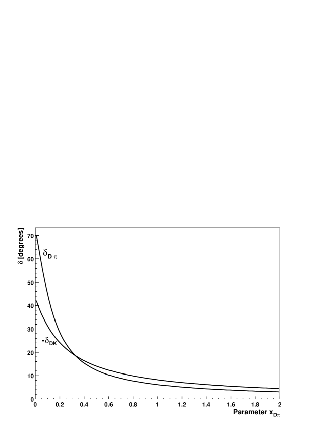
Figure 1: Final state interaction phases in $B\to D\pi$ and $B\to DK$ as a function of the Regge variable $x_{D\pi}$ defined in Eq.(7).

References

- [1] CLEO Collaboration, S. Ahmed et al, Phys. Rev. D 66, 031101(R) (2002).
- [2] Belle Collaboration, P. Krokovny, et al., Phys. Rev. Lett. 90, 1418002 (2003).
- [3] Z.-Z. Xing, Eur. Phys. J. C 28, 63 (2003).
- [4] C.-W. Chiang and J. L. Rosner, Phys. Rev. D 67, 074013 (2003).
- [5] D. Delepine, J.-M. Gerard, J. Pestieau and J. Weyers, Phys. Lett. B 429, 106 (1998).
- [6] J.-M. Gerard, J. Pestieau and J. Weyers, Phys. Lett. B 436, 363 (1998).
- [7] J.-M. Gerard and J. Weyers, Eur. Phys. J. C 7, 1 (1999).
- [8] M. Suzuki and L. Wolfenstein, Phys. Rev. D 60, 074019 (1999).
- [9] J.F. Donoghue, E. Golowich, A.A. Petrov and J.M. Soares, Phys. Rev. Lett. 77 (1996) 2178; A.N. Kamal and C.W. Luo, Phys. Rev. D 57, 4275 (1998).
- [10] J.D. Bjorken, Nucl. Phys. Proc. Suppl. 11, 325 (1989).
- [11] P. Zenczykowski, Phys. Rev. D 63, 014016 (2001).
- [12] H. Zheng, Phys. Lett. B 356, 107 (1995).
- [13] Belle Collaboration, S.K. Swain et al., Phys. Rev. D 68, 051101(R) (2003).
- [14] See however R. Fleischer, hep-ph/0310081 (oct. 2003) and references therein.
- [15] J.-M. Gerard and C. Smith, Eur. Phys. J. C 30, 69 (2003).