Fermion Masses and Coupling Unification in $E_{6}$.
Life in the Desert

Abstract

We present an $E_{6}$ Grand Unified model with a realistic pattern of fermion masses. All standard model fermions are unified in three fundamental $27$-plets (i.e. supersymmetry is not invoked), which involve in addition right handed neutrinos and three families of vector like heavy quarks and leptons. The lightest of those can lie in the low TeV range, being accessible to future collider experiments. Due to the high symmetry, the masses and mixings of all fermions are closely related. The new heavy fermions play a crucial role for the quark and lepton mass matrices and the bilarge neutrino oscillations. In all channels generation mixing and ${\cal CP}$ violation arise from a single antisymmetric matrix. The $E_{6}$ breaking proceeds via an intermediate energy region with $SU(3)_{L}\times SU(3)_{R}\times SU(3)_{C}$ gauge symmetry and a discrete left-right symmetry. This breaking pattern leads in a straightforward way to the unification of the three gauge coupling constants at high scales, providing for a long proton lifetime. The model also provides for the unification of the top, bottom and tau Yukawa couplings and for new interesting relations in flavor and generation space.

The exceptional group $E_{6}$ E6 , eric is the preferred group for Grand Unification. All Standard Model (SM) fermions are in the lowest ${\bf 27}$ representation. Its maximal subgroup $SU(3)\times SU(3)\times SU(3)$ can be viewed as an extension of the Weinberg-Salam group $SU(2)_{L}\times U(1)_{Y}\times SU(3)_{C}\to SU(3)_{L}\times SU(3)_{R}\times SU(3)_{C}\equiv G_{333}$. The fermions can be described by singlet and triplet representations of the $SU(3)$ groups only. Using for all fermion fields left handed two component Weyl spinor fields, the quantum number assignments are (for each generation) ft1 :

$${\rm Quarks}: ~{}~{}~{}Q_{L}(x)=(3,1,\bar{3})~{},$$

$${\rm Leptons}: ~{}~{}~{}L(x)=(\bar{3},3,1)~{},$$

$${\rm Antiquarks}: ~{}~{}~{}Q_{R}(x)=(1,\bar{3},3)~{}.$$ (.1)

The $78$ generators of $E_{6}$ consist of the three $SU(3)$ adjoint octet generators and the generators $F(3,3,3)$ and $\bar{F}(\bar{3},\bar{3},\bar{3})$ of coset $E_{6}/G_{333}$.

The beautiful cyclic symmetry of $E_{6}$ is apparent from (.1) and from the fact that $F$ takes a quark field into a lepton field, a lepton field into an antiquark field and an antiquark field into a quark field. An additional argument favoring $E_{6}$ is its appearance through compactification of the ten dimensional $E_{8}\times E_{8}$ heterotic superstring theory on a Calabi-Yau manifold. The compactification process can lead either to four dimensional $E_{6}$ gauge symmetry (which is anomaly free and left-right symmetric) or to some of $E_{6}$’s maximal subgroups CYE6 . Phenomenology of $E_{6}$ GUT attracted attention earlier E6 , eric , antE6 , and its active studies has been continued until recently newE6 . Phenomenology and properties of $G_{333}$ triunification models are also interesting SU3fromE6 .

According to (.1) one has besides the SM fermions: additional quark and antiquark fields with the same charges as the corresponding down quarks, two $SU(2)_{L}$ doublet leptons (containing additional ’active’ neutrinos), and two SM singlets - ’right handed’ neutrinos for each generation.

$SO(10)$ and $E_{6}$ Grand Unified Theories in old times usually predicted small neutrino mixings since in straightforward applications the large symmetry obtained from these groups connect the neutrino mixings with the small mixings observed in the quark sector. After the observation of large mixings in neutrino oscillations one had to return to the smaller $SU(5)$ group (the minimal version of it does not involve right handed neutrinos) or needed several Higgses of the same representation, or special composite operators and fine tuning procedures. In this paper we will show, however, that the consequent use of the fermion and scalar particle interactions and spectra of $E_{6}$ allows to construct a realistic GUT model.

We consider at first the Yukawa sector of $E_{6}$ with its symmetric and antisymmetric matrices in flavor and generation space. After defining the model, we can calculate from it the mass spectrum of ordinary and new fermions and their mixings in terms of a few parameters only. An interesting feature is that the mass matrices of quarks and leptons are strongly influenced by the flavor mixing of the SM particles with heavy fermions as was suggested by Bjorken, Pakvasa and Tuan bpt . Earlier suggestions for the mixing of the SM particles with new heavy fermions can be found in ros . Our work is done in the spirit of ref. bpt . As in this reference, our scenario favors a relatively light mass scale for some of the new particles [$10$-plets of $SO(10)$]. The lightest can lie in the low TeV region or even below. A major difference to bpt is the full use of the discrete left-right symmetry of $E_{6}$, valid at the intermediate symmetry $G_{333}$. It is broken solely by the Majorana property of very heavy neutral leptons (the right handed heavy neutrinos). The use of an antisymmetric Higgs representation proposed many years ago antE6 plays a decisive role. The corresponding antisymmetric matrix determines the generation mixing and the ${\cal CP}$ violation in all heavy and light channels (in the basis in which the up quark mass matrix is diagonal). The inclusion of all neutral leptons of $E_{6}$ allows to connect the mass matrix of the heavy neutrinos with the diagonal up quark mass matrix and the antisymmetric generation matrix. It leads to bimaximal mixings of the light neutrinos which then changes to a bilarge mixing pattern at the weak scale by renormalization effects. All mass ratios and mixing angles of light and heavy fermions are simply related to each other.

We then study the gauge coupling and top-bottom-tau unification in $E_{6}$. It is achieved by an unbroken $G_{333}$ subgroup as an intermediate symmetry. The discrete left-right ${\cal D}_{LR}$ symmetry, which is unbroken at these intermediate energies, plays also an important role. The breaking scale $M_{I}$ of the intermediate symmetry is not a free parameter, but uniquely fixed by the standard model couplings: $M_{I}\simeq 1.5\cdot 10^{13}$ GeV. $M_{I}$ also determines the scale of light and heavy neutrinos in agreement with experiment. The unification of the couplings occurs above $10^{16}$ GeV, in our specific model at $2\cdot 10^{17}$ GeV and thus suppresses proton decay. The renormalization of mass ratios, various Yukawa matrices and the scaling of the neutrino mass matrix are studied in detail.

Our model is non supersymmetric as the one in bpt . The hierarchy problem persists but it is hoped that its eventual solution would not change the basic features of our approach.

I Particle Assignments in $E_{6}$ and the Yukawa Sector

Let us first consider the lowest particle generation

$$(Q_{L})_{i}^{a}=\left(\begin{array}[]{c}u^{a}\\ d^{a}\\ D^{a}\end{array}\right)~{},~{}~{}L^{i}_{k}=\left(\begin{array}[]{ccc}L^{1}_{1}&E^{-}&e^{-}\\ E^{+}&L^{2}_{2}&\nu\\ e^{+}&\hat{\nu}&L^{3}_{3}\end{array}\right)~{},$$ (I.7)

$$~{}~{}(Q_{R})^{k}_{a}=\left(\hat{u}_{a},~{}\hat{d}_{a},~{}\hat{D}_{a}\right)~{}.$$ (I.8)

where $i,k,a=1,2,3$; $a$ is a color index. In this description $SU(3)_{L}$ acts vertically and $SU(3)_{R}$ horizontally. The charges are obtained from the operator

$$Q=(I_{3}+\frac{1}{2}Y)_{L}+(I_{3}+\frac{1}{2}Y)_{R}~{},$$ (I.9)

with $I_{3}$, $Y$ defined as usual. Before symmetry breaking equivalent forms of (I.8) can be obtained by applying left and right ${\cal U}$-spin rotations.

The charge conjugation operator interchanges left with right handed indices:

$${\cal C}(Q_{L})_{i}^{a}~{}{\cal C}^{-1}=(Q_{R})^{i}_{a}~{},~{}~{}~{}{\cal C}L^{i}_{k}~{}{\cal C}^{-1}=L^{k}_{i}~{},$$

$${\cal C}(Q_{R})^{i}_{a}~{}{\cal C}^{-1}=(Q_{L})_{i}^{a}~{}.$$ (I.10)

It leaves the commutation relations for the $E_{6}$ generators unchanged and is often called ${\cal D}_{LR}$ parity. The new lepton fields $L^{1}_{1}$, $L^{2}_{2}$, $L^{3}_{3}$ are identical with their own antiparticle fields. Nevertheless, if two of these fields, say $L^{1}_{1}$ and $L^{2}_{2}$, are connected by a single mass term a four component Dirac field can be formed. The two fields then behave like a (vector like) particle-antiparticle pair. The parity and ${\cal CP}$ operations change the left handed two component fields into right handed ones:

$${\cal P}(Q_{L})_{i}^{a}(t,{\rm x}){\cal P}^{-1}=\sigma_{2}(Q_{R})^{i*}_{a}(t,-{\rm x})~{},$$

$${\cal P}L^{i}_{k}(t,{\rm x}){\cal P}^{-1}=\sigma_{2}L^{k*}_{i}(t,-{\rm x})~{},$$

$${\cal P}(Q_{R})^{i}_{a}(t,{\rm x}){\cal P}^{-1}=\sigma_{2}(Q_{L})^{a*}_{i}(t,-{\rm x})~{},$$

$${\cal CP}(Q_{L})_{i}^{a}(t,{\rm x}){\cal CP}^{-1}=\sigma_{2}(Q_{L})^{a*}_{i}(t,-{\rm x})~{},$$

$${\cal CP}L^{i}_{k}(t,{\rm x}){\cal CP}^{-1}=\sigma_{2}L^{i*}_{k}(t,-{\rm x})~{},$$

$${\cal CP}(Q_{R})^{i}_{a}(t,{\rm x}){\cal CP}^{-1}=\sigma_{2}(Q_{R})^{i*}_{a}(t,-{\rm x})~{}.$$ (I.11)

By including the generation quantum number $\alpha$($=1,2,3$) all basic fermions are now classified by the left handed Weyl fields $\Psi^{\alpha}_{r}$ with the $E_{6}$ flavor index $r$ running from $1$ to $27$.

The product of two ${\bf 27}$’s of $E_{6}$ decomposes into a symmetric $\overline{\bf 27}$, an antisymmetric $\overline{\bf 351}_{A}$ and a symmetric $\overline{\bf 351}_{S}$ representation

$${\bf 27}\times{\bf 27}=\overline{\bf 27}+\overline{\bf 351}_{A}+\overline{\bf 351}_{S}~{}.$$ (I.12)

Consequently, the Yukawa interactions in the $E_{6}$ Lagrangian contein in general the three Higgs fields

$$H=H(27)~{},~{}~{}H_{A}=H(351_{A})~{},~{}~{}H_{S}=H(351_{S})~{}.$$ (I.13)

Each of the three Higgs fields couple to the fermions together with a $3\times 3$ matrix $G$ acting on the generation space

$$G_{\alpha\beta}=[G(27)]_{\alpha\beta}~{},~{}~{}~{}A_{\alpha\beta}=[G(351_{A})]_{\alpha\beta}~{},$$

$$S_{\alpha\beta}=[G(351_{S})]_{\alpha\beta}~{}.$$ (I.14)

The $E_{6}$ invariant Yukawa interaction reads

$${\cal L}_{Y}=\left((\Psi^{\alpha}_{r})^{T}{\rm i}\sigma_{2}\Psi^{\beta}_{s}\right)\left[G_{\alpha\beta}H_{rs}+A_{\alpha\beta}(H_{A})_{rs}+\right.$$

$$\left.S_{\alpha\beta}(H_{S})_{rs}\right]+{\rm h.c.}$$ (I.15)

$G$ and $S$ are symmetric matrices in generation space, while $A$ is an antisymmetric matrix. ${\cal L}_{Y}$ is invariant with respect to ${\cal C}$, the right$\leftrightarrow$left operation. In case of real vacuum expectation values (VEVs) of the Higgs fields, the part of ${\cal L}_{Y}$ obtained from the real part of these matrices is formally even under the ${\cal CP}$ and ${\cal P}$ operation, while the term arising from their imaginary parts is formally odd under ${\cal CP}$ and ${\cal P}$.

The decomposition of the Higgs fields with respect to the $G_{333}$ subgroup reads

$$H=(\bar{3},3,1)+(1,\bar{3},3)+(3,1,\bar{3})~{},$$ (I.16)

$$H_{A}=(\bar{3},3,1)+(1,\bar{3},3)+(3,1,\bar{3})+$$

$$(\bar{3},\bar{6},1)+(1,\bar{3},\bar{6})+(\bar{6},1,\bar{3})+(6,3,1)+(1,6,3)+$$

$$(3,1,6)+(3,8,\bar{3})+(\bar{3},3,8)+(8,\bar{3},3)~{},$$ (I.17)

$$H_{S}=(\bar{3},3,1)+(1,\bar{3},3)+(3,1,\bar{3})+$$

$$(6,\bar{6},1)+(1,6,\bar{6})+(\bar{6},1,6)+$$

$$(3,8,\bar{3})+(\bar{3},3,8)+(8,\bar{3},3)~{}.$$ (I.18)

The color singlet parts who’s neutral members can develop VEVs are

$$H\to(\bar{3},3,1)~{},$$

$$H_{A}\to(\bar{3},3,1)+(\bar{3},\bar{6},1)+(6,3,1)~{},$$

$$H_{S}\to(\bar{3},3,1)+(6,\bar{6},1)~{}.$$ (I.19)

We note that the parts containing a sextet or antisextet representation can only couple to leptons.

II The Model

The vacuum expectation values of the three Higgs fields determine the particle spectrum. To be in accord with the SM the masses of the new particles of $E_{6}$ have to get heavy (at least of order TeV). Thus, Higgs components which are $SU(2)_{L}$ singlets can have large VEVs. The members of $SU(2)_{L}$ doublets, on the other hand, should be of the order of the weak scale, while the VEVs of $SU(2)_{L}$ triplets are expected to vanish.

In order to define our model to be predictive and to have very few unknown parameters, we need some specific assumptions concerning the three Higgs fields, about the generation matrices $G$, $A$, $S$ and the symmetry breaking pattern. We do not consider Higgs field components which carry color. They are supposed to aquire masses of the order of the GUT scale from appropriate Higgs potentials.

We allow VEVs for all color singlet and neutral components of $H$

$$\langle H_{1}^{1}\rangle=e^{1}_{1}~{},~{}~{}~{}\langle H^{i}_{k}\rangle=e^{i}_{k}~{},~{}~{}~{}{\rm for}~{}i,k=2,3~{}.$$ (II.1)

However, by a biunitary left and right ${\cal U}$-spin transformation in flavor space (i.e. on the $SU(3)_{L}$ and $SU(3)_{R}$ indices $2$ and $3$) we can choose a proper basis for which

$$e^{2}_{3}=e^{3}_{2}=0.$$ (II.2)

Our first assumption concerns the VEVs of $H_{A}$ and $H_{S}$. $\langle H_{A}\rangle$ can mix the standard model particles with the new heavy $D$ and $L$ states [the $10$-plet of $SO(10)$]: $d\leftrightarrow D$, $e\leftrightarrow E$, $\nu=L^{2}_{3}\leftrightarrow L^{2}_{2}$. This is achieved by components of $H_{A}$ which involve left and right ${\cal U}$-spin $1/2$ indices. For the $(\bar{3},3,1)$ sector of $H_{A}$ we take, therefore,

$$\langle(H_{A})^{i}_{k}\rangle=f^{i}_{k}~{},~{}~{}~{}~{}~{}~{}~{}i,k=2,3~{}.$$ (II.3)

For the $(\bar{3},\bar{6},1)$ sector of $H_{A}$ one has correspondingly

$$\langle H_{A}^{i\{1,k\}}\rangle=f^{i\{1,k\}}~{},~{}~{}~{}~{}~{}~{}~{}i,k=2,3~{},$$ (II.4)

and for the sector $(6,3,1)$

$$\langle H_{A\{1,k\}i}\rangle=f_{\{1,k\}i}~{},~{}~{}~{}~{}~{}~{}~{}i,k=2,3~{}.$$ (II.5)

In our numerical treatment we will restrict the VEVs in (II.4), (II.5) to those with $i=3$, $k=2,3$ and $i=2$, $k=3$ which should be the dominant ones. With respect to ${\cal U}$-spin, $f^{3\{1,3\}}$ is the analogue of $f^{3}_{2}$. While $f^{3}_{2}$ mixes $d$ with $D$, $f^{3\{1,3\}}$ mixes $e^{-}$ with $E^{-}$ and $\nu$ with $L^{2}_{2}$.

The VEVs of the symmetric Higgs field $H_{S}$ can provide large Majorana masses for the heavy leptons $L^{3}_{2}$ and $L_{3}^{3}$. They arise from the $H_{S}(6,\bar{6},1)$ sector. Here we have to take the $SU(2)_{L}$ singlets and left and right handed ${\cal U}$-spin triplets

$$\langle(H_{S})_{\{3,3\}}^{\{2,2\}}\rangle=F^{\{2,2\}}~{},~{}~{}~{}~{}~{}\langle(H_{S})_{\{3,3\}}^{\{3,3\}}\rangle=F^{\{3,3\}}~{}.$$ (II.6)

All other components of $\langle H_{A}\rangle$ and $\langle H_{S}\rangle$ are taken to be zero or negligible in our calculations.

Of particular interest is the question of the breaking of the left-right symmetry of $E_{6}$. $F^{\{22\}}$ as obtained from $\langle H_{S}\rangle$ breaks this symmetry strongly. It could be the dominant manifestation of ${\cal D}_{LR}$ symmetry breaking. $\langle H\rangle$ and $\langle H_{A}\rangle$ on the other hand need not break this symmetry significantly. A strict left right symmetry in this sector would imply the relations

$$f^{i}_{k}=-f^{k}_{i}~{},~{}~{}~{}f^{i\{1,k\}}=f_{\{1,k\}i}~{},~{}~{}~{}~{}~{}i,k=2,3~{}.$$ (II.7)

The signs follow by taking the $H_{A}$ part of the Yukawa interaction to be even under ${\cal D}_{LR}$ when $H_{A}$ is replaced by $\langle H_{A}\rangle$. As a consequence of (II.7) the f’s are of the order of the weak scale even though some are standard model singlets and thus only protected by the discrete ${\cal D}_{LR}$ symmetry itself. If this is indeed the case, it implies new particles in the few TeV region as we will see.

The next assumption concerns the generation matrices $G$, $A$ and $S$. The symmetric matrix $G_{\alpha\beta}$ can be diagonalized by an orthogonal transformation, which leaves the symmetry properties of $A_{\alpha\beta}$ and $S_{\alpha\beta}$ unchanged. By choosing this basis, the up quark mass matrix is diagonal because, according to the above assumed properties of $\langle H_{A}\rangle$ and $\langle H_{S}\rangle$, only $\langle H\rangle$ contributes to it

$$\left(m_{U}\right)_{\alpha\beta}=G_{\alpha\beta}e^{1}_{1}=g_{\alpha}\delta_{\alpha\beta}e^{1}_{1}~{}.$$ (II.8)

As a consequence, the quark mixing angles and the ${\cal CP}$ violating phase must entirely come from the inclusion of the Higgs $H_{A}$ with its antisymmetric generation matrix $A_{\alpha\beta}$ as proposed in ref. antE6 . Thus, $A_{\alpha\beta}$ has to contain imaginary parts which can not be rotated away using quark phase redefinitions. This leads us to assume that the matrix $A$ is - in our phase convention - purely imaginary, i.e. a hermitian matrix. The normalized matrix contains then only two parameters, in fact only one when utilizing a discrete generation exchange symmetry for $A$ as shown later.

We suggest, that the generation matrices $G$, $A$ and $S$ are not independent of each other. In particular, the coupling matrix $S$ for the heaviest leptons should have an intimate relation with the generation matrices of the charged fermions sipar . $S$ may then be expanded in terms of $G$ and $A$. Speculatively we assume: The generation mixing matrix $S$ is a combination of the bilinear product $G^{2}$ and the commutator $[G,A]$. The generation mixing in this sector is then due to the same matrix $A$ which causes the mixing of the charged fermions. As it turns out this structure for $S$ is crucial for bilarge neutrino mixings. In fact, it leads to bimaximal mixing which is then changed to bilarge mixing by renormalization group effects.

The last assumption concerns the breaking pattern of $E_{6}$, which is presumably the origin of the breakings seen in the Yukawa sector. We suppose the following symmetry breaking chain:

$$E_{6}\stackrel{{\scriptstyle M_{\rm GUT}}}{{\longrightarrow}}SU(3)_{L}\times SU(3)_{R}\times SU(3)_{C}\times{\cal D}_{LR}\stackrel{{\scriptstyle M_{I}}}{{\longrightarrow}}$$

$$SU(2)_{L}\times U(1)_{Y}\times SU(3)_{C}~{}.$$ (II.9)

Here $M_{\rm GUT}$ is the GUT scale and ${\cal D}_{LR}$ denotes the discrete left$\leftrightarrow$right symmetry operation. As we will show below, the breaking chain (II.9) leads in a straightforward way to the unification of the gauge coupling constants. The first breaking step to the intermediate symmetry can be caused by a scalar $650$-plet which contains two $G_{333}$ singlets. One of them ${\cal S}_{+}$ is even under ${\cal D}_{LR}$ (${\cal S}_{+}\to{\cal S}_{+}$), while the second one ${\cal S}_{-}$ is odd (${\cal S}_{-}\to-{\cal S}_{-}$). It then follows from the symmetries at $M_{I}$ and above $M_{I}$ that ${\cal S}_{+}$ has the non zero VEV and $\langle{\cal S}_{-}\rangle=0$. This insures that in the $(M_{I},~{}M_{\rm GUT})$ interval $L\leftrightarrow R$ symmetry is precise and the equality of the coupling constants $g_{L}$ and $g_{R}$ is protected also at the quantum level.

We take two Higgs $SU(2)_{L}$ doublets of $H$, namely $H^{1,2}_{1}$ and $H^{1,2}_{2}$, to be relatively light. The remaining Higgs masses of the color neutral components of $H$ and $H_{A}$ are taken to be of order $M_{I}$ or higher. The only exception is the $SU(2)_{L}$ doublet $(H_{A})^{1,2}_{2}$ which can be much lighter than $M_{I}$ because of the left right symmetry ($f^{2}_{2}\approx 0$) in the $H_{A}$ sector mentioned above. But it must be heavier than $\approx 500$ TeV not to induce flavor changing processes above presently known limits. All Higgses not mentioned are assumed to have masses at the order of the GUT scale.

Before starting our investigation, let us state the quark and lepton masses at the scale $\mu=M_{Z}$ jamin , parida

$$m_{u}=(1.8\pm 0.4)~{}{\rm MeV}~{},~{}~{}~{}~{}m_{d}=(3.3\pm 0.7)~{}{\rm MeV}~{},$$

$$m_{s}=(62\pm 12)~{}{\rm MeV}~{},~{}~{}~{}~{}m_{c}=(0.64\pm 0.04)~{}{\rm GeV}~{},$$

$$m_{b}=(2.89\pm 0.03)~{}{\rm GeV}~{},~{}~{}~{}~{}m_{t}=(173\pm 5)~{}{\rm GeV}~{},$$

$$m_{e}=0.487~{}{\rm MeV}~{},~{}~{}~{}~{}m_{\mu}=102.8~{}{\rm MeV}~{},$$

$$m_{\tau}=1.747~{}{\rm GeV}~{},$$ (II.10)

as obtained from the analysis of experimental data. The general hierarchical structure of the SM masses and of the CKM matrix elements will be used in the following. Some of the masses, in particular $m_{t}$, $m_{b}$ and $m_{\tau}$, are taken as input parameters.

III The Quark Mass Matrix

Because of the hierarchical structure of the quark masses and mixing angles it is convenient to express them in terms of powers of a small dimensionless parameter. We introduce the parameter $\sigma$ sipar with the value

$$\sigma=0.058~{},$$ (III.1)

for which

$$|V_{cb}|\simeq\frac{\sigma}{\sqrt{2}}~{}~{}{\rm and}~{}~{}\left|\frac{m_{u}}{m_{c}}\right|\simeq\left|\frac{m_{c}}{m_{t}}\right|\simeq|V_{ub}|\simeq\sigma^{2}$$ (III.2)

holds within experimental uncertainties. One also has $\frac{m_{s}}{m_{b}}|V_{us}|\approx\sigma^{2}$ .

According to our assumption (II.1), (II.2) the up-quark mass matrix is

$$\left(m_{U}\right)_{\alpha\beta}\equiv G_{\alpha\beta}\langle H^{1}_{1}\rangle=g_{\alpha}\delta_{\alpha\beta}e^{1}_{1}=$$

$${\rm Diag}\left(\frac{m_{u}}{m_{t}},~{}\pm\frac{m_{c}}{m_{t}},~{}1\right)m_{t}~{}.$$ (III.3)

At the scale $\mu\simeq M_{Z}$ we can write

$$m_{U}\simeq{\rm Diag}\left(\sigma^{4},~{}\pm\sigma^{2},~{}1\right)173~{}{\rm GeV}~{}.$$ (III.4)

The signs of the mass parameters are in general of no relevance because of the freedom to change phases. But since we keep $G$ and $A$ to be hermitian matrices, the Jarlskog determinant obtained from the commutator of mass matrices depends on the sign chosen in (III.3) giving two solutions for the area of the unitarity triangle.

Because of the existence of the $D$-quarks, the down quark (big) mass matrix is a $6\times 6$ matrix, which contains the antisymmetric generation matrix $A$

$$\begin{array}[]{cc}&{\begin{array}[]{cc}\hat{d}&\hskip 42.67912pt\hat{D}\end{array}}\\ \vspace{2mm}M_{d,D}=\begin{array}[]{c}d\\ D\end{array}\!\!\!\!\!\!&{\left(\begin{array}[]{ccc}e^{2}_{2}G+f_{2}^{2}A~{},&f_{3}^{2}A\\ f_{2}^{3}A~{},&e^{3}_{3}G+f_{3}^{3}A\end{array}\right)\!}~{}.\end{array}$$ (III.5)

Here $e^{2}_{2}$, $f_{2}^{2}$ and $f_{3}^{2}$ are mass scales of order of the weak scale, while at least $e^{3}_{3}$ should describe a heavy mass scale. In accord with our model assumptions we have $f^{3}_{2},f^{3}_{3}\ll e^{3}_{3}$ which allows to integrate out the $D,\hat{D}$ states and to write down the see-saw formula

$$m_{D}\simeq e^{2}_{2}G+f_{2}^{2}A-\frac{f_{2}^{3}f_{3}^{2}}{e^{3}_{3}}\left(AG^{-1}A\right)~{}.$$ (III.6)

The $D$-quark mass matrix is simply proportional to the up quark mass matrix:

$$M_{D}\simeq e^{3}_{3}G=\frac{e^{3}_{3}}{e^{1}_{1}}m_{U}~{}.$$ (III.7)

Although eq. (III.5) should only be valid at the unification scale and has to be carefully scaled down for a determination of $m_{D}$ at $\mu\simeq M_{Z}$, we will use eq. (III.6) at $M_{Z}$ for a first orientation.

The first entry in (III.6) is responsible for the mass of the bottom quark, while the second term must provide for the small mixing angles and the large ${\cal CP}$ violating phase. The third term gives a correction to the symmetric part of the mass matrix which is important for the strange quark mass. We expect, therefore,

$$e_{2}^{2}\simeq m_{b}~{},~{}~{}~{}f_{2}^{2}|A_{23}|\simeq|V_{cb}|m_{b}~{},$$

$$f_{2}^{2}|A_{12}|\simeq m_{s}|V_{us}|~{},~{}~{}{\rm and}~{}~{}f_{2}^{2}|A_{13}|\simeq|V_{ub}|m_{b}~{}.$$ (III.8)

From (III.2) one then gets for $f^{2}_{2}$ and the generation matrix $A$

$$\begin{array}[]{cc}&{\begin{array}[]{cc}&\end{array}}\\ \vspace{2mm}f_{2}^{2}\simeq\frac{\sigma m_{b}}{\sqrt{2}\lambda_{A}}~{},~{}~{}~{}~{}~{}~{}A\simeq\begin{array}[]{c}\\ \end{array}\!\!\!\!\!\!&{\left(\begin{array}[]{ccc}0~{},&{\rm i}\sigma~{},&-{\rm i}\sigma\\ -{\rm i}\sigma~{},&0~{},&\frac{{\rm i}}{\sqrt{2}}\\ {\rm i}\sigma~{},&-\frac{{\rm i}}{\sqrt{2}}~{},&0\end{array}\right)\lambda_{A}\sqrt{2}\!}~{},\end{array}$$ (III.9)

We introduced a scaling factor $\sqrt{2}\lambda_{A}$ (as discussed in section VII) such that $f_{2}^{2}=\langle H^{2}_{2}\rangle$ and the scale dependent matrix $A$ is normalized according to ${\rm Tr}(A^{2})\simeq 2\lambda_{A}^{2}$. We remark that the antisymmetric matrix $A$ taken here is also antisymmetric with respect to the (discrete) interchange of the second generation with the third one. We know of course, that the matrix $A$ can have its strictly antisymmetric form only above $M_{I}$, the breaking point of the left-right symmetry. Thus, in our renormalization group treatment we take the matrix $A$ as given in eq. (III.9) to be strictly valid at $\mu=M_{\rm GUT}$, even though we anticipated its form at a low scale. As we will discuss in the appendix, by going down from $\mu=M_{\rm GUT}$ to $M_{I}$, the matrix $A$ ’splits’ into a matrix $A^{Q}$ for the quarks and a matrix $A^{L}$ for the leptons. By going further down to $M_{Z}$, $A^{Q}$ as well as $A^{L}$ each splits into three matrices relevant for the sectors indicated by the superscripts:

$$A^{Q}\to\left(A^{d\hat{d}}~{},~{}A^{d\hat{D}}~{},~{}A^{D\hat{d}}\right)~{}~{}~{}{\rm and}~{}~{}~{}$$

$$A^{L}\to\left(A^{e^{-}e^{+}}~{},~{}A^{e^{-}E^{+}}~{},~{}A^{E^{-}e^{+}}\right)~{}.$$ (III.10)

These matrices are no more strictly antisymmetric. Obviously, also the matrix $G$ splits into more matrices. Between $M_{\rm GUT}$ and $M_{I}$ we have $G\to\left(G_{Q},~{}G_{L}\right)$ for the quarks and leptons. Below $M_{I}$, one gets

$$G_{Q}\to\left(G^{u\hat{u}}~{},~{}G^{d\hat{d}}~{},~{}G^{D\hat{D}}\right)~{}~{}~{}{\rm and}~{}~{}~{}$$

$$G_{L}\to\left(G^{e^{+}e^{-}}~{},~{}G^{L\bar{L}}~{},~{}G^{\nu\hat{\nu}}\right)~{}.$$ (III.11)

We calculated these matrices at $\mu=M_{Z}$ in a model specified in section VII, which has a unification scale of $2\cdot 10^{17}$ GeV. The matrices $A$ are exhibited in (A.45)-(A.52). The matrix $e_{2}^{2}G$ in (III.6) becomes $e_{2}^{2}G^{d\hat{d}}$. It is obtained from $m_{U}=e_{1}^{1}G^{u\hat{u}}$ at $M_{Z}$ [eq. (III.4)] scaled up to the GUT scale, where $G^{u\hat{u}}=G^{d\hat{d}}$ holds and then scaled down to $M_{Z}$. In our approximation, it is still a diagonal matrix. In the same way, one obtains the matrix replacing $G^{-1}$ in the $D\hat{D}$ channel of eq. (III.6). It is denoted by $(G^{D\hat{D}})^{-1}$. The matrices $G^{D\hat{D}}$ and $G^{d\hat{d}}$ at $\mu=M_{Z}$ are given in (A.12), (A.33).

With these changes the mass matrix for the down quarks becomes now

$$m_{D}(M_{Z})=e_{2}^{2}G^{d\hat{d}}+f_{2}^{2}A^{d\hat{d}}-\frac{f_{2}^{3}f_{3}^{2}}{e_{3}^{3}}A^{d\hat{D}}(G^{D\hat{D}})^{-1}A^{D\hat{d}}~{}.$$

$$e_{2}^{2}(G^{d\hat{d}})_{33}\simeq m_{b}^{0}~{},~{}~{}~{}~{}~{}f_{2}^{2}(A^{d\hat{d}})_{23}\simeq\frac{{\rm i}\sigma m_{b}^{0}}{\sqrt{2}}~{}.$$ (III.12)

$m_{b}^{0}$ will slightly differ from the mass of the bottom quark because of the mixing occuring in $m_{D}$.

After having found the renormalization group effects on the matrices $G$ and $A$, the only parameter for calculating the $d$-quark masses and the CKM matrix is $f_{2}^{3}f_{3}^{2}/(e^{3}_{3}(G^{D\hat{D}})_{33})$. We use this parameter for a fit of the Cabibbo angle $|V_{us}|$. Because of our expectation of an approximate left right symmetry [see (II.7)] we look for a negative value of this parameter and find

$$\frac{f^{2}_{3}f^{3}_{2}}{e^{3}_{3}(G^{D\hat{D}})_{33}}\simeq-4.75\cdot 10^{-5}~{}{\rm GeV}~{}.$$ (III.13)

Upon diagonalization of the down quark mass matrix (III.12), with the negative sign taken in (III.4), one obtains

$$m_{d}(M_{Z})\simeq 2.66~{}{\rm MeV}~{},~{}~{}~{}~{}m_{s}(M_{Z})\simeq 49.7~{}{\rm MeV}~{},$$

$$m_{b}(M_{Z})\simeq 2.89~{}{\rm GeV}~{},$$

$$|V_{us}|\simeq 0.217~{},~{}~{}|V_{cb}|\simeq 0.045~{},~{}~{}|V_{ub}|\simeq 0.0034~{},~{}~{}~{}~{}~{}~{}~{}$$ (III.14)

and for the angles of the unitarity triangle

$$\alpha\simeq 84^{o}~{},~{}~{}~{}~{}~{}\beta\simeq 20^{o}~{},~{}~{}~{}~{}~{}\gamma\simeq 76^{o}~{}.$$ (III.15)

To obtain the correct value for $m_{b}(M_{Z})$ we took for the (3,3) element of $e_{2}^{2}G^{d\hat{d}}$, $m_{b}^{0}=2.859$ GeV. A similar good fit is obtained if in (III.4) the positive sign is chosen. The number given in (III.13) then changes to $-3.26\cdot 10^{-5}$ GeV and the angles of the unitarity triangle become

$$\alpha\simeq 95^{o}~{},~{}~{}~{}~{}~{}\beta\simeq 21^{o}~{},~{}~{}~{}~{}~{}\gamma\simeq 64^{o}~{}.$$ (III.16)

In the following we will use the negative sign in (III.4).

The results (III.14)-(III.16) are in good agreement with present experimental data. The mass of the strange quark is a bit low but still within the bounds of (II.10). We also see, that Weinberg’s suggestion wein

$$|V_{us}|\approx\sqrt{\frac{m_{d}}{m_{s}}}~{},$$ (III.17)

is valid. It follows from the smallness of the $(1,1)$ entry $e_{2}^{2}\sigma^{4}$ in (III.12) due to the small first generation up quark mass. We further note, that the term in $m_{D}$, which arises from the mixing with the heavy $D$-quarks, reduced the angle $\gamma$ from the originally obtained value $\simeq 90^{o}$ antE6 to a lower value.

Besides (III.13) there is no restriction on the value of $e^{3}_{3}$ except that $f^{3}_{2}/e^{3}_{3}$ has to be sufficiently small to justify the see-saw formula and thereby the near unitarity of the CKM mixing matrix. However, as mentioned in sect. 2, the VEVs $\langle H\rangle$ and $\langle H_{A}\rangle$ may approximately respect the left-right symmetry of $E_{6}$ and of the intermediate symmetry in contrast to the large VEV of $H_{S}$. This idea is supported by the small value found for $f^{2}_{2}$ in (III.9). It would be zero for a strict left right symmetry in this channel and is indeed small ($f^{2}_{2}\simeq 0.093$ GeV) compared to the weak interaction scale. One can then expect, that the product $-f^{2}_{3}f^{3}_{2}$ is not of order $M_{Z}M_{I}$ but not much higher than $(M_{Z})^{2}$. This gives us a rough estimate for $e^{3}_{3}$ and thus for the masses of the $D$ quarks.

$$e^{3}_{3}(G^{D\hat{D}})_{33}\approx\frac{2.1\cdot 10^{4}}{\rm GeV}M_{Z}^{2}~{}~{}{\rm or}~{}~{}\approx\frac{3.07\cdot 10^{4}}{\rm GeV}M_{Z}^{2}~{}.$$ (III.18)

From these relations, which are of course sensitive to the value taken for the weak scale input, we expect $e_{3}^{3}(G^{D\hat{D}})_{33}$ to be of order $(10^{7}-10^{8})$ GeV. Taking $e_{3}^{3}(G^{D\hat{D}})_{33}=4\cdot 10^{7}$ GeV as an example (and scaling effects into account), one obtains

$$M_{D1}\simeq 557~{}{\rm GeV}~{},~{}~{}~{}~{}M_{D2}\simeq 129~{}{\rm TeV}~{},$$

$$M_{D3}\simeq 4\cdot 10^{4}~{}{\rm TeV}~{}.$$ (III.19)

A more detailed discussion of the heavy fermions and their masses will be presented in section VI and in the appendix A1.

IV The Charged Lepton Mass Matrix

The charged lepton mass matrix has the same structure as the down quark mass matrix. By going from quarks to leptons $E_{6}$ Clebsch-Gordon coefficients have to be taken into account. Quarks and leptons couple to $H(\bar{3},3,1)$ according to the combination

$$q_{i}\hat{q}^{k}+\frac{1}{2}\varepsilon_{ii^{\prime}i^{\prime\prime}}\varepsilon^{kk^{\prime}k^{\prime\prime}}L^{i^{\prime}}_{k^{\prime}}L^{i^{\prime\prime}}_{k^{\prime\prime}}~{}.$$ (IV.1)

The $(\bar{3},3,1)$ sector of the Higgs field $H_{A}$ couples only to quarks, the sectors $(\bar{3},\bar{6},1)$ and $(6,3,1)$ only to leptons. Thus, the relevant $6\times 6$ matrix at the GUT scale is

$$\begin{array}[]{cc}&{\begin{array}[]{cc}e^{+}&\hskip 99.58464ptE^{+}\end{array}}\\ \vspace{2mm}M_{e,E}=\begin{array}[]{c}e^{-}\\ E^{-}\end{array}\!\!\!\!\!\!&{\left(\begin{array}[]{ccc}-e^{2}_{2}G-(f^{2\{1,3\}}-f_{\{1,3\}2})A~{},&f^{3\{1,3\}}A\\ -f_{\{1,3\}3}A~{},&-e^{3}_{3}G+(f^{3\{1,2\}}-f_{\{1,2\}3})A\end{array}\right)\!}~{}.\end{array}$$ (IV.2)

Using the same arguments as for the down quark mass matrix the $f$’s in the diagonal elements are small compared to the main terms. After integrating out the $E$-type states, the mass matrix for the charged leptons of the SM is generated and has at $\mu\simeq M_{Z}$ the form

$$m_{E}\simeq-e_{2}^{2}G^{e^{-}e^{+}}-(f^{2\{13\}}-f_{\{13\}2})A^{e^{-}e^{+}}$$

$$-\frac{f_{\{1,3\}3}f^{3\{1,3\}}}{e^{3}_{3}}A^{e^{-}E^{+}}(G^{L\bar{L}})^{-1}A^{E^{-}e^{+}}~{}.$$ (IV.3)

The first term is constructed like $e_{2}^{2}G^{d\hat{d}}$, but for leptons and given in the appendix A2. The contribution of VEVs in the second term should be as small as the corresponding term $f_{2}^{2}$ in the quark mass matrix. Diagonalizing (IV.3) one gets with

$$f^{2\{13\}}-f_{\{13\}2}\simeq 0.042~{}{\rm GeV}~{}~{}~{}{\rm and}$$

$$\frac{f_{\{1,3\}3}f^{3\{1,3\}}}{e^{3}_{3}(G^{L\bar{L}})_{33}}\simeq 12.6\cdot 10^{-5}~{}{\rm GeV}~{},$$ (IV.4)

the charged lepton masses

$$m_{e}=0.488~{}{\rm MeV}~{},~{}~{}~{}~{}m_{\mu}=102.8~{}{\rm MeV}~{},~{}~{}~{}~{}m_{\tau}=1.748~{}{\rm GeV}~{}.$$ (IV.5)

For obtaining the correct value of the tau lepton mass we took $m_{\tau}^{0}$ [the (3,3) element of $e_{2}^{2}G^{e^{-}e^{+}}$] to be $1.689$ GeV. The contributions from the first term in (IV.3) for the light generations are proportional to $\sigma^{4}$ and $\sigma^{2}$, respectively, and thus negligeably small. The muon mass receives its essential contribution from the third term in (IV.3). i.e. from the mixing with the heavy leptons. The contribution from the second and third terms to the electron mass are comparable. There is some ${\cal CP}$-violation due to the second term in (IV.3). The corresponding unitarity triangle, for charged leptons, has the angles: $~{}\alpha\simeq 43^{o}~{},~{}\beta\simeq 62^{o}~{},~{}\gamma\simeq 75^{o}~{}$. After diagonalization of the charged lepton matrix, this ${\cal CP}$ violation will affect the neutrino mixings. The charged lepton mixing angles turn out to be small $|V_{e\mu}|\simeq 0.034$, $|V_{e\tau}|\simeq 0.003$, $|V_{\mu\tau}|\simeq 0.068$. Therefore, the large neutrino mixings are not due to the mixings in the charged lepton sector but should come from the neutral lepton sector where large Majorana masses appear. In the next section it will be shown that this is indeed the case. Comparing now (III.13) with (IV.4) and taking into account (A.18) we get $\frac{f_{\{1,3\}3}f^{3\{1,3\}}}{-f^{2}_{3}f^{3}_{2}}\simeq(1.6)^{2}$. Considering the analogy of $f^{2}_{3}$ with $f_{\{1,3\}3}$ and $f^{3}_{2}$ with $f^{3\{1,3\}}$ this appears to be a reasonable value. In sections VI, VII we will use $|f_{\{1,3\}3}|\simeq|f^{3\{1,3\}}|$, $|f_{3}^{2}|\simeq|f_{2}^{3}|$, i.e. appropriate left-right symmetry in these channels.

V The Neutral Lepton Mass Matrix

The fundamental fermion representation of $E_{6}$ contains five neutral two-component fields. Thus, for three generations, the mass matrix for these neutral leptons is a $15\times 15$ matrix. According to the assumption stated in section II, it is given by

$$\begin{array}[]{ccccc}&{\begin{array}[]{ccccc}L^{2}_{3}&\hskip 28.45274ptL_{2}^{3}&\hskip 36.98866ptL_{3}^{3}&\hskip 31.2982ptL^{1}_{1}&\hskip 28.45274ptL^{2}_{2}\end{array}}\\ \vspace{2mm}M_{L}=\begin{array}[]{c}L^{2}_{3}\\ L^{3}_{2}\\ L^{3}_{3}\\ L_{1}^{1}\\ L^{2}_{2}\end{array}\!\!\!\!\!&{\left(\begin{array}[]{ccccc}0&-e^{1}_{1}G&0&-f^{3\{1,3\}}A&0\\ -e^{1}_{1}G&F^{\{2,2\}}S&0&-f_{\{1,3\}3}A&0\\ 0&0&F^{\{3,3\}}S&e^{2}_{2}G+h_{2}^{2}A&e^{1}_{1}G\\ -f^{3\{1,3\}}A^{T}&-f_{\{1,3\}3}A^{T}&e^{2}_{2}G+h_{2}^{2}A^{T}&0&e^{3}_{3}G+h_{3}^{3}A\\ 0&0&e^{1}_{1}G&e^{3}_{3}G+h_{3}^{3}A^{T}&0\end{array}\right)}~{},\end{array}\!\!$$ (V.1)

where

$$h_{2}^{2}=f^{2\{1,3\}}+f_{\{1,3\}2}~{},~{}~{}~{}~{}h_{3}^{3}=f^{3\{1,2\}}+f_{\{1,2\}3}~{},$$ (V.2)

and $L^{2}_{3}$ stands for the standard light neutrino fields. All ingredients in this matrix arising from the Higgs fields $H$ and $H_{A}$ are defined in the previous sections. We notice, however, that in the $L_{1}^{1}L_{2}^{2}$ block the contribution of the $f$s is additive. The new elements are the ones containing the symmetric generation matix $S$. They give rise to genuine Majorana mass terms and are of particular significance in the diagonalization process. The strength of the $H_{S}$ Higgs contribution to $M_{L}$ is governed by the constants $F^{\{2,2\}}$ and $F^{\{3,3\}}$ carrying right handed ${\cal U}$-spin quantum numbers. $F^{\{3,3\}}$ essentially fixes the Majorana mass for the heavy $L^{3}_{3}$ leptons which are expected to be of the order of the $SU(3)_{L}\times SU(3)_{R}$ breaking scale. The constant $F^{\{2,2\}}$ of similar strengths breaks the left-right symmetry and thus is responsible for the dominant breaking of this symmetry.

We can reduce the matrix $M_{L}$ to a $9\times 9$ matrix by knowing that $e_{3}^{3}$ is much larger than the other elements in the same row and column, in particular, if $f^{3\{1,3\}}$ and $f^{3\{1,2\}}$ are indeed of the order of the weak scale. This allows to integrate out the $L_{1}^{1}$, $L_{2}^{2}$ states. With the abbreviations

$$f=f^{3\{1,3\}}e_{1}^{1}/e_{3}^{3}~{},~{}~{}~{}\bar{f}=f_{\{1,3\}3}e_{1}^{1}/e_{3}^{3}~{},$$ (V.3)

one finds

$$\begin{array}[]{ccc}&{\begin{array}[]{ccc}~{}~{}L^{2}_{3}&\hskip 19.91684ptL_{2}^{3}&\hskip 17.07182ptL^{3}_{3}\end{array}}\\ \vspace{1mm}{M_{L}}^{\prime}=\begin{array}[]{c}L^{2}_{3}\\ L^{3}_{2}\\ L^{3}_{3}\end{array}\!\!\!\!\!&{\left(\begin{array}[]{ccccc}0&-e^{1}_{1}G&fA\\ -e^{1}_{1}G&F^{\{2,2\}}S&\bar{f}A\\ fA^{T}&\bar{f}A^{T}&F^{\{3,3\}}S\end{array}\right)}~{},\end{array}\!\!~{}~{}~{}~{}~{}$$ (V.4)

and

$$M_{L_{1}^{1}L_{2}^{2}}\approx e_{3}^{3}G~{}.$$ (V.5)

We neglected in (V.4) a correction to the (3-3) block, namely $-\frac{e^{1}_{1}}{e^{3}_{3}}e^{2}_{2}G$. It is small compared to the large eigenvalues of $F^{\{3,3\}}S$.

For values of $f^{3\{1,3\}}$ of the order of the weak scale and $F^{\{(2,2)\}},F^{\{(3,3)\}}$ near $M_{I}\approx 10^{13}$ GeV, we can again apply the see-saw mechanism and finally arrive at the $3\times 3$ Majorana matrix for the light neutrinos

$$m_{\nu}\simeq-\frac{(e^{1}_{1})^{2}}{F^{\{2,2\}}}GS^{-1}G-\frac{f^{2}}{F^{\{3,3\}}}A^{T}S^{-1}A~{},$$ (V.6)

and for the mass matrices of the heavy Majorana neutrinos

$$M_{L_{2}^{3}}\simeq F^{\{2,2\}}S~{},~{}~{}~{}~{}~{}M_{L_{3}^{3}}\simeq F^{\{3,3\}}S~{}.$$ (V.7)

Only the first term in (V.6) need to be considered, since the remaining one can safely be neglected. Therefore, the neutrino mass matrix (V.6) is mainly due to the decoupling of $L_{2}^{3}=\hat{\nu}$ states. It scales with the masses of these heavy lepton states.

We expect [see sect. 2] $S$ to be related to the two other generation matrices $G$ and $A$. The main term for $S$ should be $G^{2}$, which leads to a diagonal non degenerate mass matrix [see (V.6)]. We then add a term linear in $A$, the commutator $[G,A]$, with a tiny coefficient. It implies that also in this sector generation mixing is solely due to the antisymmetric matrix $A$. We take for $S$, divided by the overall coupling strength $\lambda_{S}$ to the Higgs field $H_{S}$, the real and bilinear construct

$$S/\lambda_{S}=G^{2}+{\rm i}x\sigma^{3}[G,A]~{},$$ (V.8)

whith the single parameter $x$. The $G^{2}$ term with its dominant element $\simeq 1$ for the $3^{\rm rd}$ generation serves for generation hierarchy and for the normalization of $S/\lambda_{S}$ (for which the $\sigma^{3}$ term in (V.8) can be neglected). With no renormalization effects included, the matrix $S$, as defined in (V.8) reads

$$\begin{array}[]{cc}&{\begin{array}[]{cc}&\end{array}}\\ \vspace{2mm}S/\lambda_{S}\simeq\begin{array}[]{c}\\ \end{array}\!\!\!\!\!\!&{\left(\begin{array}[]{ccc}\sigma^{8}~{},&-\sigma^{6}x~{},&-\sigma^{4}x\\ -\sigma^{6}x~{},&\sigma^{4}~{},&\frac{\sigma^{3}}{\sqrt{2}}x\\ -\sigma^{4}x~{},&\frac{\sigma^{3}}{\sqrt{2}}x~{},&1\end{array}\right)\!}~{}.\end{array}$$ (V.9)

In each element of (V.9) only the leading powers of $\sigma$ are shown.

By inverting the matrix $S$ defined in (V.8) and using (V.6), one finds for $m_{\nu}$

$$\begin{array}[]{cc}&{\begin{array}[]{cc}&\end{array}}\\ \vspace{2mm}m_{\nu}\simeq\begin{array}[]{c}\\ \end{array}\!\!\!\!\!\!&{\left(\begin{array}[]{ccc}-1~{},&(1-\frac{1}{\sqrt{2}}\sigma x)x~{},&-(1-\frac{1}{\sqrt{2}}\sigma x)x\\ (1-\frac{1}{\sqrt{2}}\sigma x)x~{},&x^{2}-1~{},&(x-\frac{1}{\sqrt{2}}\sigma)x\\ -(1-\frac{1}{\sqrt{2}}\sigma x)x~{},&(x-\frac{1}{\sqrt{2}}\sigma)x,&x^{2}-1\end{array}\right)\frac{(e_{1}^{1}\lambda_{\tau})^{2}}{(1-2x^{2}+\sqrt{2}x^{3}\sigma)\lambda_{S}F^{\{2,2\}}}\!}~{}.\end{array}$$ (V.10)

For the simplicity of representation (V.10) contains only the zeroth and first powers in $\sigma$. Taking the full expression makes numerically little difference. The interesting feature of $m_{\nu}$ is the fact that it produces for any value of $x\stackrel{{\scriptstyle>}}{{{}_{\sim}}}1.5$ automatically an almost perfect bimaximal neutrino mixing pattern (!) with a normal (not inverted) neutrino spectrum. By changing $x$, solely the ratio of mass square differences

$$R=\frac{m_{2}^{2}-m_{1}^{2}}{m_{3}^{2}-m_{2}^{2}}~{},$$ (V.11)

changes ($m_{i}$ denotes the three $\nu$ eigenstates mass ordered according to $m_{1}<m_{2}<m_{3}$). The experimentally observed ratio $R\approx 0.03$ is obtained for $x\simeq 3.5$.

However, for a proper calculation of the neutrino mass matrix at $\mu=M_{I}$ and $\mu=M_{Z}$, renormalization effects have to be taken into account. This is particularly necessary because of the large generation splitting of the heavy neutrino states $L_{2}^{3}=\hat{\nu}$ caused by the $G^{2}$ term in the matrix $S$. We have to integrate out these states in steps and to redefine $m_{\nu}$ in each step. We start by using (V.8) at the scale $M_{I}$ with $G=G_{L}$ and $A=A_{L}$ and proceed according to the rules given in appendix A4. It turns out that renormalization effects strongly influence the neutrino mass matrix and thus also the mixing pattern. The bimaximal mixing is changed to a bilarge mixing. The calculation is again performed for the gauge and Yukawa unification at $2\cdot 10^{17}$ GeV described in section VII. As in the examples given in ratz we find that the renormalization coefficients strongly reduce the mixing angle $\theta_{12}$ observed in solar neutrino experiments while the angle $\theta_{23}$ observed in atmospheric neutrino experiments is less affected. The renormalization coefficients also increase the value of the ratio $R$.

A good description of the known neutrino data is obtained by changing the value of our parameter $x=3.5$ to

$$x\simeq 2.8~{}.$$ (V.12)

With this value we obtain $R\simeq 0.055$. Larger values of $x$ reduce $R$. However, this would lead to a too strong reduction of the solar neutrino oscillation probability.

With $x\simeq 2.8$ one obtains for the mass matrix of the light neutrinos at $\mu=M_{Z}$

$$\begin{array}[]{cc}&{\begin{array}[]{cc}&\end{array}}\\ \vspace{2mm}m_{\nu}=-\begin{array}[]{c}\\ \end{array}\!\!\!\!\!\!&{\left(\begin{array}[]{ccc}-0.135~{},&0.67~{},&-0.62\\ 0.67~{},&3.75~{},&4.61\\ -0.62~{},&4.61~{},&2.81\end{array}\right)\frac{M_{0}}{10}\!}~{},\end{array}$$ (V.13)

with

$$M_{0}=\frac{(\lambda_{\tau}(M_{I})e_{1}^{1}(M_{I}))^{2}}{\lambda_{S}F^{\{2,2\}}}\simeq\frac{(102.17~{}{\rm GeV})^{2}}{M_{\hat{\nu}_{3}\hat{\nu}_{3}}}~{}.$$ (V.14)

Here $\lambda_{\tau}$ is the coupling of the third generation lepton to $H_{2}^{1,2}$ and $e_{1}^{1}$ is the VEV of the Higgs field $H_{1}^{1}$ as used before.

We obtain the mass squared difference observed in atmospheric neutrino experiments $\Delta m^{2}_{\rm atm}\simeq 2.5\cdot 10^{-3}~{}{\rm eV}^{2}$ when setting $M_{\hat{\nu}_{3}\hat{\nu}_{3}}\simeq 1.6\cdot 10^{14}$ GeV. It is very satisfying that this scale is of the same order of magnitude as expected from the value of $M_{I}$, the breaking point of the left-right symmetry ft2 . With this value of $M_{\hat{\nu}_{3}\hat{\nu}_{3}}$ the neutrino mass eigenvalues turn out to be

$$m_{1}=0.0023~{}{\rm eV}~{},~{}~{}m_{2}=0.0120~{}{\rm eV}~{},~{}~{}m_{3}=0.0516~{}{\rm eV}~{},$$

$$m_{2}^{2}-m_{1}^{2}\simeq 1.4\cdot 10^{-4}~{}({\rm eV})^{2}~{},$$

$$m_{3}^{2}-m_{2}^{2}\simeq 2.5\cdot 10^{-3}~{}({\rm eV})^{2}~{}.$$ (V.15)

To obtain the neutrino mixing matrix, one has to go to a basis in which the charged lepton mass matrix is diagonal. Diagonalizing (IV.3) and denoting by $\nu_{\alpha}$ the weak eigenstates ($\alpha=e,\mu,\tau$), we find from (V.13)

$$\nu_{\alpha}=U^{\nu}_{\alpha i}\nu_{i}~{},$$ (V.16)

$$\begin{array}[]{cc}&{\begin{array}[]{cc}&\end{array}}\\ \vspace{2mm}U^{\nu}_{\alpha i}\simeq\begin{array}[]{c}\\ \end{array}\!\!\!\!\!\!&{\left(\begin{array}[]{ccc}-0.2+0.86{\rm i}~{},&-0.46-0.08{\rm i}~{},&0.026\\ -0.29-0.015{\rm i}~{},&0.044+0.55{\rm i}~{},&0.78\\ 0.37-0.017{\rm i}~{},&-0.036-0.69{\rm i}~{},&0.62\end{array}\right)_{\alpha i}\!}~{}.\end{array}$$ (V.17)

Here we took a special phase choice for the neutrino flavor eigenstates such that the $3^{\rm rd}$ column has only real and positive elements.

Our results for the three mixing angles relevant in neutrino oscillation experiments as obtained from eq. (V.17) are

$$\sin^{2}\theta_{13}\simeq 6.8\cdot 10^{-4}~{},~{}~{}~{}\sin^{2}\theta_{12}\simeq 0.22~{},~{}~{}~{}\sin^{2}\theta_{23}\simeq 0.61~{}.$$ (V.18)

These values and the ratio $R\simeq 0.055$ of mass squared differences are quite close to the result valle of SuperKamiokande SK1 , SK2 , SNO sno and KamLAND KamL , the CHOOZ limit chooz and the observations of the disappearance of solar neutrinos HSG .

We can also get from (V.17) the neutrino unitarity triangle, defined in analogy with the quark unitarity triangle. It turns out to be:

$$\alpha_{\nu}\simeq 74^{o}~{},~{}~{}~{}~{}\beta_{\nu}\simeq 6^{o}~{},~{}~{}~{}~{}\gamma_{\nu}\simeq 100^{o}~{}.$$ (V.19)

The phases of the elements of the first row of $U^{\nu}$ are ’Majorana phases’ relevant for neutrinoless double $\beta$-decay experiments. With the convention used in (V.17) we get

$$\delta_{11}\simeq 103~{},~{}~{}~{}~{}\delta_{12}\simeq-170^{o}~{},~{}~{}~{}~{}\delta_{13}=0~{}.$$ (V.20)

For the the quantity $\langle m_{\nu}\rangle_{ee}$ which determines the decay rate we find

$$\langle m_{\nu}\rangle_{ee}=\left|m_{1}(U^{\nu}_{e1})^{2}+m_{2}(U^{\nu}_{e2})^{2}+m_{3}(U^{\nu}_{e3})^{2}\right|\simeq$$

$$9.5\cdot 10^{-4}~{}{\rm eV}~{}.$$ (V.21)

The matrix $U^{\nu}$, in particular its deviation from bimaximal mixing, depends via the renormalization parameters to some extent on the way unification is obtained. But a bilarge mixing with near maximal mixing in the $\mu-\tau$ sector will always result from the basic assumptions of our $E_{6}$ model outlined in section II.

VI The Desert is Blooming

In our model the masses of the heavy down quarks $D$ and the corresponding leptons $L$, which form a $10$-plets of $SO(10)$, have a generation splitting similar to the up quarks. The absolute values of these masses can not be given. However, if $\langle H_{A}\rangle$ still respects to some extent the left right symmetry of $E_{6}$ as discussed above, the lightest $D$ and $L$ states lie in the TeV region. In section VII, we present a numerical solution of the problem of the gauge and Yukawa coupling unification for $M_{\rm GUT}=2\cdot 10^{17}$ GeV and $e_{3}^{3}(G^{D\hat{D}})_{33}=3.98\cdot 10^{7}$ GeV. This solution also fixes the so far undetermined VEVs of $H$ and $H_{A}$. With the values quoted there [eq. (VII.36)], we can now directly diagonalize the $6\times 6$ matrices (III.5) and (IV.2) which determine the mixing of the SM particles with the $D$ and $L$ states. This mixing, although important for the mass matrices, does not seriously violate the unitarity relations for the SM particles. For example, the sum of the squares of the second row of the CKM matrix differs from one only by $1.2\cdot 10^{-4}$. In the charged lepton sector, the corresponding deviation amounts to $3.7\cdot 10^{-4}$.

We can list now the mass values of the new particles by using again $e_{3}^{3}(G^{D\hat{D}})_{33}=4\cdot 10^{7}$ GeV and setting $\lambda_{S}F^{\{2,2\}}=\lambda_{S}F^{\{3,3\}}=1.6\cdot 10^{14}$ GeV in accord with the neutrino results:

$$M_{D_{1}}\simeq 557~{}{\rm GeV}~{},~{}~{}~{}~{}M_{D_{2}}\simeq 129~{}{\rm TeV}~{},$$

$$M_{D_{3}}\simeq 4\cdot 10^{4}~{}{\rm TeV}~{},$$

$$M_{L_{1}}\simeq 355~{}{\rm GeV}~{},~{}~{}~{}~{}M_{L_{2}}\simeq 103~{}{\rm TeV}~{},$$

$$M_{L_{3}}\simeq 3.83\cdot 10^{4}~{}{\rm TeV}~{},$$

$$M(L^{3}_{2})_{1}\simeq 5.8\cdot 10^{5}~{}{\rm GeV}~{},~{}M(L^{3}_{2})_{2}\simeq 9.6\cdot 10^{8}~{}{\rm GeV}~{},$$

$$M(L^{3}_{2})_{3}\simeq 1.6\cdot 10^{14}~{}{\rm GeV}~{},$$

$$M(L^{3}_{3})_{1}\simeq 5.8\cdot 10^{5}~{}{\rm GeV}~{},~{}M(L^{3}_{3})_{2}\simeq 9.6\cdot 10^{8}~{}{\rm GeV}~{},$$

$$M(L^{3}_{3})_{3}\simeq 1.6\cdot 10^{14}~{}{\rm GeV}~{}.$$ (VI.1)

In the evaluation we took the most important renormalization effects into account (see section VII and the appendix). As we see, the desert is populated between the mass scales $M_{Z}$ and $M_{\rm GUT}$. The mass ratios for different generations of the standard model singlet neutrinos are even more drastic than the corresponding ratios for the $D$ quarks and the $SU(2)_{L}$ doublet heavy leptons.

Our specific unification model allows to calculate numerous properties of the old and new particles in particular those related to their decay properties. We will present here a few examples only.

From the $6\times 6$ mass matrix (III.5), for the quarks, one can calculate the coupling matrices in generation space for the couplings of the light and heavy mass eigenstates to the appropriate light Higgs field components

$$d^{T}\hskip 2.84544pt{\rm i}\sigma_{2}{\cal C}^{d\hat{d}}\hskip 2.84544pt\hat{d}\hskip 2.84544ptH_{2}^{2}~{},~{}~{}~{}~{}~{}d^{T}\hskip 2.84544pt{\rm i}\sigma_{2}{\cal C}^{d\hat{D}}\hskip 2.84544pt\hat{D}\hskip 2.84544ptH_{2}^{2}~{},$$

$$D^{T}\hskip 2.84544pt{\rm i}\sigma_{2}{\cal C}^{D\hat{d}}\hskip 2.84544pt\hat{d}\hskip 2.84544ptH_{2}^{2}~{}.$$ (VI.2)

We find, without using the remaining freedom of changing phases,

$$\begin{array}[]{cc}&{\begin{array}[]{cc}&\end{array}}\\ \vspace{2mm}{\cal C}^{d\hat{d}}\simeq\begin{array}[]{c}\\ \end{array}\!\!\!\!\!\!&{\left(\begin{array}[]{ccc}(-0.18+1.6\hskip 1.42262pt{\rm i})\cdot 10^{-4}~{},&(-0.25+7.3\hskip 1.42262pt{\rm i})\cdot 10^{-4}~{},&-(3.2+0.9\hskip 1.42262pt{\rm i})\cdot 10^{-5}\\ (7.4+0.28\hskip 1.42262pt{\rm i})\cdot 10^{-4}~{},&(3.3+1.3\hskip 1.42262pt{\rm i})\cdot 10^{-3}~{},&(-0.42+1.5\hskip 1.42262pt{\rm i})\cdot 10^{-4}\\ -(9.9+0.4\hskip 1.42262pt{\rm i})\cdot 10^{-3}~{},&-0.043+0.014\hskip 1.42262pt{\rm i}~{},&0.069+{\rm i}\end{array}\right)\!}~{},\end{array}$$ (VI.10)

$$\begin{array}[]{cc}&{\begin{array}[]{cc}&\end{array}}\\ \vspace{2mm}{\cal C}^{d\hat{D}}\simeq\begin{array}[]{c}\\ \end{array}\!\!\!\!\!\!&{\left(\begin{array}[]{ccc}0~{},&-4.4\cdot 10^{-7}~{},&0\\ -(0.3+3.4\hskip 1.42262pt{\rm i})\cdot 10^{-2}~{},&0~{},&4.1{\rm i}\cdot 10^{-6}\\ -0.77-8.9\hskip 1.42262pt{\rm i}~{},&0.39~{},&0\end{array}\right)\cdot 10^{-3}\!}~{},\end{array}$$ (VI.18)

$$\begin{array}[]{cc}&{\begin{array}[]{cc}&\end{array}}\\ \vspace{2mm}{\cal C}^{D\hat{d}}\simeq\begin{array}[]{c}\\ \end{array}\!\!\!\!\!\!&{\left(\begin{array}[]{ccc}0~{},&(0.33-3.8\hskip 1.42262pt{\rm i})\cdot 10^{-2}~{},&0.84-9.7\hskip 1.42262pt{\rm i}\\ -4.8\cdot 10^{-7}~{},&0~{},&0.43\\ 0~{},&-4.6\cdot 10^{-6}~{},&0\end{array}\right)\cdot 10^{-3}\!}~{}.\end{array}$$ (VI.26)

Of course, similar results can be derived for the lepton couplings to the Higgs fields.

For the weak interaction process $D\to u\hskip 2.84544ptW_{L}$ one can introduce the matrix ${\bf V}^{uD}$ as an extension of the CKM matrix

$$\overline{u}\hskip 2.84544pt\gamma^{\mu}(1-\gamma_{5}){\bf V}^{uD}\hskip 2.84544ptD\hskip 2.84544pt(W_{L})_{\mu}^{+}~{}.$$ (VI.27)

From (III.5) one gets

$$\begin{array}[]{cc}&{\begin{array}[]{cc}&\end{array}}\\ \vspace{2mm}{\bf V}^{uD}\simeq\begin{array}[]{c}\\ \end{array}\!\!\!\!\!\!&{\left(\begin{array}[]{ccc}-3.5\cdot 10^{-4}~{},&-0.04~{},&-1.1\cdot 10^{-4}\\ -0.95+11\hskip 1.42262pt{\rm i}~{},&0~{},&1.3\cdot 10^{-3}\\ 0.81-9.4\hskip 1.42262pt{\rm i}~{},&0.42~{},&0\end{array}\right)\cdot 10^{-3}\!}~{}.\end{array}$$ (VI.28)

There are also right handed current interactions of the standard model particles with the heavy $SU(2)_{R}$ vector bosons $W_{R}^{\pm}$

$$\overline{u}\hskip 2.84544pt\gamma^{\mu}(1+\gamma_{5}){\bf V}^{\hat{u}\hat{d}}\hskip 2.84544ptd\hskip 2.84544pt(W_{R})_{\mu}^{+}~{},$$ (VI.29)

where ${\bf V}^{\hat{u}\hat{d}}$ is slightly different but has the same structure as the CKM matrix.

Of particular interest for the decay properties of the mass eigenstates of $\hat{\nu}$ neutrinos are the Dirac masses connecting the flavor eigenstates of the light neutrinos (in a basis in which the charged lepton matrix is diagonal) with the heavy neutrinos. Using (IV.3), $e_{1}^{1}G_{L}(M_{I})$ from (A.8), (A.74), (A.75) and diagonalizing $S(M_{I})$ we obtain

$$\begin{array}[]{cc}&{\begin{array}[]{ccc}\hat{\nu}_{1}&\hskip 71.13188pt\hat{\nu}_{2}&\hskip 62.59596pt\hat{\nu}_{3}\end{array}}\\ \vspace{2mm}m^{\rm Dirac}\simeq\begin{array}[]{c}\nu_{1}\\ \nu_{2}\\ \nu_{3}\end{array}\!\!\!\!\!\!&{\left(\begin{array}[]{ccc}(1.7-10\hskip 1.42262pt{\rm i})\cdot 10^{-4}~{},&(-1.2-11\hskip 1.42262pt{\rm i})\cdot 10^{-3}~{},&-0.41-0.0099\hskip 1.42262pt{\rm i}\\ (-4.6+0.3\hskip 1.42262pt{\rm i})\cdot 10^{-3}~{},&0.033+0.32\hskip 1.42262pt{\rm i}~{},&3.8+7.7\hskip 1.42262pt{\rm i}\\ (3.3+3.9\hskip 1.42262pt{\rm i})\cdot 10^{-3}~{},&-0.034+0.041\hskip 1.42262pt{\rm i}~{},&-93.7+83.6\hskip 1.42262pt{\rm i}\end{array}\right){\rm GeV}\!}~{}.\end{array}$$ (VI.30)

VII Unification of Couplings

VII.1 Gauge coupling unification with intermediate
$SU(3)_{L}\times SU(3)_{R}\times SU(3)_{C}$ symmetry

As it is known, the SM does not lead to the unification of the gauge coupling constants. In our scenario, there are the additional Dirac fermions $D$ and $L$ below the GUT scale $M_{\rm GUT}$. However, these do not alter the unification picture of the standard model significantly. We still need to introduce an intermediate breaking scale $M_{I}$.

A large group like $E_{6}$ with high dimensional representations should first be broken by a step which lowers the symmetry considerably. It is natural to break $E_{6}$ to the maximal subgroup $SU(3)_{L}\times SU(3)_{R}\times SU(3)_{C}$. As we will see, this has the advantage that the corresponding intermediate scale is not an arbitrary parameter but fixed. The breaking at the GUT scale can be achieved in the scalar sector by a Higgs $H(650)$, which contains two $G_{333}$ singlets $(1,1,1)$, ${\cal S}_{+}$ and ${\cal S}_{-}$. ${\cal S}_{+}$ is even under ${\cal D}_{LR}$ and thus keeps the left-right symmetry, while ${\cal S}_{-}$ is odd. We have to take $\langle{\cal S}_{-}\rangle=0$ and $\langle{\cal S}_{+}\rangle$ to be different from zero for the breaking. It keeps $g_{L}=g_{R}$ [$g_{L}=g_{SU(3)_{L}}$, $g_{R}=g_{SU(3)_{R}}$] for $\mu\stackrel{{\scriptstyle>}}{{{}_{-}}}M_{I}$. The reason is, that at the intermediate scale $M_{I}$ the $SU(2)_{L}$ gauge coupling $g_{2}(\mu)$ and the hypercharge coupling $g_{1}(\mu)$ have to respect the $SU(3)_{L}\times SU(3)_{R}$ symmetry. Since the $U(1)_{Y}$ hypercharge is a combination of $Y_{L}$, $I_{3R}$ and $Y_{R}$, according to (I.9), the intermediate symmetry automatically requires the matching

$$g_{2}(M_{I})=g_{1}(M_{I})=g_{L}(M_{I})=g_{R}(M_{I})$$

$${\rm and}~{}~{}g_{L}(\mu)=g_{R}(\mu)~{}~{}{\rm for}~{}~{}\mu\stackrel{{\scriptstyle>}}{{{}_{-}}}M_{I}.$$ (VII.1)

The relation $g_{L}(\mu)=g_{R}(\mu)$ for $\mu\stackrel{{\scriptstyle>}}{{{}_{-}}}M_{I}$ holds even at the quantum level since it is protected by ${\cal D}_{LR}$ parity. As a consequence, $M_{I}$ is fixed by the meeting point of $g_{2}$ and $g_{1}$. From thereon the two curves continue as a single one up to $M_{\rm GUT}$ where $g_{L}=g_{R}$ unifies with $g_{C}=g_{SU(3)_{C}}$. For this to happen the states $H_{A}(6,3,1)$ and $H_{A}(\bar{3},\bar{6},1)$ will play a central role as we will see shortly.

The details are as follows: Below $M_{I}$, the field content consists of the fermionic generations of the standard model together with two light Higgs doublets and the three Dirac particles $D(D,~{}\hat{D})$, $L^{0}(L^{1}_{1},L_{2}^{2})$, $L^{-}(L^{1}_{2},L_{1}^{2})$. The two Higgs doublets are $H_{1}^{1,2}$, $H_{2}^{1,2}$ with $\langle H_{1}^{1}\rangle^{2}+\langle H_{2}^{2}\rangle^{2}=v_{0}^{2}\stackrel{{\scriptstyle<}}{{{}_{-}}}v^{2}=(174~{}{\rm GeV})^{2}$. $v_{0}$ will be smaller than $v$ in case an additional Higgs meson with standard model quantum numbers has a non zero VEV.

The corresponding $b$-factors for the evolution of the couplings are

$$\left(b_{1},b_{2},b_{3}\right)=\left(\frac{21}{5},-3,-7\right)~{},$$ (VII.2)

as obtained from the standard model fermions and two Higgs doublets. The additional $b$-factors for the $D$’s and $L$’s for each generation are

$$\left(b_{1},b_{2},b_{3}\right)^{D}=\left(\frac{4}{15},0,\frac{2}{3}\right)~{},~{}~{}\left(b_{1},b_{2},b_{3}\right)^{L}=\left(\frac{2}{5},\frac{2}{3},0\right)~{}.$$ (VII.3)

Apart from these additional states, there are more scalar doublets $H_{d}^{m}$ ($m=1,2,3,4$), which are involved in the construction of the fermion sector. One of them comes from $H(\bar{3},3,1)$ and the other three from $H_{A}(\bar{3},3,1)$. $H$ and $H_{A}$ also contain two isosinglet fields $H_{+}^{n}$ ($n=1,2$) carrying the same $U(1)_{Y}$ charge as $e^{+}$. If some of the corresponding states with masses $\mu(H_{d}^{m})$ and $\mu(H_{+}^{m})$ lie below $M_{I}$, each of them will contribute to the $b$-factors according to

$$\left(b_{1},b_{2},b_{3}\right)^{H_{d}}=\left(\frac{1}{10},\frac{1}{6},0\right)~{},~{}\left(b_{1},b_{2},b_{3}\right)^{H_{+}}=\left(\frac{1}{5},0,0\right).$$ (VII.4)

Four more Higgs components which are SM singlets could also be relatively light, but they do not contribute to the running of the gauge couplings. Thus, the solution of the renormalization group equation (at one loop level) for the gauge couplings at $M_{I}$ reads

$$\alpha_{a}^{-1}(M_{I})=\alpha_{a}^{-1}(M_{Z})-\frac{b_{a}}{2\pi}\ln\frac{M_{I}}{M_{Z}}$$

$$-\frac{b_{a}^{H_{d}}}{2\pi}\sum_{m}\ln\frac{M_{I}}{\mu(H_{d}^{m})}-\frac{b_{a}^{H_{+}}}{2\pi}\ln\frac{M_{I}^{2}}{\mu(H_{+}^{1})\mu(H_{+}^{2})}$$

$$-\frac{b_{a}^{D}}{2\pi}\ln\frac{M_{I}^{3}}{M_{D_{1}}M_{D_{2}}M_{D_{3}}}-\frac{b_{a}^{L}}{2\pi}\ln\frac{M_{I}^{3}}{M_{L_{1}}M_{L_{2}}M_{L_{3}}}~{}.$$ (VII.5)

Here $b_{a}^{D}$, $M_{D}$ and $b_{a}^{L}$, $M_{L}$ denote masses and $b$-factors of $D$ and $L$ states respectively. The matching of $g_{1}$ and $g_{2}$ at $M_{I}$ gives

$$\ln\frac{M_{I}}{M_{Z}}=\frac{5\pi}{18}\left(\alpha_{1}^{-1}(M_{Z})-\alpha_{2}^{-1}(M_{Z})\right)+\frac{1}{108}\sum_{m}\ln\frac{M_{I}}{\mu(H_{d}^{m})}$$

$$-\frac{1}{36}\ln\frac{M_{I}^{2}}{\mu(H_{+}^{1})\mu(H_{+}^{2})}-\frac{1}{27}\ln\frac{M_{L_{1}}M_{L_{2}}M_{L_{3}}}{M_{D_{1}}M_{D_{2}}M_{D_{3}}}~{}.$$ (VII.6)

At the GUT scale we should have $M_{L_{i}}=M_{D_{i}}$. According to sections III to V, $M_{L_{i}}\simeq M_{D_{i}}$ should hold approximately also at lower scales, since they are determined by $\langle H_{3}^{3}\rangle$. Thus, for the determination of $M_{I}$ we can safely neglect the last term in (VII.6). Taking the masses $\mu(H_{d}^{m})\simeq\mu(H_{+}^{n})\simeq M_{I}$, also the second term can be neglected. With $\alpha_{1}^{-1}(M_{Z})=59$ and $\alpha_{2}^{-1}(M_{Z})=29.6$ we then obtain for $M_{I}$, the breaking point of the intermediate symmetry, $M_{I}\simeq 1.3\cdot 10^{13}$ GeV. According to our model, however, one extra Higgs $SU(2)_{L}$ doublet, namely $(H_{A})^{1,2}_{2}$, should have a mass much below $M_{I}$, as was discusses in section II. The small VEV found for it, in section III, supported this view. Let us thus take its mass $\nu(H_{A2}^{1,2})=M_{A}=M_{D_{3}}\approx 4\cdot 10^{4}$ TeV, which is far above the lowest allowed value ($\sim 500$ TeV) and does not lead to flavor changing neutral currents. With this value, the second term in (VII.6) leads only to a slight increase of $M_{I}$: $M_{I}\simeq 1.5\cdot 10^{13}$ GeV. In general, the value of $M_{I}$ is rather stable with respect to modifications of our model concerning the Higgs sectors $H(\bar{3},3,1)$ and $H_{A}(\bar{3},3,1)$. It is highly interesting that the value obtained for $M_{I}$ is close (see ft2 ) to the phenomenologically obtained mass scale $(\lambda_{S}F^{\{2,2\}})$ necessary to describe the mass squared difference observed in atmospheric neutrino oscillations. Morever, the same scale also describes the breaking point of the left-right symmetry.

For the precise calculation of $\alpha_{L}(M_{I})=\alpha_{R}(M_{I})=\alpha_{1,2}(M_{I})$ from (VII.5), we need input masses for the $D$ quarks and the leptons $L$. The mass of the $3^{\rm rd}$ generation $D$ quark we take is based on the discussion about an approximate left-right symmetry in the $H$ and $H_{A}$ sectors. We use

$$M_{D_{3}}\simeq e_{3}^{3}(G^{D\hat{D}})_{33}\simeq 4\cdot 10^{4}~{}{\rm TeV}~{}.$$ (VII.7)

Before renormalization, the lepton $L_{3}$ has the same mass. The ratios for the generation splitting of these quarks and leptons are $\sigma^{4}:\sigma^{2}:1$. The corresponding input in eq. (VII.5) allows now to calculate the values $\alpha_{3}(M_{I})$ and $\alpha_{1}(M_{I})=\alpha_{2}(M_{I})$, which can then be used as initial conditions to go up to $M_{\rm GUT}$. After the study of the Yukawa coupling unification at $M_{\rm GUT}$, one can go back to the scales of the $D$ and $L$ states to find renormalized values for their masses (see the next section and the appendix). The corresponding change of eq. (VII.5) will little affect the values of $\alpha_{3}$ and $\alpha_{1}=\alpha_{2}$ at $M_{I}$, from which one can start again. The result is

$$\alpha_{3}^{-1}(M_{I})=\alpha_{C}^{-1}(M_{I})\simeq 31.43~{},$$

$$\alpha_{1}^{-1}(M_{I})=\alpha_{2}^{-1}(M_{I})=\alpha_{L,R}^{-1}(M_{I})=35.63~{}.$$ (VII.8)

The $D$ and $L$ masses, found this way, are quoted in section VI and have already been used in form of the mass matrices $M_{D}=e_{3}^{3}G^{D\hat{D}}$ and $M_{E}=e_{3}^{3}G^{L\bar{L}}$ in sections III and IV.

Above the scale of $M_{I}$ $G_{333}$ is unbroken and the quark-lepton states are unified together with the $D$ states in $Q_{L}(3,1,\bar{3})$, $Q_{R}(1,\bar{3},3)$ and the leptons $L$ in $L(\bar{3},3,1)$ multiplets. For the fermion masses we needed besides the VEVs from $H(\bar{3},3,1)$ also those from $H_{A}(\bar{3},3,1)$. We take the masses of these Higgses to be negligeable for scales above $M_{I}$ [similar to the mass of $H(\bar{3},3,1)$]. In fact, we have to do that because some members lie below $M_{I}$ and the full $(SU(3))^{2}$ symmetry must hold above $M_{I}$. The corresponding $b$-factors for $\mu\stackrel{{\scriptstyle>}}{{{}_{-}}}M_{I}$ are therefore

$$\left(b_{L},b_{R},b_{C}\right)^{M_{I}}=\left(-4,-4,-5\right)~{}.$$ (VII.9)

With these values the meeting point $g_{L}=g_{R}=g_{C}$ would be above the Planck scale because $b_{L}=b_{R}$ is not much different from $b_{C}$. We know, however, from our treatment of the charged lepton sector, that the vacuum expectation values of $H_{A}(6,3,1)$ and $H_{A}(\bar{3},\bar{6},1)$ play an important role. Since lying above the $M_{I}$ scale, the masses of these two Higgses are equal due to the left-right ${\cal D}_{LR}$ symmetry: $M(6,3,1)=M(\bar{3},\bar{6},1)\equiv M_{6}$. They contribute to the renormalization with the $b$-factors

$$\left(b_{L},b_{R},b_{C}\right)^{6}=\left(\frac{7}{2},\frac{7}{2},0\right)~{}.$$ (VII.10)

We now have for $\mu\stackrel{{\scriptstyle>}}{{{}_{-}}}M_{I}$

$$\alpha_{C}^{-1}(\mu)=\alpha_{3}^{-1}(M_{I})-\frac{b_{C}^{M_{I}}}{2\pi}\ln\frac{\mu}{M_{I}}~{},$$ (VII.11)

and

$$\alpha_{L,R}^{-1}(\mu)=\alpha_{L,R}^{-1}(M_{I})-\frac{b_{L,R}^{M_{I}}}{2\pi}\ln\frac{\mu}{M_{I}}$$

$$-\theta(\mu-M_{6})\frac{b_{L,R}^{6}}{2\pi}\ln\frac{\mu}{M_{6}}~{}.$$ (VII.12)

The Grand Unification Energy $M_{\rm GUT}$ can now be obtained by setting $\mu=M_{\rm GUT}$ and equating (VII.11) and (VII.12). $M_{\rm GUT}$ depends on $M_{6}$ and increases with increasing $M_{6}$. It is interesting, that even for low values of $M_{6}$ close to $M_{I}$ we get a large values for $M_{\rm GUT}$. For instance for $M_{6}\simeq 3M_{I}$ we have $M_{\rm GUT}\simeq 10^{16}$ GeV. Already for $M_{6}\simeq 5\cdot 10^{16}$ GeV we get $M_{\rm GUT}\simeq 3\cdot 10^{18}$ GeV. Therefore, in our model we have $M_{\rm GUT}\stackrel{{\scriptstyle>}}{{{}_{\sim}}}10^{16}$ GeV, which thus insures proton stability compatible with present experimental limits. But we still have to see which restrictions are forced on us by top-bottom-tau unification.

VII.2 Top-bottom-tau unification

In this section we study the running of the Yukawa couplings and their unification. We concentrate on the unification of the third generation couplings $\lambda_{t}$, $\lambda_{b}$, $\lambda_{\tau}$ for the top, bottom and tau fermions, respectively. In the SM, because of the small mixings in the quark sector, their evolution is little affected by the other couplings. In the considered model, the situation is different. Apart from the fermion couplings to $H(\bar{3},3,1)$ [first coupling in (I.15)] also couplings with $H_{A}$ are important. In particular, the Higgses $H_{A}^{6}(6,3,1)$, $H_{A}^{\bar{6}}(\bar{3},\bar{6},1)$ with common mass $M_{6}<M_{\rm GUT}$ are important for gauge coupling unification. Therefore, above the scale $M_{I}$, the following Yukawa couplings are relevant for renormalization:

$$Q_{L}G_{Q}Q_{R}~{}H+\frac{1}{2}LG_{L}L~{}H+Q_{L}A^{Q}Q_{R}~{}H_{A}$$

$$+\frac{1}{2}LA^{L}L~{}H_{A}^{6}+\frac{1}{2}L\bar{A}^{L}L~{}H_{A}^{\bar{6}}~{}.$$ (VII.13)

We have to distinguish the coupling matrices $G_{Q}$, $G_{L}$, $A^{Q}$, $A^{L}$, but have $A^{L}=\bar{A}^{L}$ due to the left-right ${\cal D}_{LR}$ symmetry which holds above $\mu=M_{I}$. The elements of the diagonal matrices $G_{Q}$, $G_{L}$ determine the masses $M_{D_{i}}$, $M_{L_{i}}$ respectively.

As a consequence of the first term in (VII.13) one has already at the $G_{333}$ level top-bottom unification: $\lambda_{t}(\mu)$ and $\lambda_{b}(\mu)$ must unify at $M_{I}$ and evolve then further as a single coupling $\lambda_{Q_{3}}(\mu)$. This coupling should then unify with $\lambda_{\tau}(\mu)=\lambda_{L_{3}}(\mu)$ at $\mu=M_{\rm GUT}$.

Below the scale $M_{I}$ the coupling matrices $G_{Q}$, $G_{L}$, $A^{Q}$ and $A^{L}=\bar{A}^{L}$ split into more matrices depending on the Higgs field components they are attached to. In an obvious notation we have

$$G_{Q}\to\left(G^{u\hat{u}}~{},~{}~{}G^{d\hat{d}}~{},~{}~{}G^{D\hat{D}}\right)~{},$$

$$G_{L}\to\left(G^{e^{-}e^{+}}~{},~{}~{}G^{L\bar{L}}~{},~{}~{}G^{\nu\hat{\nu}}\right)~{},$$

$$A^{Q}\to\left(A^{d\hat{d}},~{}~{}A^{d\hat{D}}~{},~{}~{}A^{D\hat{d}}\right)~{},$$

$$A^{L}\to\left(A^{e^{-}e^{+}}~{},~{}~{}A^{E^{-}e^{+}}~{},~{}~{}A^{e^{-}E^{+}}\right)~{}.$$ (VII.14)

We left out the matrices $A^{D\hat{D}}$, $A^{E^{-}E^{+}}$ and additional matrices from the neutral lepton sector. They are multiplied with VEVs which are -in our model- small compared to competing terms in the same channel. In the approximations we use for the renormalization the $G$ matrices remain diagonal and the diagonal elements of the matrices $A$ remain zero. Furthermore, the matrices connected to $\bar{A}^{L}$ are the same as the ones from $A^{L}$. But the matrices derived from $A^{L}=\bar{A}^{L}$ are no more strictly antisymmetric.

The most important elements of the matrices (VII.14) are the $(3,3)$ elements of the $G$’s and the $(2,3)$ and $(3,2)$ elements of the $A$’s: $(G^{u\hat{u}})_{33}=\lambda_{t}(\mu)$, $(G^{e^{-}e^{+}})_{33}=\lambda_{\tau}(\mu)$ etc. For the matrix elements of $A^{d\hat{d}}$ we define

$$(A^{d\hat{d}})_{23}={\rm i}\overline{\lambda}_{A}(\mu)~{},~{}~{}~{}~{}(A^{d\hat{d}})_{32}=-{\rm i}\hat{\lambda}_{A}(\mu)~{}.$$ (VII.15)

Clearly, we have $\overline{\lambda}_{A}(\mu)=\hat{\lambda}_{A}(\mu)$ for $\mu\stackrel{{\scriptstyle>}}{{{}_{-}}}M_{I}$.

There is a restriction from the mass of the vector boson $W$ for a combination of the VEVs multiplying the coupling matrices. With the notation

$$e^{1}_{1}=v_{0}\sin\beta~{},~{}~{}~{}~{}~{}e^{2}_{2}=v_{0}\cos\beta~{},$$ (VII.16)

the condition is

$$v_{0}^{2}+\left(f^{2}_{2}\right)^{2}+\left(f^{2}_{3}\right)^{2}+\left(f_{\{1,3\}3}\right)^{2}$$

$$+\left(f^{2\{13\}}-f_{\{13\}2}\right)^{2}=(174~{}{\rm GeV})^{2}~{}.$$ (VII.17)

Since $e_{1}^{1}$ and $e_{2}^{2}$ contribute to the masses of the third generation, the $v_{0}^{2}$ term should be the dominant one. At the scale $\mu=M_{Z}$ one has

$$\lambda_{t}(M_{Z})=\frac{m_{t}}{v_{0}\sin\beta}~{},~{}~{}~{}~{}\lambda_{b}(M_{Z})=\frac{m_{b}^{0}}{v_{0}\cos\beta}~{},$$

$$\lambda_{\tau}(M_{Z})=\frac{m_{\tau}^{0}}{v_{0}\cos\beta}~{}.$$ (VII.18)

Here $m_{b}^{0}$ and $m_{\tau}^{0}$ are a little smaller than $m_{b}$ and $m_{\tau}$ respectively, since they refer to the diagonal parts of the down quark and charged lepton mass matrices. In sections III and IV, we found $m_{b}^{0}/m_{b}\simeq 0.989$, $m_{\tau}^{0}/m_{\tau}\simeq 0.966$.

We can now set up the renormalization group equations for $\lambda_{t}$, $\lambda_{b}$, $\lambda_{\tau}$, $\overline{\lambda}_{A}$ and $\hat{\lambda}_{A}$. They are connected with each other and - due to the $SU(3)_{L}\times SU(3)_{R}$ symmetry at $\mu\stackrel{{\scriptstyle>}}{{{}_{-}}}M_{I}$ - no other coupling intervenes. Below $M_{I}$ we have for $\eta_{t}=\frac{\lambda_{t}^{2}}{4\pi}$, $\eta_{b}=\frac{\lambda_{b}^{2}}{4\pi}$, $\eta_{\tau}=\frac{\lambda_{\tau}^{2}}{4\pi}$, $\hat{\eta}_{A}=\frac{(\hat{\lambda}_{A})^{2}}{4\pi}$ and $\overline{\eta}_{A}=\frac{(\overline{\lambda}_{A})^{2}}{4\pi}$

$$2\pi\eta_{t}^{\prime}=\frac{9}{2}\eta_{t}^{2}+\frac{1}{2}\eta_{t}\eta_{b}-\eta_{t}\left(\frac{17}{20}\alpha_{1}+\frac{9}{4}\alpha_{2}+8\alpha_{3}\right)+\theta(\mu-M_{A})\frac{1}{2}\eta_{t}\hat{\eta}_{A}~{},$$ (VII.19)

$$2\pi\eta_{b}^{\prime}=\frac{9}{2}\eta_{b}^{2}+\frac{1}{2}\eta_{b}\eta_{t}+\eta_{b}\eta_{\tau}-\eta_{b}\left(\frac{1}{4}\alpha_{1}+\frac{9}{4}\alpha_{2}+8\alpha_{3}\right)+\theta(\mu-M_{A})\eta_{b}\left(\frac{1}{2}\hat{\eta}_{A}+\overline{\eta}_{A}\right)~{}~{},$$ (VII.20)

$$2\pi\eta_{\tau}^{\prime}=\frac{5}{2}\eta_{\tau}^{2}+3\eta_{\tau}\eta_{b}-\eta_{\tau}\left(\frac{9}{4}\alpha_{1}+\frac{9}{4}\alpha_{2}\right)~{},$$ (VII.21)

$$2\pi\hat{\eta}_{A}^{\prime}=\frac{1}{2}\hat{\eta}_{A}\left(\eta_{b}+\eta_{t}-\frac{1}{5}\alpha_{1}-3\alpha_{2}-16\alpha_{3}\right)+\theta(\mu-M_{A})\hat{\eta}_{A}\left(\frac{9}{2}\hat{\eta}_{A}+3\overline{\eta}_{A}-\frac{3}{20}\alpha_{1}-\frac{3}{4}\alpha_{2}\right)~{},$$ (VII.22)

$$2\pi\hskip 0.85358pt{\overline{\eta}_{A}}^{\prime}=\overline{\eta}_{A}\left(\eta_{b}-\frac{1}{10}\alpha_{1}-\frac{3}{2}\alpha_{2}-8\alpha_{3}\right)+\theta(\mu-M_{A})\overline{\eta}_{A}\left(\frac{9}{2}\overline{\eta}_{A}+3\hat{\eta}_{A}-\frac{3}{20}\alpha_{1}-\frac{3}{4}\alpha_{2}\right)~{}.$$ (VII.23)

At $\mu=M_{I}$ the matching

$$\eta_{t}=\eta_{b}\equiv\eta_{Q_{3}}~{},~{}~{}~{}\eta_{\tau}\equiv\eta_{L_{3}}~{},~{}~{}~{}\overline{\eta}_{A}=\hat{\eta}_{A}\equiv\eta_{A}~{},$$ (VII.24)

is required.

Above $M_{I}$ we have for $\eta_{Q_{3}}$, $\eta_{L_{3}}$, $\eta_{A}$ and $\eta_{AL}=\frac{(\lambda^{L}_{A})^{2}}{4\pi}$ the equations

$$2\pi\eta_{Q_{3}}^{\prime}=6\eta_{Q_{3}}^{2}+\eta_{Q_{3}}\eta_{L_{3}}+3\eta_{Q_{3}}\eta_{A}-\eta_{Q_{3}}8\left(\alpha_{L,R}+\alpha_{C}\right)~{},$$ (VII.25)

$$2\pi\eta_{L_{3}}^{\prime}=2\eta_{L_{3}}^{2}+3\eta_{L_{3}}\eta_{Q_{3}}-\eta_{L_{3}}\frac{56}{3}\alpha_{L,R}$$

$$+\theta(\mu-M_{6})3\eta_{L_{3}}\eta_{AL}~{},$$ (VII.26)

$$2\pi\eta_{A}^{\prime}=9\eta_{A}^{2}+\frac{3}{2}\eta_{A}\eta_{Q_{3}}-\eta_{A}8\left(\alpha_{L,R}+\alpha_{C}\right)~{},$$ (VII.27)

$$2\pi\eta_{AL}^{\prime}=\eta_{AL}\left(\frac{1}{2}\eta_{L_{3}}-16\alpha_{L,R}\right)+$$

$$\theta(\mu-M_{6})\eta_{AL}\left(4\eta_{AL}-\frac{14}{3}\alpha_{L,R}\right)~{}.$$ (VII.28)

${\rm i}\lambda_{A}^{L}$ is the $(2,3)$ element of $A^{L}=\bar{A}^{L}$ and is only needed above $M_{I}$. The matching condition at $M_{\rm GUT}$ for the final unification of the couplings reads

$$\eta_{Q_{3}}(M_{\rm GUT})=\eta_{L_{3}}(M_{\rm GUT})~{},~{}~{}\eta_{A}(M_{\rm GUT})=\eta_{AL}(M_{\rm GUT})~{}.$$ (VII.29)

The procedure of finding a solution with gauge and top-bottom-tau unification is the following: A given value of $M_{\rm GUT}\stackrel{{\scriptstyle>}}{{{}_{\sim}}}10^{16}$ GeV (otherwise no solution is possible) fixes $M_{6}$. Taking then trial values for $\eta_{Q_{3}}(M_{\rm GUT})$ and $\eta_{A}(M_{\rm GUT})$ and solving eqs. (VII.25)-(VII.28) gives their values at $M_{I}$. These values determine $\eta_{t}(M_{I})=\eta_{b}(M_{I})$, $\eta_{\tau}(M_{I})$ and $\overline{\eta}_{A}(M_{I})=\hat{\eta}_{A}(M_{I})$. The renormalization group equations (VII.19)-(VII.23) allow then to calculate $\lambda_{t}(M_{Z})$, $\lambda_{b}(M_{Z})$, $\lambda_{\tau}(M_{Z})$. Clearly, the input values $\eta_{Q_{3}}(M_{\rm GUT})$ and $\eta_{A}(M_{\rm GUT})$ have now to be changed such that $\lambda_{\tau}/\lambda_{b}$ becomes equal to $m_{\tau}^{0}/m_{b}^{0}$ and $\lambda_{t}$, $\lambda_{b}$ are in the perturbative region i.e. $\stackrel{{\scriptstyle<}}{{{}_{\sim}}}3$. If this can be achieved, one can calculate from (VII.18) $v_{0}^{2}$ and $\tan\beta$

$$v_{0}^{2}=\frac{m_{t}^{2}}{\lambda_{t}^{2}}+\frac{(m_{b}^{0})^{2}}{\lambda_{b}^{2}}~{},~{}~{}~{}\tan\beta=\frac{m_{t}}{m_{b}^{0}}\frac{\lambda_{b}}{\lambda_{t}}~{}.$$ (VII.30)

Of course, only solutions with $v_{0}<v=174$ GeV are acceptable.

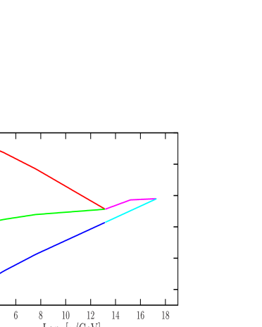
Figure 1: Unification of gauge couplings. $M_{I}\simeq 1.5\cdot 10^{13}$ GeV, $M_{6}\simeq 1.6\cdot 10^{16}$ GeV, $M_{\rm GUT}\simeq 2\cdot 10^{17}$ GeV and $\alpha_{G}^{-1}\simeq 39$.

VII.3 Numerical solution for
$M_{\rm GUT}=2\cdot 10^{17}~{}{\rm GeV}$, $M_{D_{3}}=M_{A}=4\cdot 10^{4}~{}{\rm TeV}$

Here we present a numerical solution of the problem of gauge and Yukawa coupling unification in $E_{6}$, which satisfies all above mentioned requirements. We choose the unification scale to be $2\cdot 10^{17}$ GeV, the masses of the heaviest $D$ state and the Higgs field $(H_{A})_{2}^{1,2}$ both equal to $3.98\cdot 10^{7}$ GeV.

Further imput values are the third generation masses

$$m_{t}(M_{Z})=173~{}{\rm GeV}~{},~{}~{}~{}~{}m_{b}^{0}(M_{Z})=2.859~{}{\rm GeV}~{},$$

$$m_{\tau}^{0}(M_{Z})=1.689~{}{\rm GeV}~{},$$ (VII.31)

the three gauge coupling constants at $\mu=M_{Z}$ and a suitable value for $\eta_{t,b,\tau}$ at $M_{\rm GUT}$

$$\eta_{t,b,\tau}(M_{\rm GUT})\simeq 0.0381~{}.$$ (VII.32)

For this latter value all couplings remain in the perturbative region and $v_{0}<v=174$ GeV. As a result we find the solution

$$M_{6}\simeq 1.6\cdot 10^{16}~{}{\rm GeV}~{},~{}~{}~{}~{}~{}M_{I}\simeq 1.5\cdot 10^{13}~{}{\rm GeV}~{},$$

$$\eta_{A}(M_{\rm GUT})=\eta_{AL}(M_{\rm GUT})\simeq 0.0336~{},$$ (VII.33)

with the following consequences:

$$\alpha_{G}^{-1}(M_{\rm GUT})\simeq 38.99~{},$$

$$\eta_{t,b}(M_{I})=\eta_{Q_{3}}(M_{I})\simeq 0.0412~{},$$

$$\eta_{\tau}(M_{I})=\eta_{L_{3}}(M_{I})\simeq 0.0536~{},$$

$$\hat{\eta}_{A}(M_{I})=\overline{\eta}_{A}(M_{I})=\eta_{A}(M_{I})\simeq 0.0368~{},$$

$$\eta_{AL}(M_{I})\simeq 0.0598~{},$$ (VII.34)

$$\lambda_{\tau}(M_{Z})=\lambda_{b}(M_{Z})\frac{m_{\tau}^{0}}{m_{b}^{0}}\simeq 0.612~{},~{}~{}~{}~{}~{}~{}\lambda_{t}(M_{Z})\simeq 1.127~{},$$

$$v_{0}\simeq 153.48~{}{\rm GeV}~{},~{}~{}~{}~{}~{}~{}\tan\beta\simeq 55.59~{}.$$ (VII.35)

From the value found for $v_{0}$, we can now determine $(f^{2}_{3})^{2}+(f_{\{13\}3})^{2}$ from (VII.17). Using then (III.13), (IV.4) together with $e_{3}^{3}(G^{D\hat{D}})_{33}=3.98\cdot 10^{7}$ GeV and $|f^{2}_{3}|=|f^{3}_{2}|$, $|f_{\{13\}3}|=|f^{3\{13\}}|$, we finally get

$$f_{3}^{2}=\pm 43.504~{}{\rm GeV}~{},~{}~{}~{}f_{2}^{3}=\mp 43.504~{}{\rm GeV}~{},$$

$$f_{\{13\}3}=f^{3\{13\}}=69.484~{}{\rm GeV}~{}.$$ (VII.36)

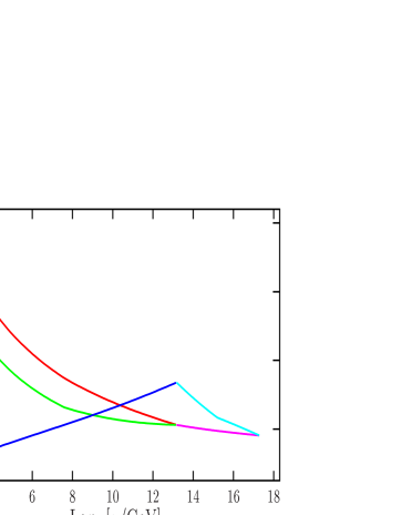
Figure 2: $t-b-\tau$ unification: $\lambda_{t}(M_{\rm GUT})=\lambda_{b}(M_{\rm GUT})=\lambda_{\tau}(M_{\rm GUT})\simeq 0.692$.

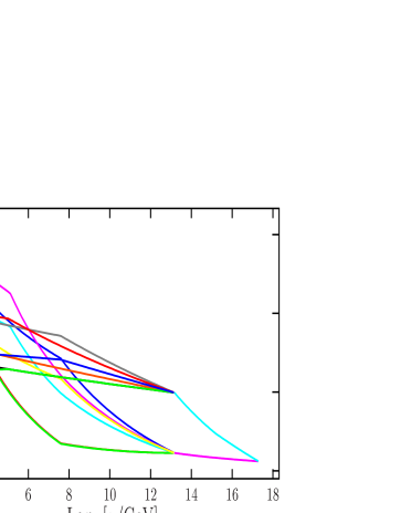
Figure 3: Unification of (2,3), (3,2) elements of $A^{Q}$ and $A^{L}$ matrices. $A^{Q}_{23}(M_{\rm GUT})=A^{L}_{23}(M_{\rm GUT})\simeq 0.65\hskip 1.42262pt{\rm i}$.

The solution for the gauge coupling and Yukawa coupling unification given here has been applied in the previous sections, in particular, for the evaluation of the renormalization parameters for all the different mass matrices.

In figure 1 -’Concorde’- we show the evolution of the gauge couplings and their unification. Figure 2 - ’Bermuda triangle’- exhibits the running of the Yukawa couplings $\eta_{t}$, $\eta_{b}$, $\eta_{\tau}$ and their unification. In figure 3 - ’desert spider’ - the running of the (2,3) and (3,2) elements of the $A$-matrices and their unification is presented. In these evaluations the splittings between the masses $M_{D_{i}}$ and $M_{L_{i}}$ (which we discuss in an appendix) have been taken into account.

VIII Conclusions

The $E_{6}$ model presented has many attractive features. Only few input data are sufficient to obtain a realistic picture of the fermion masses and their mixings. The presence of new heavy fermions in the ’desert’ plays an important role even for the mass matrices of the SM particles. All generation mixings and ${\cal CP}$ violations arise from a single antisymmetric matrix $A$, which mixes the light fermions but also the light with the heavy fermions. The latter effect also contributes in an important way to the eigenvalues of the quark and lepton mass matrices. For instance, the main part of the $\mu$ meson mass and of the strange quark mass is generated by virtual transitions to heavy fermions. As a side remark we note, that the antisymmetric generation mixing matrix found here could lead to significant effects in rare weak decay processes with fixed phases of the new contributions. The matrix $A$, in combination with $G$, is also responsible for the bilarge mixing of the light neutrinos and their oscillation pattern. In the limit of no renormalization effects, the neutrino mixing is bimaximal.

Those heavy new particles, which form $10$-plets with respect to $SO(10)$, have a hierarchical spectrum similar to the spectrum of the up quarks. The lightest ones are expected to lie in the low TeV region.

The group $E_{6}$ provides new insights about the unification of the three gauge couplings and about the unification of the Yukawa couplings of top, bottom and tau. The intermediate symmetry $SU(3)_{L}\times SU(3)_{R}\times SU(3)_{C}$ with a discrete left-right symmetry plays a decisive role. The breaking point of this intermediate symmetry is fixed by the known gauge couplings $g_{1}$ and $g_{2}$. Simultaneously it determines the mass scales for the light and heavy neutrinos. We achieved a solution of the gauge and Yukawa coupling unification with strongly constraint parameters. It describes the evolution and the final convergence of many coupling matrices which differ significantly at low energies. The solution allows to calculate quite a number of properties such as transition matrices from heavy to light fermions, Majorana phases and the double $\beta$-decay matrix element. Due to the high unification scale ($>10^{16}$ GeV), the model adequately suppresses dimension six operators which induce nucleon decays. The proton lifetime is above the presently accessible range.

The presented $E_{6}$ model can be supersymmetrized without changing the construction of the Yukawa sector. A supersymmetric version would, however, affect the coupling unification picture given here.

APPENDIX: Renormalization Analysis

A1. The $D$ and $L$ masses

In our model the $D$ and $L$ states play a crucial role for the light families. Also, the mass splitting between these states must be taken into account in the study of the gauge coupling unification. So let’s start with the renormalization of their masses. The Yukawa interactions occuring in (VII.13) obey the boundary condition $G=G_{Q}=G_{L}$ at $\mu=M_{\rm GUT}$ due to $E_{6}$ symmetry. We write

$$G_{Q}={\rm Diag}\left(\lambda_{Q_{1}}\sigma^{4}~{},~{}-\lambda_{Q_{2}}\sigma^{2}~{},~{}\lambda_{Q_{3}}\right)~{},$$ (A.1)

and

$$G_{L}={\rm Diag}\left(\lambda_{L_{1}}\sigma^{4}~{},~{}-\lambda_{L_{2}}\sigma^{2}~{},~{}\lambda_{L_{3}}\right)~{}.$$ (A.2)

For a given value for $\lambda_{Q}=\lambda_{L}$ at $M_{\rm GUT}$ the values for $\lambda_{Q_{3}}$, $\lambda_{L_{3}}$ at $\mu=M_{I}$ can be obtained using eqs. (VII.25)-(VII.28). The gauge interactions contribute to the running of $\lambda_{Q_{1(2)}}$ and $\lambda_{L_{1(2)}}$ in a similar way as for $\lambda_{Q_{3}}$ and $\lambda_{L_{3}}$. However, also the Yukawa interactions are to be taken into account. One has

$$\left.\frac{\lambda_{Q_{1}}}{\lambda_{Q_{3}}}\right|_{M_{I}}=\left.\frac{\lambda_{Q_{1}}}{\lambda_{Q_{3}}}\right|_{M_{\rm GUT}}P_{Q_{3}}^{3}P_{A}^{3}~{},$$

$$\left.\frac{\lambda_{Q_{2}}}{\lambda_{Q_{3}}}\right|_{M_{I}}=\left.\frac{\lambda_{Q_{2}}}{\lambda_{Q_{3}}}\right|_{M_{\rm GUT}}P_{Q_{3}}^{3}~{},$$ (A.3)

$$\left.\frac{\lambda_{L_{1}}}{\lambda_{L_{3}}}\right|_{M_{I}}=\left.\frac{\lambda_{L_{1}}}{\lambda_{L_{3}}}\right|_{M_{\rm GUT}}P_{L_{3}}P_{AL}^{3}~{},$$

$$\left.\frac{\lambda_{L_{2}}}{\lambda_{L_{3}}}\right|_{M_{I}}=\left.\frac{\lambda_{L_{2}}}{\lambda_{L_{3}}}\right|_{M_{\rm GUT}}P_{L_{3}}~{},$$ (A.4)

where the $P$-factors are defined as follows

$$P_{Q_{3}(L_{3},A)}=\exp\left[\frac{1}{4\pi}\int_{M_{I}}^{M_{\rm GUT}}\eta_{Q_{3}(L_{3},A)}(\mu^{\prime})d\ln\mu^{\prime}\right]~{},$$

$$P_{AL}=\exp\left[\frac{1}{4\pi}\int_{M_{6}}^{M_{\rm GUT}}\eta_{AL}(\mu^{\prime})d\ln\mu^{\prime}\right]~{}.$$ (A.5)

All numerical analysis are carried out according to the solution presented in section VII.3. The $P$-factors have the values

$$P_{Q_{3}}\simeq 1.030~{},~{}~{}~{}P_{L_{3}}\simeq 1.034~{},~{}$$

$$P_{A}\simeq 1.027~{},~{}~{}~{}~{}P_{AL}\simeq 1.015~{}.$$ (A.6)

At the scale $M_{I}$ the matrices $G_{Q}$ and $G_{L}$ are given by

$$G_{Q}(M_{I})={\rm Diag}\left(\kappa_{1}^{Q}\sigma^{4},~{}-\kappa_{2}^{Q}\sigma^{2},~{}1\right)\lambda_{Q_{3}}(M_{I})~{},$$ (A.7)

$$G_{L}(M_{I})={\rm Diag}\left(\kappa_{1}^{L}\sigma^{4},~{}-\kappa_{2}^{L}\sigma^{2},~{}1\right)\lambda_{L_{3}}(M_{I})~{},$$ (A.8)

where

$$\kappa_{1}^{Q}=\frac{1}{\kappa_{u}}P_{Q_{3}}^{3}P_{A}^{3}~{},~{}~{}~{}\kappa_{2}^{Q}=\frac{1}{\kappa_{c}}P_{Q_{3}}^{3}~{},$$

$$\kappa_{1}^{L}=\frac{1}{\kappa_{u}}P_{L_{3}}P_{AL}^{3}~{},~{}~{}~{}\kappa_{2}^{L}=\frac{1}{\kappa_{c}}P_{L_{3}}~{}.$$ (A.9)

The coefficients $\kappa_{u}$ and $\kappa_{c}$ are the factors of $\sigma^{4}$ and $\sigma^{2}$ occuring in $G$ at the GUT scale [see (A.31)] as obtained from $m_{U}$ at $\mu=M_{Z}$ [eq. (III.4)]. (A.7) and (A.8) allow to determine at $M_{I}$ the ratios $M_{D_{i}}/M_{D_{3}}$ and $M_{L_{i}}/M_{L_{3}}$ since $M_{D}\sim G_{Q}$, $M_{L}\sim G_{L}$. Below $M_{I}$ the corresponding ratios run due to gauge interactions. We have

$$\left.\frac{\lambda_{D_{1}}}{\lambda_{D_{3}}}\right|_{M_{D_{1}}}=\left.\frac{\lambda_{D_{1}}}{\lambda_{D_{3}}}\right|_{M_{I}}$$

$$\times\rho_{\alpha_{1}}^{2/5}(M_{D_{1}})\rho_{\alpha_{3}}^{8}(M_{D_{1}})\rho_{\alpha_{1}}^{-2/5}(M_{D_{3}})\rho_{\alpha_{3}}^{-8}(M_{D_{3}})~{},$$

$$\left.\frac{\lambda_{D_{2}}}{\lambda_{D_{3}}}\right|_{M_{D_{2}}}=\left.\frac{\lambda_{D_{2}}}{\lambda_{D_{3}}}\right|_{M_{I}}$$

$$\times\rho_{\alpha_{1}}^{2/5}(M_{D_{2}})\rho_{\alpha_{3}}^{8}(M_{D_{2}})\rho_{\alpha_{1}}^{-2/5}(M_{D_{3}})\rho_{\alpha_{3}}^{-8}(M_{D_{3}})~{}.$$ (A.10)

The scaling factors $\rho_{i}$ are defined in (A.25) in a similar way as the $P$-factors. In our model we find

$$\rho_{\alpha_{1}}(M_{D_{2}})\simeq 1.034~{},~{}~{}\rho_{\alpha_{3}}(M_{D_{2}})\simeq 1.066~{},$$

$$\rho_{\alpha_{1}}(M_{D_{3}})\simeq 1.025~{},~{}~{}\rho_{\alpha_{3}}(M_{D_{3}})\simeq 1.040~{}.$$ (A.11)

The ratios (A.10) do not run below the scales $\mu=M_{D_{1}}$ and $M_{D_{2}}$ respectively. Combining (A.7) and (A.10), we get for the mass ratios of the $D$-states

$$M_{D\hat{D}}=e_{3}^{3}G^{D\hat{D}}={\rm Diag}\left(\kappa^{D\hat{D}}_{1}\sigma^{4},~{}-\kappa^{D\hat{D}}_{2}\sigma^{2},~{}1\right)M_{D_{3}}~{},$$ (A.12)

$$\kappa^{D\hat{D}}_{1}\simeq 1.237~{},~{}~{}~{}~{}~{}~{}~{}~{}\kappa^{D\hat{D}}_{2}\simeq 0.965~{}.$$ (A.13)

For the mass ratios of heavy quarks to heavy leptons we have at $\mu=M_{I}$

$$\left.\frac{\lambda_{Q_{1}}}{\lambda_{L_{1}}}\right|_{M_{I}}=\left.\frac{\lambda_{Q_{3}}}{\lambda_{L_{3}}}\right|_{M_{I}}P_{Q_{3}}^{3}P_{A}^{3}P_{L_{3}}^{-1}P_{AL}^{-3}~{},$$

$$\left.\frac{\lambda_{Q_{2}}}{\lambda_{L_{2}}}\right|_{M_{I}}=\left.\frac{\lambda_{Q_{3}}}{\lambda_{L_{3}}}\right|_{M_{I}}P_{Q_{3}}^{3}P_{L_{3}}^{-1}~{}.$$ (A.14)

Using (VII.34) and (A.5), (A.14) gives

$$\left.\frac{M_{D_{1}}}{M_{L_{1}}}\right|_{M_{I}}=0.960~{},~{}~{}~{}~{}~{}~{}\left.\frac{M_{D_{2}}}{M_{L_{2}}}\right|_{M_{I}}=0.928~{}.$$ (A.15)

These values form the starting point for the further running of these mass ratios down to their own mass scale due to their gauge interactions

$$\left.\frac{M_{D_{i}}}{M_{L_{i}}}\right|_{\mu=M_{D_{i}}}=\left.\frac{M_{D_{i}}}{M_{L_{i}}}\right|_{\mu=M_{I}}\prod_{a=1}^{3}\left(\frac{\alpha_{a}(M_{I})}{\alpha_{a}(M_{D_{i}})}\right)^{\frac{\tilde{c}_{a}^{D}-\tilde{c}_{a}^{L}}{2\tilde{b}_{a}}}~{}.$$ (A.16)

$\tilde{b}_{a}$ are the $b$-factors in the interval $M_{D_{i}}-M_{I}$ and

$$\tilde{c}_{a}^{D}=\left(\frac{2}{5},0,8\right)~{},~{}~{}~{}~{}\tilde{c}_{a}^{L}=\left(\frac{9}{10},\frac{9}{2},0\right)~{},$$

$$a=(U(1)_{Y},SU(2)_{L},SU(3)_{C})~{}.$$ (A.17)

The heavy quark to heavy lepton mass ratios at their mass scales [see (VII.7), (A.12), (A.13)] are found to be

$$\frac{M_{D_{1}}}{M_{L_{1}}}=1.572~{},~{}~{}\frac{M_{D_{2}}}{M_{L_{2}}}=1.249~{},~{}~{}\frac{M_{D_{3}}}{M_{L_{3}}}=1.039~{}.$$ (A.18)

These mass splittings do only minimally affect the gauge coupling unification. Their effect is a subleading one only. By combining (A.13) and (A.18), one can find the mass ratios for the $L$-states

$$M_{L\bar{L}}=e_{3}^{3}G^{L\bar{L}}={\rm Diag}\left(\kappa^{L\bar{L}}_{1}\sigma^{4},~{}-\kappa^{L\bar{L}}_{2}\sigma^{2},~{}1\right)M_{L_{3}}~{},$$ (A.19)

with

$$\kappa^{L\bar{L}}_{1}\simeq 0.817~{},~{}~{}~{}~{}~{}~{}~{}~{}~{}\kappa^{L\bar{L}}_{2}\simeq 0.802.$$ (A.20)

Recall that in the application of our model we use $M_{D_{3}}=3.98\cdot 10^{7}$ GeV.

A2. The running of the matrices  $G^{u\hat{u}}$, $G^{d\hat{d}}$  and  $G^{e^{-}e^{+}}$

Below the scale $M_{I}$ instead of the matrix $G_{Q}$ we have two matrices: $G^{u\hat{u}}$ and $G^{d\hat{d}}$. $G^{u\hat{u}}$ accounts for the up quark Yukawa couplings. At $\mu=M_{Z}$ it is given by (III.3), (III.4). Its hierarchical structure is dictated from the values of up-type quark masses (II.10). The diagonal matrix $G^{d\hat{d}}$ describes the coupling of $q\hat{d}$ with $H_{2}^{1,2}$. The matrix $G_{L}$ is also splitted below $\mu=M_{I}$, namely to $G^{e^{-}e^{+}}$ and $G^{\nu\hat{\nu}}$, which describe the couplings $le^{+}H_{2}^{1,2}$ and $l\hat{\nu}H_{1}^{1,2}$, respectively. At the scale $M_{I}$ these couplings satisfy the conditions

$$G^{u\hat{u}}(M_{I})=G^{d\hat{d}}(M_{I})=G_{Q}(M_{I})~{},$$

$$G^{e^{-}e^{+}}(M_{I})=G^{\nu\hat{\nu}}(M_{I})=G_{L}(M_{I})~{}.$$ (A.21)

Since we have explicit information on $G^{u\hat{u}}$ at $M_{Z}$, we can calculate $G$ at the GUT scale and then derive $G^{d\hat{d}}$, $G^{e^{-}e^{+}}$ at $\mu=M_{Z}$. $G^{\nu\hat{\nu}}$ is connected with the neutrino sector, the renormalization of which is studied in appendix A4.

Below $M_{I}$ the running of the up and charm quark Yukawa couplings are due to following equations

$$4\pi\lambda_{u}^{\prime}=\lambda_{u}\left(3\eta_{t}-\frac{17}{20}\alpha_{1}-\frac{9}{4}\alpha_{2}-8\alpha_{3}\right)~{},$$ (A.22)

$$4\pi\lambda_{c}^{\prime}=\lambda_{c}\left(3\eta_{t}-\frac{17}{20}\alpha_{1}-\frac{9}{4}\alpha_{2}-8\alpha_{3}+\theta(\mu-M_{A})\frac{1}{2}\overline{\eta}_{A}\right),$$ (A.23)

It is convenient to introduce for each coupling $\eta_{i}$ ($\eta_{t},\alpha_{1},\alpha_{2},\cdots$) the quantity

$$\rho_{i}(\mu)=\exp\left[\frac{1}{4\pi}\int_{\mu}^{M_{I}}\eta_{i}(\mu^{\prime})d\ln\mu^{\prime}\right].$$ (A.24)

These scaling factors allow to express the coupling constants at arbitrary scales and thus are useful for satisfying the matching conditions on boundaries. According to (A.24), we also have

$$\exp\left[\frac{1}{4\pi}\int_{\tilde{\mu_{1}}}^{\tilde{\mu_{2}}}\eta_{i}(\mu^{\prime})d\ln\mu^{\prime}\right]=\rho_{i}(\tilde{\mu_{1}})/\rho_{i}(\tilde{\mu_{2}})~{}.$$ (A.25)

Taking all this into account, equations (VII.19), (A.22), (A.23) give

$$\left.\frac{\lambda_{u}}{\lambda_{t}}\right|_{M_{Z}}=\left.\frac{\lambda_{u}}{\lambda_{t}}\right|_{M_{I}}\rho_{t}^{3/2}(M_{Z})\rho_{b}^{1/2}(M_{Z})\rho_{\hat{\eta}_{A}}^{1/2}(M_{A})~{},$$ (A.26)

$$\left.\frac{\lambda_{c}}{\lambda_{t}}\right|_{M_{Z}}=\left.\frac{\lambda_{c}}{\lambda_{t}}\right|_{M_{I}}\rho_{t}^{3/2}(M_{Z})\rho_{b}^{1/2}(M_{Z})\rho_{\hat{\eta}_{A}}^{1/2}(M_{A})\rho_{\overline{\eta}_{A}}^{-1/2}(M_{A}).$$ (A.27)

At the scale $M_{I}$ the ratios $\lambda_{u,c}/\lambda_{t}$ can be expressed by $\left.\frac{\lambda_{Q_{1,2}}}{\lambda_{Q_{3}}}\right|_{M_{\rm GUT}}$ according to (A.3). Therefore, we have

$$\left.\frac{\lambda_{u}}{\lambda_{t}}\right|_{M_{Z}}=\left.\frac{\lambda_{u}}{\lambda_{t}}\right|_{M_{\rm GUT}}\kappa_{u}~{},~{}~{}~{}~{}\left.\frac{\lambda_{c}}{\lambda_{t}}\right|_{M_{Z}}=\left.\frac{\lambda_{c}}{\lambda_{t}}\right|_{M_{\rm GUT}}\kappa_{c}~{},$$ (A.28)

where

$$\kappa_{u}=P_{Q_{3}}^{3}P_{A}^{3}\rho_{t}^{3/2}(M_{Z})\rho_{b}^{1/2}(M_{Z})\rho_{\hat{\eta}_{A}}^{1/2}(M_{A})~{},$$

$$\kappa_{c}=\kappa_{u}P_{A}^{-3}\rho_{\overline{\eta}_{A}}^{-1/2}(M_{A})~{}.$$ (A.29)

Numerically we find in our specific model

$$\rho_{t}(M_{Z})\simeq 1.130~{},~{}~{}~{}\rho_{b}(M_{Z})\simeq 1.112~{},$$

$$\rho_{\hat{\eta}_{A}}(M_{A})\simeq\rho_{\overline{\eta}_{A}}(M_{A})\simeq 1.040~{}.$$ (A.30)

Consequently, if $G$ has at $\mu=M_{Z}$ the form given in (III.4), we have to take at the GUT scale

$$G(M_{\rm GUT})={\rm Diag}\left(\frac{1}{\kappa_{u}}\sigma^{4},~{}-\frac{1}{\kappa_{c}}\sigma^{2},~{}1\right)\cdot\lambda_{t}(M_{\rm GUT})~{}.$$ (A.31)

Our model gives

$$\kappa_{u}\simeq 1.528~{},~{}~{}~{}~{}~{}\kappa_{c}\simeq 1.386~{}.$$ (A.32)

From (A.31), it is easy to derive $G^{d\hat{d}}$ and $G^{e^{-}e^{+}}$ at the scale $M_{Z}$. The result is

$$G^{d\hat{d}}(M_{Z})={\rm Diag}\left(\kappa^{d\hat{d}}_{1}\sigma^{4},~{}-\kappa^{d\hat{d}}_{2}\sigma^{2},~{}1\right)\cdot\lambda_{b}(M_{Z})~{},$$ (A.33)

$$G^{e^{-}e^{+}}(M_{Z})={\rm Diag}\left(\kappa^{e^{-}e^{+}}_{1}\sigma^{4},~{}-\kappa^{e^{-}e^{+}}_{2}\sigma^{2},~{}1\right)\cdot\lambda_{\tau}(M_{Z})~{},$$ (A.34)

with

$$\kappa^{d\hat{d}}_{1}=\rho_{b}(M_{Z})\rho_{t}^{-1}(M_{Z})\rho_{\overline{\eta}_{A}}(M_{A})~{},$$

$$\kappa^{d\hat{d}}_{2}=\rho_{b}(M_{Z})\rho_{t}^{-1}(M_{Z})\rho_{\overline{\eta}_{A}}(M_{A})\rho^{-1}_{\hat{\eta}_{A}}(M_{A})~{},$$ (A.35)

$$\kappa^{e^{-}e^{+}}_{1}=\frac{1}{\kappa_{u}}P_{L_{3}}P_{AL}^{3}\rho^{3/2}_{\tau}(M_{Z})~{},$$

$$\kappa^{e^{-}e^{+}}_{2}=\frac{1}{\kappa_{c}}P_{L_{3}}\rho^{3/2}_{\tau}(M_{Z})~{}.$$ (A.36)

The numerical values of these factors are

$$\kappa^{d\hat{d}}_{1}=1.023~{},~{}~{}~{}\kappa^{d\hat{d}}_{2}=0.984~{},$$

$$\kappa^{e^{-}e^{+}}_{1}=0.804~{},~{}~{}~{}\kappa^{e^{-}e^{+}}_{2}=0.848~{}.$$ (A.37)

A3. Renormalization of $A^{Q}$, $A^{L}$ matrix elements

At the scale $M_{\rm GUT}$ the antisymmetric matrix $A$, which describes the fermion couplings with the components of the Higgs field $H_{A}$, is postulated to have the form

$$\begin{array}[]{cc}&{\begin{array}[]{cc}&\end{array}}\\ \vspace{2mm}A(M_{\rm GUT})=\begin{array}[]{c}\\ \end{array}\!\!\!\!\!\!&{\left(\begin{array}[]{ccc}0~{},&{\rm i}\sigma~{},&-{\rm i}\sigma\\ -{\rm i}\sigma~{},&0~{},&\frac{{\rm i}}{\sqrt{2}}\\ {\rm i}\sigma~{},&-\frac{{\rm i}}{\sqrt{2}}~{},&0\end{array}\right)\lambda_{A}\sqrt{2}\!}~{}.\end{array}$$ (A.38)

Between the scales $M_{I}$ and $M_{\rm GUT}$, instead of one matrix $A$ we are dealing with the two matrices $A^{Q}$ and $A^{L}=\bar{A}^{L}$ in the Yukawa interaction of (VII.13). Due to RG effects, they will differ from the original matrix $A(M_{\rm GUT})$. $A^{Q}$ and $A^{L}$ remain antisymmetric above $M_{I}$ and have the forms:

$$\begin{array}[]{cc}&{\begin{array}[]{cc}&\end{array}}\\ \vspace{2mm}A^{Q}={\rm i}\begin{array}[]{c}\\ \end{array}\!\!\!\!\!\!&{\left(\begin{array}[]{ccc}0~{},&\kappa^{Q}_{a}\sigma~{},&-\kappa^{Q}_{b}\sigma\\ -\kappa^{Q}_{a}\sigma~{},&0~{},&\frac{1}{\sqrt{2}}\\ \kappa^{Q}_{b}\sigma~{},&-\frac{1}{\sqrt{2}}~{},&0\end{array}\right)\lambda_{A}\sqrt{2}\!}~{},{}{}{}\end{array}\begin{array}[]{cc}&{\begin{array}[]{cc}&\end{array}}\\ \vspace{2mm}A^{L}={\rm i}\begin{array}[]{c}\\ \end{array}\!\!\!\!\!\!&{\left(\begin{array}[]{ccc}0~{},&\kappa^{L}_{a}\sigma~{},&-\kappa^{L}_{b}\sigma\\ -\kappa^{L}_{a}\sigma~{},&0~{},&\frac{1}{\sqrt{2}}\\ \kappa^{L}_{b}\sigma~{},&-\frac{1}{\sqrt{2}}~{},&0\end{array}\right)\lambda_{A}^{L}\sqrt{2}\!}~{}.\end{array}$$ (A.39)

Here $\kappa^{Q,L}$ and $\lambda_{A},\lambda_{A}^{L}$ are scale dependent renormalization factors, which can be determined through the RG equations of the $A^{Q}$ and $A^{L}$ matrices:

$$16\pi^{2}(A^{Q})^{\prime}=3A^{Q}A^{Q\dagger}A^{Q}+\frac{3}{2}\lambda_{Q}\lambda_{Q}^{\dagger}A^{Q}+\frac{3}{2}A^{Q}\lambda_{Q}\lambda_{Q}^{\dagger}$$

$$+A^{Q}\left(3{\rm Tr}(A^{Q}A^{Q\dagger})-8g_{L,R}^{2}-8g_{C}^{2}\right)~{},$$ (A.40)

$$16\pi^{2}(A^{L})^{\prime}=\frac{1}{2}\lambda_{L}\lambda_{L}^{\dagger}A^{L}+\frac{1}{2}A^{L}\lambda_{L}\lambda_{L}^{\dagger}-A^{L}16g_{L,R}^{2}+$$

$$\theta(\mu-M_{6})A^{L}\left(3A^{L\dagger}A^{L}+\frac{1}{2}{\rm Tr}(A^{L}A^{L\dagger})-\frac{14}{3}g_{L,R}^{2}\right)~{}.$$ (A.41)

At the scale $M_{\rm GUT}$, the boundary conditions are

$$A^{Q}(M_{\rm GUT})=A^{L}(M_{\rm GUT})~{},~{}~{}~{}~{}{\rm and}~{}~{}~{}~{}\kappa^{Q}_{a,b}=\kappa^{L}_{a,b}=1~{}.$$ (A.42)

From (A.40) and (A.41) follow the RG equations (VII.27) and (VII.28) for $\lambda_{A}$ and $\lambda_{A}^{L}$, which we solved numerically. It is easy to observe, that the ratios $A^{Q}_{13}/A^{Q}_{23}$ and $A^{L}_{13}/A^{Q}_{23}$ do not run, while the other ratios are scale dependent. For the factors $\kappa^{Q,L}$ we have at $\mu=M_{I}$

$$\kappa^{Q}_{a}=P_{Q_{3}}^{3/2}~{},~{}~{}~{}\kappa^{L}_{a}=P_{L_{3}}^{1/2}~{},~{}~{}~{}\kappa^{Q}_{b}=\kappa^{L}_{b}=1~{},$$ (A.43)

where $P_{Q_{3}}$, $P_{L_{3}}$ are given in (A.5), (A.6).

Below the scale $M_{I}$, instead of one $A^{Q}$ matrix there are matrices which represent the couplings of colored fermions with Higgs doublets and singlet. Namely:

$$Q_{L}A^{Q}Q_{R}~{}H_{A}\to A^{d\hat{d}}q\hat{d}~{}(H_{A})_{2}^{1,2}+A^{D\hat{d}}D\hat{d}~{}(H_{A})^{3}_{2}$$

$$+A^{d\hat{D}}q\hat{D}~{}(H_{A})_{3}^{1,2}~{}.$$ (A.44)

At the scale $M_{I}$ all matrices unify $A^{d\hat{d}}(M_{I})=A^{D\hat{d}}(M_{I})=A^{d\hat{D}}(M_{I})=A^{Q}(M_{I})$. There they are precisely antisymmetric and their matrix elements match with the appropriate $\kappa^{Q}_{a,b}$ factors of (A.39). RG study allow to calculate these matrices at the scale needed. Our numerical analysis gives the following results for the $A^{Q}$-matrices at the scale $\mu=M_{Z}$ (where contact with experimental data can be performed):

$$\begin{array}[]{cc}&{\begin{array}[]{cc}&\end{array}}\\ \vspace{2mm}A^{d\hat{d}}(M_{Z})\simeq{\rm i}\begin{array}[]{c}\\ \end{array}\!\!\!\!\!\!&{\left(\begin{array}[]{ccc}0~{},&1.16\sigma~{},&-\sigma\\ -1.16\sigma~{},&0~{},&\frac{1}{\sqrt{2}}\\ 0.99\sigma~{},&-\frac{0.99}{\sqrt{2}}~{},&0\end{array}\right)\overline{\lambda}_{A}(M_{Z})\sqrt{2}\!}~{},\end{array}$$ (A.45)

$$\begin{array}[]{cc}&{\begin{array}[]{cc}&\end{array}}\\ \vspace{2mm}A^{D\hat{d}}(M_{Z})\simeq{\rm i}\begin{array}[]{c}\\ \end{array}\!\!\!\!\!\!&{\left(\begin{array}[]{ccc}0~{},&1.39\sigma~{},&-1.2\sigma\\ -1.16\sigma~{},&0~{},&\frac{1}{\sqrt{2}}\\ 0.97\sigma~{},&-\frac{0.97}{\sqrt{2}}~{},&0\end{array}\right)\lambda_{A}(M_{Z})\sqrt{2}\!}~{},\end{array}$$ (A.46)

$$\begin{array}[]{cc}&{\begin{array}[]{cc}&\end{array}}\\ \vspace{2mm}A^{d\hat{D}}(M_{Z})\simeq{\rm i}\begin{array}[]{c}\\ \end{array}\!\!\!\!\!\!&{\left(\begin{array}[]{ccc}0~{},&1.19\sigma~{},&-\sigma\\ -1.42\sigma~{},&0~{},&\frac{1}{\sqrt{2}}\\ 1.21\sigma~{},&-\frac{1.02}{\sqrt{2}}~{},&0\end{array}\right)\lambda_{A}^{0}(M_{Z})\sqrt{2}\!}~{}.\end{array}$$ (A.47)

The couplings are

$$\overline{\lambda}_{A}(M_{Z})=1.262~{},~{}~{}~{}~{}\lambda_{A}(M_{Z})=1.131~{},$$

$$\lambda_{A}^{0}(M_{Z})=1.220~{}.$$ (A.48)

A similar analysis can be performed to obtain the generation mixing matrices $A^{L}$ for leptons. Below $M_{I}$ we are dealing with three types of matrices $A^{e^{-}e^{+}}$, $A^{E^{-}e^{+}}$ and $A^{e^{-}E^{+}}$. These coupling matrices are relevant for the charged lepton sector. At the scale $\mu=M_{Z}$ we find

$$\begin{array}[]{cc}&{\begin{array}[]{cc}&\end{array}}\\ \vspace{2mm}A^{e^{-}e^{+}}(M_{Z})\simeq{\rm i}\begin{array}[]{c}\\ \end{array}\!\!\!\!\!\!&{\left(\begin{array}[]{ccc}0~{},&1.11\sigma~{},&-\sigma\\ -1.11\sigma~{},&0~{},&\frac{1}{\sqrt{2}}\\ 1.04\sigma~{},&-\frac{1.04}{\sqrt{2}}~{},&0\end{array}\right)\overline{\lambda}_{A}^{L}(M_{Z})\sqrt{2}\!}~{},\end{array}$$ (A.49)

$$\begin{array}[]{cc}&{\begin{array}[]{cc}&\end{array}}\\ \vspace{2mm}A^{E^{-}e^{+}}(M_{Z})\simeq{\rm i}\begin{array}[]{c}\\ \end{array}\!\!\!\!\!\!&{\left(\begin{array}[]{ccc}0~{},&1.14\sigma~{},&-1.03\sigma\\ -1.11\sigma~{},&0~{},&\frac{1}{\sqrt{2}}\\ 1.06\sigma~{},&-\frac{1.06}{\sqrt{2}}~{},&0\end{array}\right)\lambda_{A}^{L}(M_{Z})\sqrt{2}\!}~{},\end{array}$$ (A.50)

$$\begin{array}[]{cc}&{\begin{array}[]{cc}&\end{array}}\\ \vspace{2mm}A^{e^{-}E^{+}}(M_{Z})\simeq{\rm i}\begin{array}[]{c}\\ \end{array}\!\!\!\!\!\!&{\left(\begin{array}[]{ccc}0~{},&1.07\sigma~{},&-1.05\sigma\\ -1.12\sigma~{},&0~{},&\frac{1}{\sqrt{2}}\\ 1.06\sigma~{},&-\frac{1.01}{\sqrt{2}}~{},&0\end{array}\right)\lambda_{A}^{0L}(M_{Z})\sqrt{2}\!}~{}.\end{array}$$ (A.51)

The coupling factors are

$$\overline{\lambda}_{A}^{L}(M_{Z})=0.957~{},~{}~{}~{}~{}\lambda_{A}^{L}(M_{Z})=0.923~{},$$

$$\lambda_{A}^{0L}(M_{Z})=1.068~{}.$$ (A.52)

The picture which shows the running of all $(2,3)$ and $(3,2)$ elements of the matrices $A^{Q}$ and $A^{L}$ and their final unification is presented in figure 3, the ’desert spider’.

A4. Neutrino mass matrix renormalization

Here we will perform the renormalization analysis for the neutrino sector.

Dimension five operators, responsible for neutrino masses, are generated by integrating out the ’right handed’ states $(L^{3}_{2})_{\alpha}=\hat{\nu}_{\alpha}$. The $\hat{\nu}_{\alpha}$ masses are determined by the matrix $F^{\{2,2\}}S$. The matrix $S$ describes the generation dependent Majorana couplings of these states to the symmetric sextet component of the Higgs field $H_{S}$. In our model $S$ is postulated to be the bilinear matrix product in generation space (V.8). We take this form to be valid at $M_{I}$ with $G\to G_{L}$ and $A\to A^{L}$. With the appropriate scaling factors, at $\mu=M_{I}$ the matrix $S$ has the form:

$$\begin{array}[]{cc}&{\begin{array}[]{cc}&\end{array}}\\ \vspace{2mm}S/\lambda_{S}\simeq\begin{array}[]{c}\\ \end{array}\!\!\!\!\!\!&{\left(\begin{array}[]{ccc}(\kappa^{L}_{1})^{2}\sigma^{8}~{},&-\kappa^{L}_{2}\kappa^{L}_{a}\sigma^{6}x~{},&-\sigma^{4}x\\ -\kappa^{L}_{2}\kappa^{L}_{a}\sigma^{6}x~{},&(\kappa^{L}_{2})^{2}\sigma^{4}~{},&\frac{\sigma^{3}}{\sqrt{2}}x\\ -\sigma^{4}x~{},&\frac{\sigma^{3}}{\sqrt{2}}x~{},&1\end{array}\right)\!}~{}.\end{array}$$ (A.53)

Again, as in (V.9), only the leading terms in $\sigma$ are exhibited here. The renormalization coefficients $\kappa$ are shown in (A.75). At the scale $M_{I}$, the mass matrix for the states $\hat{\nu}_{\alpha}$ is

$$M_{\hat{\nu}\hat{\nu}}^{\alpha\beta}(M_{I})=F^{\{2,2\}}S^{\alpha\beta}~{}.$$ (A.54)

The eigenvalues are $\mu_{1}\simeq\sigma^{8}\left((\kappa^{L}_{1})^{2}-(\kappa^{L}_{a})^{2}x^{2}-x^{2}+\frac{\kappa_{a}^{L}}{\kappa^{L}_{2}}\sqrt{2}x^{3}\sigma\right)\lambda_{S}F^{\{2,2\}}$, $\mu_{2}\simeq\sigma^{4}(\kappa^{L}_{2})^{2}\lambda_{S}F^{\{2,2\}}$ and $\lambda_{S}F^{\{2,2\}}$. As we can see, these scales are separated by large distances. Because of this fact strong renormalization effects occur. They are the cause of the difference between the neutrino mass matrices (V.10) and (V.13). The decoupling of the three $\hat{\nu}_{\alpha}$ states occurs step by step. Thus the renormalization has to be performed separately in each energy interval lindner , ratz . By generalizing the results of ref. ratz we present model independent formula for the running of the neutrino mass matrix $m_{\nu}$ and then apply them to our model.

The couplings in the neutrino sector involve Dirac and Majorana mass terms. One can choose a basis in which the mass matrix for the heavy neutrinos is diagonal. Thus, without loss of generality, one can write the coupling terms in the form

$$\nu_{\alpha}(\lambda^{\rm Dirac})^{\alpha\beta}\hat{\nu}_{\beta}+\frac{1}{2}\mu_{\alpha}\hat{\nu}_{\alpha}\hat{\nu}_{\alpha}~{}.$$ (A.55)

The matrix $\lambda^{\rm Dirac}$ is related to the original Dirac matrix $\lambda_{0}^{\rm Dirac}=G^{\nu\hat{\nu}}e_{1}^{1}=G_{L}e_{1}^{1}$ (for $\mu\stackrel{{\scriptstyle>}}{{{}_{-}}}M_{I}$) via

$$\lambda^{\rm Dirac}=\lambda_{0}^{\rm Dirac}U_{S}^{T}~{}.$$ (A.56)

Here the unitary matrix $U_{S}$ diagonalizes the matrix $M_{\hat{\nu}\hat{\nu}}$:

$$\left({U_{S}M_{\hat{\nu}\hat{\nu}}U_{S}^{T}}\right)^{\alpha\beta}=\delta^{\alpha\beta}\mu_{\alpha}~{}.$$ (A.57)

By integrating out the state $\hat{\nu}_{\alpha}$, the light neutrino mass matrix gets a contribution at the scale $\mu_{\alpha}$. Without renormalization effects, $m_{\nu}$ would have the form

$$m_{\nu}^{\alpha\beta}=-(Y_{1}+Y_{2}+Y_{3})^{\alpha\beta}~{},$$ (A.58)

where

$$Y_{1}^{\alpha\beta}=\frac{1}{\mu_{1}}(\lambda^{\rm Dirac})^{\alpha 1}(\lambda^{\rm Dirac})^{\beta 1}~{},$$

$$Y_{2}^{\alpha\beta}=\frac{1}{\mu_{2}}(\lambda^{\rm Dirac})^{\alpha 2}(\lambda^{\rm Dirac})^{\beta 2}~{},$$

$$Y_{3}^{\alpha\beta}=\frac{1}{\mu_{3}}(\lambda^{\rm Dirac})^{\alpha 3}(\lambda^{\rm Dirac})^{\beta 3}~{}.$$ (A.59)

The division of the mass matrix in three parts is convenient in order to see the contributions coming from each integrated state $\hat{\nu}_{\alpha}$. Each $d=5$ operator ($Y_{i}$), generated on the scale $\mu_{i}$, runs from this scale down to $M_{Z}$ according to the RG equations

$$4\pi\frac{d}{dt}Y_{i}^{\alpha\beta}=Y_{i}^{\alpha\beta}(6\eta_{t}-3\alpha_{2})~{},~{}~{}~{}~{}{\rm with}~{}~{}~{}(\alpha,\beta)\neq(3,3)~{},$$ (A.60)

$$4\pi\frac{d}{dt}Y_{i}^{3\alpha}=Y_{i}^{3\alpha}(6\eta_{t}+\frac{1}{2}\eta_{\tau}-3\alpha_{2})~{},~{}~{}~{}~{}{\rm with}~{}~{}~{}\alpha\neq 3~{},$$ (A.61)

$$4\pi\frac{d}{dt}Y_{i}^{33}=Y_{i}^{33}(6\eta_{t}+\eta_{\tau}-3\alpha_{2})~{}.$$ (A.62)

These equations have the solutions

$$Y_{i}^{\alpha\beta}(\mu^{\prime})=Y_{i}^{\alpha\beta}(\mu)r_{g}(\mu^{\prime})r_{g}^{-1}(\mu)~{},$$ (A.63)

$$Y_{i}^{3\alpha}(\mu^{\prime})=Y_{i}^{3\alpha}(\mu)r_{g}(\mu^{\prime})r_{\tau}(\mu^{\prime})r_{g}^{-1}(\mu)r_{\tau}^{-1}(\mu)~{}.$$ (A.64)

$$Y_{i}^{33}(\mu^{\prime})=Y_{i}^{33}(\mu)r_{g}(\mu^{\prime})r_{\tau}^{2}(\mu^{\prime})r_{g}^{-1}(\mu)r_{\tau}^{-2}(\mu)~{},$$ (A.65)

where

$$r_{g}(\mu)=\rho_{t}^{-6}(\mu)\rho_{\alpha_{2}}^{3}(\mu)~{},~{}~{}~{}~{}~{}r_{\tau}(\mu)=\rho_{\tau}^{-1/2}(\mu)~{}.$$ (A.66)

Before the emergence of the $d=5$ operators, only the Dirac couplings run. They obey the equations ft3

$$4\pi\frac{d}{dt}(\lambda^{\rm Dirac})^{\alpha\beta}=0~{},~{}~{}~{}~{}~{}~{}~{}~{}~{}(\alpha,\beta)\neq(3,3)~{},$$ (A.67)

$$4\pi\frac{d}{dt}(\lambda^{\rm Dirac})^{3\alpha}=\lambda^{3\alpha}\frac{1}{2}\eta_{\tau}~{},~{}~{}~{}~{}~{}~{}~{}~{}\alpha\neq 3~{}.$$ (A.68)

According to these equations, we have for $\mu<M_{I}$

$$(\lambda^{\rm Dirac})^{\alpha\beta}(\mu)=(\lambda^{\rm Dirac})^{\alpha\beta}(M_{I})~{},$$

$$(\lambda^{\rm Dirac})^{3\alpha}(\mu)=(\lambda^{\rm Dirac})^{3\alpha}(M_{I})r_{\tau}(\mu)~{}.$$ (A.69)

With all these results, one can write down the light neutrino mass matrix at the scale $\mu=M_{Z}$

$$m_{\nu}^{\alpha\beta}(M_{Z})=-{\cal Y}^{\alpha\beta}r_{g}(M_{Z})~{},$$ (A.70)

where

$${\cal Y}^{\alpha\beta}=\sum_{i,j=1,2}\delta^{\alpha i}\delta^{\beta j}\left(Y_{3}^{ij}+r_{g}^{-1}(\mu_{2})Y_{2}^{ij}+r_{g}^{-1}(\mu_{1})Y_{1}^{ij}\right)+$$

$$\sum_{i=1,2}\left(\delta^{\alpha 3}\delta^{\beta i}+\delta^{\beta 3}\delta^{\alpha i}\right)r_{\tau}(M_{Z})\left(Y_{3}^{i3}+r_{g}^{-1}(\mu_{2})Y_{2}^{i3}+r_{g}^{-1}(\mu_{1})Y_{1}^{i3}\right)$$

$$\delta^{\alpha 3}\delta^{\beta 3}r_{\tau}^{2}(M_{Z})\left(Y_{3}^{33}+r_{g}^{-1}(\mu_{2})Y_{2}^{33}+r_{g}^{-1}(\mu_{1})Y_{1}^{33}\right)~{}.$$ (A.71)

The quantities $Y_{i}$ are given in (A.59) and the renormalization factors in (A.66).

We now apply this result to our model. The matrix $(\lambda^{\rm Dirac})$ is built according to (A.56) taking

$$\lambda_{0}^{\rm Dirac}(M_{I})={\rm Diag}\left(\kappa^{L}_{1}\sigma^{4},~{}-\kappa^{L}_{2}\sigma^{2},~{}1\right)\lambda_{\tau}(M_{I})e^{1}_{1}(M_{I})~{}.$$ (A.72)

The value of $e_{1}^{1}$ at the scale $M_{I}$ can be calculated from the RG equation

$$4\pi\frac{d}{dt}e_{1}^{1}=e_{1}^{1}\left(-3\eta_{t}+\frac{9}{20}\alpha_{1}+\frac{9}{4}\alpha_{2}\right)~{},$$ (A.73)

knowing its value at the scale $\mu=M_{Z}$:

$$e_{1}^{1}(M_{I})=e_{1}^{1}(M_{Z})\rho_{t}^{-3}(M_{Z})\rho_{\alpha_{1}}^{9/20}(M_{Z})\rho_{\alpha_{2}}^{9/4}(M_{Z})~{}.$$ (A.74)

In our model, it turns out that $e_{1}^{1}(M_{I})\simeq 124.52$ GeV.

The values of the factors appearing in (A.53) are

$$\kappa_{1}^{L}\simeq 0.707~{},~{}~{}~{}~{}\kappa_{2}^{L}\simeq 0.746~{},~{}~{}~{}~{}\kappa_{a}^{L}\simeq 1.017~{}.$$ (A.75)

After constructing the matrix $\lambda^{\rm Dirac}$, one can calculate all elements of $Y_{i}$ according to (A.59). The numerical values of the renormalization factors, appearing in (A.70), (A.71) are

$$r_{g}(M_{Z})\simeq 0.58~{},~{}~{}~{}r_{g}(\mu_{1})\simeq 0.75~{},$$

$$r_{g}(\mu_{2})\simeq 0.87~{},~{}~{}~{}r_{\tau}(M_{Z})\simeq 0.96~{}.$$ (A.76)

The diagonalization of the neutrino mass matrix obtained in this way allows to calculate the neutrino mixing and the ratio $R=\Delta m^{2}_{\rm sol}/\Delta m^{2}_{\rm atm}$ from the single parameter $x$. To obtain values for $R$ and the mixing angles, which lie within experimental bounds, we have to use $x\simeq 2.8$ which is bit smaller than the value $x=3.5$ found without renormalization corrections ft4 . The mixing is now no more bimaximal, but still bilarge. The results are discussed in the text (section V).

References

-
[1]
F. Gürsey, P. Ramond, P. Sikivie, Phys. Lett. B 60 (1976) 177;
Y. Achiman, B. Stech, Phys. Lett. B 77 (1978) 389;
Q. Shafi, Phys. Lett. B 79 (1978) 301;
R. Barbieri, D.V. Nanopoulos, A. Masiero, Phys. Lett. B104 (1981) 194. -
[2]
For an early review see
B. Stech, Ettore Majorana Inst. Sci., Vol. 7 (1980) p. 23, eds. S. Ferrara et al. - [3] We took the quark fields to be color antitriplets, the antiquark fields color triplets. In this way the cyclic symmetry of is obvious [2].
-
[4]
P. Candelas, G. Horowitz, A. Strominger, E. Witten,
Nucl. Phys. B 258 (1985) 46;
E. Witten, Nucl. Phys. B 258 (1985) 75. - [5] B. Stech, Phys. Lett. B 130 (1983) 189.
-
[6]
Y. Achiman, A. Lukas, Nucl. Phys. B 384 (1992) 78;
M. Bando, T. Kugo, Prog. Theor. Phys. 101 (1999) 1313; ibid 109 (2003) 87;
N. Maekawa, T. Yamashita, Prog. Theor. Phys. 107 (2002) 1201;
J. Harada, JHEP 0304 (2003) 011. -
[7]
G. Lazarides, Q. Shafi, Nucl. Phys. B 308 (1988) 451;
G. Lazarides, C. Panagiotakopolous, Q. Shafi, Phys. Lett. B 315 (1993) 325;
G. Dvali, Q. Shafi, Phys. Lett. B 403 (1997) 65. - [8] J.D. Bjorken, S. Pakvasa, S.F. Tuan, Phys. Rev. D 66 (2002) 053008 (hep-ph/0206116).
- [9] J. Rosner, Phys. Rev. D 61 (2000) 097303.
- [10] B. Stech, proceedings of 23rd Johns Hopkins Workshop, Baltimore 1999, p. 295; hep-ph/9909268, Phys. Lett. B 465 (1999) 219, Phys. Rev. D 62 (2000) 093019.
- [11] M. Jamin, Talk presented at QCD’03, to appear in the proceedings.
- [12] C.R. Das, M.K. Parida, Eur. Phys. J. C 20 (2001) 121.
- [13] S. Weinberg, New York Acad. Sci. 38 (1977) 185.
- [14] By interpreting the value of as the mass scale for the heavy vector bosons one expects GeV.
- [15] S. Antusch, J. Kersten, M. Lindner, M. Ratz, Phys. Lett. B 538 (2002) 87; Phys. Lett. B 544 (2002) 1.
- [16] M. Maltoni, T. Schwetz, M.A. Tortola, J.W.F. Valle, hep-ph/0309130.
- [17] S. Fukuda, et al., Super-Kamiokande Collaboration, Phys. Rev. Lett. 88 (2000) 3999.
- [18] S. Fukuda, et al., Super-Kamiokande Collaboration, Phys. Rev. Lett. 86 (2001) 5651.
- [19] SNO Collaboration, nucl-ex/0309004.
- [20] K. Eguchi, et al., KamLAND Collaboration, Phys. Rev. Lett. 90 (2003) 021802.
- [21] M.Apollonio, et al., CHOOZ Experiment, Eur. Phys. J. C 27 (2003) 331.
-
[22]
B.T. Cleveland, et al., HOMESTAKE collaboration,
Astrophys. J. 496 (1998) 505;
J.N. Abdurashitov, et al., SAGE Collaboration, Phys. Rev. Lett. 83 (1999) 4686;
W. Hampel et al., GALLEX Collaboration, Phys. Lett. B 447 (1999) 127;
M. Altmann, et al., GNO Collaboration, Phys. Lett. B 490 (2000) 16. - [23] S. Antusch, M. Drees, J. Kersten, M. Lindner, M. Ratz, Phys. Lett. B 519 (2001) 238.
- [24] The running of is not relevant because it involves terms connected with integrating out the state. We assume that all Yukawa couplings related to Dirac masses [] are small. Also, it is assumed that Yukawa couplings involving terms are small. Therefore the scale factors do not run in the energy interval we are dealing with (these assumptions are valid in the model considered).
- [25] The scaling factors in (A.76) have a mild dependence. The values presented correspond to .