The renormalized B-meson light-cone distribution amplitude

Abstract

I discuss the renormalization-group equation governing the leading order light-cone distribution amplitude of the B-meson $\phi^{B}_{+}(\omega,\mu)$ and its exact analytic solution. The solution displays two features concerning the asymptotic behaviour of $\phi^{B}_{+}(\omega,\mu)$ for small and large values of $\omega$. I comment on further applications and argue that the loss of normalizability is not a problem in practice.

1 Introduction

The computation of many decay amplitudes of the $B$-meson simplifies considerably in the framework of factorization Beneke:1999br , in which amplitudes can be expressed in leading power as a convolution integral of a calculable hard-scattering kernel and leading order light-cone distribution amplitudes (LCDAs) of the mesons involved. Two such amplitudes appear in the parameterization of $B$-meson matrix elements of non-local operators where the non-locality is light-like. In most applications only one of them, called $\phi^{B}_{+}(\omega,\mu)$, contributes at leading power and can be defined as the Fourier transform of $\widetilde{\phi}_{+}^{B}(\tau,\mu)$, where Grozin:1996pq

$$\langle\,0\,|\,\bar{q}_{s}(z)\,S_{n}(z,0)\,\hbox to0.0pt{\hskip 0.56917pt/\hss}{n}\,\Gamma\,h(0)\,|\bar{B}(v)\rangle$$

$$\qquad=-\frac{iF(\mu)}{2}\,\widetilde{\phi}_{+}^{B}(\tau,\mu)\,\mbox{tr}\left(\hbox to0.0pt{\hskip 0.56917pt/\hss}{n}\,\Gamma\,\frac{1+\hbox to0.0pt{\hskip 0.56917pt/\hss}{v}}{2}\,\gamma_{5}\right).$$ (1)

A sensitivity to this universal, non-perturbative function arises in processes which involve hard interactions with the soft spectator quark in the $B$-meson, for example in $B\to\pi l\nu$, $B\to K^{*}\gamma$, etc. A generic factorizable decay amplitude may be written as

$${\mathcal{A}}=\int_{0}^{\infty}\frac{d\omega}{\omega}\,T(\omega,\mu)\,\phi_{+}^{B}(\omega,\mu)\,,$$ (2)

where we assume that the $\mu$ dependence cancels between the hard-scattering kernel $T$ and the LCDA. In writing the amplitude in this way we have achieved a first step of scale separation, since the kernel depends on the physics associated with large energy scales, i.e. does not contain large logarithms for $\mu\sim m_{b}$, whereas the LCDA is a universal, non-perturbative function which “lives” on low scales $\mu\sim\Lambda_{QCD}$. Since there is no one scale at which neither of the two quantities contain large logarithms it is crucial to resum those large (Sudakov) logarithms to gain full control over the separation of physics at different scales. We thus have to derive and solve the renormalization group evolution for the LCDA or, equivalently, the hard-scattering kernel Lange:2003ff ; Bosch:2003fc . In this (admittedly technical) talk I present the renormalization group evolution equation of the LCDA $\phi_{+}^{B}(\omega,\mu)$, its exact solution, and derive scaling properties for its asymptotic behaviour.

2 Derivation of the RGE

Since different operators that share the same quantum numbers can mix under renormalization we write the relation between bare and renormalized operators as

$$O_{+}^{ren}(\omega,\mu)=\int d\omega^{\prime}\;Z_{+}(\omega,\omega^{\prime},\mu)\;O_{+}^{bare}(\omega^{\prime})\;.$$ (3)

In the case at hand the operator is, up to a Dirac trace, the product of $F(\mu)$, which denotes asymptotic value of $\sqrt{m_{B}}f_{B}$ in the heavy-quark limit, and the LCDA $\phi_{+}^{B}(\omega,\mu)$. The analytic structure of $\widetilde{\phi}^{B}_{+}(\tau,\mu)$ implies that $\phi_{+}^{B}(\omega,\mu)$ vanishes for negative $\omega$. It then follows that the Renormalization Group Equation is an integro-differential equation in which the anomalous dimension is convoluted with the LCDA.

$$\frac{d}{d\ln\mu}\phi_{+}^{B}(\omega,\mu)=-\int\limits_{0}^{\infty}d\omega^{\prime}\;\gamma_{+}(\omega,\omega^{\prime},\mu)\;\phi_{+}^{B}(\omega^{\prime},\mu)$$ (4)

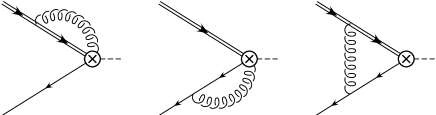
Figure 1: One-loop diagrams for the calculation of the anomalous dimension of the $B$-meson light-cone distribution amplitude.

We may separate the on- and off-diagonal terms of the anomalous dimension and express it as

$$\gamma_{+}(\omega,\omega^{\prime},\mu) = \Big{[}\Gamma_{cusp}(\alpha_{s})\ln\frac{\mu}{\omega}+\gamma(\alpha_{s})\Big{]}\delta(\omega-\omega^{\prime})$$ (5)

$$+\omega\;\Gamma(\omega,\omega^{\prime},\alpha_{s})$$

to all orders in perturbation theory. The cusp anomalous dimension $\Gamma_{cusp}(\alpha_{s})$ appears as the coefficient of the $\ln\mu$ term and has a geometric origin Korchemsky:wg : Since an effective heavy-quark field $h(0)$ can be expressed as the product of a free field and a Wilson line $S_{v}(0,-\infty)$ extending from $(-\infty)$ to $0$ along the $v$-direction, the matrix element in (1) contains $S_{n}(z,0)\,S_{v}(0,-\infty)$ which can be combined to form a single Wilson line with a cusp at the origin, as shown in Fig. 2(a). The appearance of the single $\ln\mu$ term distinguishes the anomalous dimension of the $B$-meson LCDA from the familiar Brodsky-Lepage kernel Lepage:1980fj . On the one-loop level the $\ln\mu$ term appears in the calculation of the first diagram in Fig. 1, where the gluon from the Wilson line $S_{n}(z,0)$ connects to the heavy-quark Wilson line $S_{v}(0,-\infty)$.

We find the one-loop expressions Lange:2003ff (denoted by the superscript ⁽¹⁾) to be $\Gamma_{cusp}^{(1)}=4$, $\gamma^{(1)}=-2$, and

$$\Gamma^{(1)}(\omega,\omega^{\prime})=-\Gamma_{cusp}^{(1)}\left[\frac{\theta(\omega^{\prime}-\omega)}{\omega^{\prime}(\omega^{\prime}-\omega)}+\frac{\theta(\omega-\omega^{\prime})}{\omega(\omega-\omega^{\prime})}\right]_{+}\;,$$ (6)

where we have used that $\gamma_{F}^{(1)}=-3$ is the one-loop coefficient of the anomalous dimension of heavy-to-light currents. The subscript $+$ denotes the standard “plus distribution” which ensures that $\int d\omega^{\prime}\Gamma(\omega,\omega^{\prime})=0$.

3 Keys to the exact solution

The first key toward solving the RG Eq. (4) concerns the off-diagonal term $\omega\Gamma(\omega,\omega^{\prime},\mu)$ in the anomalous dimension (5). We observe that (omitting $\alpha_{s}\equiv\alpha_{s}(\mu)$ dependence)

$$\int\limits_{0}^{\infty}d\omega^{\prime}\omega\Gamma(\omega,\omega^{\prime})(\omega^{\prime})^{a}=\omega^{a}{\mathcal{F}}(a)$$ (7)

on dimensional grounds. The dimensionless function ${\mathcal{F}}$ can only depend on the (in general complex) exponent $a(\mu)$, which in turn must be allowed to depend on the renormalization scale $\mu$. We can therefore use a power-law ansatz

$$f(\omega,\mu,\mu_{0},a(\mu))=\left(\frac{\omega}{\mu_{0}}\right)^{a(\mu)}\;e^{U(a(\mu),\mu)}$$ (8)

with an arbitrary mass parameter $\mu_{0}$. The function $f$ solves the RG Eq. (4), if the exponent $a(\mu)$ and the normalization $U(a(\mu),\mu)$ obey the differential equations

$$\frac{d}{d\ln\mu}\,a(\mu) = \Gamma_{cusp}(\alpha_{s})\;,$$ (9)

$$\frac{d\,U(a(\mu),\mu)}{d\ln\mu}\, = -\gamma(\alpha_{s})-{\mathcal{F}}(a(\mu),\alpha_{s})-\ln\frac{\mu}{\mu_{0}}\,\Gamma_{cusp}(\alpha_{s})\;.$$

The first equation can be immediately integrated and yields $a(\mu)=\eta+g(\mu,\mu_{0})$ with initial value $\eta=a(\mu_{0})$ and

$$g(\mu,\mu_{0})=\int\limits_{\alpha_{s}(\mu_{0})}^{\alpha_{s}(\mu)}\frac{d\alpha}{\beta(\alpha)}\;\Gamma_{cusp}(\alpha)\;.$$ (10)

With this solution at hand, the second equation integrates to

$$U(a(\mu),\mu) = -\int\limits_{\alpha_{s}(\mu_{0})}^{\alpha_{s}(\mu)}\frac{d\alpha}{\beta(\alpha)}\;\Big{[}\gamma(\alpha)+g_{\mu}(\alpha)$$ (11)

$$\hskip 56.9055pt+{\mathcal{F}}(\eta+g_{0}(\alpha),\alpha)\Big{]}\;,$$

where $g_{\mu}(\alpha)=g(\mu,\mu_{\alpha})$, $g_{0}(\alpha)=g(\mu_{\alpha},\mu_{0})$, and $\mu_{\alpha}$ is defined such that $\alpha_{s}(\mu_{\alpha})=\alpha$. Note that $g(\mu_{0},\mu_{0})=0$ and $U(\eta,\mu_{0})=0$ in this construction.

The second key to the solution concerns the initial condition $\phi_{+}^{B}(\omega,\mu_{0})$. Defining the Fourier transform $\varphi_{0}(t)$ of the LCDA at scale $\mu_{0}$ with respect to $\ln(\omega/\mu_{0})$ allows us to express the $\omega$ dependence in the desired power-law form

$$\phi_{+}^{B}(\omega,\mu_{0})=\frac{1}{2\pi}\int\limits_{-\infty}^{\infty}dt\;\varphi_{0}(t)\left(\frac{\omega}{\mu_{0}}\right)^{it}\;.$$ (12)

We therefore obtain an exact analytic expression for the solution of the RG Eq. (4) as the single integral

$$\phi_{+}^{B}(\omega,\mu)=\frac{1}{2\pi}\int\limits_{-\infty}^{\infty}dt\;\varphi_{0}(t)\;f(\omega,\mu,\mu_{0},\eta=it)\;.$$ (13)

4 Asymptotic behaviour

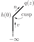
(a)           (b)

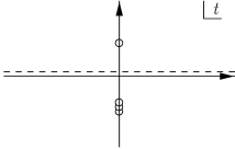
Figure 2: (a) Left: The cusp in the Wilson line $S_{n}(z,0)S_{v}(0,-\infty)$. (b) Right: Poles of the function $f(\ldots,it)$ in the complex $t$ plane. The upper pole remains stationary under renormalization flow, whereas the position of the lower pole moves toward the real axis for increasing $\mu$.

The solution (13) enables us to extract the asymptotic behaviour of the LCDA $\phi_{+}^{B}(\omega,\mu)$ as $\omega\to 0$ and $\omega\to\infty$ by deforming the integration contour in the complex $t$ plane. We hence need to study the analytic structure of the integrand $\varphi_{0}(t)\;f(\omega,\mu,\mu_{0},it)\sim\omega^{it+g(\mu,\mu_{0})}$. If $\omega$ is very small we can deform the contour into the lower half plane and then the position of the nearest pole to the real axis determines the $\omega$ dependence of $\phi_{+}^{B}(\omega,\mu)$. Similarly the nearest pole in the upper half plane dominates for very large $\omega$.

Let us study the analytic structure of $f(\omega,\mu,\mu_{0},it)$ at leading order in RG-improved perturbation theory. Using the one-loop expressions (6) and the definition (7) we find

$${\mathcal{F}}^{(1)}(a)=\Gamma_{cusp}^{(1)}\left[\Psi(1+a)+\Psi(1-a)+2\gamma_{E}\right]\;.$$ (14)

$\Psi$ and $\gamma_{E}$ denote the logarithmic derivative of the Euler-Gamma function and the Euler-constant, respectively. Plugging this result into eq. (11) with $\eta=it$ one obtains (using the short-hand notation $g\equiv g(\mu,\mu_{0})$)

$$e^{U(it+g,\mu)}\propto\frac{\Gamma(1+it)\;\Gamma(1-it-g)}{\Gamma(1-it)\;\Gamma(1+it+g)}\;.$$ (15)

The function $f(\omega,\mu,\mu_{0},it)$ has poles along the imaginary axis, and the closest to the real axis are located at $t=i$ and $t=-i(1-g)$. Using the one-loop expression (10) we observe that the function $g$ vanishes at $\mu=\mu_{0}$ by definition and grows monotonously as $\mu$ increases. Therefore the position of the pole in the lower complex plane approaches the real axis under renormalization evolution, as illustrated in Fig. 2(b).

These poles “compete” with the singularities arising from $\varphi_{0}(t)$ for the nearest position to the real axis. Let us assume that, for a given model of $\phi_{+}^{B}(\omega,\mu_{0})$, the LCDA grows like $\omega^{\delta}$ for small $\omega$ and falls off like $\omega^{-\xi}$ for large $\omega$. The corresponding poles of the function $\varphi_{0}(t)$ are then located at $t=-i\delta$ and $t=i\xi$. We therefore obtain the asymptotic behaviour of the renormalized LCDA as

$$\phi_{+}^{B}(\omega,\mu)\sim\cases{\omega^{\min(1,\delta+g)}\,;&for $\omega\to 0$,\cr\omega^{-\min(1,\xi)+g}\,;&for $\omega\to\infty$.\cr}$$ (16)

The two immediate observations are that, regardless of how small the value of $\delta$ is, evolution effects will drive the small $\omega$ behaviour toward linear growth, and that the renormalized LCDA at a scale $\mu>\mu_{0}$ will fall off slower than $1/\omega$ irrespective of how fast it vanishes at $\mu=\mu_{0}$.

5 Concluding Remarks

The emergence of a radiative tail after (even infinitesimally small) evolution seems, at first sight, a very strange property of the LCDA, because it implies that the normalization integral of $\phi_{+}^{B}(\omega,\mu)$ is UV divergent. This can be understood as the corresponding local operator $\tilde{\phi}_{+}^{B}(\tau=0,\mu)$ requires an additional subtraction when renormalized. However, this is not an obstacle in practical applications in which only $\phi_{+}^{B}(\omega,\mu)/\omega$ modulo logarithms appears. An integral over this function remains UV finite as long as $g(\mu,\mu_{0})<1$, at which point the pole at $t=-i(1-g)$ reaches the real axis and the above formalism breaks down.

It is evident from (16) that evolution effects mix different moments of the LCDA. For example, the first inverse moment of $\phi_{+}^{B}(\omega,\mu)$ defines a parameter $\lambda_{B}(\mu)$,

$$\frac{1}{\lambda_{B}(\mu)}=\int\limits_{0}^{\infty}\frac{d\omega}{\omega}\;\phi_{+}^{B}(\omega,\mu)\;,$$ (17)

which is connected to a fractional inverse moment of order $1-g(\mu,\mu^{\prime})$ at a different scale $\mu^{\prime}$. This makes it impossible to calculate the scale dependence of $\lambda_{B}(\mu)$ in perturbation theory without knowledge of the LCDA.

In this talk I presented the renormalization-group equation of the $B$-meson LCDA and discussed the key steps in solving this integro-differential equation analytically. Since the amplitude (2) is independent of the renormalization scale $\mu$, the technique presented here can be used to resum Sudakov logarithms in the hard scattering kernel $T(\omega,\mu)$, which was demonstrated in reference Bosch:2003fc for the $B\to\gamma l\nu$ decay mode.

Let me stress that the solution outlined here can also be used in other applications in $B$-physics, such as the the inclusive $B\to X_{s}\gamma$ for example, in which the shape-function and the hard-scattering kernel relevant to the analysis of the photon spectrum Neubert:1993um ; Bauer:2000ew obey evolution equations similar to (4).

Acknowledgments

I would like to thank T. Mannel for lunch and an interesting discussion.

References

-
(1)
M. Beneke, G. Buchalla, M. Neubert and C. T. Sachrajda,
Phys. Rev. Lett. 83, 1914 (1999)
[hep-ph/9905312];
Nucl. Phys. B 591, 313 (2000) [hep-ph/0006124];
Nucl. Phys. B 606, 245 (2001) [hep-ph/0104110]. - (2) A. G. Grozin and M. Neubert, Phys. Rev. D 55, 272 (1997) [hep-ph/9607366].
- (3) B. O. Lange and M. Neubert, “Renormalization-group evolution of the B-meson light-cone distribution amplitude,” Phys. Rev. Lett. 91, 102001 (2003) [arXiv:hep-ph/0303082].
- (4) S. W. Bosch, R. J. Hill, B. O. Lange and M. Neubert, preprint hep-ph/0301123.
- (5) G. P. Korchemsky and A. V. Radyushkin, Nucl. Phys. B 283, 342 (1987); I. A. Korchemskaya and G. P. Korchemsky, Phys. Lett. B 287, 169 (1992).
- (6) G. P. Lepage and S. J. Brodsky, Phys. Rev. D 22, 2157 (1980).
- (7) M. Neubert, Phys. Rev. D 49, 4623 (1994) [arXiv:hep-ph/9312311].
- (8) C. W. Bauer, S. Fleming and M. E. Luke, Phys. Rev. D 63, 014006 (2001) [arXiv:hep-ph/0005275].