Radiative Corrections to One-Photon Decays of Hydrogenic Ions

Abstract

Radiative corrections to the decay rate of $n=2$ states of hydrogenic ions are calculated. The transitions considered are the M1 decay of the $2s$ state to the ground state and the E1(M2) decays of the $2p_{1/2}$ and $2p_{3/2}$ states to the ground state. The radiative corrections start in order $\alpha(Z\alpha)^{2}$, but the method used sums all orders of $Z\alpha$. The leading $\alpha(Z\alpha)^{2}$ correction for the E1 decays is calculated and compared with the exact result. The extension of the calculational method to parity nonconserving transitions in neutral atoms is discussed.

I Introduction

Radiative corrections to decay rates in atoms and ions have not been as thoroughly studied as other kinds of radiative corrections, such as the Lamb shift PJM and corrections to hyperfine splitting (hfs) hfs1 ; hfs2 . An exception is the case of the exotic atom positronium, where differences between the lowest-order decay rates and experiment of -0.6 and -2.2 percent are present for parapositronium paraexp and orthopositronium orthoexp , respectively. In both cases the bulk of the difference is accounted for by one-loop radiative corrections Harris-Brown ; Lepage , which enter in order $\alpha$ with large coefficients, and the present theoretical interest has advanced to the level of two-loop radiative corrections CMY ; AFS .

For other hydrogenlike atoms, theoretical work on one-loop corrections to M1 decays has been carried out in Ref. Lin-Feinberg ; Barbieri-Sucher . These papers established that, unlike positronium, the order $\alpha$ correction has a vanishing coefficient, but did not calculate the actual correction, which enters in order $\alpha(Z\alpha)^{2}$. A calculation for E1 decays of the $\alpha(Z\alpha)^{2}\ln(Z\alpha)$ correction has been carried out in Ref. Ivanov , and is in disagreement with another calculation associated with the experimental determination of the Lamb shift Sok . This situation will be discussed further in the conclusion.

It is the purpose of the present paper to calculate radiative corrections for the hydrogen isoelectronic sequence using methods that treat the electron propagator exactly. In addition, a perturbative calculation for E1 decays through order $\alpha(Z\alpha)^{2}$ is carried out and compared to the exact result. While of intrinsic interest, development of these techniques should also aid in the evaluation of radiative corrections to parity nonconserving transitions in atoms, as will be discussed in the conclusion.

II Lowest-order calculation

While the first calculations of the decay rate of hydrogen date back to the beginning of quantum mechanics, fully relativistic calculations needed for calculations of highly-charged hydrogenlike ions were first carried out in the early 1970’s Drakeh . We briefly present the theory here using techniques that will be extended to the radiative correction case. We want to use the fact that a decay rate can be related to the imaginary part of the energy through

$$\Gamma=-2\,\Im(E).$$ (1)

This is the approach taken by Barbieri and Sucher Barbieri-Sucher . The one-photon decay rate is connected through this formula with the self-energy of an electron in a state $v$, which will be chosen here to be $2s_{1/2}$, $2p_{1/2}$, or $2p_{3/2}$. We define this self-energy as $\Sigma_{vv}(\epsilon_{v})$, where

$$\Sigma_{ml}(E)=-ie^{2}\!\int\!d^{3}x\,d^{3}y\!\int\!{d^{n}k\over(2\pi)^{n}}\,{e^{i\vec{k}\cdot(\vec{x}-\vec{y})}\over k^{2}+i\delta}\,\bar{\psi}_{m}(\vec{x})\gamma_{\mu}S_{F}(\vec{x},\vec{y};E-k_{0})\gamma^{\mu}\psi_{l}(\vec{y}),$$ (2)

and a self-mass counterterm needed to renormalize $\Sigma$ is understood to be included. If we set $n=4$, carry out the $d^{3}k$ integration, and represent the Dirac-Coulomb propagator by a spectral decomposition, the above can be written

$$\Sigma_{ml}(E)=i\alpha\!\int\!d^{3}x\,d^{3}y\!\int\!{dk_{0}\over 2\pi}\sum_{r}{e^{i\sqrt{k_{0}^{2}+i\delta}\,|\vec{x}-\vec{y}|}\over|\vec{x}-\vec{y}|}{\bar{\psi}_{m}(\vec{x})\gamma_{\mu}\psi_{r}(\vec{x})\,\bar{\psi}_{r}(\vec{y})\gamma^{\mu}\psi_{l}(\vec{y})\over E-k_{0}-\epsilon_{r}(1-i\delta)}.$$ (3)

If we define

$$g_{ijkl}(E)=\alpha\!\int\!d^{3}x\,d^{3}y\,{e^{i\sqrt{E^{2}+i\delta}\,|\vec{x}-\vec{y}|}\over|\vec{x}-\vec{y}|}\,\bar{\psi}_{i}(\vec{x})\gamma_{\mu}\psi_{k}(\vec{x})\,\bar{\psi}_{j}(\vec{y})\gamma^{\mu}\psi_{l}(\vec{y}),$$ (4)

then the self-energy can be compactly represented as

$$\Sigma_{vv}(\epsilon_{v})=i\!\int\!{dk_{0}\over 2\pi}\sum_{m}{g_{vmmv}(k_{0})\over\epsilon_{v}-k_{0}-\epsilon_{m}(1-i\delta)}.$$ (5)

It will be convenient below to also introduce the function

$$\bar{g}_{ijkl}(E)=\alpha\!\int\!d^{3}x\,d^{3}y\,{\sin(E|\vec{x}-\vec{y}|)\over|\vec{x}-\vec{y}|}\,\bar{\psi}_{i}(\vec{x})\gamma_{\mu}\psi_{k}(\vec{x})\,\bar{\psi}_{j}(\vec{y})\gamma^{\mu}\psi_{l}(\vec{y}).$$ (6)

To carry out the numerical evaluation of the Lamb shift, a Wick rotation with $k_{0}\rightarrow i\omega$ is performed. The resulting expression is purely real because imaginary parts present in the $\omega=0-\infty$ interval cancel against other imaginary parts in the $\omega=\text{-}\infty-0$ interval. The imaginary part of the self-energy arises solely from the pole term, where a bound state pole in the first quadrant present when $\epsilon_{v}>\epsilon_{m}$ is encircled during the Wick rotation. As we are interested in decays to the ground state, we will not consider imaginary parts of the energy arising from $m$ being an excited state in Eq. (5). We introduce the convention that $a$ refers to the ground state when there is no dependence on the magnetic quantum number (as is the case for the energy $\epsilon_{a}$ and the self-energy $\Sigma_{aa}(\epsilon_{a})$), and $b$ or $c$ refers to the ground state when there is a dependence, with a sum over $b$ or $c$ running over the two possible values ($\pm 1/2$) of the magnetic quantum number. We also define the lowest-order decay photon energy $\Delta E=\epsilon_{v}-\epsilon_{a}$. It is important to emphasize that this energy differs from the actual photon energy because the energy levels are shifted by radiative corrections: the effect of these shifts will be accounted for perturbatively below. The pole term is

$$\Sigma_{\rm pole}=\sum_{b}g_{vbbv}(\Delta E).$$ (7)

In calculations of the Lamb shift the real part of this is taken, but here we are concerned with the imaginary part, which gives the lowest-order decay rate

$$\Gamma_{0}=-2\sum_{b}\bar{g}_{vbbv}(\Delta E),$$ (8)

which can be written as a partial wave expansion

$$\Gamma_{0}=-8\pi\alpha\Delta E \!\!\!\sum_{blm}\int\!d^{3}x\,j_{l}(\Delta Ex)Y_{lm}(\Omega_{x})\,\bar{\psi}_{v}(\vec{x})\gamma_{\mu}\psi_{b}(\vec{x})$$ (9)

$$\times\int\!d^{3}y\,j_{l}(\Delta Ey)Y^{*}_{lm}(\Omega_{y})\,\bar{\psi}_{b}(\vec{y})\gamma^{\mu}\psi_{v}(\vec{y}).$$

Because Feynman gauge has been used for the self-energy calculation, this form of the decay rate is different from derivations which use the properties of the actual transverse photons that are emitted, but the result is the same because of gauge invariance. In Table 1, we present the lowest-order rates for the states $2s_{1/2}$, $2p_{1/2}$, and $2p_{3/2}$ to decay by one-photon emission to the ground state for $Z=5,10,\ldots,100$. We now turn to the radiative corrections to these decay rates, which we define in terms of a function $R(Z\alpha)$,

$$\Gamma=\Gamma_{0}\,\Big{[}1+{\alpha\over\pi}\,R(Z\alpha)\Big{]}.$$ (10)

Before presenting the exact calculation of $R(Z\alpha)$, we calculate the leading contribution of order $(Z\alpha)^{2}$ for the $p$ states using an effective field theory approach. We do not treat the more complicated $s$ state correction, as the M1 decay is highly suppressed at low $Z$.

III Perturbative Approach

When $Z$ is small, an expansion in $Z\alpha$ converges rapidly. We present here the calculation of $R(Z\alpha)$ to leading order $(Z\alpha)^{2}$, which will serve as a check of the nonperturbative treatment presented in the next section. The radiative correction to the decay rate is obtained from the nonrelativistic form of quantum electrodynamics (QED) supplemented by one-loop corrections to electron form factors $F_{1}$, $F_{2}$ and the vacuum polarization. In the lowest order, the decay rate of the $2P$ state in hydrogen-like atoms is

$$\Gamma_{0}=\frac{4}{9}\,\alpha E^{3}\left|\langle 1S\,|\vec{r}\,|2\vec{P}\,\rangle\right|^{2},$$ (11)

where $E$ is the nonrelativistic limit of $\Delta E$ defined in the previous section,

$$E=E(2P)-E(1S)={3m(Z\alpha)^{2}\over 8},$$ (12)

with the nonrelativistic wave functions

$$\phi_{1S} = \frac{1}{\sqrt{4\pi}}\,(mZ\alpha)^{3/2}\,2e^{-mZ\alpha r},$$ (13)

$$\vec{\phi}_{2P} = \frac{1}{\sqrt{4\pi}}\,\frac{1}{2\sqrt{6}}\,(mZ\alpha)^{3/2}\,e^{-mZ\alpha r/2}\,(mZ\alpha\vec{r}).$$ (14)

Natural units in which $\hbar=c=1$ are used here. Note that $\vec{\phi}_{2P}$ is normalized here in a nonstandard way, namely $\int d^{3}r\,\vec{\phi}_{2P}\cdot\vec{\phi}_{2P}=1$. Using the nonrelativistic matrix element

$$d\equiv\langle 1S\,|\vec{r}\,|2\vec{P}\,\rangle=\frac{1}{\sqrt{6}}\,\frac{256}{81}\,{1\over mZ\alpha},$$ (15)

Eq. (11) gives the well-known decay rate

$$\Gamma_{0}={2^{8}\over 3^{8}}\,m\alpha(Z\alpha)^{4}.$$ (16)

The radiative corrections to this can be expressed as

$${\alpha\over\pi}\,R\equiv\frac{\delta\Gamma}{\Gamma_{0}}=3\,\frac{\delta E}{E}+2\,\frac{\delta d}{d}\,.$$ (17)

When QED effects can be treated as local potentials, the calculation of radiative corrections is relatively simple. We illustrate this with the correction due to the presence of vacuum polarization, which is given in the nonrelativistic limit by a local interaction potential

$$\delta V=-{4Z\alpha^{2}\over 15m^{2}}\,\delta^{3}(\vec{r}).$$ (18)

Corrections to the energy and wave function of the $2P$ state from $\delta V$ do not contribute to $R(Z\alpha)$ at the order of interest, but the potential shifts the $1S$ energy by

$$\delta E(1S)=-{4m\alpha(Z\alpha)^{4}\over 15\pi},$$ (19)

which gives a contribution to $R(Z\alpha)$ of $32/15\,(Z\alpha)^{2}$. In addition the potential shifts the $1S$ wave function by

$$\delta\phi_{1S} \equiv \bigg{\langle}r\,\bigg{|}\frac{1}{(E-H)^{\prime}}\,\delta V\,\bigg{|}1S\bigg{\rangle}$$ (20)

$$= {8\alpha(Z\alpha^{2})\over 15\pi}\,e^{-mZ\alpha r}\bigg{[}{5\over 2}-\gamma_{E}-mZ\alpha r+{1\over 2mZ\alpha r}-\ln(2mZ\alpha r)\bigg{]}{1\over\sqrt{4\pi}}(mZ\alpha)^{3/2},~{}~{}$$

which leads to a total contribution from vacuum polarization of

$$R_{\rm VP}(Z\alpha) = (Z\alpha)^{2}\,\biggl{\{}{32\over 15}+\biggl{[}-{8\over 15}\ln{4\over 3}-{131\over 90}\biggr{]}\biggr{\}}$$ (21)

$$= (Z\alpha)^{2}\,\biggl{[}{61\over 90}-{8\over 15}\ln{4\over 3}\biggr{]}$$

$$= (Z\alpha)^{2}\;\Bigl{[}\,0.524\;347\,\Bigr{]}.$$

We note the strong cancellation between the effect of the energy shift, which is automatically accounted for when experimental energies are used, and the perturbed orbital, which shows care needs to be taken when that approach is taken. We now turn to the more complex self-energy correction. The effect on the energy shift is well-known, coming from the self-energy part of the Lamb shift of the $1S$ and $2P_{1/2}$ states of

$$\delta E(1S) = \frac{m\alpha}{\pi}\,(Z\alpha)^{4}\,\biggl{[}\frac{10}{9}+\frac{4}{3}\ln(Z\alpha)^{-2}-\frac{4}{3}\ln k_{0}(1S)\biggr{]},$$ (22)

$$\delta E(2P) = \frac{m\alpha}{\pi}\,(Z\alpha)^{4}\,\frac{1}{8}\,\biggl{[}-\frac{1}{6}-\frac{4}{3}\ln k_{0}(2P)\biggr{]},$$ (23)

where

$$\ln k_{0}(1S) = 2.984\;128\;556\,,$$ (24)

$$\ln k_{0}(2P) = -0.030\;016\;709\,.$$ (25)

This energy shift contributes to the decay rate in accordance with Eq. (17). However, the radiative corrections to the dipole matrix element are more difficult to obtain. We split this correction into three parts, $\delta d=\delta d_{L}+\delta d_{H}+\delta d_{K}$, where $\delta d_{L}$ comes from low-energy photons, $\delta d_{H}$ is the high-energy correction to the wave function, and $\delta d_{K}$ is the correction to the dipole operator. Using nonrelativistic QED one derives the following expression for $\delta d_{L}$

$$\delta d_{L} = \frac{2\alpha}{3\pi m^{2}}\int_{0}^{\epsilon}\!\omega\,d\omega\,\Re[f(\omega)]\,,$$ (26)

$$f(\omega) = \biggl{\langle}S\,\biggl{|}\,p_{i}\,\frac{1}{H-E_{S}+\omega}\,r_{j}\,\frac{1}{H-E_{P}+\omega}\,p_{i}\,\biggr{|}P_{j}\biggr{\rangle}$$ (27)

$$+\,\biggl{\langle}S\,\biggl{|}\,r_{j}\,\frac{1}{(H-E_{P})^{\prime}}\,p_{i}\,\frac{1}{H-E_{P}+\omega}\,p_{i}\,\biggr{|}P_{j}\biggr{\rangle}$$

$$+\,\biggl{\langle}S\,\biggl{|}\,p_{i}\,\frac{1}{H-E_{S}+\omega}\,p_{i}\,\frac{1}{(H-E_{S})^{\prime}}\,r_{j}\,\biggr{|}P_{j}\biggr{\rangle}$$

$$-\,\frac{d}{2}\,\biggl{\langle}S\,\biggl{|}\,p_{i}\,\frac{1}{(H-E_{S}+\omega)^{2}}\,p_{i}\,\biggr{|}S\biggr{\rangle}$$

$$-\,\frac{d}{2}\,\biggl{\langle}P_{j}\,\biggl{|}\,p_{i}\,\frac{1}{(H-E_{P}+\omega)^{2}}\,p_{i}\,\biggr{|}P_{j}\biggr{\rangle}\,,$$

where $\epsilon$ is assumed to be asymptotically large and $i$, $j$ are vector coordinate indices. All matrix elements of $f(\omega)$ are calculated numerically using a finite difference representation of the nonrelativistic Hamiltonian. The integration with respect to $\omega$ requires special treatment regarding linear and logarithmic in $\epsilon$ terms. The large $\omega$ asymptotics is

$$f(\omega)\approx\frac{A}{\omega}+\frac{B}{\omega^{2}}+\frac{C}{\omega^{5/2}}+\ldots$$ (28)

where

$$A = \biggl{\langle}S\,\biggl{|}\,p^{2}\,\frac{1}{(H-E_{S})^{\prime}}\,r_{i}\,\biggr{|}P_{i}\biggr{\rangle}\,+\,\biggr{\langle}S\,\biggl{|}\,r_{i}\,\frac{1}{(H-E_{P})^{\prime}}\,p^{2}\,\biggr{|}P_{i}\biggr{\rangle}=-2d$$ (29)

$$B = -\frac{1}{2}\,\biggl{\langle}S\,\biggl{|}\,4\pi Z\alpha\,\delta^{3}(r)\,\frac{1}{(H-E_{S})^{\prime}}\,r_{i}\,\biggr{|}P_{i}\biggr{\rangle}=d\,(Z\alpha)^{2}\,\biggl{(}\frac{131}{24}+2\ln\frac{4}{3}\biggr{)},$$ (30)

$$C = 2\sqrt{2}B\,(Z\alpha).$$ (31)

The numerical integration in Eq. (26), along a contour which omits poles from above or below, leads to the result

$$\delta d_{L}=\frac{2\alpha}{3\pi}\,\biggl{\{}A\epsilon+B\ln\biggl{[}\frac{2\epsilon}{(Z\alpha)^{2}}\biggr{]}-d\,(Z\alpha)^{2}\,17.759\;359\biggr{\}}\,.$$ (32)

The term linear in $\epsilon$ is dropped, and the logarithmic term is canceled by the contribution $\delta d_{H}$ coming from large photon momenta. This latter contribution can be expressed in terms of an interaction potential $\delta V$ obtained from the one-loop electron form factors $F_{1}$ and $F_{2}$,

$$\delta V=Z\alpha^{2}\biggl{[}\frac{10}{9}-\frac{4}{3}\ln(2\epsilon)\biggr{]}\delta^{3}(r)+\frac{Z\alpha^{2}}{2\pi}\,\frac{\vec{L}\cdot\vec{S}}{r^{3}}\,.$$ (33)

It contributes to the energy shift in a way that has already been accounted for in Eqs. (22, 23), but also gives corrections to the wave functions, and thus to the transition dipole moment

$$\delta d_{H} = Z\alpha^{2}\biggl{[}\frac{10}{9}-\frac{4}{3}\ln(2\epsilon)\biggr{]}\biggl{\langle}S\,\biggl{|}\delta^{3}(r)\,\frac{1}{(E_{S}-H)^{\prime}}\,\vec{r}\,\biggr{|}\vec{P}\biggr{\rangle}$$ (34)

$$+\,\frac{Z\alpha^{2}}{2\pi}\,\biggl{\langle}S\,\biggl{|}\,\vec{r}\,\frac{1}{(E_{P}-H)^{\prime}}\,\frac{\vec{L}\cdot\vec{S}}{r^{3}}\,\biggr{|}\vec{P}\biggr{\rangle}.$$

There is one more spin-dependent term which recently was discussed in Ref. forbidden . It arises from the anomalous magnetic moment $\kappa$ correction to the dipole transition operator

$$i\,\omega\,\vec{r}-\frac{\kappa}{4\,m}\,\vec{k}^{2}\,\vec{r}\times\vec{\sigma}.$$ (35)

Its matrix element between $S$ and $P_{1/2}$ states leads to a correction $\delta d_{K}$

$$\delta d_{K}=-d\,\frac{E\,\kappa}{4\,m}\,2=-d\,\frac{3\,\alpha}{32\,\pi}\,(Z\,\alpha)^{2}.$$ (36)

With the help of Eq. (17), the sum $\delta d_{L}+\delta d_{H}+\delta d_{K}$, together with energy shift contributions from Eqs. (22, 23), leads finally to the result for the radiative correction to the decay rate of the $2P_{1/2}$ state

$$R_{\rm SE}^{2p_{1/2}}(Z\alpha)=(Z\alpha)^{2}\biggl{\{}\biggl{[}{8\over 3}\,\ln{4\over 3}-{61\over 18}\biggr{]}\!\ln(Z\alpha)^{-2}+6.051~{}68\biggr{\}}.$$ (37)

A similar calculation for the $2P_{3/2}$ state yields

$$R_{\rm SE}^{2p_{3/2}}(Z\alpha)=(Z\alpha)^{2}\biggl{\{}\biggl{[}{8\over 3}\,\ln{4\over 3}-{61\over 18}\biggr{]}\!\ln(Z\alpha)^{-2}+5.984~{}36\biggr{\}}.$$ (38)

The coefficient of the logarithmic term is in agreement with Ivanov .

IV Two-loop formalism

Following the approach given above to calculate radiative corrections to decay rates, we consider the imaginary part of the two-loop Lamb shift. We begin by considering the three self-energy diagrams of Fig. 1, leaving vacuum polarization for later. Expressions for the diagrams, which we refer to as overlap, nested, and reducible following the notation of Fox and Yennie Fox-Yennie , were derived by Mills and Kroll Kroll-Mills , and we now treat them in order.

IV.1 Overlap diagram

The overlap diagram, Fig. 1a, is given by

$$\Sigma^{4O} = -e^{4}\!\int\!d^{3}x\,d^{3}y\,d^{3}z\,d^{3}w\!\int\!{d^{n}k\over(2\pi)^{n}}\,{d^{n}l\over(2\pi)^{n}}\,{e^{i\vec{k}\cdot(\vec{x}-\vec{z})}\over k^{2}+i\delta}\,{e^{i\vec{l}\cdot(\vec{y}-\vec{w})}\over l^{2}+i\delta}\,\bar{\psi}_{v}(\vec{x})\gamma^{\mu}$$ (39)

$$\times\,S_{F}(\vec{x},\vec{y};\epsilon_{v}-k_{0})\gamma^{\nu}S_{F}(\vec{y},\vec{z};\epsilon_{v}-k_{0}-l_{0})\gamma_{\mu}S_{F}(\vec{z},\vec{w};\epsilon_{v}-l_{0})\gamma_{\nu}\psi_{v}(\vec{w}).$$

As with the one-loop case, we introduce spectral representations for the electron propagators and carry out the $d^{3}k$ and $d^{3}l$ integrations to get

$$\Sigma^{4O}=-\sum_{mnr}\int{dk_{0}\over 2\pi}\int{dl_{0}\over 2\pi}\,{g_{vnmr}(k_{0})\,g_{mrnv}(l_{0})\over(\epsilon_{v}-k_{0}-\epsilon_{m})(\epsilon_{v}-k_{0}-l_{0}-\epsilon_{n})(\epsilon_{v}-l_{0}-\epsilon_{r})},$$ (40)

where in this section we leave the factor $(1-i\delta)$ multiplying energies in the spectral representation of the electron propagator understood. We now consider Wick rotating both $k_{0}\rightarrow i\omega_{k}$ and $l_{0}\rightarrow i\omega_{l}$. If no poles are passed, this again leads to a purely real expression. To get an imaginary part, at least one of the three denominators must involve encircling a pole. The middle denominator can have a pole when $n=a$ and $k_{0}+l_{0}=\Delta E$, but this corresponds to two-photon decay which we do not treat here. We then need consider only the two cases when either $m=a$ and $k_{0}=\Delta E$ or $r=a$ and $l_{0}=\Delta E$, which gives the expressions

$$\Sigma^{4O}_{L} = -4\pi i\alpha^{2}\sum_{b}\int\!d^{3}x\,d^{3}y\,d^{3}z\,d^{3}w\,{e^{i\Delta E|\vec{x}-\vec{z}|}\over|\vec{x}-\vec{z}|}\!\int\!{d^{n}l\over(2\pi)^{n}}\,{e^{i\vec{l}\cdot(\vec{y}-\vec{w})}\over l^{2}+i\delta}$$ (41)

$$\times\,\bar{\psi}_{v}(\vec{x})\gamma^{\mu}\psi_{b}(\vec{x})\,\bar{\psi}_{b}(\vec{y})\gamma^{\nu}S_{F}(\vec{y},\vec{z};\epsilon_{a}-l_{0})\gamma_{\mu}S_{F}(\vec{z},\vec{w};\epsilon_{v}-l_{0})\gamma_{\nu}\psi_{v}(\vec{w})$$

and

$$\Sigma^{4O}_{R} = -4\pi i\alpha^{2}\sum_{b}\int\!d^{3}x\,d^{3}y\,d^{3}z\,d^{3}w\,{e^{i\Delta E|\vec{y}-\vec{w}|}\over|\vec{y}-\vec{w}|}\!\int\!{d^{n}k\over(2\pi)^{n}}\,{e^{i\vec{k}\cdot(\vec{x}-\vec{z})}\over k^{2}+i\delta}$$ (42)

$$\times\,\bar{\psi}_{v}(\vec{x})\gamma^{\mu}S_{F}(\vec{x},\vec{y};\epsilon_{v}-k_{0})\gamma^{\nu}S_{F}(\vec{y},\vec{z};\epsilon_{a}-k_{0})\gamma_{\mu}\psi_{b}(\vec{z})\,\bar{\psi}_{b}(\vec{w})\gamma_{\nu}\psi_{v}(\vec{w}),$$

where we have “undone” the spectral representations of the electron propagator and kept either the $d^{3}k$ or $d^{3}l$ integration.

We note at this point that these expressions are almost identical to expressions that arise in the treatment of screening corrections to the self-energy in lithiumlike ions (Eqs. (25, 27) in Ref. libi ), with the only difference being an overall minus sign and the fact that we are interested in the imaginary part here, while the real part was calculated in libi . We were able then, with only slight modifications, to use code developed for the screening corrections in lithiumlike ions for the present calculation. Replacing

$$e^{i\Delta E|\vec{y}-\vec{w}|}\rightarrow i\sin(\Delta E|\vec{y}-\vec{w}|)$$ (43)

and using the equality of the two terms gives the net result for the decay rate contribution from the overlap diagram we call $\Gamma_{V}$,

$$\Gamma_{V} = -16\pi\alpha^{2}\Im\sum_{b}\int\!d^{3}x\,d^{3}y\,d^{3}z\,d^{3}w\,{\sin(\Delta E|\vec{x}-\vec{z}|)\over|\vec{x}-\vec{z}|}\,\bar{\psi}_{v}(\vec{x})\gamma^{\mu}\psi_{b}(\vec{x})$$ (44)

$$\times\int\!{d^{n}k\over(2\pi)^{n}}\,{e^{i\vec{k}\cdot(\vec{y}-\vec{w})}\over k^{2}+i\delta}\,\bar{\psi}_{b}(\vec{y})\gamma^{\nu}S_{F}(\vec{y},\vec{z};\epsilon_{a}-k_{0})\gamma_{\mu}S_{F}(\vec{z},\vec{w};\epsilon_{v}-k_{0})\gamma_{\nu}\psi_{v}(\vec{w}).$$

IV.2 Nested diagram

The nested diagram, Fig. 1b, is given by

$$\Sigma^{4N} = -e^{4}\!\int\!d^{3}x\,d^{3}y\,d^{3}z\,d^{3}w\!\int\!{d^{n}k\over(2\pi)^{n}}\,{d^{n}l\over(2\pi)^{n}}\,{e^{i\vec{k}\cdot(\vec{x}-\vec{w})}\over k^{2}+i\delta}\,{e^{i\vec{l}\cdot(\vec{y}-\vec{z})}\over l^{2}+i\delta}\,\bar{\psi}_{v}(\vec{x})\gamma^{\mu}$$ (45)

$$\times\,S_{F}(\vec{x},\vec{y};\epsilon_{v}-k_{0})\gamma^{\nu}S_{F}(\vec{y},\vec{z};\epsilon_{v}-k_{0}-l_{0})\gamma_{\nu}S_{F}(\vec{z},\vec{w};\epsilon_{v}-k_{0})\gamma_{\mu}\psi_{v}(\vec{w}).$$

This leads to the expression

$$\Sigma^{4N}=-\sum_{mnr}\int{dk_{0}\over 2\pi}\int{dl_{0}\over 2\pi}\,{g_{vrmv}(k_{0})\,g_{mnnr}(l_{0})\over(\epsilon_{v}-k_{0}-\epsilon_{m})(\epsilon_{v}-k_{0}-l_{0}-\epsilon_{n})(\epsilon_{v}-k_{0}-\epsilon_{r})}.$$ (46)

We again consider Wick rotating both $k_{0}\rightarrow i\omega_{k}$ and $l_{0}\rightarrow i\omega_{l}$, which gives a real result if no poles are passed. To get an imaginary part, at least one of the three denominators must encircles a pole, and once again, we omit poles arising from the middle denominator, which correspond to two-photon decay. We therefore need to consider only the $k_{0}$ Wick rotation, which has poles when $k_{0}=\Delta E$ and either $m=a$ or $r=a$. However, if both $m$ and $r$ are the ground state, a double pole is encountered. If the double pole is excluded, two terms result,

$$\Sigma^{4N}_{L}=\sum_{br}^{r\neq a}{g_{vrbv}(\Delta E)\Sigma_{br}(\epsilon_{a})\over\epsilon_{a}-\epsilon_{r}}\,,$$ (47)

and

$$\Sigma^{4N}_{R}=\sum_{bm}^{m\neq a}{g_{vbmv}(\Delta E)\Sigma_{mb}(\epsilon_{a})\over\epsilon_{a}-\epsilon_{m}}\,.$$ (48)

These terms can be written in terms of perturbed orbitals. Specifically, if we define

$$\tilde{\psi}_{a}(\vec{z})\equiv\sum_{br}^{r\neq a}\psi_{r}(\vec{z})\,{g_{vrbv}(\Delta E)\over\epsilon_{a}-\epsilon_{r}}\,\delta_{m_{b}m_{r}},$$ (49)

and

$$\tilde{\bar{\psi}}_{a}(\vec{z})\equiv\sum_{bm}^{m\neq a}\bar{\psi}_{m}(\vec{z})\,{g_{vbmv}(\Delta E)\over\epsilon_{a}-\epsilon_{m}}\,\delta_{m_{b}m_{m}},$$ (50)

then

$$\Sigma^{4N}_{L}+\Sigma^{4N}_{R}=\Sigma_{a\tilde{a}}(\epsilon_{a})+\Sigma_{\tilde{a}a}(\epsilon_{a}).$$ (51)

Because the ground state self-energy is purely real, the only contribution to the decay rate comes from the imaginary part of these perturbed orbital terms.

To treat the double pole, we set $m=b$ and $r=c$, and find

$$\Sigma^{4N}_{D}=i\sum_{bc}\int{dk_{0}\over 2\pi}\,{g_{vcbv}(k_{0})\Sigma_{bc}(\epsilon_{v}-k_{0})\over(\Delta E-k_{0}+i\delta)^{2}}\,.$$ (52)

Applying Cauchy’s theorem and using the fact that the self-energy is diagonal in magnetic quantum numbers gives two derivative terms,

$$\Sigma^{4N}_{D}=-\sum_{b}g^{\prime}_{vbbv}(\Delta E)\Sigma_{aa}(\epsilon_{a})+\sum_{b}g_{vbbv}(\Delta E){\Sigma^{\prime}}_{\!\!aa}(\epsilon_{a}).$$ (53)

IV.3 One-Particle Reducible Diagram

The final contribution to the two-loop self-energy comes from Fig. 1c, which breaks into two parts, a perturbed orbital term

$$\Sigma_{PO}=\sum_{m\neq v}{\Sigma_{vm}(\epsilon_{v})\Sigma_{mv}(\epsilon_{v})\over\epsilon_{v}-\epsilon_{m}},$$ (54)

and a derivative term

$$\Sigma_{D}=\Sigma_{vv}(\epsilon_{v})\,{\partial\Sigma_{vv}(E)\over\partial E}\,\Bigg{|}_{E=\epsilon_{v}}.$$ (55)

The perturbed orbital term will have an imaginary part only if at least one pole term is present, as our analysis of the complex nature of $\Sigma$ did not depend on the external wavefunctions, so long as they are real. This then leads to an imaginary contribution to the energy of

$$\Sigma_{PO}(a)=i[\Sigma_{v\tilde{v}}(\epsilon_{v})+\Sigma_{\tilde{v}v}(\epsilon_{v})],$$ (56)

where

$$\tilde{\psi}_{v}(\vec{z})\equiv\sum_{br}^{r\neq v}\psi_{r}(\vec{z})\,{\bar{g}_{vrbv}(\Delta E)\over\epsilon_{v}-\epsilon_{r}}\,,$$ (57)

and

$$\tilde{\bar{\psi}}_{v}(\vec{z})\equiv\sum_{bm}^{m\neq v}\bar{\psi}_{m}(\vec{z})\,{\bar{g}_{vbmv}(\Delta E)\over\epsilon_{v}-\epsilon_{m}}\,.$$ (58)

The derivative term will lead to an imaginary part of the energy in two ways: in the first, we take the imaginary part of the first self-energy, which is of course associated with the lowest-order decay rate, and multiply it by the real part of the derivative of the valence self-energy. We combine this term with the first term of Eq. (53) to get the “derivative A” term,

$$\Gamma_{dera}=\Gamma_{0}\,[{\Sigma^{\prime}}_{\!\!aa}(\epsilon_{a})+\Re{\Sigma^{\prime}}_{\!\!vv}(\epsilon_{v})].$$ (59)

The second contribution is when the real part of the first self-energy multiplies the imaginary part of the derivative of the self-energy, which can be combined with the second part of Eq. (53) to give

$$\Gamma_{derv}=\Gamma_{0}^{\prime}\,[\,\Re\Sigma_{vv}(\epsilon_{v})-\Sigma_{aa}(\epsilon_{a})].$$ (60)

In our numerical analysis, we simply evaluate $\Gamma_{0}^{\prime}$ as one object. However, as can be seen by referring to Eq. (9), a multiplicative factor $\Delta E$ is present in the formula for $\Gamma_{0}$. If the derivative acts on this term, a contribution of $\Gamma_{0}/\Delta E$ would be present, as is the case in the formulas given by Barbieri and Sucher Barbieri-Sucher .

V Vacuum polarization

While the exact treatment of vacuum polarization is somewhat complicated, to order $\alpha(Z\alpha)^{2}$ one needs to consider only the analog of the $1s$ perturbed orbital. This is to be contrasted with the effective field theory discussion, in which both that perturbed orbital and an energy shift needed to be considered. While the effect of the energy shift is present in the exact calculation, which enters through the analog of the derivative A term, it is a peculiarity of the Feynman gauge that the low-$Z$ behavior of $\Gamma_{0}^{\prime}$ is of order $(Z\alpha)^{4}$: this arises through a cancellation between timelike and spacelike terms, which separately behave as $(Z\alpha)^{2}$. Replacing the self-energy with the Uehling potential in the $1s$ perturbed orbital gives numerical results that are consistent with Eq. (21).

VI Rearrangement for Numerical Evaluation

In this section we perform further manipulations on the basic expressions for the two-loop self-energy that will allow an exact numerical evaluation. Beginning with the overlap term, we note that it is ultraviolet divergent. We deal with that divergence by considering Eq. (44) with the bound state propagators replaced with free propagators, which leads to an expression we denote $\Gamma_{V1}$,

$$\Gamma_{V1} = -{2\alpha^{2}\over\pi^{2}}\,\Im\!\int\!d^{3}x\!\int\!d^{3}z\,{\sin(\Delta E|\vec{x}-\vec{z}|)\over|\vec{x}-\vec{z}|}\sum_{b}\bar{\psi}_{v}(\vec{x})\gamma^{\mu}\psi_{b}(\vec{x})\!\int\!d^{3}p_{2}\int\!d^{3}p_{1}$$ (61)

$$\times\,e^{i\vec{z}\cdot(\vec{p}_{1}-\vec{p}_{2})}\!\int\!{d^{n}k\over(2\pi)^{n}}\,{1\over k^{2}+i\delta}\,\bar{\psi}_{b}(\vec{p}_{2})\gamma_{\nu}{1\over\not\!p_{2}-\not\!k-m}\gamma_{\mu}{1\over\not\!p_{1}-\not\!k-m}\gamma^{\nu}\psi_{v}(\vec{p}_{1}),$$

where $p_{2}=(\epsilon_{a},\ \vec{p}_{2})$ and $p_{1}=(\epsilon_{v},\ \vec{p}_{1})$. If we define $\vec{q}=\vec{p}_{2}-\vec{p}_{1}$ and

$$J^{\mu}_{vb}(\vec{q})=\!\int\!d^{3}x\,\bar{\psi}_{v}(\vec{x})\gamma^{\mu}\psi_{b}(\vec{x})e^{-i\vec{x}\cdot\vec{q}},$$ (62)

this can be rewritten as

$$\Gamma_{V1} = -{4\alpha^{2}\over\Delta E}\,\Im\sum_{b}\int\!d^{3}p_{2}\,d^{3}p_{1}J^{\mu}_{vb}(\vec{q})\,\delta(|\vec{q}\,|-\Delta E)\!\int\!{d^{n}k\over(2\pi)^{n}}\,{1\over k^{2}+i\delta}$$ (63)

$$\times\,\bar{\psi}_{b}(\vec{p}_{2})\gamma^{\nu}{1\over\not\!p_{2}-\not\!k-m}\gamma_{\mu}{1\over\not\!p_{1}-\not\!k-m}\gamma_{\nu}\psi_{v}(\vec{p}_{1}).$$

Standard Feynman diagram techniques can now be used to write this as

$$\Gamma_{V1} = {\alpha C(1-\epsilon)\over\pi\epsilon}\,\Gamma_{0}$$ (64)

$$+\,{\alpha^{2}\over 2\pi^{2}\Delta E}\sum_{b}\int\!d^{3}p_{2}\,d^{3}p_{1}J^{\mu}_{vb}(\vec{q})\,\delta(|\vec{q}\,|-\Delta E)\!\int_{0}^{1}\!\rho d\rho\!\int_{0}^{1}\!dx\,N_{0\mu}\ln{\Delta\over m^{2}}$$

$$+\,{\alpha^{2}\over 4\pi^{2}\Delta E}\sum_{b}\int\!d^{3}p_{2}\,d^{3}p_{1}J^{\mu}_{vb}(\vec{q})\,\delta(|\vec{q}\,|-\Delta E)\!\int_{0}^{1}\!\rho d\rho\!\int_{0}^{1}\!dx\,{N_{\mu}\over\Delta},$$

where

$$C = (4\pi)^{\epsilon/2}\Gamma(1+\epsilon/2),$$

$$Q = \rho[xp_{1}+(1-x)p_{2}],$$

$$\Delta = \rho x(m^{2}-p_{1}^{2})+\rho(1-x)(m^{2}-p_{2}^{2})+Q^{2},$$

$$N_{0\mu} = \bar{\psi}_{b}(\vec{p}_{2})\gamma_{\mu}\psi_{v}(\vec{p}_{1}),$$

and

$$N_{\mu}=\bar{\psi}_{b}(\vec{p}_{2})\gamma_{\nu}(\not\!p_{2}-\not\!Q+m)\gamma_{\mu}(\not\!p_{1}-\not\!Q+m)\gamma^{\nu}\psi_{v}(\vec{p}_{1}).$$ (65)

We note that the momentum space form of the lowest-order decay rate is

$$\Gamma_{0}=-{\alpha\over 2\pi\Delta E}\sum_{b}\int\!d^{3}p_{2}\,d^{3}p_{1}J^{\mu}_{vb}(\vec{q})\,\delta(|\vec{q}\,|-\Delta E)\,N_{0{\mu}}.$$ (66)

The ultraviolet divergent term in $\Gamma_{V1}$ will be shown to cancel with derivative terms below, and the finite remainder is tabulated as $Q_{V1}$ in the second columns of Tables 2 – 4, where we adopt the convention

$$\Gamma_{x}={\alpha\over\pi}\,\Gamma_{0}\,Q_{x}.$$ (67)

We can now deal with an ultraviolet finite expression by evaluating $\Gamma_{V}-\Gamma_{V1}$. To numerically evaluate the subtracted form, we first carry out the Wick rotation $k_{0}\rightarrow i\omega$. If this passes no poles, it is straightforward to show that an expression we refer to as $\Gamma_{V2}$ results,

$$\Gamma_{V2} = {4\alpha^{2}\over\pi}\sum_{b}\int\!d^{3}x\,d^{3}y\,d^{3}z\,d^{3}w\,{\sin(\Delta E|\vec{x}-\vec{z}|)\over|\vec{x}-\vec{z}|}\,\Re\!\int_{0}^{\infty}\!\!d\omega\,{e^{-\omega|\vec{y}-\vec{w}|}\over|\vec{y}-\vec{w}|}$$ (68)

$$\times\,\bar{\psi}_{v}(\vec{x})\gamma_{\mu}\psi_{a}(\vec{x})\,\bar{\psi}_{a}(\vec{y})\gamma_{\nu}S_{F}(\vec{y},\vec{z};\epsilon_{a}-i\omega)\gamma^{\mu}S_{F}(\vec{z},\vec{w};\epsilon_{v}-i\omega)\gamma^{\nu}\psi_{v}(\vec{w}),$$

where a subtraction of the same form with free electron propagators is understood. A kind of infrared divergence called a reference state singularity is present in the above, and is regulated by taking $\epsilon_{v}\rightarrow\epsilon_{v}(1-\delta)$ and $\epsilon_{a}\rightarrow\epsilon_{a}(1-\delta)$, where $\delta$ is chosen here to be $10^{-6}$. $\Gamma_{V2}$ has a logarithmic dependence on $\delta$ which cancels with derivative terms and this is one of the checks used in the calculation. It is possible to combine the terms together to manifest the cancellation, but we have found it simpler to work with a small, finite value of $\delta$, checking of course that the sum is unchanged when $\delta$ is varied. We tabulate $Q_{V2}$ in the third columns of Tables 2 – 4.

Finally, the Wick rotation picks up pole terms. To treat these, it is convenient to rewrite Eq. (44) as

$$\Gamma_{V}=4\,\Im\!\int\!{dk_{0}\over 2\pi}\sum_{bmn}{\bar{g}_{vmbn}(\Delta E)\,g_{bnmv}(k_{0})\over(\epsilon_{a}-k_{0}-\epsilon_{m})(\epsilon_{v}-k_{0}-\epsilon_{n})}\,.$$ (69)

Because of the regularization procedure, the first term in the denominator has no poles, but the second does when $\epsilon_{n}<\epsilon_{v}$, which leads to the pole term

$$\Gamma_{QV3}=4\sum_{bmn}{\bar{g}_{vmbn}(\Delta E)\,g_{bnmv}(\epsilon_{v}-\epsilon_{n})\over\epsilon_{m}+\epsilon_{v}-\epsilon_{a}-\epsilon_{n}}F_{n}\,,$$ (70)

where $F_{n}=1$ for positive energy states with $\epsilon_{n}<\epsilon_{v}$ and $F_{n}=0$ otherwise. The associated contribution $Q_{V3}$ is tabulated in the fourth columns of Tables 2 – 4.

Evaluation of the derivative A terms of Eq. (59) is similar to that of $Q_{V2}$, as in both cases ultraviolet and reference state singularities are present. The same procedures are used to deal with this, namely a subtraction of a free-propagator term and use of the $\delta$ regulator. The analog of $Q_{V3}$ is also present, although in this case it involves a double pole. Since we have discussed the evaluation of these derivative terms in some detail in a number of other papers (see, e.g., libi ; CS ), here we simply combine the various finite effects into the terms $Q_{SL2}$ and $Q_{SR2}$ in the tables, where $Q_{SL2}$ refers to ${\Sigma^{\prime}}_{\!\!vv}$ and $Q_{SR2}$ to ${\Sigma^{\prime}}_{\!\!aa}$. An ultraviolet divergent term in the free-propagator terms cancels the first term in $Q_{V1}$. The perturbed orbital terms are evaluated using techniques for evaluation of the one-loop Lamb shift CJS , with Eq. (56) tabulated as $Q_{SL1}$ and Eq. (51) as $Q_{SR1}$. Finally, the derivative B term of Eq. (60) is tabulated as $Q_{derb}$.

VII discussion

The most numerically striking feature of the present calculation is the very large degree of cancellation present in the 2s M1 decays, which prohibits going below $Z=50$. In the lowest-order calculation, while using Feynman gauge gives the correct answer, a large cancellation between a timelike and spacelike contribution is present, leaving the highly suppressed $(Z\alpha)^{10}$ result shown in Table 1. This cancellation is lost in individual contributions to the radiative correction, and is only restored in the sum. This strong cancellation in fact served as a useful test of the formulas and numerical methods. In the unlikely event that radiative corrections needed to be considered for M1 decays in hydrogenic ions with lower $Z$, the calculation would be better carried out in the Coulomb gauge.

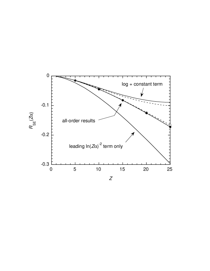
Figure 2: Comparisons between all-order and perturbative results of $R_{\text{SE}}(Z\alpha)$. Solid and dashed lines are $2p_{1/2}$ and $2p_{3/2}$ results, respectively. Closed and open circles are $2p_{1/2}$ and $2p_{3/2}$ all-order results, respectively.

Turning to the $2p$ E1 decay rates, we note that, while less severe than for M1 decays, there is still considerable cancellation present between the various contributions, particularly at low $Z$. This is of course required by the fact that the $Z\alpha$ expansion series for $R(Z\alpha)$ has no constant term, but instead starts in order $(Z\alpha)^{2}$. Again, the high degree of cancellation between contributing terms at low $Z$ serves as a check of our numerical calculations, but in this case, we can also compare our low-$Z$ results with the perturbation series. In Fig. 2, all-order results of $R_{\text{SE}}(Z\alpha)$ for $2p_{1/2}$ and $2p_{3/2}$ from Tables 3 and 4 are compared with analytic results from Eqs. (37) and (38). It can be seen that all-order results do converge to the analytic results at low $Z$. In particular, the leading logarithmic term in the perturbation series, which is the same for both $2p_{1/2}$ and $2p_{3/2}$, is good for $Z=1$ and 2 only, while including the constant terms, which leads to the splitting of fine structure results, extends the validity of the perturbation series to $Z=7$ or 8. This is typical of self-energy calculations where the $Z\alpha$ series is known to converge very slowly except at very low $Z$ and nonperturbative methods such as those shown here are needed for mid- to high-$Z$ ions.

In spite of the apparent agreement between the perturbation and all-order results shown in Fig. 2, it should be noted that there are residual, unresolved discrepancies between them. By extending the accuracy of our all-order calculations for $R_{\text{SE}}(Z\alpha)$ to a level of $\pm$0.0002 for low-$Z$ ions, we were able to extract values of 6.67 and 6.62 for the constant terms of the $2p_{1/2}$ and $2p_{3/2}$ states, respectively. While these results are uncertain to $\pm 0.20$ due to the high degree of numerical cancellation at low $Z$ when the leading logarithmic term is subtracted out, they are nevertheless different from the corresponding analytic values of 6.051 68 and 5.984 36 from Eqs. (37) and (38). Until this discrepancy is resolved, we would assign a 10% error to the constant terms, which should have negligible effect on $R_{\text{SE}}(Z\alpha)$ anyway.

While the decay rate corrections here are of intrinsic interest, the purpose of the present calculation is actually to serve as the first step in the calculation of PNC corrections. There is interest in the parity forbidden transition $6s_{1/2}\rightarrow 7s_{1/2}$ in cesium, which serves as one test of the electroweak part of the standard model of particle physics. A very large radiative correction has been found for this case Kuchiev , Milstein , but the only calculation using exact propagators that has so far been carried out was for the $2s_{1/2}-2p_{1/2}$ matrix element for hydrogenlike ions PNC . This calculation had the advantage of being gauge invariant because of the degeneracy of the Dirac energies of the two states. The calculation carried out in this paper is also gauge invariant despite the differing energies of the $n=2$ states and the ground state, and is generalizable to the PNC case. To carry out this generalization, the extra perturbation of the effect of $Z$ boson exchange between the nucleus and electron must be added.

An additional feature that must be dealt with for extending the present calculation to neutral cesium is the complication of dealing with a many-electron system. Because we use numerical Green’s functions, there is no difficulty in using a modified Furry representation of QED in which the Coulomb potential is replaced with a model potential that incorporates the dominant effect of electron screening. However, the effect of the filled xenon-like core will have to be taken into account, which will lead to extra diagrams. We are at present setting up calculations of radiative corrections to allowed transitions in the alkalis, in which these issues will arise, with the next step being the inclusion of the effect of $Z$ exchange.

The challenges to experiment in testing the calculations presented here are considerable. The largest radiative corrections found here are those to M1 decays at high $Z$, with the correction at $Z=100$ being 1.2%. For E1 decays, even the largest case, $2p_{1/2}$ at $Z=100$, has a radiative correction of only 0.2%. Rather than a direct measurement, experiments involving interference, such as the one discussed in Ref. Dunford , may be more promising.

There is a radiative correction, even though very small at low $Z$, that is of particular interest. It involves the E1 decay of the $2p_{1/2}$ state in hydrogen. One approach to the determination of the Lamb shift as described in Ref. Sok involves the measurement of the decay rate of the $2p_{1/2}$ state in hydrogen to very high accuracy. To interpret the experiment, Ref. Sok used the following formula for the radiative correction

$$R_{2p_{1/2}}(Z\alpha)\Big{|}_{\text{Ref.~{}\cite[cite]{\@@bibref{Authors Phrase1YearPhrase2}{Sok}{\@@citephrase{(}}{\@@citephrase{)}}}}}={32\over 3}\,(Z\alpha)^{2}\,\bigg{[}-\ln(Z\alpha)^{-2}-{1\over 8}\ln k_{0}(2P)+\ln k_{0}(1S)-{1\over 64}-{19\over 30}\,\bigg{]},$$ (71)

which can be shown to be equivalent to the first term of Eq. (17). However, as discussed in connection with the vacuum polarization contribution, using only the energy shift gives answers in significant disagreement with using both parts of Eq. (17). Our result, combining vacuum polarization with self-energy, is

$$R_{2p_{1/2}}(Z\alpha)\Big{|}_{\text{present work}}=(Z\alpha)^{2}\biggl{\{}\biggl{[}{8\over 3}\,\ln{4\over 3}-{61\over 18}\biggr{]}\!\ln(Z\alpha)^{-2}+6.576~{}03\biggr{\}}.$$ (72)

As noted earlier, we do have agreement with the logarithmic contribution found earlier by Ivanov and Karshenboim Ivanov . Using the hydrogenic value of $\Gamma_{0}$ (including recoil through a factor of $m_{r}/m_{e}$)

$$\Gamma_{0}(2p_{1/2})\Big{|}_{Z=1}=6.264~{}942~{}3\times 10^{8}~{}{\rm s}^{-1},$$

the radiatively corrected lifetimes of the $2p_{1/2}$ state for hydrogen are

$$\Gamma(2p_{1/2}) = 6.264~{}927~{}4\times 10^{8}~{}{\rm s}^{-1}~{}~{}\text{(present work)},$$

$$\Gamma(2p_{1/2}) = 6.264~{}922~{}3\times 10^{8}~{}{\rm s}^{-1}~{}~{}\text{(Ref.~{}\cite[cite]{\@@bibref{Authors Phrase1YearPhrase2}{Ivanov}{\@@citephrase{(}}{\@@citephrase{)}}})},$$

$$\Gamma(2p_{1/2}) = 6.264~{}881~{}2\times 10^{8}~{}{\rm s}^{-1}~{}~{}\text{(Ref.~{}\cite[cite]{\@@bibref{Authors Phrase1YearPhrase2}{Sok}{\@@citephrase{(}}{\@@citephrase{)}}})}.$$

As indicated earlier, Ref. Ivanov included only the logarithmic term, which was in agreement with our results, so the numerical difference shown above is due to the constant term in Eq. (72). The difference is under 1 part per million (ppm), which corresponds to under 1 kHz in the Lamb shift. However, there is a more significant 7 ppm difference with Ref. Sok , which should play a significant role in the interpretation of that experiment. Of course, this is only relevant if ppm precision can be reached experimentally. Issues involved in reaching this extremely high accuracy, which we note is two orders of magnitude greater than found in positronium orthoexp , have been discussed by Hinds Hinds .

Figure 1: Two-loop Lamb shift diagrams.

Table 1: Lowest-order one-photon decay rates to the ground state for $n=2$ states of hydrogenic ions in atomic units. Numbers in square brackets indicate powers of 10. The last column gives the nuclear fermi distribution parameter $c$ in fermis. Conversion to the unit of $s^{-1}$ is through 1 a.u. = $4.134~{}137\times 10^{16}~{}s^{-1}$.

$Z$	$2s_{1/2}$	$2p_{1/2}$	$2p_{3/2}$	$c$
5	5.9038[-16]	9.4779[-6]	9.4735[-6]	1.8104
10	6.0733[-13]	1.5172[-4]	1.5144[-4]	2.9889
15	3.5262[-11]	7.6868[-4]	7.6546[-4]	3.2752
20	6.3251[-10]	2.4321[-3]	2.4140[-3]	3.7188
25	5.9680[-9]	5.9461[-3]	5.8769[-3]	4.0706
30	3.7551[-8]	1.2351[-2]	1.2144[-2]	4.4454
40	6.9521[-7]	3.9207[-2]	3.8037[-2]	4.9115
50	6.8431[-6]	9.6268[-2]	8.8114[-2]	5.4595
60	4.5463[-5]	2.0100[-1]	1.8737[-1]	5.8270
70	2.3180[-4]	3.7535[-1]	3.4051[-1]	6.2771
80	9.8091[-4]	6.4597[-1]	5.6706[-1]	6.6069
90	3.6293[-3]	1.0440	8.8110[-1]	6.9264
100	1.2193[-2]	1.6033	1.2913	7.1717

Table 2: Breakdown of contributions to $R_{2s_{1/2}}(Z\alpha)$.

$Z$	$Q_{V1}$	$Q_{V2}$	$Q_{V3}$	$Q_{SL1}$	$Q_{SL2}$	$Q_{SR1}$	$Q_{SR2}$	$Q_{derb}$	$R(Z\alpha)$
50	-8418.269	-68461.495	78211.835	-10142.571	11.673	8593.159	11.810	192.382	-1.476
60	-2446.426	-14508.277	17540.361	-4213.698	11.696	3490.708	11.893	110.828	-2.915
70	-824.257	-4479.499	5587.689	-1990.665	11.725	1610.892	11.995	68.086	-4.034
80	-305.499	-1593.601	2044.727	-1034.946	11.762	817.408	12.121	43.683	-4.345
90	-119.499	-639.062	834.541	-580.832	11.808	446.644	12.277	28.790	-5.333
100	-47.230	-288.465	373.852	-347.601	11.867	259.536	12.474	19.246	-6.321

Table 3: Breakdown of contributions to $R_{2p_{1/2}}(Z\alpha)$.

$Z$	$Q_{V1}$	$Q_{V2}$	$Q_{V3}$	$Q_{SL1}$	$Q_{SL2}$	$Q_{SR1}$	$Q_{SR2}$	$Q_{derb}$	$R(Z\alpha)$
5	-9.551	-36.706	23.027	-0.013	11.626	-0.021	11.625	0.000	-0.014
10	-6.887	-28.062	11.756	-0.044	11.625	-0.064	11.630	0.000	-0.045
15	-5.403	-25.850	8.106	-0.082	11.627	-0.119	11.640	-0.001	-0.082
20	-4.409	-25.047	6.358	-0.126	11.631	-0.183	11.653	-0.003	-0.126
25	-3.685	-24.732	5.370	-0.173	11.635	-0.252	11.670	-0.003	-0.172
30	-3.131	-24.632	4.760	-0.222	11.641	-0.325	11.691	-0.012	-0.230
40	-2.344	-24.662	4.097	-0.319	11.655	-0.473	11.743	-0.031	-0.334
50	-1.822	-24.806	3.793	-0.409	11.673	-0.623	11.810	-0.065	-0.449
60	-1.464	-24.984	3.654	-0.488	11.697	-0.770	11.893	-0.121	-0.583
70	-1.219	-25.166	3.594	-0.553	11.727	-0.909	11.995	-0.207	-0.738
80	-1.057	-25.349	3.570	-0.599	11.764	-1.037	12.121	-0.334	-0.921
90	-0.962	-25.533	3.558	-0.629	11.812	-1.146	12.277	-0.521	-1.144
100	-0.928	-25.726	3.544	-0.637	11.876	-1.229	12.474	-0.800	-1.426

Table 4: Breakdown of contributions to $R_{2p_{3/2}}(Z\alpha)$.

$Z$	$Q_{V1}$	$Q_{V2}$	$Q_{V3}$	$Q_{SL1}$	$Q_{SL2}$	$Q_{SR1}$	$Q_{SR2}$	$Q_{derb}$	$R(Z\alpha)$
5	-9.551	-36.484	22.775	0.001	11.626	-0.006	11.625	0.000	-0.014
10	-6.888	-27.653	11.254	0.000	11.625	-0.014	11.630	0.000	-0.045
15	-5.406	-25.318	7.397	-0.001	11.627	-0.023	11.640	0.001	-0.082
20	-4.413	-24.381	5.418	-0.002	11.630	-0.033	11.653	0.004	-0.123
25	-3.690	-23.946	4.202	-0.004	11.635	-0.042	11.670	0.008	-0.166
30	-3.138	-23.732	3.368	-0.008	11.640	-0.050	11.691	0.014	-0.215
40	-2.352	-23.572	2.278	-0.022	11.656	-0.063	11.743	0.037	-0.295
50	-1.830	-23.555	1.579	-0.047	11.675	-0.075	11.810	0.082	-0.361
60	-1.470	-23.594	1.082	-0.087	11.698	-0.087	11.893	0.144	-0.421
70	-1.218	-23.661	0.710	-0.149	11.726	-0.102	11.995	0.242	-0.457
80	-1.043	-23.751	0.424	-0.237	11.758	-0.119	12.121	0.383	-0.464
90	-0.926	-23.863	0.204	-0.360	11.794	-0.140	12.277	0.585	-0.429
100	-0.856	-24.006	0.042	-0.527	11.833	-0.160	12.474	0.877	-0.323