PHOTON PHYSICS IN HEAVY ION COLLISIONS AT THE LHC

Abstract

Various pion and photon production mechanisms in high-energy nuclear collisions at RHIC and LHC are discussed. Comparison with RHIC data is done whenever possible. The prospect of using electromagnetic probes to characterize quark-gluon plasma formation is assessed.

1 INTRODUCTION

The production of photons in heavy ion collisions is rather complex and, in the standard approach, one roughly distinguishes three types of mechanisms:

$-\ 1)$ the photon is produced in the hard interaction of two partons in the incoming nuclei similarly to the well-known Chromodynamics (QCD) processes (QCD Compton, annihilation, bremsstrahlung) in nucleon-nucleon collisions. The rate is calculable in perturbative QCD and falls off at large transverse momentum, $p_{{}_{T}}$, as a power law. Photons are also produced as decay products of hadrons, such as of $\pi^{0},\eta,\cdots$, which are emitted in hard QCD processes and at large $p_{{}_{T}}$ the decay photon spectrum is also power behaved;

$-\ 2)$ in the collision of two nuclei the density of secondary partons is so high that the quarks and gluons rescatter and eventually thermalize to form a bubble of hot quark-gluon plasma: at LHC the initial temperature of the plasma is expected to be of the order of 1 GeV. It is assumed that the plasma evolves hydrodynamically. Photons are emitted in the collisions of quarks and gluons with an energy spectrum which is exponentially damped but which should extend up to several GeV;

$-\ 3)$ the QGP bubble expands and cools until a temperature of 150 to 200 MeV is reached and a hadronic phase appears. As they collide the hot hadronic resonances ($\pi^{0},\ \rho,\ \omega$) emit photons until the freeze-out temperature is reached. The typical energy of such photons ranges from several hundred MeV to several GeV.

In this standard picture it is expected that the thermal production mechanisms will produce an excess of photons with an energy of a few GeV. In the following we critically discuss each stage of the production processes. One of the main problems is the fact that the theoretical predictions suffer from very large uncertainties at each step of the above scenario.

The report is organized as follows:
chap. 2: nomenclature of photons according to their production mechanisms;
chap. 3: results of RHIC;
chap. 4: experimental aspects of photon detection at LHC;
chap. 5: inclusive photon and (background) $\pi^{0}$ production from perturbative QCD;
chap. 6: inclusive thermal photon and $\pi^{0}$ production;
chap. 7: comparison of thermal and non-thermal photon and $\pi^{0}$ production mechanisms;
chap. 8. preliminary studies on photon-jet and photon-particle correlations;
chap. 9: theoretical considerations on non equilibrium effects;
chap. 10: theoretical considerations on lattice calculations of dilepton rates.
Useful information on nuclear cross sections on the one hand, and on luminosities, acceptances, etc., on the other hand is collected in two appendices.

Chapters 3 and 4 contain the experimental part of the report. The PHENIX results on $\pi^{0}$ and $\gamma$ production are first reviewed before turning to a discussion of the experimental capabilities of ALICE, CMS and ATLAS for detecting pions and photons.

In Chaps. 5 to 8 quantitative studies of inclusive photon production are presented. Both “signal”, i.e. direct photons, and “background” i.e. photons from decay of resonances, are discussed. These studies are carried out using presently available tools and models and, whenever possible, uncertainties in the predictions are given. Proton-proton, proton-nucleus and nucleus-nucleus collisions are treated in parallel. Predictions are made for the ratio $\gamma_{\rm direct}/\gamma_{\rm all}$ or $\gamma_{\rm direct}/\pi^{0}$ which determine if the extraction of a direct photon signal is feasible. The production of low mass lepton pairs at large transverse momentum is presented as a channel complementary to real photon production: it is based on similar dynamics of production but suffers from different backgrounds.

Whenever possible we use two alternative models. On the one hand, the “standard” approach based on next-to-leading-order (NLO) QCD calculations to describe the hard processes together with a hydrodynamic model to describe the thermal evolution of the fireball produced in heavy ion collisions, and, on the other hand, the Dual Parton Model (DPM) which combines soft and hard leading-order (LO) dynamics and has been extremely successful in describing hadron-hadron scattering as well as fixed target nucleus-nucleus scattering. Surprisingly, predictions of the two models in nucleus-nucleus collisions turn out to be very similar despite the fact that the treatment of final state nuclear effects are quite different.

Exploratory studies on photon-jet, photon-hadron and photon-photon correlations are presented and the comparison between proton-proton and nucleus-nucleus scattering is made. Only the LO approximation is used and, for the latter two cases, only the signal is considered.

We conclude from these studies that:
– thermal photon production manifests itself by an enhancement in the inclusive photon spectrum at $p_{{}_{T}}$ values below 10 to 15 GeV/c at the LHC. The shape of the transverse momentum spectrum may also be indicative of the production mechanisms;
– the $\gamma_{\rm direct}/\pi^{0}$ ratio in nucleus-nucleus collisions should be large enough to allow for the extraction of a direct photon signal, however the uncertainties on the predictions are large mainly due to the poor knowledge of the model parameters;
– the lepton pair channel at large momentum transfer looks promising but further detailed studies are necessary to determine if the large background from uncorrelated pairs can be reliably subtracted;
– correlation studies show characteristic changes of shapes in A+A collisions compared to $pp$ collisions but, here again, further studies are necessary concerning the background.

Many of the results presented are new, in particular, the comparison between two alternative models as well as the extensive discussion on the uncertainties at the LHC (role of the initial conditions of thermalization, chemical equilibrium vs. non equilibrium, $\cdots$), the studies of the lepton pair spectrum as well as that of the correlations involving a photon.

Chapters 9 and 10 are of a different nature and address more fundamental issues. Some of the basic hypotheses upon which the thermal production studies are based are critically analysed.

In Chap. 9, the relevance of the finite life-time of the thermal system is adressed and it is shown that recent claims of a very large production rate of photons due to this finite life-time are not tenable since they are based on a defective modeling of the system. This is an original piece of work. Furthermore, ways to deal with this problem in a realistic way are sketched.

In Chap.10, the improved perturbative methods upon which the calculation of thermal photon rates are based are compared with the non-perturbative lattice based method in a simple example, namely the production of a static lepton pair. The two approaches seem to indicate a large discrepancy both in the magnitude of the rate as well as in the functional dependence on the lepton pair mass. The error bars in both predictions are very large however and it is premature to conclude if a real contradiction between the two results exists. This is a very interesting problem and, clearly, further studies are called for.

This report is far from being the definitive work on photon, dilepton and pion production in heavy ion collisions at the LHC. The results are sufficiently interesting however to motivate more detailed theoretical and phenomenological studies on these topics.

2 PHOTONS AND PHOTONS

We define the “inclusive” photon spectrum in the usual sense: it is the unbiased photon spectrum observed in a collision between two hadrons or a hadron and a nucleus or two nuclei. This spectrum is built-up from a “cocktail” of many components:

– “prompt” photons which are produced, early in the collision, in hard QCD processes. They are directly emerging from a hard process or produced by bremsstrahlung in a hard QCD process. The associated spectrum is power behaved and dominates at large transverse momentum;

– “thermal” photons which are emitted in the collisions of quarks and gluons in the QGP phase or in scattering of hadronic resonances in hot matter; their spectrum is exponentially damped at large enough energy;

– “decay” photons are decay products of hadronic resonances (essentially $\pi^{0}$ and $\eta$). These resonances can be either produced in hard QCD processes (and the corresponding decay photon spectrum will be power behaved) or at the end of the thermal evolution of the system;

– “direct” photons are the sum of “prompt” and “thermal” photons. They can be obtained experimentally by subtracting from the inclusive spectrum the contribution from the “decay” photons which constitute a reducible background.

In heavy ion collisions, the aim is the extraction of the “thermal” signal: it can only be done by subtracting from the “direct” photon spectrum the contribution of the “prompt” photons (which are an irreducible background to direct thermal photons) calculated from theory. Therefore it is of utmost interest to correctly estimate the latter component. A prerequisite is a precise control of the photon production rate in proton-proton and proton-nucleus collisions.

One also defines in the context of thermal production “soft” and “hard” photons. The “soft” photons have an energy much less that the temperature of the medium while the “hard” ones have an energy of the order of the temperature or larger. This terminology is somewhat different from that used in the context of perturbative QCD. Only hard thermal photons are of interest for phenomenological studied since soft ones are overwhelmed by the background.

3 NEUTRAL PION AND PHOTON RESULTS FROM RHIC

G. David

The first three years of RHIC experiments brought spectacular results at an impressive pace. After producing the first Au+Au collisions at $\sqrt{s}=130$ GeV June 12, 2000, the accelerator delivered significant integrated luminosity (Table 1) and by QM’01 (January 2001) many exciting analyses were completed and presented. Maybe the most intriguing observation reported was the large suppression of high $p_{{}_{T}}$ neutral pions and charged hadrons in central collisions with respect to peripheral or $pp$ collisions [1] scaled with the number of nucleon-nucleon collisions. In Run-2 RHIC operated at $\sqrt{s}=200$ GeV producing both Au+Au [2, 3] and polarized $pp$ collisions [4]. The suppression of high $p_{{}_{T}}$ hadrons in central Au+Au collisions has been confirmed and the measurement extended to $\sim$ 10 GeV/c, while the $pp$ data provided neutral pion spectra up to 13 GeV/c. Therefore, the nuclear modification factor could be established with $\pi^{0}$ measured in the same experiment. However, it remained an open issue whether the suppression is an initial state or final state effect. Proving its versatility in Run-3 RHIC delivered D+Au collisions [5, 6] (and once again polarized $pp$) which were analyzed extremely fast and the results were published less than three months after data taking. These results essentially ruled out initial state effects as cause of the high $p_{{}_{T}}$ suppression observed in Au+Au collisions at RHIC energies.

Meanwhile, few and only preliminary results on inclusive and direct photon production became public. This is understandable since the photon measurement is much more difficult than the (correlation-type) $\pi^{0}$ measurement, and also because claiming any excess photons over the abundant background from hadron decays assumes that spectra of the contributing hadrons themselves ($\pi^{0},\eta,...$etc.) are known to high precision. First published photon results from RHIC are expected by the end of 2003, initially addressing the high $p_{{}_{T}}$ region where photon identification is least problematic.

One of the strengths of the RHIC program is a certain redundance within and overlap between experiments. In particular, photon and $\pi^{0}$ measurements - while mostly done in PHENIX with the electromagnetic calorimeters [7] - are also possible both in STAR and PHENIX via photon conversion which serves not only as a cross-check but helps to extend the spectra to very low $p_{{}_{T}}$. In addition, even within PHENIX there are two different electromagnetic calorimeters using different technologies and analyzed separately. The fact that one can make independent measurements of the same observable within the same experiment greatly increases the confidence in the ultimate results.

Run/date	Species	$\sqrt{s}$	Int. luminosity	Submitted publications
Run-1
June-Sep 2000	Au+Au	130 GeV	1$\mu$b-1	PRL 88, 022301 (2002)
Run-2
Sep-Nov 2001	Au+Au	200 GeV	24$\mu$b-1	PRL 91, 072301 (2003)
				NPA 715 (2003) 683c
				NPA 715 (2003) 691c
Dec 2001 - Jan 2002	$pp$	200 GeV	0.15pb-1	hep-ex/0304038 v2 ($\rightarrow$PRL)
Run-3
Nov 2002 - Mar 2003	D+Au	200 GeV	2.7nb-1	PRL 91 072303 (2003)
Apr 2003 - Jun 2003	$pp$	200 GeV	0.35pb-1

Table 1: Overview of RHIC runs as of June 2003. Integrated luminosity is given for PHENIX (which is typically the highest for the four RHIC experiments). In the last column we only list the final (submitted) publications on $\pi^{0}$ and published QM’02 preliminary results on photons.

3.1 $\pi^{0}$ spectra at RHIC

One of the first and still most intriguing results from RHIC was the observation in Run-1 ($\sqrt{s}=130$ GeV) that in central Au+Au collisions the yield of high $p_{{}_{T}}$ $\pi^{0}$-s was strongly suppressed with respect to expectations from $pp$ results at comparable energy scaled by the calculated number of binary nucleon-nucleon collisions (Fig. 2), although the same collision scaling described the peripheral data adequately [1]. Despite the large errors the effect was significant ($>2.5\sigma$), but low integrated luminosity and an only partially instrumented calorimeter prevented PHENIX from exploring it past $p_{{}_{T}}=4$ GeV/c. In Run-2 the combination of higher c.m. energy ($\sqrt{s}=200$ GeV), much higher statistics, and a fully instrumented detector made it possible to extend the minimum bias $\pi^{0}$ $p_{{}_{T}}$ spectra up to 12 GeV/c, and the semi-inclusive spectra up to 6-10 GeV/c, depending on the centrality class (Fig. 2).

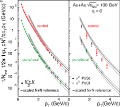
Figure 1: PHENIX results from 130 GeV Au+Au collisions (Run-1). The yields per event at mid-rapidity for (left) charged hadrons and (right) neutral pions are shown as a function of $p_{{}_{T}}$ for 60–80% (lower) and 0–10% (upper) event samples, with the $\pi^{0}$ results from the PbSc and PbGl analyses plotted separately. The error bars indicate the statistical errors on the yield; the surrounding brackets indicate the systematic errors. Shown for reference are the yields per collision in N+N collisions, of charged hadrons and neutral pions respectively, each scaled up by $\langle N_{coll}\rangle$ for the class. The bands indicate both the uncertainty in the N+N reference and in the determination of $\langle N_{coll}\rangle$.

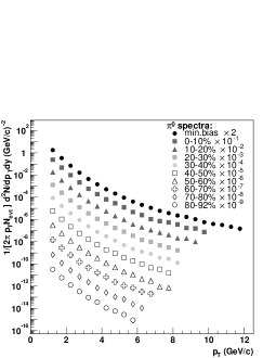
Figure 2: PHENIX results from 200 GeV Au+Au collisions (Run-2). Invariant yields of $\pi^{0}$ at mid-rapidity are plotted as a function of $p_{{}_{T}}$ for minimum bias and 9 different centrality selections (0-10% is the most central, 80-92% is the most peripheral). The yields are scaled for clarity.

The deviation from simple scaling with the number of nucleon-nucleon collisions $N_{coll}$ (or, more rigorously, with the nuclear overlap function $T_{AB}$) is usually characterized by the nuclear modification factor $R_{AA}$ defined as

$$R_{AA}(p_{{}_{T}})\,=\,\frac{(1/N^{evt}_{AA})\,d^{2}N^{\pi^{0}}_{AA}/dp_{{}_{T}}dy}{\langle N_{coll}\rangle/\sigma_{pp}^{inel}\,\times\,d^{2}\sigma^{\pi^{0}}_{pp}/dp_{{}_{T}}dy},$$ (1)

the expectation being that starting at some relatively low $p_{{}_{T}}$ (1.5-2.0 GeV/c) which marks the approximate transition from “soft” to “hard” physics and where jets become dominant $R_{AA}$ reaches unity because higher $p_{{}_{T}}$ particles are produced in incoherent, large momentum transfer parton-parton scatterings whose (small) probability in turn is proportional to the number of nucleon-nucleon collisions $N_{coll}$. At lower $\sqrt{s}$ (SPS-energies) $R_{AA}$ even rises above unity (Cronin-effect) due to multiple scattering of partons before the large $Q^{2}$ process initiates the jet. In stark contrast to that expectation of $N_{coll}$ scaling or some enhancement $R_{AA}>1$, PHENIX found already at $\sqrt{s}=130$ GeV (Run-1) that for $\pi^{0}$ in central Au+Au collisions $R_{AA}$ never reaches unity. Instead, after reaching its maximum at $p_{{}_{T}}\simeq 1.5$ GeV/c it decreases for higher transverse momenta (Fig. 3) to about 0.3. In other words, there is a factor of $\sim$3 suppression already around $p_{{}_{T}}=3$ GeV/c. On the left panel of Fig. 3 $R_{AA}$ is plotted for $\pi^{0}$ and charged hadrons ($(h^{+}+h^{-})/2$ in the most central Au+Au collisions with $N_{coll}$ calculated from the Glauber-model. The suppression at higher $p_{{}_{T}}$ is even more dramatic when compared to the enhancement observed in Pb+Pb at $\sqrt{s}=17.3$ GeV and $\alpha+\alpha$ at $\sqrt{s}=31$ GeV, also shown on the plot. On the right panel of Fig. 3 the ratio of central to peripheral data - both normalized with $N_{coll}$ - is shown. The behavior is very similar to $R_{AA}$, but the $p_{{}_{T}}$ coverage is somewhat less since the peripheral spectrum has a smaller range. It should be pointed out that $R_{AA}$ and the central/peripheral ratio (often referred to as $R_{CP}$) are dominated by different systematic errors, so the combined “message” of the two results (significant suppression) is even stronger than suggested by the error-bars on any one of them. Also, uncertainty on $\sigma_{pp}^{inel}$ cancels to first order in the central to peripheral ratio (right panel).

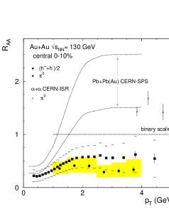
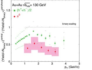
Figure 3: PHENIX results from 130 GeV Au+Au collisions (Run-1). Left panel: the ratio $R_{AA}$ for charged hadrons ($(h^{+}+h^{-})/2$) and neutral pions in central Au+Au collisions. The error bars indicate the statistical errors, the surrounding bands (shaded for $\pi^{0}$’s, brackets for $(h^{+}+h^{-})/2$) indicate the combined statistical and systematic errors on the ratio, including the uncertainty in the $pp$ data and the uncertainty in $\langle N_{coll}\rangle$. Also shown for reference are $R_{AA}$ for $\alpha+\alpha$ ($\sqrt{s}=31$ GeV) and for central Pb+Pb collisions ($\sqrt{s}=17.3$ GeV) measured at the CERN-SPS. Right panel: Ratio of central to peripheral $p_{{}_{T}}$ spectra (both normalized with the calculated $N_{coll}$) for charged hadrons and $\pi^{0}$.

The observed suppression was a very strong indication that an extremely hot and dense medium has been created in central Au+Au collisions which by some mechanism depleted the number of high $p_{{}_{T}}$ jets. However, it was unclear whether the very creation of the jets was suppressed (e.g. due to initial state parton saturation) or the jet production itself was the same as in $pp$, scaled by $N_{coll}$, but the jets lost a significant fraction of their energy while traversing the medium (as predicted by different models of jet quenching). Also, in case of energy loss the nature of the medium causing the loss (partonic or hadronic) was unclear. Finally, various theoretical scenarios predicted similar suppression at 3-4 GeV/c (the upper limit of the Run-1 results), but predicted different $p_{{}_{T}}$ dependence of the suppression at transverse momenta beyond that range.

In Run-2 RHIC delivered Au+Au and $pp$ collisions at $\sqrt{s}=200$ GeV, both at sufficiently high integrated luminosity such that the $\pi^{0}$ $p_{{}_{T}}$ spectra could be extended to 10-13 GeV/c. The $pp$ results are described elsewhere in this Report and in [4], but it should be emphasized once again that measuring the reference $pp$ spectrum in the very same experiment (i.e. with similar systematics) greatly reduces the systematic error on $R_{AA}$ proper. The nuclear modification factor using $\pi^{0}$-s in the most peripheral and most central Au+Au collisions is shown on Fig. 5, where this time $R_{AA}$ was calculated using the PHENIX $pp$ measurement. Perfect scaling with $N_{coll}$ would mean $R_{AA}=1$. Although averaging below one, the peripheral data are certainly consistent with $N_{coll}$ scaling within errors. However, in central collisions the suppression is unambiguous in the entire $p_{{}_{T}}$ range. $R_{AA}$ reaches its highest value (smallest suppression, $\sim$2.5) around 2 GeV/c, then decreases, and is constant within errors above 4 GeV/c, giving a suppression factor of 4-5. While this result disfavored those quenching models that predict a $p_{{}_{T}}$ dependence of the suppression, it did not differentiate between initial state and final state effects, nor could it distinguish between partonic and hadronic energy loss scenarios.

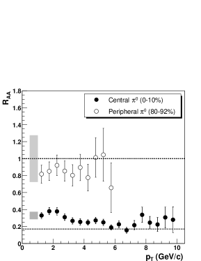
Figure 4: PHENIX results from $\sqrt{s}$ = 200 GeV. Nuclear modification factor $R_{AA}(p_{{}_{T}})$ for $\pi^{0}$ in central (closed circles) and peripheral (open circles) Au+Au collisions. The error bars include all point-to-point experimental ($pp$, Au+Au) errors. The shaded bands represent the fractional uncertainties in $\langle T_{AuAu}\rangle$ and in the $\pi^{0}$ yields normalization added in quadrature, which can move all the points up or down together (in the central case the shaded band shown is the fractional error for the first point).

Figure 5: Top: Nuclear modification factor $R_{\rm{dA}}$ for $(h^{+}+h^{-})/2$ in minimum bias D+Au compared to $R_{\rm{AA}}$ in the 10% most central Au+Au collisions. Inner bands show systematic errors which can vary with $p_{{}_{T}}$, and outer bands include also the normalization uncertainty. Bottom: Comparison of $R_{\rm{DA}}$ for $(h^{+}+h^{-})/2$ and the average of the $\pi^{0}$ measurements in D+Au. The bar at the left indicates the systematic uncertainty in common for the charged and $\pi^{0}$ measurements.

Therefore, the major part of Run-3 at RHIC has been dedicated to D+Au collisions at $\sqrt{s}=200$ GeV, under the assumption that in D+Au collisions the gold nucleus remains “cold”, and any effects due to a hot, dense medium in the final state would be absent. On the other hand if an initial state effect in the Au nucleus is responsible for the observed suppression, such suppression should manifest itself in D+Au collisions, too. Note, that the choice of deuterium (D+Au) instead of proton ($p$Au) was motivated by purely technical reasons, and it has been demonstrated that there is little if any difference in the physics of +DAu and $p$Au collisions at these energies [5] – an interesting observation in its own right. The nuclear modification factor for D+Au is shown on Fig. 5 for charged particles and neutral pions. The suppression observed in central Au+Au collisions is clearly absent here. This result indicates that the suppression in central Au+Au collisions is not an initial state effect, nor does it arise from modification of parton distribution functions in nuclei. Further analyses including a detailed study of the centrality dependence of $R_{dA}$ may shed further light on the mechanism of suppression.

There is a substantial effort in PHENIX to extract the $\eta$ yield from Run-2 Au+Au data and to establish the asymptotic $\eta/\pi^{0}$ ratio, but no results have been presented yet. STAR published $K^{0}_{S}$ spectra at $\sqrt{s}=130$ GeV using the $K^{0}_{S}\rightarrow\pi^{+}\pi^{-}$ channel [8], but only at $p_{{}_{T}}<1.5$ GeV/c. Both $\eta$ and $K^{0}_{S}$ have $\pi^{0}$ decay channels and thus “feed down” into the $\pi^{0}$ spectrum but due to the (two- and three-body) decay kinematics this contamination (as well as contributions from higher mass mesons) is negligible if compared to current experimental errors [2].

Using the published $\pi^{0}$ data at 130 GeV and the preliminary 200 GeV $\pi^{0}$ data a first study of $x_{T}$ scaling has been presented at the Fall 2002 DNP meeting [9]. At both energies suppression of high $p_{{}_{T}}$ $\pi^{0}$ with respect to point-like scaling from $pp$ collisions has been observed. If the effect is due to shadowing of the structure functions rather than a final state interaction with the hot medium, the yields at a given $x_{T}$ and centrality should exhibit the same suppression and the scaling exponent $n(x_{T},\sqrt{s})$ should remain unchanged from $pp$ to Au+Au collisions. The study found that, within systematic errors, $x_{T}$ scaling with $n(x_{T},\sqrt{s})=6.3\pm 0.6$ applies for both peripheral and central collisions in the range $0.025\leq x_{T}\leq 0.06$.

3.2 Inclusive and direct (non-hadronic) photons

While $\pi^{0}$ spectra have already been published from all three RHIC runs, so far only preliminary results were shown on photons. Though counterintuitive at first, measuring photons - even the inclusive photon spectrum - is much more difficult than measuring $\pi^{0}$-s. Neutral pions are usually reconstructed from a correlation and - except for very high $p_{{}_{T}}$ and/or very low multiplicities - they are measured only statistically, calculating invariant mass from all photon candidates in an event rather than trying to identify both decay photons from a particular $\pi^{0}$. Moreover, at low multiplicities ($pp$, D+Au, peripheral Au+Au) an accurate $\pi^{0}$ spectrum can be extracted without any photon identification at all – just by calculating the invariant mass from pairs of all clusters in an event. Even in high multiplicity events good photon identification and effective rejection of other particles is not crucial. Also, since the true mass of $\pi^{0}$ is known, the measurement is “self-calibrating” in the sense that any shift in the observed centroid and any widening of the mass peak corresponds to a calculable shift in the (apparent) transverse momentum and can be corrected for. Finally, many of the pions created outside the collision vertex do not reconstruct with the proper invariant mass due to the mismatch between the true and the apparent opening angle of the two photons. Therefore, many of those “background” $\pi^{0}$-s don’t contribute to the raw yields, and don’t have to be corrected for.

The situation with the inclusive photon spectrum is entirely different. Obviously particle identification and a very precise knowledge of its efficiency is essential. Usually there is no straightforward way to check the energy (and $p_{{}_{T}}$) scale, although - depending on the slope - just 1% error on the energy can give up to 10% error on the cross-section. Unless the direction of the photon is measured, there is little if any rejection/identification of photons not coming from the collision vertex.

While inclusive photon spectra ($\gamma_{\rm inc}$) are important in their own right, the exciting new physics is hidden in the “direct” or “excess” photon spectrum ($\gamma_{\rm dir}$), the difference of inclusive photons and photons from electromagnetic decays of final state hadrons ($\gamma_{\rm decay}$). Since $\gamma_{\rm decay}$ is simulated using fits to the measured $\pi^{0},\eta,...$ spectra, reliable hadron spectra are a prerequisite to the direct photon measurement and many (although not all) of the errors on hadron spectra will propagate into the direct photon spectrum.

Finally, a good direct photon measurement will have to reveal not only the magnitude of photon excess over hadronic sources $\gamma_{\rm inc}-\gamma_{\rm decay}$ but also make the decomposition of at least three overlapping spectra possible (hard scattering, plasma phase, final state radiation). Therefore, the errors both on shape and absolute normalization should be very small. Once this ambitious goal is reached, one can work backwards (starting with the highest available $p_{{}_{T}}$) in unfolding the contributions of the different photon production processes. Once a high quality $\gamma_{\rm dir}=\gamma_{\rm inc}-\gamma_{\rm decay}$ “direct” (excess) photon spectrum is available, starting at the highest transverse momenta one can try to fix the pQCD scale and improve upon fragmentation functions in $pp$ as well as establish the effects of the medium in Au+Au. Next, this pQCD contribution has to be subtracted from $\gamma_{\rm dir}$. The result at a few GeV/c is expected to be dominated by radiation from the early plasma. (Cross-checks with D+Au collisions will decrease the uncertainties). Then once again one can go lower in $p_{{}_{T}}$ (i.e. later in evolution time) to look for radiation from the plasma - hadronic gas phase transition, and so on. Whereas the spectral shapes of different contributors are different, deconvolution of these spectra obviously requires unprecedented accuracy on the $\gamma_{\rm dir}$ excess photon spectrum (which implies a comparable accuracy of the $\pi^{0}$ spectra themselves).

Preliminary results from PHENIX at $\sqrt{s}=130$ GeV (presented at QM’02) are shown on Fig. 6 for peripheral collisions (left panel) and central collisions (right panel). The plots show the ratio $\gamma_{\rm inc}/\gamma_{\rm decay}$ of the inclusive photon spectrum and the photon spectrum expected from final state hadron decays. A fit to the measured $\pi^{0}$ spectrum is used to calculate $\gamma_{\rm decay}$ with a fast Monte-Carlo program; $m_{{}_{T}}$ scaling is assumed for $\eta$ (higher mass mesons are not included). The band indicates the systematic errors, completely dominated by the uncertainties of the fit itself. Note that in Run-1 the $\pi^{0}$ measurement extended only until $p_{{}_{T}}=4$ GeV/c with large errors (Fig. 2). Therefore, the fit was not very well constrained, both the absolute normalization and the shape can vary significantly. Photon identification is based solely on shower shape and timing - charged particle veto is not applied. Fluctuations of the points indicate that the $1\sigma$ errors are not overestimated. Within errors the results are consistent with no photon excess over known hadronic sources, but obviously the sensitivity of the measurement is low.

Preliminary results from PHENIX at $\sqrt{s}=200$ GeV (presented at QM’02) are shown on Fig. 7 for peripheral collisions (left panel) and central collisions (right panel). Different from the 130 GeV data, here the double ratio $(\gamma_{meas}/\pi^{0}_{meas})/(\gamma_{sim}/\pi^{0}_{sim})$ is plotted, where the subscript _meas refers to the measured inclusive photon and $\pi^{0}$ spectra, $\pi^{0}_{sim}$ is a fit to the measured $\pi^{0}$ spectrum which is then used in a Monte-Carlo to generate the photon spectrum $\gamma_{sim}$ expected from hadronic decays. In the absence of any non-hadronic sources this double ratio would be exactly one, which is clearly the case in peripheral collisions (left panel). One should appreciate the large, non-statistical fluctuations of the points even at low $p_{{}_{T}}$ - indicating that the errors are once again not overestimated. Data do not extend as far in $p_{{}_{T}}$ as for $\pi^{0}$-s, to avoid large uncertainties of the $\pi^{0}$ fit in the tail and beyond the measured range. The double ratio for central events (right panel) is still consistent with no excess within errors, but obviously exhibits a suggestive trend.

The STAR collaboration also presented preliminary results on excess photons at QM’02 [11]. In this measurement photons converted to $e^{+}e^{-}$ pairs in the silicon vertex tracker and the inner field cage of the TPC were analyzed. The experiment found that above $p_{{}_{T}}=1.65$ GeV/c the contribution from $\pi^{0}$ to the inclusive photon spectrum decreases in the most central events (0-11% centrality), indicating an increase in contribution from other photon sources, possibly other electromagnetic decays or direct photons. However, there is a significant uncertainty in the normalization of the $\pi^{0}$ spectra.

3.3 Outlook

Obviously, the carefully worded statements from both experiments reflect the technical difficulties and do not exclude a possibly substantial yield of direct photons. Results with reduced systematic errors can be expected within a year and at larger $p_{{}_{T}}$ will provide the first tests of pQCD calculations. However, as emphasized in other sections of this Report, measuring the photon excess over the yield expected from hadron decays is only the first step: much of the interesting physics lies is hidden in the composition of this excess. In order to disentangle the contributions from hard scattering, the QGP, the mixed and the hadronic phases one has to measure this excess both in a very wide $p_{{}_{T}}$ range and with unprecedented accuracy. This is and continues to be the biggest challenge to the experimentalists.

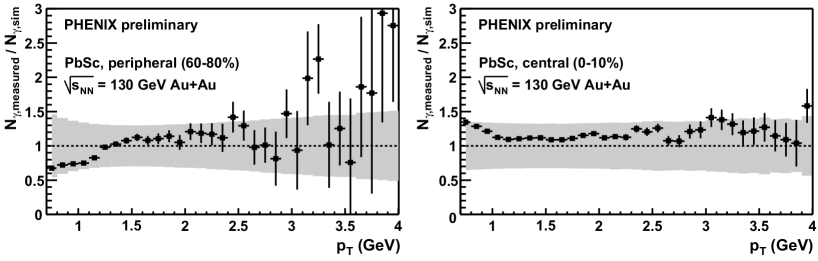
Figure 6: Ratio of inclusive photon spectrum to the photon spectrum expected from hadron decays in $\sqrt{s}=130$ GeV Au+Au collisions, in peripheral events (left panel) and central events (right panel). The shaded bands are the systematic errors dominated by the uncertainties of the (measured) $\pi^{0}$ spectrum

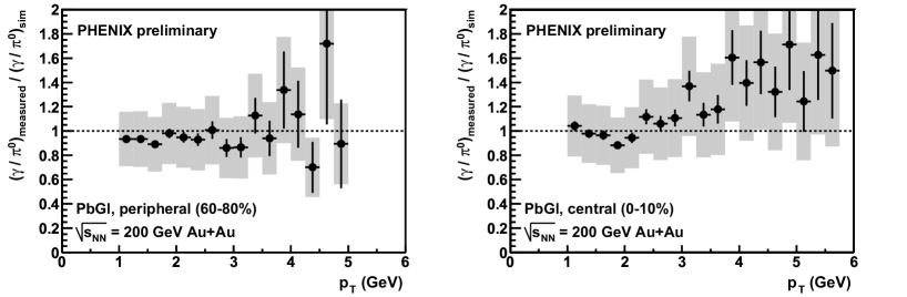
Figure 7: Measured over expected $\gamma/\pi^{0}$ ratio in Au+Au collisions at $\sqrt{s}$=200 GeV in peripheral (left panel) and central (right panel) collisions. “Expected” means that all photons are assumed to come from hadron decays, and the double ratio eliminates certain systematic errors. A ratio of unity means that all photons come from hadron decays. The shaded boxes represent the estimated $1\sigma$ systematic errors on the data points.

Therefore, it is instructive to briefly review the dominant sources of systematic errors on $\gamma_{\rm inc}/\gamma_{\rm decay}$ in the current analyses. At RHIC the errors on $\pi^{0}$ are currently around 14-17%, distributed about equally between yield extraction, particle identification and effects of the energy scale, and this determines the accuracy of the calculated $\gamma_{\rm decay}$. Contributions from other mesons are currently not measured (although analyses of $\eta$ as well as $K^{0}_{S}$ above 1.5 GeV/c by charged pions are under way).

For the inclusive photon analysis photon efficiency has about the same error as in the $\pi^{0}$ measurement, but hadron contamination is added. The energy scale uncertainties have bigger weight (because of the lack of “self-calibration”, the possibility to cross-check the energy scale using the invariant mass), and a major contributor to the errors is the instrumental background. Note that three of these contributors (particle identification, contamination and background) become worse as one tries to move to lower transverse momenta (thermal region).

On the other hand it is exactly at low $p_{{}_{T}}$ where the complementary measurements via conversion electrons in both PHENIX and STAR offer advantages: since they provide directional information, much of the instrumental background, and, in general, photons not from the vertex can be eliminated. Some upgrades of current RHIC detectors point in this direction, too. Also, new types of analyses are developed to reduce systematic errors. While trying to defeat all sources of systematic errors is probably a futile excercise one can make independent measurements of the same quantity, within the same experiment, with very different systematics, thus increasing the level of confidence in the results. Photon measurements are notoriously difficult: the author thinks future LHC experiments are well advised to include such “redundancies” from the very beginning.

4 DETECTOR STUDIES, RESOLUTION

In this section one briefly describes the main features of ALICE, CMS and ATLAS concerning photon and hadron detection. The acceptances for each detector are summarized in appendix 2.

4.1 Photon detection at ALICE

H. Delagrange, D. d’Enterria, T. Peitzmann, Yu. Kharlov

The ALICE detector [12] aims to study the physics of strongly interacting matter at extreme energy densities, where the formation of a new phase of matter, the quark-gluon plasma, is expected. Among all the probes of the quark matter, photons could be used to study the dynamics of strong interactions in hadronic collisions. Owing to their small electromagnetic coupling, produced photons do not interact with the surrounding matter and thus probe the properties of the matter at the time of their production [13].

4.1.1 Photon spectrometer PHOS in ALICE

In ALICE, the photon spectrometer PHOS is designed [14] to detect, identify and measure with high resolution the 4-momenta of photons. Photon studies in heavy ion collisions require from the detector a high discrimination power between photons and any other kind of particles, charged and neutral hadrons or electrons. The best possible resolutions in energy and position, as well as a reasonably large acceptance provide a high neutral meson identification and, thus, the high precision determination of the background for the direct photon spectrum.

The final design of the photon spectrometer PHOS consists of five identical modules positioned at the bottom of the ALICE detector (Fig.8).

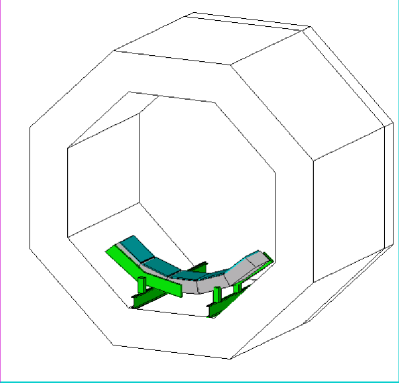
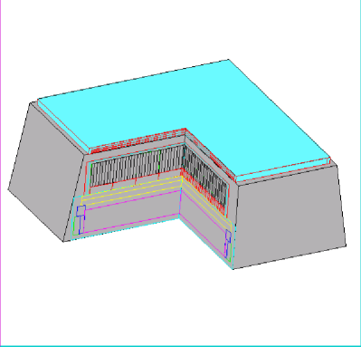
Figure 8: The PHOS detector: PHOS inside the ALICE solenoid magnet (left), and one PHOS module (right).

The PHOS modules are positioned at the distance 4.6 m from the beam interaction point and installed at the azimuth angles $\pm 40.7^{\circ},\pm 20.3^{\circ}$, and $0^{\circ}$. Each module consists of the electromagnetic calorimeter detector (EMC) and a charged particle veto detector (CPV).

Each EMC module is constructed as a matrix of $64\times 56$ cells of lead tungstate (PbWO₄) scintillator crystals. Each crystal, elementary unit of the calorimeter, is an 18 cm long parallelepiped providing 20 units of radiation length (X${}_{\rm 0}=0.89$ cm). It is shaped with a squared cross-section of 22$\times$22 mm², to be compared to the Molière radius of lead tungstanate, $r_{M}=20$ mm. The scintillation light, in the visible near UV-wavelength range, is read out by a 5$\times$5 mm² avalanche photo-diode (APD) integrated with a low-noise pre-amplifier. The calorimeter is operated at low temperature, $-25~{}^{\circ}$C, stabilized to $\pm 0.3^{\circ}$ C. This operation mode on one hand enhances the scintillation light output by a three fold factor and provides the required high and constant energy resolution even for the less energetic photons and, on the other hand, keeps the noise of the APD low enough to provide a high signal to noise ratio. The electronic chain associated to each crystal of the PHOS spectrometer delivers two energy signals, one with low- and one with high gain, proportional to the energy deposited in the crystal and a timing signal that measures the time of the particle impact with respect to a trigger time reference.

The CPV consists of multiwire proportional chambers with cathode pad read-out. Each calorimeter module is covered by a CPV module with an active area of 144.6$\times$144.6 cm², 1.3 cm deep and filled with a gas mixture 70% Ar and 30% CO₂. The total thickness of the CPV module is 5.1 cm. Low-mass construction materials are used for the CPV construction to minimize the material budget, radiation length and detector mass. The anode wires of the proportional chamber are strung along the beam direction with a wire pitch of 5.65 mm and placed at 5 mm above the cathode. The cathode is segmented in 64 (along beam direction)$\times$128 (across beam direction) rectangular pads of 2.26$\times$1.13 cm², elongated along the anode wires. The electron shower induced by the passage of a charged particle is collected on the cathode and an induced charge is retrieved from each pad of the CPV.

The PHOS acceptance in pseudorapidity is defined by $|\eta|<0.13$. Each of five modules covers $17.8^{\circ}$ in azimuth angle.

4.1.2 Intrinsic performance of PHOS

The two parameters that describe the response of the EMC spectrometer and play the most important role for photon identification are the resolutions in energy and position. The energy resolution depends on the spectrometer ability to collect most of the electromagnetic shower energy, convert it into visible light and transmit it to the APD, as well as on the APD photo-efficiency and photon electron gain factor. The position resolution depends on the segmentation of the spectrometer and energy resolution.

To determine experimentally these features an electron beam of energy ranging from 0.6 to 4.5 GeV irradiated the central module of an array of $3\times 3$ EMC modules. A Gaussian function was adjusted to the distribution of total energy, E, collected in the array. The resulting resolution, $\sigma/E$, was compared (Fig. 9)

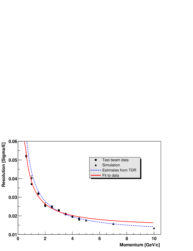
Figure 9: Energy resolution of a $3\times 3$ EMC array measured in response to mono energetic electrons ($\bullet$) or calculated with simulations of mono energetic photons ($\blacktriangle$). The continuous line represents the result of the fit of Eq. (2) to the data and extrapolated to 10 GeV. The dashed line represents the values quoted in the TDR [14].

to the one obtained by the simulation performed in exactly the same conditions as the experiment. The following parametrization was adjusted to the experimental resolution dependence on electron energy:

$$\frac{\sigma}{E}=\sqrt{\frac{a^{2}}{E^{2}}+\frac{b^{2}}{E}+c^{2}}$$ (2)

where E is in units of GeV, a represents the contribution of the electronic noise, b the stochastic term, and c the constant term.

The impact position on PHOS is reconstructed by calculating the position of the center of gravity of the reconstructed cluster. This position is further corrected for the incidence direction of the impinging photon. The previously discussed test beam measurements were extended to verify the influence of the photon incidence on the position resolution by tilting the array of EMC modules by 0, 3, 6 and 9^∘. Fig. 10 shows the r.m.s. of the Gaussian fit of this distribution versus the photon energies from 1 to 50 GeV for several incidence angles.

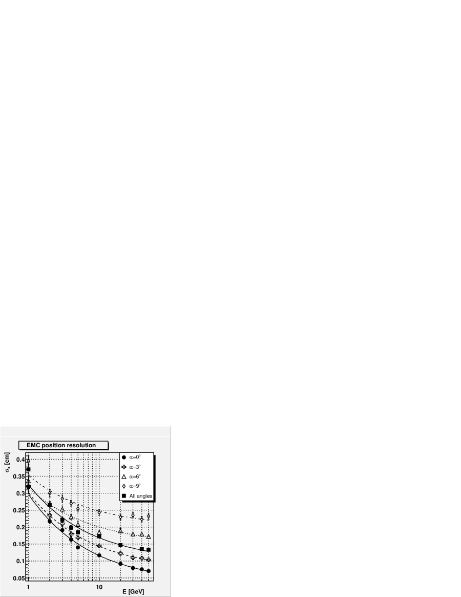
Figure 10: EMC position resolution versus photon energy for the incidence angles $\alpha=0,3,6$ and $9^{\circ}$ as well as for all possible incidence angles of photons emitted from the interaction point.

The CPV detector is sensitive to any particle which initiates an ionization process in the CPV gas volume. Therefore it will detect charged particles with almost any momentum. The only parameter which defines the response of the CPV, is the position resolution of the charged track passing through the detector. The effective spatial resolution of CPV was measured during beam-tests as $\sigma_{x}=0.138$ mm (across the wires) and $\sigma_{z}=0.154$ mm (along the wires). Fig. 11 illustrates the coordinate resolution of the CPV.

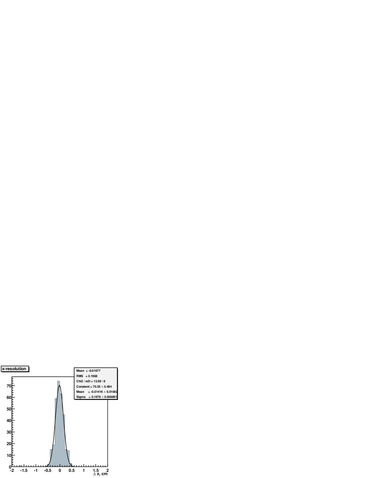
Figure 11: Difference between the exact coordinate of the charged particle impact on the CPV, and the reconstructed coordinate. The plot for the $x$-axis (across the anode wires) is fitted by a single Gaussian, and for the $z$-axis (along the anode wires) is fitted by a sum of two Gaussians.

4.1.3 Particle identification

Particle identification in PHOS is based on three methods:

• Time-of-flight (TOF) of the particles from the interaction point to EMC which allows to discriminate light particles (photons and high-energy hadrons) from slow heavy particles (low-energy nucleons);

• Charge particle rejection which is based on matching of the reconstructed points in CPV and EMC;

• Shower shape analysis which is based on the knowledge of the shower shape produced by different particles in the calorimeter.

The performance of the time-of-flight depends on the time resolution of EMC electronics. The time-of-flight of the photons from the interaction point to PHOS is $15.3$ ns. Figure 12 shows the spectrum of photons compared to those of neutrons and antineutrons identified as photons by TOF with two TOF resolutions, 1 and 2 ns, in the most central Pb-Pb collisions, versus their reconstructed energy in EMC.

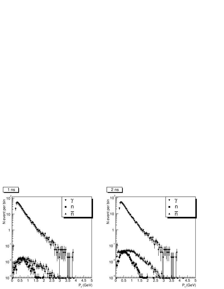
Figure 12: Spectrum of photons, compared to those of neutrons and antineutrons identified as photons by the TOF criterion with two TOF resolutions, 1 (left) and 2 ns (right) in Pb-Pb HIJING events.

The final time resolution for the EMC electronics is not selected yet, so this figure provides the guideline for the design of the TOF system.

Charged particles can be rejected in PHOS if a reconstructed point in the EMC matches a CPV reconstructed point. Figure 13 shows the average deviation between the CPV and EMC reconstructed points for charged pions versus their reconstructed energy, in the ALICE magnetic field 0.5 T.

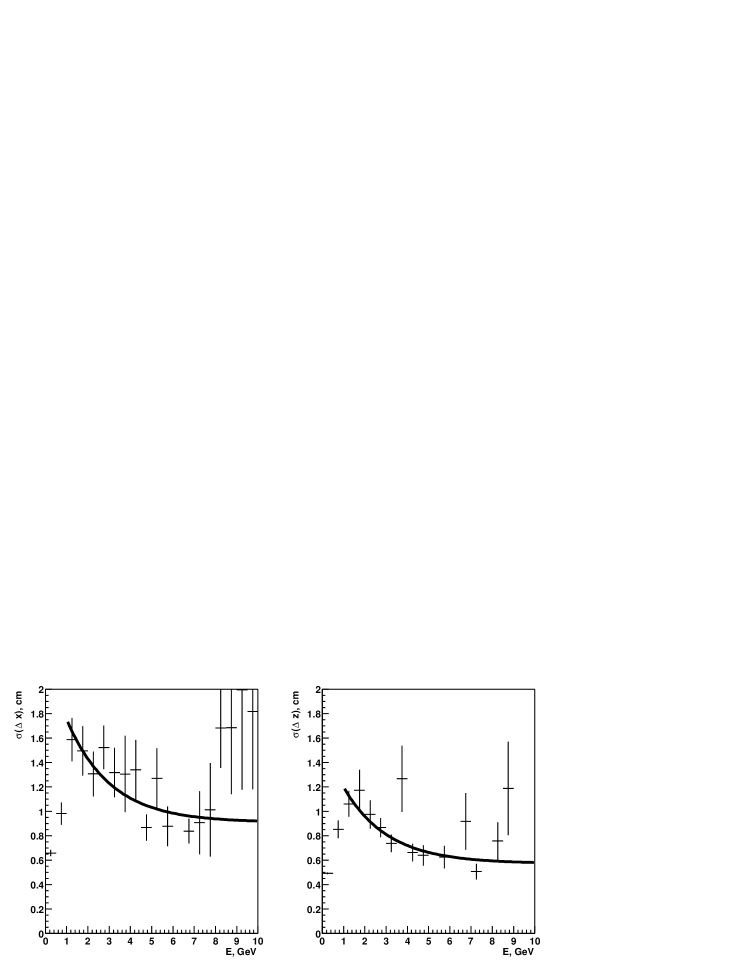
Figure 13: RMS of the Gaussian fit of the EMC-CPV distance along the $x$-axis (i.e. across magnetic field) and $z$-axis (along the beam) for the charged pions produced with a uniform $p_{T}$ distribution versus the deposited energy.

Shower shapes in EMC can be characterized by several parameters. A set of 7 shower parameters has been chosen to identify photons in EMC and discriminate them from hadrons and $\pi^{0}$-mesons:

• lateral dispersion which is a mean squared deviation of the fired cells from the shower center;

• shower main axes, $\lambda_{0}$ and $\lambda_{1}$ which are eigen values of the shower tensor in the $(x,z)$ plane;

• shower sphericity which is a relative difference between $\lambda_{0}$ and $\lambda_{1}$.

• the core energy which is a shower energy within a radius of 3 cm around the shower center;

• the largest energy fraction in a single cell;

• shower cell multiplicity.

These 7 parameters can be statistically correlated, and a set of 7 statistically independent parameters is found by diagonalizing the covariance matrix of the shower shape in this 7-dimensional space.

Figure 14 shows the purity of identified photons by all three identification criteria, as well as the contamination by antineutrons. Purity is a fraction of the reconstructed particles identified as photons, which are really photons, from the total number of reconstructed particles identified as photons. Contamination in defined as a fraction of antineutrons which are identified as photons, from the total number of reconstructed particles and identified as photons particles. The purity and contamination are shown for three definitions of photon quality: low, medium and high purity photons.

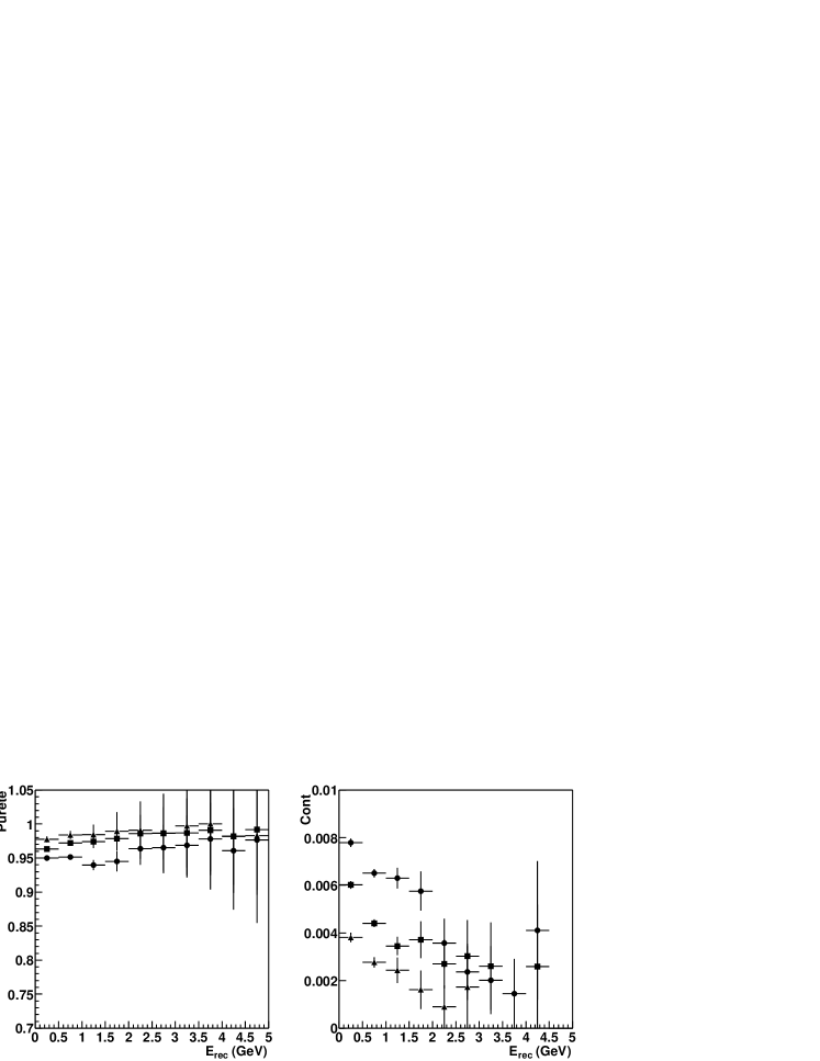
Figure 14: Photon purity and antineutron contamination to the identified photon spectrum in HIJING Pb-Pb collisions, for three definitions of photon quality: low ($\blacktriangle$), medium ($\blacksquare$) and high ($\bullet$) purity photons.

Shower shape analysis allows to distinguish photons and $\pi^{0}$-mesons at high $p_{T}$, where both particles produce a single shower in EMC. Figure 15 shows the true identification probability of a photon at high $p_{T}$, a misidentification probability of a photon as a $\pi^{0}$ and the ratio of the misidentification probability to the true identification probability, for low, medium and high purity photons. This plot clearly illustrates that photons can be distinguished from the $\pi^{0}$-mesons in a wide dynamical range.

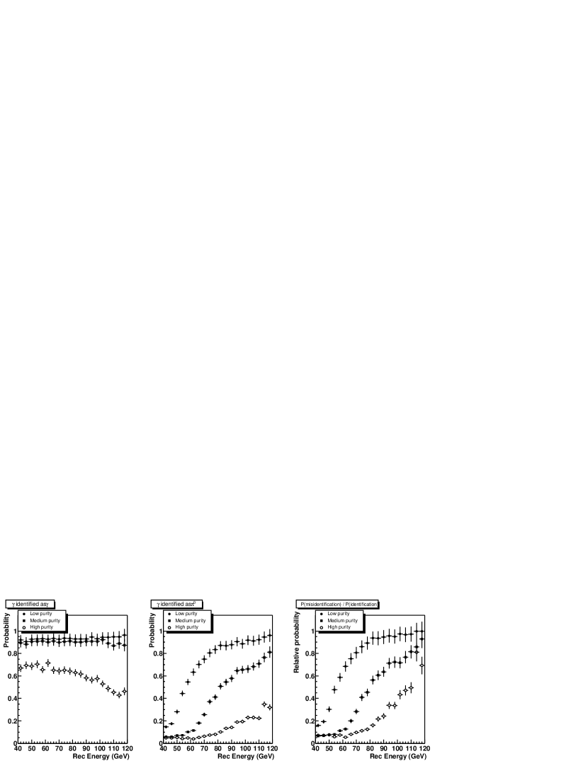
Figure 15: Photon true identification probability, photon misidentification probability as $\pi^{0}$ and the ratio of the misidentification probability to the true one, for three values of photon purities.

4.2 Photon detection at CMS

O.L. Kodolova, J.H. Liu, I.P. Lokhtin, A.N. Nikitenko, I.N. Vardanyan, P. Yepes

4.2.1 CMS detector

The Compact Muon Solenoid (CMS) is a general purpose detector designed primarily to search for the Higgs boson in proton-proton collisions at the LHC [15]. The detector is optimized for accurate measurements of the characteristics of high-energy leptons and photons, as well as hadronic jets in a large acceptance, providing unique capabilities for “hard probes” in both $pp$ and $AA$ collisions [16].

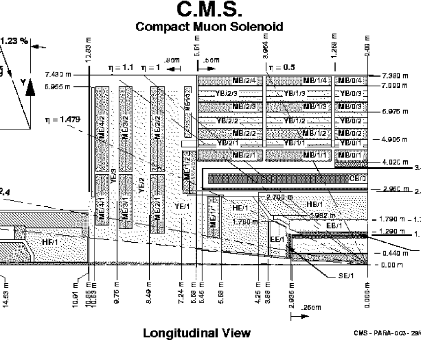
Figure 16: The longitudinal view of the CMS detector.

Detailed description of the detector elements can be found in the Technical Design Reports [17, 18, 19, 20]. The longitudinal view of the CMS detector is presented in Fig. 16. The central element of CMS is the magnet, a $13$ m long solenoid with an internal radius $\approx 3$ m, which will provide a strong $4~{}T$ uniform magnetic field. The $4\pi$ detector consists of a $6$ m long and $1.3$ m radius central tracker, electromagnetic (ECAL) and hadronic (HCAL) calorimeters inside the magnet and muon stations outside. The tracker and muon chambers cover the pseudorapidity region $|\eta|<2.4$, while the ECAL and HCAL calorimeters reach $|\eta|=3$. A pair of quartz-fiber very forward (HF) calorimeters, located $\pm 11$ m from the interaction point, cover the region $3<|\eta|<5$ and complement the energy measurement. The tracker is composed of pixel layers and silicon strip counters. The CMS muon stations consist of drift tubes in the barrel region (MB), cathode strip chambers in the endcap regions (ME), and resistive plate chambers in both MB and ME dedicated to triggering. The electromagnetic calorimeter is made of almost $76000$ scintillating ${\rm PbWO_{4}}$ crystals and the hadronic calorimeter consists of scintillator sandwiched between brass absorber plates. The main characteristics of the calorimeters are presented in Table 2.

Table 2: Energy resolution, $\sigma/E$, and granularity of the CMS calorimeters in the barrel (HB, EB), endcap (HE, EE) and very forward (HF) regions. The energy resolution is shown for the total energy of electrons and photons (ECAL) and transverse energy of hadronic jets (HCAL, HF).

Rapidity coverage	$0<\mid\eta\mid<1.5$		$1.5<\mid\eta\mid<3.0$		$3.0<\mid\eta\mid<5.0$
Subdetector	HCAL (HB)	ECAL (EB)	HCAL (HE)	ECAL (EE)	HF
$\sigma/E=a/\sqrt{E}\bigoplus b$
$a$	1.16	0.027	0.91	0.057	0.77
$b$	0.05	0.0055	0.05	0.0055	0.05
granularity
$\Delta\eta\times\Delta\varphi$	$0.087\times 0.087$	$0.0174\times 0.0174$	$0.087\times 0.087$	$0.0174\times 0.0174$	$0.175\times 0.175$
				to $0.05\times 0.05$

4.2.2 Photon triggering and identification

Photon identification, measurement and triggering in Pb$-$Pb collisions with the maximum estimated particle density, $dN^{\pm}/dy(y=0)=8000$, have been studied [16, 21] with a full GEANT-based simulation of the CMS calorimetry and a parameterization of HIJING [22] data for the background.

The CMS electron/photon trigger algorithm developed for $pp$ collisions, see Fig. 17, is suitable for triggering on energetic photons produced in the heavy ion collisions. Programmable thresholds on the cluster variables used in the algorithm have to be tuned to make it efficient. Estimates of the photon trigger rates have been made with two Algorithm Vetoes, see Fig. 17, the Hadronic Veto ($H/E<0.4$) and Neighbour $E_{T}$ Veto ($\sum_{5}$ Neighbours $E_{T}$ $<25$ GeV). The rate of the single photon trigger is less than $1$ ($10$) Hz for a $50$ ($20$) GeV threshold. With a such a threshold, the trigger efficiency is close to $100\%$ for the $\gamma+$jet events useful for the off-line analysis [21].

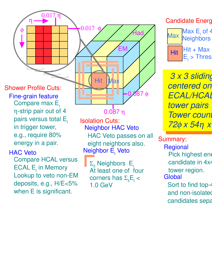
Figure 17: The CMS electron/photon trigger algorithm.

Apart from the trigger selections, single photon identification based on calorimeter isolation or on the use of calorimeter cells above a certain $E_{t}$ threshold (labeled “cell $E_{t}$ cut”) was considered. The photon energy may be measured in a $5\times 5$ crystals cell (the trigger cell size) centred on the crystal with the highest response. Such a cell contains about $97\%$ of the photon energy. Identification may be based on a cut in the transverse energy, $E_{t}^{\rm isol}$, deposited in an area of $3\times 3$ or $5\times 5$ such cells, not including the central one. Distributions of $E_{t}^{\rm isol}(5\times 5)$ and $E_{t}^{\rm isol}(3\times 3)$ are shown in Fig. 18(a) and (b) for the energy from a Pb$-$Pb event deposited in the ECAL only and in the total ECAL$+$HCAL system. Only about $6\%$ of the transverse energy in the isolation area is measured by the hadron calorimeter, reflecting the softness of the charged particle spectra.

The “cell $E_{t}$ cut” criterion is another method of photon identification which has been studied. It requires no energy above a given threshold deposited in every cell of the area around the central cell containing the photon. The transverse energy distribution in the cell is shown for Pb$-$Pb events in Fig. 18(c). A threshold of $E_{T}=6.5$ GeV has been chosen for this distribution. This has been applied in an area of $7\times 7$ cells, not including the central $3\times 3$ trigger matrix since the trigger criteria must still be optimized and applied separately. “Cell $E_{t}$ cut” gives us a rejection factor of $\sim 2.7$ for $\pi^{0}$ decays compared to a $14\%$ reduction of the single photon rate.

The photon energy resolution is degraded due to the large “pile up” contribution in heavy ion collisions. In a $5\times 5$ crystal matrix, we have extra energy deposited, with $\sim 1$ GeV, as seen in Fig. 18(d), so that for a 120 GeV photon, the 0.64% test beam resolution [23] will be degraded to $0.80\%$ due to “pile up”. This photon resolution is still much better than the jet energy resolution. This can be improved by using $3\times 3$ crystals matrix for energy measurement.

4.2.3 Photon reconstruction efficiency and resolutions

The capability of the CMS ECAL to reconstruct photons in heavy ion collisions was investigated in several $E_{T}$ intervals using a standard electromagnetic cluster reconstruction algorithm implemented in CMS object oriented reconstruction package ORCA (version 6). The algorithm looks for crystals with energies above a certain threshold and creates a cluster in a $5\times 5$ crystal matrix. The full GEANT-based simulation of the CMS calorimetry (CMSIM$\_$125 package) responses on single photons and HIJING central Pb$-$Pb event as a background were used in the analysis for the barrel and endcaps.

Photon reconstruction efficiency as a function of photon transverse energy in Pb$-$Pb and $pp$ events is shown in Fig. 20. The estimated photon reconstruction efficiency for Pb$-$Pb collisions appears to be high enough, $\mathrel{\mathchoice{\lower 3.6pt\vbox{\halign{$\mathsurround=0pt\displaystyle\hfil#\hfil$\cr>\crcr\sim\crcr}}}{\lower 3.6pt\vbox{\halign{$\mathsurround=0pt\textstyle\hfil#\hfil$\cr>\crcr\sim\crcr}}}{\lower 3.6pt\vbox{\halign{$\mathsurround=0pt\scriptstyle\hfil#\hfil$\cr>\crcr\sim\crcr}}}{\lower 3.6pt\vbox{\halign{$\mathsurround=0pt\scriptscriptstyle\hfil#\hfil$\cr>\crcr\sim\crcr}}}}80\%$, starting from $E_{T}\sim 15$ GeV. The efficiency dependence on the pseudorapidity is rather weak. The work on improvement of the photon reconstruction algorithm to increase reconstruction efficiency in high multiplicity environment is in progress. The photon spatial resolutions, $\sigma_{\varphi}\sim\sigma_{\eta}\sim 0.005$, are practically the same for $pp$ and Pb$-$Pb collisions and do not depend significantly on the transverse energy. Such spatial resolution is better than $\eta-\varphi$ size of an ECAL cell, $0.0174\times 0.0174$. However, the influence of Pb$-$Pb background on energy resolution is more significant, as shown in Figure 20. At $E_{T}=10$ GeV, the transverse energy resolution degrades strongly in Pb$-$Pb events relative to $pp$, from $2\%$ to $10\%$. The difference decreases with increasing $E_{T}$ and becomes insignificant at $E_{T}\sim 100$ GeV.

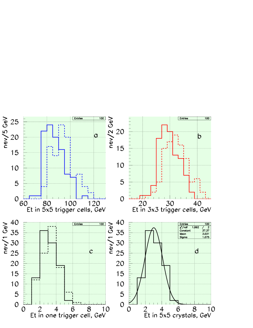
Figure 18: Distribution of the transverse energy of Pb$-$Pb event deposited in trigger cells of $5\times 5$ (a) and $3\times 3$ (b) crystals, not including the central one. (c) The transverse energy deposited in one trigger cell. The solid histograms in (a)-(c) give the energy in the electromagnetic calorimeter while the dashed histograms give the energy in the ECAL$+$HCAL system. (d) A fit of the transverse energy deposited in the electromagnetic part of one trigger cell.

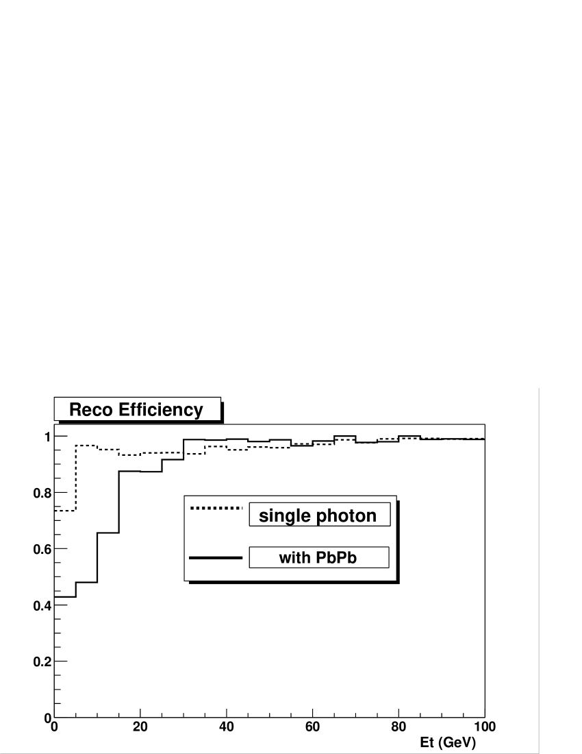
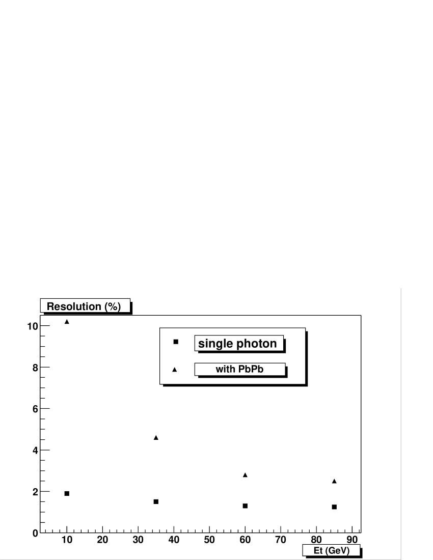
Figure 19: Photon reconstruction efficiency in Pb$-$Pb (solid) and $pp$ (dashed) events.

Figure 20: Photon transverse energy resolution in Pb$-$Pb (triangles) and $pp$ (squares) events.

4.2.4 Jet reconstruction

A detailed description of the jet reconstruction procedure in heavy ion collisions using the sliding window-type jet finding algorithm which subtracts the large background from the underlying event and a full GEANT-based simulation of the CMS calorimetry can be found in the chapter on jets. The efficiencies and background contamination levels are shown in Table 3, along with the transverse energy resolution for several values of jet transverse energy in central Pb$-$Pb collisions assuming $dN^{\pm}/dy(y=0)=8000$. The jet energy resolution is defined as $\sigma(E_{T}^{\rm reco}/E_{T}^{\rm gen})/\langle E_{T}^{\rm reco}/E_{T}^{\rm gen}\rangle$ where $E_{T}^{\rm reco}$ is the reconstructed transverse energy and $E_{T}^{\rm gen}$ is the transverse energy of all generated particles inside the given cone radius $R$. Starting at $E_{T}=100$ GeV, jets can be reconstructed with $100\%$ efficiency and purity. The purity is defined as number of events with true QCD jets divided by the number of events with all reconstructed jets.

Table 3: The jet purity, noise (contamination levels, false jets / generated jets) and transverse energy resolution ($|\eta|<0.3$, $R=0.6$) in central Pb$-$Pb collisions with $dN^{\pm}/dy(y=0)=8000$.

$E_{T~{}{\rm min}}$ (GeV)	Purity	Noise	$\sigma(E_{T})/E_{T}(\%)$
75	0.88 $\pm$ 0.03	0.083 $\pm$ 0.009	17.8
100	0.97 $\pm$ 0.03	0.011 $\pm$ 0.003	18.4
125	0.99 $\pm$ 0.03	0.004 $\pm$ 0.002	16.8
200	0.99 $\pm$ 0.03	0.001 $\pm$ 0.001	12.7

Although the jet transverse energy resolution is degraded by a factor $\sim 2$ in high multiplicity central Pb$-$Pb collisions compared to $pp$, the average measured jet energy in Pb$-$Pb collisions is the same as in $pp$. Thus $pp$ interactions can be used as a baseline for heavy ion jet physics.

It is important to note that the jet angular resolution, $\sigma_{\varphi}=0.045$ and $\sigma_{\eta}=0.05$ at $E_{T}^{\rm jet}=100$ GeV, is still better than the $\eta-\varphi$ size of an HCAL tower $0.087\times 0.087$. Thus the angular position of a hard jet can be reconstructed in heavy ion collisions at CMS with high enough accuracy for analysis of jet production as a function of azimuthal angle and pseudorapidity.

4.3 Photon studies in the ATLAS detector

H.Takai, S. Tapprogge

The ATLAS detector is designed to study high $p_{T}$ physics in full luminosity proton-proton collisions at the LHC. Most of the detector subsystems will be available for heavy ion collisions as well. We are interested in the detection of photons from heavy ion collisions. The highly segmented electromagnetic calorimeter will be heavily used for this studies. We report on early assessment of the detector capabilities in the heavy ion environment.

4.3.1 The ATLAS Detector

The ATLAS detector is designed to study proton-proton collisions at the LHC design energy of 14 TeV in the center of mass. The physics pursued by the collaboration is vast and includes: Higgs boson search, searches for SUSY, and other scenarios beyond the Standard Model, as well as precision measurements of processes within (and possibly beyond) the Standard Model. To achieve these goals at full machine luminosity of $10^{34}cm^{-2}s^{-1}$, ATLAS will have a precise tracking system (Inner Detector) for charged particle measurements, an as hermetic as possible calorimeter system, which has an extremely fine grain segmentation, and a stand-alone muon system. An overview of the detector is shown in Figure 21.

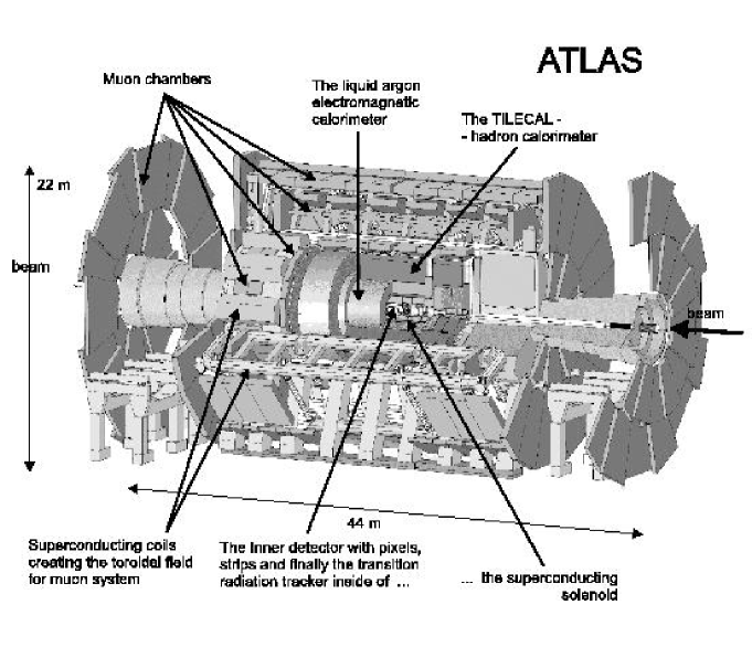
Figure 21: The overall layout of the ATLAS detector

The Inner Detector is composed of (1) a finely segmented silicon pixel detector, (2) silicon strip detectors (Semiconductor Tracker (SCT)) and (3) the Transition Radiation Tracker (TRT). The segmentation is optimized for proton-proton collisions at design machine luminosity. The inner detector system is designed to cover a pseudo-rapidity of $\mid\eta\mid<2.5$ and is located inside a 2 T solenoid magnet.

The calorimeter system in the ATLAS detector that surrounds the solenoid magnet is divided into electromagnetic and hadronic sections and covers pseudo-rapidity $\mid\eta\mid<4.9$. The EM calorimeter is an accordion liquid argon device and is finely segmented longitudinally and transversely for $\mid\eta\mid\leq 3.1$. The first longitudinal segmentation has a granularity of 0.003 x 0.1 $(\Delta\eta\times\Delta\phi)$ in the barrel and slightly coarser in the endcaps. The second longitudinal segmentation is composed of $\Delta\eta\times\Delta\phi=0.025\times 0.025$ cells and the last segment $\Delta\eta\times\Delta\phi=0.05\times 0.05$ cells. In addition a finely segmented $(0.025\times 0.1)$ pre-sampler system is present in front of the electromagnetic (EM) calorimeter. The overall energy resolution of the EM calorimeter as determined in test beam measurements is $10\%/\sqrt{E}\oplus 0.5\%$. The calorimeter also has good pointing resolution, $60mrad/\sqrt{E}$ for photons and timing resolution better than 200 ps for showers of energy larger than 20 GeV.

The hadronic calorimeter is also segmented longitudinally and transversely. Except for the endcaps and the forward calorimeters, the technology utilized for the calorimeter is a lead-scintillator tile structure with a granularity of $\Delta\eta\times\Delta\phi=0.1\times 0.1$. In the endcaps the hadronic calorimeter is implemented in liquid argon technology for radiation hardness with the same granularity as the barrel hadronic calorimeter. The energy resolution for the hadronic calorimeters is $50\%/\sqrt{E}\oplus 2\%$ for pions. The very forward region, up to $\eta=|4.9|$ is covered by the Forward Calorimeter implemented as an axial drift liquid argon calorimeter. The overall performance of the calorimeter system is described in [24].

The muon spectrometer in ATLAS is located behind the calorimeters, thus shielded from most hadronic showers, and has a coverage of $\mid\eta\mid<2.7$. The spectrometer is implemented using several technologies for tracking devices and a toroidal magnet system, which provides a field of 4 T strength to have an independent momentum measurement outside the calorimeter volume. Most of the volume is covered by MDTs (Monitored Drift Tubes). In the forward region, where the rate is high, the Cathode Strip Chamber technology is chosen. The stand-alone muon spectrometer momentum resolution is of the order of $2\%$ for muons with $p_{T}$ in the range 10 - 100 GeV.

The trigger and data acquisition system of ATLAS is a multi-level system, which has to reduce the beam crossing rate of 40 MHz to an output rate to mass storage of $\mathcal{O}(100)$ Hz. The first stage (LVL1) is a hardware based trigger, which makes use of coarse granularity calorimeter data and dedicated muon trigger chambers only. It has to reduce the output rate to about 75 kHz, within a maximum latency of 2.5 $\mu$s. The High-Level Trigger (HLT) is composed of two stages, the second level trigger (LVL2) and the event filter (EF), where further reduction of the rate is achieved using algorithms implemented in software, making use of the full granularity and all sub-detectors. For LVL2, the Region-of-Interest (RoI) concept is used to reduce the amount of event data needed to only a few per cent. For heavy ion physics where an interaction rate of 8 kHz is expected for full luminosity Pb-Pb collisions, we expect to be able to record data with minimal trigger requirements, e.g. centrality trigger.

The performance results mentioned have been obtained using a detailed full simulation of the ATLAS detector response with GEANT and have been validated by an extensive program of testbeam measurements of all components.

4.3.2 ATLAS and Photon physics

Photons in ATLAS are detected in the EM calorimeter. Early in the detector design it was decided to include the capabilities of detecting the Higgs boson through its decay into two photons. Therefore the calorimeter is highly optimized for high $p_{T}$ photon detection and good rejection of $\pi^{0}$’s. The EM calorimeter sampling is divided in fine strips of $\Delta\eta\times\Delta\phi=0.003\times 0.1$ to aid in the $\pi^{0}$ rejection, by identifying overlapping photon showers. Extensive simulations of the performance in proton-proton environment have been carried out. Figure 22 shows the results of this studies for photons with transverse energies up to 100 GeV.

Figure 22: Photon to $\pi^{0}$ rejection as function of $\eta$.

Figure 23: Jet rejection after photon selection cuts as function of jet $E_{T}$ for low and high luminosity proton-proton conditions.

Heavy ion events are different in character when compared to high luminosity proton-proton runs. Although the multiplicity is higher there is no event pile-up. The underlying background to signals of interest, for a typical central collision HIJING event, comes from the soft particles produced in the collision. The majority of the soft charged particle tracks ($p_{T}\leq 200MeV/c$) are curled up in the solenoid magnetic field. At the face of the calorimeter the density of charged particles is approximately $dN/dy\sim 2000$. The neutral particles are in their vast majority low $p_{T}$ $\pi^{0}$s and they will tend to deposit most of their energy in the first compartment, if not in the calorimeter and solenoid cryostat walls ($\sim 1X_{0}$) However, the second electromagnetic compartment could be relatively quiet and used for photon studies.

The major challenge in the study of single photons with the ATLAS detector will be the mis-identification of $\pi^{0}$’s (or jets with a leading $\pi^{0}$) as a photon. Studies performed for high luminosity proton-proton runs indicate good performance for single photon identification. This is shown in Figs. 22 and 23. Because the performance is due to the fine transverse segmentation coupled to a longitudinal segmentation, we do expect similar performance for heavy ions. Detailed simulation studies are under way.

5 NON THERMAL PRODUCTION MECHANISMS

P. Aurenche, F. Bopp, H. Delagrange, S. Jeon, P. Levai, J. Ranft, I. Sarcevic, M. Tokarev, M. Werlen

For the discovery of the quark-gluon plasma using single photon production the $p_{{}_{T}}$ range of interest is roughly 1 GeV/c $<p_{{}_{T}}<$ 10 GeV/c: indeed it is expected that thermal photon production in heavy ion collisions will increase the production rate somewhere in this domain. It is therefore important to also understand the non thermal production mechanism in the same energy range. We shall consider both $\gamma$ and $\pi^{0}$ production since the latter is a background to the former. To calculate the relevant rates the usual theoretical tools at our disposal are the next-to-leading logarithm (NLO) QCD calculations. However, the considered $p_{{}_{T}}$ values are very small compared to the center-of-mass energy of the collision and one is not far from the (small $x$) kinematical boundary where perturbation theory may not be reliable. We therefore supplement the QCD predictions with those from a model which includes soft physics dynamics as well as semi-hard physics: such a model (Dual Parton Model as implemented in Phojet/Dpmjet) has been successfully confronted with data over a wide energy domain. We review each approach in turn, before presenting phenomenological results.

5.1 Theory : perturbative QCD approach at next-to-leading order (NLO)

P. Aurenche, H. Delagrange, S. Jeon, P. Levai, I. Sarcevic, M. Werlen

5.1.1 Proton-proton collisions

The production cross section of a particle at large transverse momentum in perturbative QCD is well known and has the usual factorisable form:

$${d\sigma^{{}^{AB\rightarrow C}}\over d{\tenimbf p_{{}_{T}}}dy}={\sum}_{a,b,c}\int dx_{a}dx_{b}{dz\over z^{2}}F_{{}_{a/A}}(x_{a},M)F_{{}_{b/B}}(x_{b},M)D_{C/c}(z,M_{{}_{F}}){d{\widehat{\sigma}}^{{}^{ab\rightarrow c}}\over d{\tenimbf p_{c}{{}_{{}_{T}}}}dy_{c}}(\mu,M,M_{{}_{F}}),$$ (3)

where the functions $F$ are the parton densities and $\ {\widehat{\sigma}}^{{}^{ab\rightarrow c}}$ is the hard cross section between partons $a$ and $b$, in the hadrons $A$ and $B$ respectively, to produce parton $c$. The function $D_{{}_{C/c}}$ is the fragmentation function of parton $c$ into particle $C$. In the case a photon is produced, an extra term has to be considered where the fragmentation function reduces to a $\delta(1-z)$ function: in this case the photon participates directly to the hard collision ($c=\gamma$) in contrast to the bremsstrahlung process where the photon is produced in the fragmentation of a quark or gluon $c$. The calculations have been carried out up to next-to-leading order [26, 27] in QCD (all functions $F,\ D,\ \sigma^{{}^{ab\rightarrow c}}$ are known in the NLO approximation) but there remains a residual ambiguity related to the choice of the unphysical renormalization scale $\mu$, factorization scale $M$ and fragmentation scale $M_{{}_{F}}$.

For photon production extensive phenomenological studies have been carried out in proton/(anti-)proton scattering for $\sqrt{s}$ from 20 GeV to 1.8 TeV and the situation was found to be rather confused [28, 29, 30]. Concerning results on fully inclusive photon production in $pp$ and $\bar{p}p$, the theory is in satisfactory agreement with all data from (fixed target) 20 GeV to (ISR) 63 GeV with the same set of parameters (all scales set around $p_{{}_{T}}/2$ or slightly smaller). There is one exception: the E706 data [28] (at 31.6 and 38.8 GeV on Beryllium, but corrected by the experimental group to be compared to proton-proton scattering) which are at least a factor 2 to 3 above the other data and which do not have the same $p_{{}_{T}}$ dependence. For $\pi^{0}$ production NLO theory and data are in agreement as far as the shape of the spectrum is concerned but the data are systematically above theoretical predictions [30] (with large fluctuations in the normalization of experiments when compared to theory): one possible explanation is the poor knowledge of fragmentation functions in the dominant large $z$ region which is hardly constrained by $e^{+}e^{-}$ data from which the fragmentation functions are mostly derived. Indeed a large variation in the theoretical rates is observed when using different fragmentation functions (BKK [31], KKP [32], Kretzer [33]). The recent RHIC data at 200 GeV [4] will certainly help clarify the phenomenology.

In the present work, one will need the NLO calculations in a brand new kinematical regime: $\sqrt{s}=5.5$ and $14$ TeV and $p_{{}_{T}}>3$ GeV, corresponding to very small $x$ values. ”Large $p_{{}_{T}}$” NLO calculations have never been tested before, in hadronic collisions, in this small $x$ kinematical regime. For transverse momentum of 3 GeV, the typical $x=2p_{{}_{T}}/\sqrt{s}$ values are of the order of $10^{-3}$ and much less if forward/backward rapidities are explored. One may question the reliability of straightforward NLO calculations in this domain. This is where “recoil” resummation [34] is important but further studies are needed since the present results are rather dependent on non-perturbative parameters and no convenient phenomenological calculations are available at present. As mentioned above the NLO predictions also suffer from the usual (factorization, fragmentation, renormalization) scale uncertainties. In the following we follow the usual (albeit arbitrary) practice to choose a common scale and let it vary between $p_{{}_{T}}/2$ and $2p_{{}_{T}}$. The uncertainties on structure/fragmentation functions will be probed by using different sets.

A specific feature of photon production at very high energy is related to the fact that the bremsstrahlung component becomes large and dominant at small $x$. However this component is not really under control: in particular the $G\rightarrow\gamma$ fragmentation channel is very important but it is not constrained by previous data [35]. This point was not relevant for lower energies because of larger $x$ values or because it was eliminated by isolation cuts in the collider data. However, at LHC, for small $p_{{}_{T}}$ this will introduce a large uncertainty on prompt photon production.

Among other possible uncertainties in the predictions, one should mention those related to the ”intrinsic” $k_{{}_{T}}$. As will be seen below, the $\pi^{0}$ spectrum obtained at RHIC turns out to be in very good agreement with NLO predictions using standard scales (of the order of $p_{{}_{T}}$) thus alleviating the need of introducing ”$k_{{}_{T}}$ effects”.

To summarize: the main uncertainties in the predictions are, as usual, related to the choice of scale values and the choice of fragmentation functions, the latter being important even in the case of prompt photon production because of the importance of the bremsstrahlung mechanism at small $p_{{}_{T}}$ and large energy. As for the uncertainties associated to the structure functions they turn out to be relatively small (a few $\%$ only). These points will be illustrated quantitatively in the phenomenological sections. At a more fundamental level, we must admit that the NLO machinery is applied in a kinematical region where it may not be justified but we have no possibility to gauge the associated uncertainty until recoil resummation is understood, a problem which needs an urgent solution.

5.1.2 Nuclear effects in $p$A collisions

One explains, in Appendix I, how to relate a $p$A hard cross section to the corresponding proton-nucleon cross section [Eqs. (135), (136)]. The incoming proton undergoes multiple scattering on the nucleons, constituents of the nucleus. The number of collisions $N_{coll}$ depends on the value of the impact parameter $b$ or equivalently on the ”centrality class”, a high centrality being obtained in collisions at small impact parameter. The Glauber model used to describe the multiple collisions is based on the eikonal approximation (independent scattering) and it is assumed that the parton distributions of the nucleons, confined in the nucleus, are the same as those of the free nucleon. It is known however that nuclear effects modify the partons distributions. The nuclear structure functions are measured in Deep Inelastic Scattering (DIS) of leptons on nuclei [37]. At small values of $x$, for $x\leq 0.07$, the nuclear structure function is found to be less than nucleon structure function scaled by $A$, exhibiting the so-called nuclear shadowing. As $x$ grows, the nuclear structure function gets bigger than the nucleon structure function. This is known as anti-shadowing. The kinematic region of interest at LHC energies is the region of nuclear shadowing [38].

To calculate the rate of a hard process in proton-nucleus collisions one therefore uses Eq. (3) to describe the proton nucleon collision, where one of the partonic distribution $F_{a/{\rm A}}(x,M)$, say, is a nuclear structure function properly normalized. Due to nuclear shadowing we expect at LHC, a suppression of photon and pion production in proton-nucleus collisions compared to the nucleon-nucleon case. The modification of the parton distribution is written in a factorized form as

$$F_{a/{\rm A}}(x,M)=S_{a/{\rm A}}(x,M)\,F_{a/N}(x,M)$$ (4)

where $F_{a/N}(x,M)$ is the parton distribution function in a nucleon and $S_{a/{\rm A}}(x,M)$ is the parton shadowing function. We assume here $F_{a/{\rm A}}(x,M)$ to be normalized to one nucleon in the nucleus. Recent parametrizations of the shadowing function of Eskola, Kolhinen and Salgado (EKS98), which are $M{~{}}^{2}$ dependent, distinguish between quarks and gluons [39, 40] and are shown to be in very good agreement with the NMC data on $M^{2}$ dependence of $F_{2}^{\rm Sn}/F_{2}^{\rm C}$ [41]. Another parametrization of nuclear parton distributions has been given in [42]. A detailed comparison between these various sets is given in Eskola et al. [38].

In the infinite momentum frame where the nucleus is moving very fast, shadowing is caused by high parton density effects at small $x$. The small $x$ partons have a large longitudinal wavelength and can spatially overlap and recombine. These recombination effects reduce the nuclear parton number densities and hence the nuclear cross sections. Working in this frame enables one to treat nuclear shadowing and parton saturation in nucleons on the same footing due to the identical physical mechanism involved in both. Anti-shadowing is due to longitudinal momentum conservation (momentum sum rule) in this frame.

Even though there has been considerable amount of theoretical work done on nuclear shadowing and impressive progress made in understanding the physical principles of nuclear shadowing [41], we are far from having a precise and quantitative description of nuclear shadowing. The scale dependence of the nuclear structure functions is even less understood due to the limited range of $Q{~{}}^{2}$ covered in fixed target experiments. Also, shadowing of gluons is not well understood due to the fact that they cannot be directly measured in DIS experiments. The working assumption is that high parton density effects are negligible and DGLAP evolution equations are valid in which case the gluon distribution function can be obtained from the scaling violation of the $F_{2}$ structure functions. This assumption, however, will break down at small values of $x$ due to high parton density effects [43] and one will need to measure the gluon distribution function differently.

Another nuclear effect that may be considered is that of the Fermi momentum in the nucleus. In some approaches this contributes an extra nuclear ”$k_{{}_{T}}$” which compounds with the intrinsic ”$k_{{}_{T}}$” in the nucleon, thus leading to an appreciable increase of the cross sections [36]. As there is no need of a nucleon ”$k_{{}_{T}}$” to describe proton-proton collisions, we likewise neglect the small nuclear ”$k_{{}_{T}}$” one may introduce for proton-nucleus collisions.

5.1.3 Nucleus-nucleus collisions

The effect of multiple collisions is treated according to the Glauber model [see Appendix I, in particular Eqs. (135), (136)]. Besides nuclear shadowing discussed in the previous section, an important effect in A+A collisions is the medium induced parton energy loss effect [44]. Fast partons produced in parton-parton collision propagate through the hot and dense medium and through scatterings lose part of their energy [45] and then fragment into hadrons with a reduced energy. While a dynamical study of the parton propagation in a hot and dense medium created in a realistic heavy-ion collision and the modification of the hadronization is most desirable, there is a phenomenological model [46] that takes this effect into account. Given the inelastic scattering mean-free-path, $\lambda_{a}$, the parton type $a$ scatters $n$ times within a distance $\Delta L$ before it escapes the system. The modified fragmentation function, $zD_{\gamma/a}(z,M_{{}_{F}})$ is given in terms of the photon fragmentation function $zD^{0}_{\gamma/a}(z,M_{{}_{F}})$ by [46]

$$zD_{\gamma/a}(z,\Delta L,M_{{}_{F}})=\frac{1}{C^{a}_{N}}\sum_{n=0}^{N}P_{a}(n)\bigg{[}z^{a}_{n}D^{0}_{\gamma/a}(z^{a}_{n},M_{{}_{F}})+\sum_{j=1}^{n}\bar{z}^{j}_{a}D^{0}_{\gamma/g}(\bar{z}^{j}_{a},M_{{}_{F}})\bigg{]}$$ (5)

where $z^{a}_{n}=z/(1-(\sum_{i=0}^{n}\epsilon^{a}_{i})/E_{{}_{T}})$, $\bar{z}_{j}^{a}=zE_{{}_{T}}/\epsilon_{j}^{a}$ and $P_{a}(n)$ is the probability that a parton of flavor $a$ traveling a distance $\Delta L$ in the nuclear medium will scatter $n$ times. It is given by

$$P_{a}(n)=\frac{(\Delta L/\lambda_{a})^{n}}{n!}e^{-\Delta L/\lambda_{a}},$$ (6)

and $C^{a}_{N}=\sum_{n=0}^{N}P_{a}(n)$. The first term in Eq. (5) corresponds to the fragmentation of the leading parton $a$ with reduced energy $E_{{}_{T}}-\sum_{i=0}^{n}\epsilon^{i}_{a}$ after $n$ gluon emissions and the second term comes from the $j$-th emitted gluon having energy $\epsilon^{j}_{a}$, where $\epsilon^{j}_{a}$ is the energy loss of parton $a$ after $j$ scattering. One should keep in mind, however, that Landau-Pomeranchuk-Migdal (LPM) effect in QCD has been derived for static scatterers [45], which may not be suitable approximation in case on hot QGP. One can study the effect of parton energy loss on prompt photon and neutral pion production at the LHC by considering the following cases of parton energy loss [47, 48]: 1) constant parton energy loss per parton scattering, $\epsilon^{~{}a}_{~{}n}=const$, 2) Landau-Pomeranchuk-Migdal energy-dependent energy loss, $\epsilon^{~{}a}_{~{}n}\sim\sqrt{E^{a}_{n}}$ and 3) Bethe-Heitler energy-dependent energy loss, $\epsilon^{~{}a}_{~{}n}\sim E^{a}_{n}$. . Alternative parametrizations of parton energy loss in a hot medium will be considered in Chap. 8 [49].

The energy loss mechanism affects the production of pions and the bremsstrahlung production of photons, but not the production of photons directly emitted from the hard scattering process. One therefore expects a stronger reduction of the $\pi^{0}$ rate than the $\gamma$ rate when going from the nucleon-nucleon collisions to A+A collisions and the ratio $\gamma_{\rm prompt}/\pi^{0}$ should be enhanced in A+A collisions compared to $pp$ collisions.

5.2 Theory: the combined Pomeron and (LO) perturbative QCD approach

F.W. Bopp, J. Ranft

Since, as mentioned previously, the relevant kinematical domain of interest is at rather small $p_{{}_{T}}$ we turn now to the discussion of a model which includes a ”soft” physics component based on Regge theory as well as a ”hard” component based on lowest-order perturbative QCD. This model reproduces soft and semi-hard data on production of hadrons from fixed target energies until 2 TeV. The production of ”prompt” photons is not implemented, while that of ”decay” photons is possible since the radiative decays of hadrons are included in the model.

5.2.1 Proton–proton collisions, the Monte Carlo Event Generator PHOJET

Hadronic collisions at high energies involve the production of particles with low transverse momenta, the so-called soft multiparticle production. The theoretical tools available at present are not sufficient to understand this feature from first QCD principles and phenomenological models are typically applied in addition to pertubative QCD. The Dual Parton Model (DPM) [50] is such a model and its fundamental ideas are presently the basis of many of the Monte Carlo (MC) implementations of soft interactions.

Phojet-1.12 [51, 52] is a modern DPM and perturbative QCD based event generator describing hadron-hadron interactions and also hadronic interactions involving photons. Phojet replaces the original Dtujet model [53], which was the first implementation of this combination of perturbative QCD and the DPM.

The DPM combines predictions of the large $N_{c},N_{f}$ expansion of QCD [54] and assumptions of duality [55] with Gribov’s reggeon field theory [56]. Phojet, being used for the simulation of elementary hadron-hadron, photon-hadron and photon-photon interactions with energies greater than 5 GeV, implements the DPM as a two-component model using reggeon theory for soft interactions and (LO) perturbative QCD for hard interactions. Each Phojet collision includes multiple hard and soft pomeron exchanges, as well as initial and final state radiation. In Phojet perturbative QCD interactions are refered to as hard pomeron exchange. In addition to the model features as described in detail in [57], the version 1.12 incorporates a model for high-mass diffraction dissociation including multiple jet production and recursive insertions of enhanced pomeron graphs (triple-, loop- and double-pomeron graphs).

High-mass diffraction dissociation is simulated as pomeron-hadron or pomeron-pomeron scattering, including multiple soft and hard interactions [58]. To account for the nature of the pomeron being a quasi-particle, the CKMT pomeron structure function [59] with a hard gluonic component is used. These considerations refer to pomeron exchange reactions with small pomeron-momentum transfer, $|t|$. For large $|t|$ the rapidity gap production (e.g. jet-gap-jet events) is implemented on the basis the color evaporation model [60].

For hard collisions Phojet uses the LO parton structure functions GRV98(LO)[61]. All color neutral strings in Phojet are hadronized according to the Lund model as implemented in Pythia [62, 63]. No parton fragmentation functions are needed separately.

Phojet has been extensively tested against data in hadron–hadron collisions [57]. In a number of papers the four experimental LEP Collaborations compare many features of hadron production in $\gamma$ –$\gamma$ collisions to Phojet, a rather good agreement is usually found. Phojet has been checked against practically all data on transverse momentum distributions in $pp$ and $\bar{p}p$ collisions from colliders [64]. In Fig. 24 we plot this comparison. Please note that the points in this Figure are from the Phojet Monte Carlo while the data are represented by lines, fits to the data points.

Figure 24: Transverse momentum distributions of charged hadrons. The results of Phojet (points) are compared to experimental data represented by lines, fitted to the data points. The data at $\sqrt{s}$ = 23 and 53 GeV are from the CERN–ISR [65], the data at 200 GeV are from the UA1 Collaboration [66] and the data at 630 and 1800 GeV are from the CDF Collaboration [67].

5.2.2 Collisions involving nuclei, the Monte Carlo Event Generator  Dpmjet-III

The Dpmjet-III code system [68, 69], is a MC event generator implementing Gribov–Glauber theory for collisions involving nuclei. For all elementary nucleon-nucleon collisions it uses the DPM as implemented in Phojet. Dpmjet-III is unique in its wide range of applications simulating hadron-hadron, hadron-nucleus, nucleus-nucleus, photon-hadron, photon-photon and photon-nucleus interactions from a few GeV up to cosmic ray energies.

Since its first implementations [70, 71, 72] Dpmjet uses the Monte Carlo realization of the Gribov-Glauber multiple scattering formalism according to the algorithms of [73] and allows the calculation of total, elastic, quasi-elastic and production cross sections for any high-energy nuclear collision. This formulation of the Glauber model is somewhat more detailed than the model described in Appendix I. In the model [73] the scattering amplitude is parametrized not only by the inelastic nucleon–nucleon cross–section, but it is parametrized by using ${\sigma}_{tot}$, $\rho$ = ${\bf Re}f(0)_{hN}$/${\bf Im}f(0)_{hN}$ and the elastic slope $a$. ${\sigma}_{tot}$ and $a$ are taken as fitted by Phojet while for $\rho$ a parametrization of experimental data is used. However, parameters needed for the collision scaling of the NLO $\pi^{0}$ and $\gamma$ cross sections ($\sigma_{inel}$, $N_{coll}$) are in very close agreement in Dpmjet with the ones determined in Appendix I. To be consistent we use in direct comparisons between Dpmjet and NLO results always $\sigma_{inel}$ and $N_{coll}$ as determined by Dpmjet. No collision scaling is used by Dpmjet, but of course it is easy to calculate $N_{coll}$ in Dpmjet. Realistic nuclear densities and radii are used in Dpmjet for light nuclei and Woods-Saxon densities otherwise.

During the simulation of an inelastic collision the above formalism samples the number of “wounded” nucleons, the impact parameter of the collision and the interaction configurations of the wounded nucleons. Individual hadron–nucleon interactions are then described by Phojet including multiple hard and soft pomeron exchanges, initial and final state radiation as well as diffraction.

As a new feature, Dpmjet-III allows the simulation of enhanced graph cuts in non-diffractive inelastic hadron-nucleus and nucleus-nucleus interactions. For example, in an event with two wounded nucleons, the first nucleon might take part in a non-diffractive interaction whereas the second one scatters diffractively producing only very few secondaries. Such graphs are prediced by the Gribov-Glauber theory of nuclear scattering but are usually neglected. Further features of Dpmjet-III are a formation zone intranuclear cascade [74] and the implementation of certain baryon stopping diagrams [75].

The Dpmjet-III code and further information are available from the authors. Dpmjet-III and earlier versions like Dpmjet-II have been extensively tested against data in hadron–nucleus and nucleus–nucleus collisions [68, 69, 70, 72]. The code is used for the simulation of cosmic ray showers [76].

The transverse momentum distributions according to Dpmjet are largely determined by the properties of Phojet, which is called for each elementary interaction in Dpmjet. Note, all of these elementary interactions are treated kinematically correctly. All Dpmjet events conserve energy, momentum as well as additive quantum numbers like charge, baryon number and strangeness strictly. Because of an appropriate treatment of soft physics the transverse momentum distributions start at $p_{{}_{T}}$ = 0.

Applying Dpmjet to heavy ion collisions at RHIC the first experience was, that the original hadron multiplicities and pseudorapidity distributions were about one third too high compared to the data. A new mechanism was needed to reduce $N_{\rm ch}$ and $dN_{\rm ch}/d\eta|_{\eta=0}$ in situations with a produced very dense hadronic system. Such a mechanism, the fusion and percolation of soft chains, had indeed been conjectured since the beginning of the Nineties. Introducing percolation and fusion of soft chains into Dpmjet[77], it was indeed possible to get a satisfactory agreement of Dpmjet with the $N_{\rm ch}$ and $dN_{\rm ch}/d\eta$ measured at RHIC. The procedure desribed in [77] is quite time consuming and therefore not well suited for high statistics Dpmjet runs as needed here. Therefore, we apply here only an effective method, reducing $N_{\rm ch}$ and $dN_{\rm ch}/d\eta$ in Dpmjet like in [77] without spoiling energy–momentum conservation. This method would not distort the transverse momentum distributions, but it will reduce the cross sections at all $p_{{}_{T}}$ by approximately the same 30 % as mentioned above.

Calculating from Dpmjet transverse momentum distributions of decay photons (Dpmjet or Phojet do not calculate direct photon production) we use the possibility in the code to declare certain resonances as stable. In this way we get separately (i) all decay photons (having $\pi^{0}$ and $\eta$ decaying), (ii) all decay photons not coming fron $\pi^{0}$ decay (declaring $\pi^{0}$ as stable) and (iii) all decay photons not coming from $\pi^{0}$ or $\eta$ decay (declaring $\pi^{0}$ and $\eta$ as stable).

5.3 The $z-$scaling model

M. Tokarev

During the workshop, a phenomenological model to describe hadron and photon production was also discussed: the $z-$scaling model. This concept was suggested to analyze numerous experimental data on high-$p_{{}_{T}}$ hadron production in $pp,\bar{p}p$ and $p$A collisions [78]. The method of data analysis was developed for description of $pp$, $\bar{p}p$ and $p$A interactions with direct photon and jet production in the high-$p_{{}_{T}}$ region at the RHIC and LHC energies as well [79]. The scaling function is expressed via the invariant differential cross section $Ed^{~{}3}\sigma/dp^{3}$ as follows

$$\psi(z)=-\frac{\pi s}{\rho\sigma_{in}}J^{-1}E\frac{d^{3}\sigma}{dp^{3}}.$$ (7)

Here $s$ is the collision center-of-mass energy squared, $\sigma_{in}$ is the inelastic cross section, $J$ is the corresponding Jacobian, and $\rho=dN/d\eta$ is the particle multiplicity density. The function $\psi(z)$ is normalized:

$$\int_{z_{min}}^{\infty}\psi(z)dz=1.$$ (8)

The relation allows us to give the physical meaning of the scaling function $\psi(z)$ as a probability density to form a particle with the formation length. The variable $z$ can be written in the form

$$z=z_{0}\Omega^{-1},\hskip 14.22636pt{\rm{where}}\hskip 28.45274pt\Omega(x_{1},x_{2})=(1-x_{1})^{\delta_{1}}(1-x_{2})^{\delta_{2}}.$$ (9)

The factor $z_{0}$ is proportional to the transverse energy released in the underlying collision of constituents. The expression $\Omega^{-1}$ describes the resolution at which the collision of the constituents can be singled out of this process. The $\Omega(x_{1},x_{2})$ represents the relative number of all initial configurations containing the constituents which carry fractions $x_{1}$ and $x_{2}$ of the incoming momenta. The $\delta_{1}$ and $\delta_{2}$ are the anomalous fractal dimensions of the colliding objects (hadrons or nuclei). The momentum fractions $x_{1}$ and $x_{2}$ are determined in a way to minimize the resolution $\Omega^{-1}(x_{1},x_{2})$ of the fractal measure $z$ with respect to all possible sub-processes which satisfies 4-momentum conservation law.

Figure 25 shows the data $p_{{}_{T}}$ and $z$-presentation for $\pi^{0}$ meson production in $pp$ collisions. The first one demonstrates the strong energy dependence of the cross section as a function of the transverse momentum. The $z$-presentation reveals the energy independence of $\psi(z)$ and, for large enough $z$, the power behavior, $\psi(z)\sim z^{-\beta}$, of the scaling function. Based on the obtained results [78, 79] we can conclude that verification of the asymptotic behavior of $\psi(z)$ for $\pi^{0}$ meson, direct photon and jet production at LHC energies is of interest.

a)                                                              b)

Figure 25: (a) Dependence of the inclusive cross section of $\pi^{0}$ meson production on transverse momentum in $pp$ collisions at $\sqrt{s}=30-200~{}GeV$. Experimental data are obtained at ISR and RHIC. (b) The corresponding scaling function.

Since no predictions are available for A+A collisions we do not pursue the $z-$scaling approach further in this report.

In the next sections of this chapter we compare the model predictions to the $\pi^{0}$ transverse momentum distributions obtained at RHIC at $\sqrt{s}$ = 200 GeV, and then make predictions for $\pi^{0}$ and $\gamma$ spectra at LHC energies. It is found that both Dpmjet and NLO QCD agree with the data and, furthermore, they give very similar results for the extrapolation to LHC energies. A word of warning is necessary at this point concerning the comparison between the two models in nucleus-nucleus collisions . We note that the Dpmjet predictions represent the full picture of a heavy ion collision while the NLO QCD predictions give a partial picture to which the contribution of the quark-gluon plasma should be added (see Chap. 6). In Chap. 6 it is found that thermal contributions, in A+A collisions, are important in the low $p_{{}_{T}}$ range only. Comparing the predictions of the two models for A+A collisions at LHC is therefore relevant only for $p_{{}_{T}}>10-15$ GeV/c. A detailed discussion of our results in A+A collisions below this value of $p_{{}_{T}}$ is given in Chap. 7.

5.4 Phenomenology of $\pi^{0}$ production

Our standard NLO predictions are obtained using the CTEQ5M [80] or, equivalently, CTEQ6M  [81] parton distributions and the KKP [32] fragmentation functions. In Fig. 26, the experimental $\pi^{0}$ transverse momentum spectrum in $pp$ collisions at 200 GeV [4] is compared to theoretical predictions. One notes the remarkable agreement of the data with the NLO QCD estimates as well as with the Dpmjet predictions. The Dpmjet model parameters had been tuned to fit charged particle spectra (see Fig. 24) and no new adjustement was necessary to obtain the $\pi^{0}$ spectrum.

The spread in the NLO QCD estimates (grey band in the figure) reflects the uncertainties associated to the choice of scales (all scales equal varying from .5 $p_{{}_{T}}$ to 2 $p_{{}_{T}}$): if the uncertainty is roughly [$+100\%,\ -60\%$] at $p_{{}_{T}}=3$ GeV/c it reduces to $\pm$ 40% at $p_{{}_{T}}=12$ GeV/c. The upper limit of the NLO predictions is obtained with the smallest scales and the lower limit with the largest scales. Varying the scales independently (for example $\mu=M\neq M_{{}_{F}}$) one still obtains results in the grey band of the figure with only slight changes in the slope in $p_{{}_{T}}$ (for $p_{{}_{T}}$ below 6 GeV/c). Using the BKK [31] fragmentation functions rather than the KKP lowers the theoretical predictions by about 25% while the Kretzer [33] functions reduce the predictions by about 70% (lowest $p_{{}_{T}}$) to 45% (highest $p_{{}_{T}}$). Concerning CTEQ6M, the 40 different sets predict cross sections within $[-5\%,+3\%]$ for $p_{{}_{T}}<10$ GeV/c and within $[-6\%,+10\%]$ at $p_{{}_{T}}=14$ GeV/c. Turning now to MRS99 [82] rather than CTEQ hardly makes any changes: decrease of the cross section by about 10% at low $p_{{}_{T}}$ and stability for $p_{{}_{T}}>6$ GeV/c.
From this discussion one concludes that the largest uncertainties in the theoretical predictions are related to the choice of scales and to the fragmentation functions, a remark which also holds true at LHC energies. Concerning the fragmentation functions, it should be recalled that KKP give the best phenomenology for $\pi^{0}$ production at lower energies [83, 84].

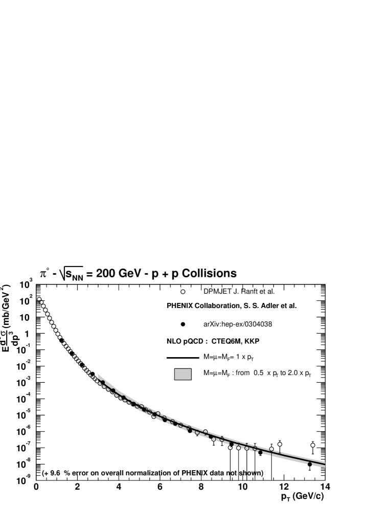
Figure 26: PHENIX data on $\pi^{0}$ production in $pp$ collisions at 200 GeV, compared to various theoretical predictions. The grey band indicates the range the NLO QCD predictions for scales ranging from 0.5 $p_{{}_{T}}$ to 2 $p_{{}_{T}}$ and the open points are the Dpmjet predictions. CTEQ6 [81] structure and KKP [32] fragmentation functions are used. The theoretical predictions are evaluated by averaging the invariant cross sections in an interval $\pm 0.35$ unit of rapidity around rapidity 0.

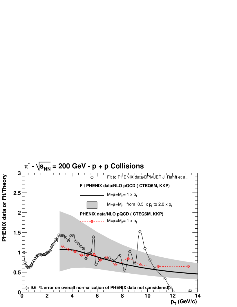
Figure 27: PHENIX data on $\pi^{0}$ production in $pp$ collisions at 200 GeV normalized to various theoretical predictions shown in Fig. 26. The experimental error bars on the data points (crosses) are not shown.

We also show on a linear plot, in Fig. 27, the data normalized to the theoretical predictions. The solid line shows the ratio of a fit of the PHENIX data to the standard NLO predictions while the dashed line, with open crosses, shows the data normalised to the NLO estimates: the agreement between theory and experiment is remarkable given the fact that no parameters has been adjusted to fit the data. In view of the high quality, and large $p_{{}_{T}}$ coverage, of the RHIC present and forthcoming data it would be interesting to perform a joint fit of $e^{+}e^{-}$ data and RHIC data to better constrain the fragmentation functions specially in the high $z$ region where $z$ is the fragmentation variable. Another advantage would be the possibility to obtain a better control on the gluon fragmentation function which appears as a next-to-leading effect in $e^{+}e^{-}$ while it is a leading term in $pp$ collisions: this would help un-correlate the gluon fragmentation parameters from the other parameters in the fit. The agreement between data and Dpmjet is also excellent even at the lowest $p_{{}_{T}}$ values. The large fluctuations at high $p_{{}_{T}}$ are related to the low statistics of the model.

We turn now to LHC energies. The theory predictions are shown, for $pp$ collisions, at 5.5 TeV (Fig. 28) and 14 TeV (Fig. 29). In each case we display two plots, the first one with log-log scales to emphasis the low $p_{{}_{T}}$ region and the other one with semi-log scales up to $p_{{}_{T}}=100$ GeV/c.

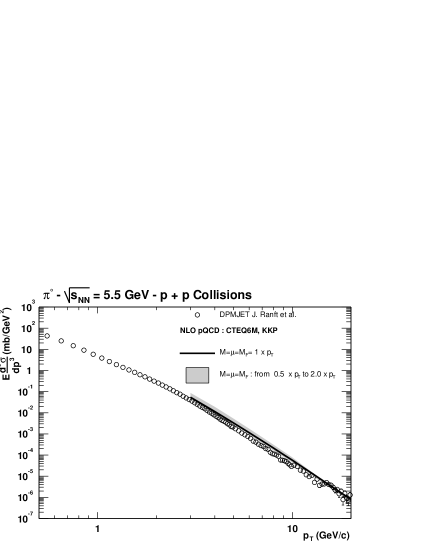
Figure 28: Theoretical predictions for the $\pi^{0}$ transverse momentum spectrum at 5.5 TeV. The conventions used are as in Fig. 26. The invariant cross section is calculated at 0 rapidity.

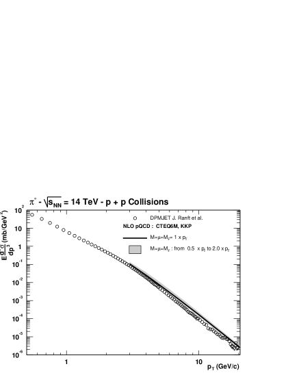
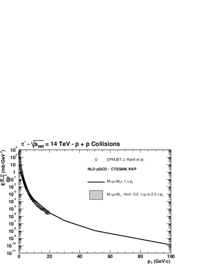
Figure 29: Same as Fig. 28 but at $\sqrt{s}=14$ TeV.

One notes again the good overall agreement between Dpmjet and NLO QCD results in the overlapping region. Furthermore the use of NLO calculations appears reasonable down to $p_{{}_{T}}=3$ GeV/c below which one does not dare make perturbative QCD predictions! In fact, at $p_{{}_{T}}=3$ GeV/c, one notes a change of slope in the Dpmjet predictions, illustrating the effects of soft physics (pomeron exchanges) in the model: the slope of the distribution decreases leading to a finite prediction at $p_{{}_{T}}=0$.

The scale variations in the NLO QCD predictions are still rather large at low transverse momentum (for $p_{{}_{T}}=3$ GeV/c it is [$+60\%,\ -25\%$] at $\sqrt{s}=5.5$ TeV and [$+25\%,\ -20\%$] at $\sqrt{s}=14$ TeV) but reduces to roughly $\pm 10\%$ at $p_{{}_{T}}=100$ GeV/c for both energies. These NLO results tend to be slightly less steep than the Dpmjet prediction and larger even when choosing the largest scales. This is due to using different input parameters for the perturbative sector in the two calculations. Keeping with the CTEQ family of 40 parametrizations the NLO predictions agree within $\pm 10\%$ at $p_{{}_{T}}=3$ GeV/c and within $\pm 2.5\%$ at $p_{{}_{T}}=100$ GeV/c. As mentioned above using MRS99 and BKK fragmention functions would lower the NLO predictions which would then overlap the Dpmjet ones. A power behavior of the predictions holds for $p_{{}_{T}}$ between 3 GeV/c and 20 GeV/c: one finds for Dpmjet a behavior of type

$${d\sigma^{\pi^{0}}\over d{\tenimbf p_{{}_{T}}}dy} \sim {1\over p_{{}_{T}}^{5.91}},\ {\mbox{\rm at 5.5~{}TeV}}$$ (10)

$$\sim {1\over p_{{}_{T}}^{5.63}},\ {\mbox{\rm at 14~{}TeV}},$$ (11)

while for the standard (CTEQ6M, KPP, all scales equal to $p_{{}_{T}}$) NLO predictions the behavior is slightly harder:

$${d\sigma^{\pi^{0}}\over d{\tenimbf p_{{}_{T}}}dy} \sim {1\over p_{{}_{T}}^{5.45}},\ {\mbox{\rm at 5.5~{}TeV}},$$ (12)

$$\sim {1\over p_{{}_{T}}^{5.09}},\ {\mbox{\rm at 14~{}TeV}}\ .$$ (13)

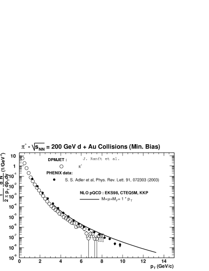
Figure 30: The pion transverse momentum spectrum for deuterium-gold collisions at $\sqrt{s}=200$ GeV. The solid line represents the standard NLO predictions using the EKS shadowing parametrization. The theoretical predictions are evaluated by averaging the invariant cross sections in an interval $\pm 0.35$ unit of rapidity around rapidity 0.

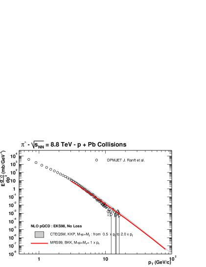
Figure 31: The pion transverse momentum spectrum at $\eta=0$ for proton-lead collisions at $\sqrt{s}=8.8$ TeV. The grey band represents the standard NLO predictions as in previous figures. The solid line is the NLO QCD result using MRS99 [82] and BKK [31] parametrizations with all scales equal to $p_{{}_{T}}$. All NLO predictions include EKS [39, 40] shadowing.

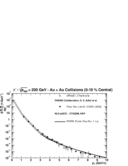
Figure 32: Comparison between PHENIX data on gold-gold collisions at $\sqrt{s}=$ 200 GeV and theoretical predictions. The theoretical predictions are evaluated by averaging the invariant cross sections in an interval $\pm 0.35$ unit of rapidity around rapidity 0.

We consider now deuterium-gold scattering at 200 GeV and proton-lead scattering at $\sqrt{s}=8.8$ TeV and we display, in figs. 30 and 31, the Dpmjet results together with the NLO QCD predictions, using the shadowing model of [39, 40]. At RHIC the agreement between data and the standard NLO predictions is good although the latter may not be steep enough and tend to fall above the data for $p_{{}_{T}}>7$ Gev/c. The magnitude of uncertainties of the NLO calculations is the same as for $pp$ collisions. The Dpmjet predictions have the right order of magnitude at low $p_{{}_{T}}$ but they tend to decrease somewhat too fast as $p_{{}_{T}}$ increases. Work is in progress to understand this point [85].

For LHC in $p$Pb collisions the two models are compatible within the error bars but the slope of the cross section is slightly steeper for Dpmjet. As before the grey band shows the range of predictions for our standard inputs while the solid line is obtained using MRS99 and BKK functions with all scales equal to $p_{{}_{T}}$. The latter result is equivalent to the standard one with all scales equal to $2p_{{}_{T}}$.

Turning now to A+A collisions, the comparison of the $\pi^{0}$ spectrum in gold-gold collisions at $\sqrt{s}=200$ GeV together with the theoretical estimates is shown in Fig. 32. The agreement between theory and experiment is surprisingly good over the whole $p_{{}_{T}}$ range. In the DPM approach no jet quenching and no shadowing are introduced but a string fusion mechanism is at work which is calibrated to reproduce the particle multiplicity. It also reproduces the minimum bias rapidity distributions. In the NLO QCD approach the theory is consistent with the data at large $p_{{}_{T}}$ provided a jet energy loss mechanism is introduced. In the figure we display the result with model 3) of sec. 5.1.3, i.e. Bethe-Heitler energy loss with $\epsilon^{~{}a}_{~{}n}=0.05E^{a}_{n}$ for gluons and $\epsilon^{~{}a}_{~{}n}=0.025E^{a}_{n}$ for quarks and with $\lambda_{a}=0.5$ for gluons and 1 for quarks [47, 48] (see Eq. (6) and the discussion following it). Below $p_{{}_{T}}=5$ GeV/c the NLO QCD predictions fall below the data: this is the region where thermal production of $\pi^{~{}0}$ may become relevant as will be discussed in Chapters 6 and 7.

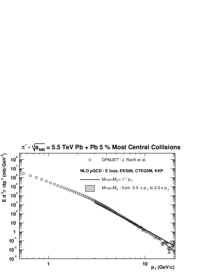
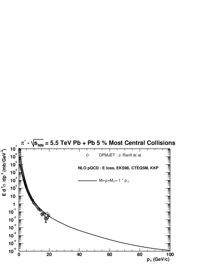
Figure 33: Same as Fig. 28 for lead-lead collisions at $\sqrt{s}=5.5$ TeV.

The extrapolation to lead-lead collisions at $\sqrt{s}=5.5$ TeV are compatible (see Fig. 33) even though the treatment of final state effects in both models is completely different. The Dpmjet results are slightly steeper and one finds, in the range 3 $<p_{{}_{T}}$ [GeV/c] $<$ 20,

$${d\sigma^{\pi^{0}}\over d{\tenimbf p_{{}_{T}}}dy} \sim {1\over p_{{}_{T}}^{5.66}},\ {\mbox{\rm for NLO QCD}}$$ (14)

$$\sim {1\over p_{{}_{T}}^{6.24}},\ {\mbox{\rm for {Dpmjet}}}\ ,$$ (15)

At $p_{{}_{T}}=$ 5 GeV/c one expects, integrated over azimuthal angle and per unit of rapidity, 160 events/${\mbox{\rm GeV}}^{~{}2}$/sec.

5.5 Phenomenology of prompt and decay photon production

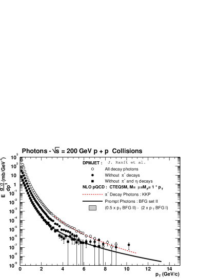
Figure 34: Comparison of “prompt” and “decay” spectra in $pp$ collisions at 200 GeV. CTEQ5 [80] structure functions are used for the NLO QCD predictions. For the prompt photon spectrum the BFG [35] parametrization of fragmentation functions is used while the KKP [32] fragmentation functions are used for the NLO QCD estimates of decay photons. The theoretical predictions are evaluated by averaging the invariant cross sections in an interval $\pm 0.35$ unit of rapidity around rapidity 0.

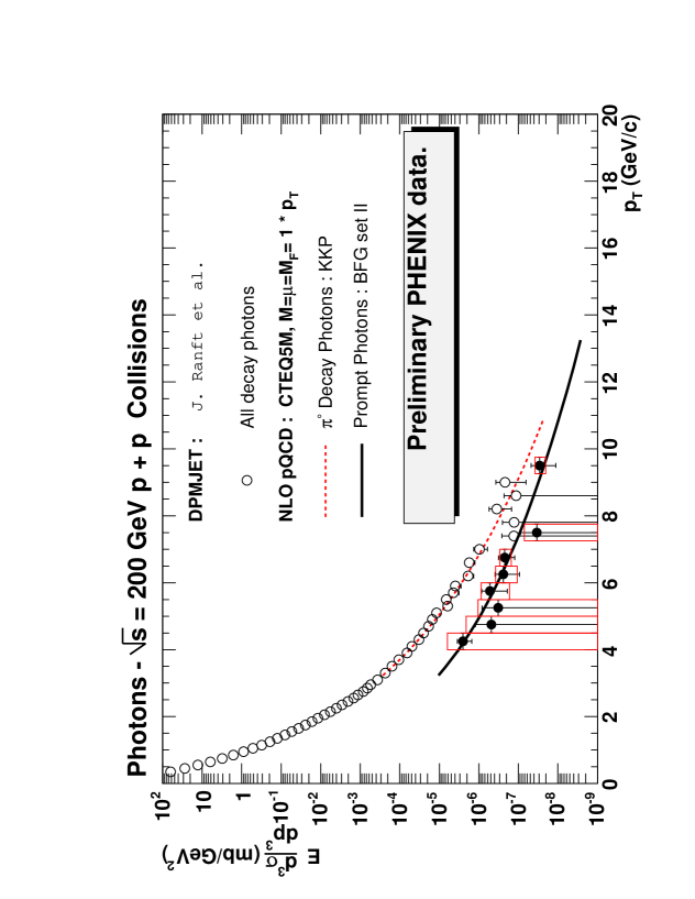
Figure 35: Comparison of the theoretical prompt photon spectrum in $pp$ collisions at 200 GeV, shown in the above figure, with the preliminary PHENIX data (full dots). The data points are collected from a figure shown in ref. [87]. The theoretical predictions of decay photons are those of Fig. 34.

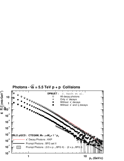
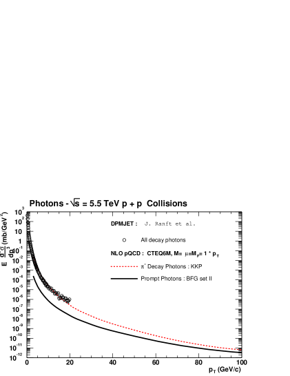
Figure 36: Comparison of “prompt” and “decay” spectra in $pp$ collisions at $\sqrt{s}=$5.5 TeV. CTEQ6 [81] structure functions are used for the NLO QCD predictions. For the prompt photon spectrum the BFG [35] parametrization of fragmentation functions is used while the KKP [32] fragmentation functions are used for the NLO QCD estimates of decay photons. The cross section is evaluated at 0 rapidity.

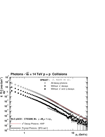
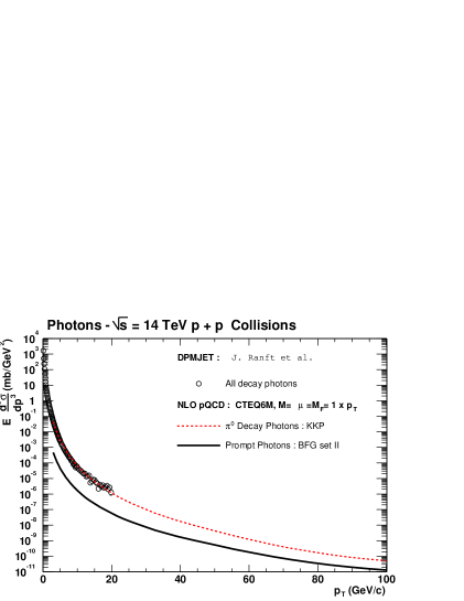
Figure 37: Same as Fig. 36 at $\sqrt{s}=$ 14 TeV.

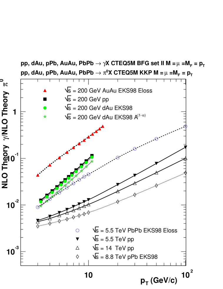
Figure 38: NLO QCD predictions for the ratio $\gamma_{\rm prompt}/{\pi^{0}}$ in proton-proton, proton-nucleus and nucleus-nucleus collisions at 200 GeV and 5.5 TeV. The Au+Au ratio at $\sqrt{s}=$ 200 GeV and the Pb+Pb ratio at $\sqrt{s}=$ 5.5 TeV are modified by thermal effects at the lower $p_{{}_{T}}$ end of the spectrum and are predicted to be higher than shown (see sec. 7.2).

In this section we discuss the photon spectrum and compare the rates of production of “prompt” and “decay” photons. While for $\pi^{0}$ production we have two independent models at our disposal, for the prompt photon spectrum one can, at the moment, only obtain NLO QCD predictions . For decay photons the Dpmjet code explicitely includes the radiative decay of resonances ($\pi^{~{}0}$, $\eta$ and other hadronic resonances of the low mass meson and baryons multiplets) so that one will be able to assess the importance of various channels to the decay photon spectrum. One can also obtain a prediction for the full decay photon spectrum from NLO QCD via standard convolution formulae based on the $\pi^{~{}0}$ spectrum. Assuming a power behavior for the $\pi^{0}$ spectrum, ${d\sigma^{\pi^{0}}/dp_{{}_{T}}}\sim p_{{}_{T}}^{-n}$, one can derive the following formula for the ratio of the decay photon spectrum over the $\pi^{0}$ spectrum [86]:

$$R_{\gamma_{\rm decay}/\pi^{0}}={2\over n-1}.$$ (16)

No isolation cuts have been applied when calculating the photon rates.

The results are displayed in figs. 34 to 41. In all figures, the solid line indicates the “standard NLO QCD” prompt photon predictions based on CTEQ5M or CTEQ6M for the structure functions and BFG set II [35] for the fragmentation functions of partons into a photon. Using (the less favored but still compatible with present data) BFG set I [35] would lower the predictions. The grey band, when shown, indicates the range of uncertainties in the NLO calculations: the lowest prediction is obtained with BFG set I and all scales set to 2 $p_{{}_{T}}$ while the highest one is obtained with BFG set II and all scales set to 0.5 $p_{{}_{T}}$. For the decay photon spectra, we show as a dashed line the estimates of NLO QCD using a generalization of Eq. (16) [86]. Concerning the Dpmjet predictions, the open circles indicate the full photon decay spectrum, the full circles the spectrum with the $\pi^{0}$ decay contribution removed and the full squares the spectrum with both $\pi^{0}$ and $\eta$ decays removed.

At $\sqrt{s}=$ 200 GeV, one sees that the decay photon spectrum dominates the prompt photon one and, furthermore, one notices the excellent agreement between the Dpmjet and the NLO QCD estimates which is not surprising since both models agreed very well in their $\pi^{0}$ spectrum predictions. The range of uncertainties, due to changes of scales and of photon fragmentation functions, in the NLO QCD rate of prompt photons is less than $\pm$ 50% at low $p_{{}_{T}}$ and much smaller at high $p_{{}_{T}}$. Displayed in Fig. 35 is the comparison between the theoretical predictions of prompt photon production and the experimental results recently obtained by the PHENIX collaboration [87]: the agreement is very satisfactory.

At LHC, Figs. 36 and 37, the same features are found except that the prompt photon rate is relatively smaller, at the level of the decay photon spectrum with the $\pi^{0}$ and $\eta$ contributions removed. At low $p_{{}_{T}}$, the uncertainty in the prompt photon spectrum is largely due to the choice of photon fragmentation functions: for $\sqrt{s}=$ 5.5 TeV or 14 TeV, using BFG set I [35] decreases the predictions by a factor of up to $2.5$ at $p_{{}_{T}}\sim$ 3 GeV/c, where the bremsstrahlung component is important, but by $10\%$ or less for $p_{{}_{T}}$ above $20$ GeV/c: this large variation at low $p_{{}_{T}}$ is associated to uncertainties in the gluon fragmentation into a photon which is hardly contrained by present data. At LHC the uncertainty associated to the CTEQ structure functions is much smaller: $\pm 10\%$ at $p_{{}_{T}}=3$ GeV/c and about $\pm 2.5\%$ at $p_{{}_{T}}=100$ GeV/c similarly to the results for $\pi^{0}$ production. As for predictions based on the MRS99 parametrization, they are reduced by less than $15\%$ compared to our standard results, with the largest reduction occuring at the small values of transverse momentum.

In more details, the results for $pp$ scattering at LHC can be summarized as follows: 1) at the lower end of the spectrum, there is almost 10 times more photons from $\pi^{0}$ decays than from all other sources taken together; 2) decays from $\eta$’s are again about 10 ten times larger than those from “other” resonances; 3) the level of production of prompt photon is similar to that of decay photons from “other” hadronic resonances.

At RHIC as well as at LHC, the ratio $\gamma_{\rm prompt}/\gamma_{\rm decay}$ slowly increases with $p_{{}_{T}}$. To see this it is customary to display the ratio $\gamma_{\rm prompt}/{\pi^{0}}$: this is done in Fig. 38 where the predictions for RHIC and LHC are compared. The ratios are rather small, specially at LHC, and isolation cuts will certainly be necessary to increase them.

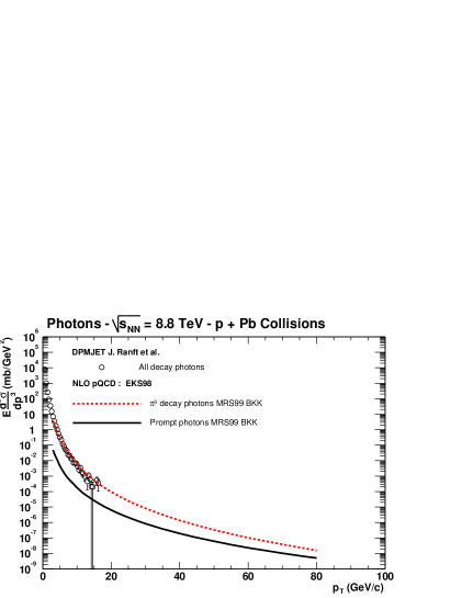
Figure 39: Comparison of “prompt” and “decay” spectra in proton-lead collisions at 8.8 TeV.

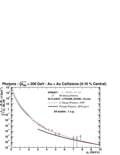
Figure 40: Comparison of the prompt and the decay photon spectra in Au+Au collisions at $\sqrt{s}=200$ GeV in NLO QCD. The Dpmjet results for decay photons are also shown. The theoretical predictions are evaluated by averaging the invariant cross sections in an interval $\pm 0.35$ unit of rapidity around rapidity 0.

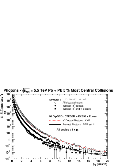
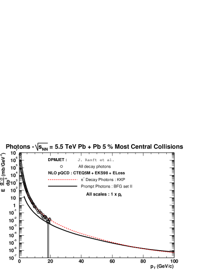
Figure 41: Comparison of “prompt” and “decay” spectra in lead-lead collisions at 5.5 TeV.

In Fig. 39 the results for $p$Pb scattering at LHC are summarized: the Dpmjet predictions are in good agreement with the NLO QCD estimates based on the MRS99 and BKK parametrizations, although they tend to have a slightly steeper slope as already noticed in Fig. 31 for pion production. As expected the prompt photon signal is much below the decay photon spectrum.

The ratio $\gamma_{\rm prompt}/{\pi^{0}}$ is shown in Fig. 38 for $d$Au collisions at 200 GeV and $p$Pb collisions at 8.8 TeV. At RHIC very little change is seen compared to $pp$ collisions at the same energy. We also looked at the effect of assuming an $A^{1-\alpha}$ dependence of the $d$Au cross sections, with $\alpha=1.08$ for $\pi^{0}$ production and $\alpha=1.04$ for $\gamma$ production. It is seen to have a moderate effect on the estimate of the ratio. For $p$Pb scattering at LHC a small energy dependence is observed compared to $pp$ scattering at 5.5 TeV with a larger decrease of the ratio at the larger $p_{{}_{T}}$ values.

We turn finally to the case of nucleus-nucleus collisions. The results for RHIC are shown in Fig. 40. One sees that in Au+Au collisions the ratio $\gamma_{\rm prompt}/\gamma_{\rm decay}$ increases with $p_{{}_{T}}$ and approaches 1 at $p_{{}_{T}}=10$ GeV/c. The value of this ratio is much higher than for $pp$ scattering at the same energy. In the NLO QCD model this is due to the “jet quenching” mechanism which decreases the rate of decay photons more than that of prompt photons: indeed only the bremsstrahlung component is affected in the latter case. An estimate of the relative increase of prompt photons in A+A collisions is also seen by plotting the ratio $\gamma_{\rm prompt}/{\pi^{0}}$ as done in Fig. 38: this ratio is approximately 3 times higher in Au+Au collisions than in $pp$ collisions.

The same pattern is seen at 5.5 TeV (Fig. 41) where prompt and decay photons become comparable above $p_{{}_{T}}=60$ GeV/c, in contrast with the $pp$ case as seen in Fig. 36. Looking at the medium $p_{{}_{T}}$ range one should be able to extract a prompt photon spectrum from the data for $p_{{}_{T}}>10$ GeV/c since the ratio $\gamma_{\rm prompt}/\pi^{0}$ becomes of the order of 5% or larger as shown in Fig. 38. As for RHIC this ratio is two or three times larger than in $pp$ collisions. In this figure only the non thermal contribution to heavy ion collisions is taken into account. Thermal production of pions and photons occurs at low $p_{{}_{T}}$ values in heavy ion collisions. At LHC it is important below $p_{{}_{T}}=$ 10-15 GeV/c and the ratios turn out to be larger than shown as will be discussed in sec. 7.2.

5.6 Small mass lepton pairs at large transverse momentum

As seen in the previous section the prompt photon rate is much below the rate of decay photons at low $p_{{}_{T}}$ values. The dominant backgrounds are the decays $\pi^{0}\rightarrow\gamma\gamma$ and $\eta\rightarrow\gamma\gamma$. If one considers instead of real photon production, the emission of virtual photons (lepton pairs) part of this background can be eliminated. For example, considering the production of an electron pair in the mass range $M_{e^{+}e^{-}}=$ [0.2,0.6] GeV/c² one gets rid of the $\pi^{0}$ background (the lepton pairs from the Dalitz decays of the $\pi^{0}$ are below this mass range) and one stays below the $\rho,\omega,\phi\rightarrow e^{+}e^{-}$ decays. The $\eta$ background is also reduced because of the mass constraints on the Dalitz pairs.

From the theoretical point of view, the production rate of small mass lepton pairs at relatively large transverse momentum is very similar to that of real photon. To get a rough estimate of the rate of production of a Drell-Yan pair, integrated over a given mass range, we follow the procedure of [88] where the virtual photon mass is neglected, compared to the other scales $p_{{}_{T}}$ and $\sqrt{s}$, everywhere except in the bremsstrahlung component: indeed, in the fragmentation process, the virtual photon mass, rather than $\Lambda_{QCD}$, acts as a cut-off of the final state collinear singularity. Following this procedure, we find that the rate of production of an electron pair in a finite mass range is given, with a good accuracy, by the simple relation

$${d\sigma^{e^{+}e^{-}}\over d{\tenimbf p_{{}_{T}}}dy}\simeq C_{e^{+}e^{-}}\ \alpha\ {d\sigma^{\gamma}\over d{\tenimbf p_{{}_{T}}}dy}$$ (17)

where $C_{e^{+}e^{-}}\sim 0.3$ for 0.2 GeV/c² $<M_{~{}e^{+}e^{-}}<$ 0.6 GeV/c² valid in the range 2 GeV/c $<p_{{}_{T}}<$ 100 GeV/c, and $C_{e^{+}e^{-}}\sim 0.2$ for 1 GeV/c² $<M_{e^{+}e^{-}}<$ 3 GeV/c² in the range 4 GeV/c $<p_{{}_{T}}<$ 100 GeV/c. These numbers are independent of the fragmentation functions used. These estimates refer only to the ”prompt” production mechanism.

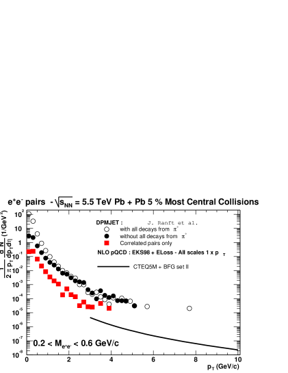
Figure 42: Lepton pair spectrum at $\eta=0$ in Pb+Pb collisions as a function of $p_{{}_{T}}$ for $\sqrt{s}=5.5$ TeV. The solid line indicates the prompt (signal) NLO QCD predictions while the squares and the points represent backgrounds of different origins calculated using Dpmjet. Thermal production will increase the signal (see sec. 7.3).

Using, from Appendix II, the luminosity factors for ALICE at $\sqrt{s}=$ 5.5 TeV, the rate of production of a prompt lepton pair in the mass range 0.2 GeV/c² $<M_{~{}e^{+}e^{-}}<$ 0.6 GeV/c² is estimated to be 6 pairs per second with $p_{{}_{T}}=3$ GeV/c and 0.1 pair per second with $p_{{}_{T}}=8$ GeV/c. The corresponding numbers in lead-lead collisions are 0.4 and 0.02 respectively. We should say at this point, that thermal production of dileptons (see next chapter) will increase the direct production of lepton pairs.

The production mechanism we just discussed suffers from a background with can be estimated using Dpmjet: indeed this code contains the Dalitz decays of resonances as well as the semi-leptonic decay processes of charmed and heavy flavor resonances. We show in Fig. 42 the prompt lepton pair spectrum for $0.2$ Gev/c${}^{2}<M_{~{}e^{+}e^{-}}<0.6$ Gev/c² (Eq. (17)) together with the background from lepton pairs originating from the same resonances (correlated pairs). One sees that, as expected, at high enough $p_{{}_{T}}$ the signal becomes comparable to the background.

Unfortunately, this estimate of the background is incomplete as one expects a huge contribution from uncorrelated pairs due to the large combinatoric factor when collecting pairs of leptons: in a typical Dpmjet event one expects about 180 $e^{-}$ and $e^{+}$ including $\pi^{~{}0}$ decays but only 17 $e^{-}$ and $e^{+}$ excluding $\pi^{~{}0}$’s. This is shown in the figure by the open dots (including $\pi^{~{}0}$ decays) and full dots (exluding $\pi^{~{}0}$ decays): obviously the situation is not as favorable since the background is now two orders of magnitude above the estimated signal! Note however the nice feature that the combinatoric background from $\pi^{~{}0}$’s disappears for $p_{{}_{T}}>2$ GeV/c. One way to tame the huge background may be to subtract from the data the spectrum of like charge pairs in the same kinematic range or pairs constructed from different events. Using low statistics runs of Dpmjet one finds that subtracting the like-charge pair spectrum from the unlike-charge pair spectrum one gets numbers which are very close to the correlated pair background whenever the transverse momentum of the pair is larger than 1.5 GeV/c [89]. The statistical fluctuations are large and clearly further studies are necessary to remove the uncorrelated background.

6 PHOTONS FROM THERMAL, EXPANDING FIREBALL

P. Aurenche, F. Gelis, G. Moore, H. Niemi, R. Rapp, K. Redlich, P.V. Ruuskanen, S.S. Räsänen, D.K. Srivastava

For the calculation of thermal photons — photons from secondary interactions among particles in the expanding fireball of matter produced in a heavy ion collision — the emission rates from hot matter and the space-time evolution of the matter are needed. The equilibrium emission rates in both QGP and the Hadron Resonance Gas (HRG) are reviewed below. The space-time evolution of expanding matter is described in terms of relativistic hydrodynamics with the assumption of longitudinal boost invariance.

There are uncertainties both in the emission rates and the description of the nuclear fireball. One such uncertainty affecting both the emission and the evolution of produced matter arises from the fact that the initially produced quark-gluon matter is not expected to be in chemical equilibrium. E.g., in the pQCD + saturation model [90] described below, most of produced partons are gluons. Assuming kinetic equilibrium and describing the deviation of number densities from equilibrium values in terms of fugacities, $\lambda_{i}$, we typically obtain $\lambda_{g}\sim 0.6...1$ and $\lambda_{q}\sim 0.2$ in the initially produced parton system. The quark fugacity is assumed to be the same at LHC energies as the antiquark fugacity. The effect of non-equilibrium values of fugacities on the photon emission rates is studied below. Using rate equations for reactions which change the parton numbers [91, 92], we will study in detail also the time evolution of fugacities.

The description of the space–time evolution of a fireball produced in a nucleus–nucleus collision must begin with characterization of the initial state of produced matter. Information on initial state is obtained from calculations of particle production from primary interactions in nuclear collisions. There are several model calculations, some more detailed than the others, of hadron spectra in heavy ion collisions at RHIC energies. We use these calculations or, when necessary, their extensions at the LHC energy as the first step in obtaining the initial state for the space-time evolution of produced matter. The most important quantities in determining the initial conditions are the total hadron multiplicity, $dN/dy$, which fixes the the total initial entropy and the production time scale, $\tau_{0}$. The initial densities are proportional to $dN/dy$ and $1/\tau_{0}$. The models for particle production differ also in the transverse dependence of nuclear densities.

After reviewing the emission rates both in the quark-gluon plasma and in the hot hadronic gas, we consider in Sec. 6.5 different models for particle production in order to establish a reasonable range of uncertainties in the initial state. The hydrodynamic evolution is dealt with in the following section, while the predictions for the rates of thermal pions and photons are discussed in Secs. 6.7 to 6.9. The last section is devoted to estimating the yield of small mass lepton pairs in the quark-gluon plasma.

6.1 Thermal photon emission rates

The rate of production, per unit time and volume, of a real photon of momentum ($E,\tenimbf p$) in a system in thermal equilibrium is calculated via the formula [93, 94]:

$$E{{dN}\over{dtd^{3}{\tenimbf x}d^{3}{\tenimbf p}}}=-{1\over{(2\pi)^{3}}}\;{1\over\exp(E/T)-1}\,{\rm Im}\,\Pi^{{}^{R}}{}_{\mu}{}^{\mu}(E,{\tenimbf p})\;,$$ (18)

where $\Pi^{{}^{R}}{}_{\mu}{}^{\mu}(E,{\tenimbf p})$ is the retarded photon polarization tensor. The pre-factor $1/(\exp(E/T)-1)$ provides the expected exponential damping when $E\gg T$.

A loop expansion of $\Pi^{{}^{R}}$ is constructed with effective propagators and vertices. For production of photons in the quark-gluon plasma the basic degrees of freedom are quarks and gluons and the corresponding physics will be discussed in the next two sections, while for production in hot hadronic matter the relevant degrees of freedom are mesons ($\pi$, $\rho$, $a_{1}$, $\cdots$) and baryons, and this will be the subject of Sec. 6.4.

6.2 Photon emission rates from the chemically equilibrated quark-gluon plasma

P. Aurenche, F. Gelis, G. Moore

The most complete calculations are those based on the improved perturbation theory of Braaten and Pisarski, i.e. on the Hard Thermal Loop (HTL) resummed effective theory [95, 96]. In the HTL approach, the quarks and the gluons acquire an effective mass of the order of $\sqrt{\alpha_{s}}T$, where $\sqrt{\alpha_{s}}$ is the strong coupling, due to their interactions in the plasma. Quark and gluon exchange mechanisms on a long distance (equivalently small momentum transfers) are also modified and they become effectively screened by mass effects of ${\cal O}(\sqrt{\alpha_{s}}T)$. Thus, thermal effects tend to regularize the infra-red behavior of the theory. Estimates of Eq. (18), in the HTL effective theory, based on 1-loop, 2-loop and multi-loop contributions have been performed: each case corresponds to different physical processes. We review them in turn.

6.2.1 Real photons

At one-loop order in the HTL theory, the production of a hard ($E\gg T$) real photon is given by the diagram in Fig. 43. One of the fermion leg in the loop may have a soft momentum flowing though it, the other one beeing necessarily hard. Following the HTL approach, thermal corrections are resummed on the soft line and an effective fermion propagator should be used. When taking the discontinuity of the diagram one of the cut fermions is necessarily space-like (denoted $Q$ in the figure) in the case of real photon production. Cutting through the effective quark propagator of momentum $Q$ exhibits Landau damping i.e., the exchange of a virtual quark in the scattering of quarks and gluons in the medium. In this way one obtains the processes contributing to photon production, namely Compton scattering and $q\bar{q}$ annihilation into a photon and a gluon. As a result of resummation, the potential singularity at 0 momentum transfer in the fermion propagator $Q$ is screened by an effective mass $m_{\rm q}$. Taking into account this thermal correction to the quark propagator, the imaginary part of the photon polarization tensor can be calculated [97, 98]. For hard photons, it reads:

$${\rm Im}\,\Pi^{{}^{R}}{}_{\mu}{}^{\mu}(E,{\tenimbf p})=4\pi{\frac{5\alpha\alpha_{s}}{9}}T^{2}\left[\ln\left(\frac{ET}{m_{\rm q}^{2}}\right)-\frac{1}{2}-\gamma_{{}_{E}}+\frac{7}{3}\ln(2)+\frac{\zeta^{\prime}(2)}{\zeta(2)}+{\cal O}({T\over E})\right]\;$$ (19)

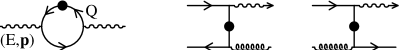
Figure 43: Left diagram: one-loop contribution to hard real photon production; right diagrams: examples of diagrams contributing to photon production, annihilation and Compton scattering. The symbol $\bullet$ on the quark propagator indicates that the effective propagator is used.

Note that the mass $m_{\rm q}$ is given by $m_{\rm q}^{2}=\pi\alpha_{s}C_{f}T^{2}$ with $C_{f}\equiv(N_{c}^{2}-1)/2N_{c}$. The numerical factor $5/9$ is the sum of the quark electric charges squared for $2$ flavors (u and d); for $3$ flavors (u, d and s), this factor should be replaced by $6/9$. It is clear from the expression above that the quark thermal mass acts as the cut-off of a logarithmic collinear singularity.

For some time this was thought to be the final answer for the photon rates at ${\cal O}(\alpha_{s})$. It then became clear that some formally higher order processes (see Fig. 44) are in fact strongly enhanced by collinear singularities. The corresponding processes are bremsstrahlung emission and off-shell annihilation. A common property of these two diagrams is that they have an off-shell quark next to the vertex where the photon is emitted, and the virtuality of this quark becomes very

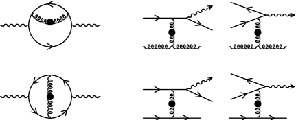
Figure 44: Left most diagrams: two-loop contributions to hard real photon production; right diagrams: bremsstrahlung and off-shell annihilation processes. The symbol $\bullet$ on the gluon propagator indicates that the effective propagator is used.

small if the photon is emitted forward. Again, the quark thermal mass $m_{\rm q}$ prevents these diagrams from being truly singular. However, contrary to the one loop diagrams, the singularity is linear instead of logarithmic, and it brings a factor $T~{}^{2}/m_{\rm q}^{2}$. Combined with $\alpha_{s}^{2}$ from the vertices, these diagrams turn out to be also of order ${\cal O}(\alpha_{s})$ [99, 100, 101, 102]. For 3 colors and 2 light quark flavors, the ${\cal O}(\alpha_{s})$ contribution of these two diagrams is exactly:

$${\rm Im}\,\Pi^{{}^{R}}{}_{\mu}{}^{\mu}(E,{\tenimbf p})=\frac{32}{3\pi}\,\frac{5\alpha\alpha_{s}}{9}\left[\pi^{2}\frac{T^{3}}{E}+ET\right]\;.$$ (20)

In this formula, the term in $1/E$ comes from the bremsstrahlung diagram and dominates for soft photons, while the term linear in $E$ comes from off-shell annihilation which therefore dominates for very hard photons ($E\gg T$).

Given the enhancement in the diagrams of Fig. 44, one may wonder if higher order diagrams also contribute to the same ${\cal O}(\alpha_{s})$ order. To discuss the issue in physical terms, it is convenient to define the concept of photon formation time. Consider a virtual quark of momentum $R\equiv P+Q$ which splits into an on-shell quark of momentum $Q$ and a photon of momentum $P$ (see the processes in Fig. 44). The photon formation time can be identified with the lifetime of the virtual quark, which is itself related to its virtuality by the uncertainty principle. A simple calculation gives:

$$t_{{}_{F}}^{-1}\sim{\delta E}=r_{0}-\sqrt{{\boldsymbol{r}}^{2}+m_{\rm q}^{2}}\approx\frac{E}{2q_{0}r_{0}}\left[{\boldsymbol{q}}_{\perp}^{2}+{m_{\rm q}^{2}}\right]\;,$$ (21)

where the 3-momentum of the photon defines the longitudinal axis. The collinear enhancement in the diagrams of Fig. 44, due to the small virtuality of the quark that emits the photon, can be rephrased by saying that it is due to a large photon formation time, of ${\cal O}(1/\alpha_{s}T)$. If the formation time is large, the quark can rescatter in the medium, while emitting the photon, as it is shown in Fig. 45. This can be partially taken into account by introducing a collisional width $\Gamma\sim\alpha_{s}T\ln(1/\alpha_{s})$ on the quarks in the calculation of the diagrams of Fig. 44 [103]. A large sensitivity to this parameter was found at leading order, thereby indicating that an infinite series of diagrams must be resummed in order to fully determine the ${\cal O}(\alpha_{s})$ photon rate. This phenomenon is nothing but a manifestation of the Landau Pomeranchuk Migdal (LPM) effect [104, 105, 106].

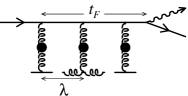
Figure 45: A ladder correction to bremsstrahlung.

A considerable progress was made recently in [107]: it was shown that there are infrared cancellations between diagrams of different topologies, and that these cancellations remove any sensitivity to the magnetic scale. Physically, this cancellation can be interpreted as the fact that ultrasoft scatterings are not efficient in order to induce the production of a photon. As a consequence, only the ladder family of diagrams needs to be resummed in order to obtain the complete leading ${\cal O}(\alpha{}_{s})$ photon rate. The resummation of this series of diagram can then be performed in two steps summarized in Fig. 46.

Figure 46: Resummation of ladder diagrams.

The first one is a Dyson equation for the photon polarization tensor, whose explicit form is [107, 108, 109]:

$${\rm Im}\,\Pi^{{}^{R}}{}_{\mu}{}^{\mu}(E,{\tenimbf p})\approx{\alpha N_{c}}\int_{-\infty}^{+\infty}\!\!dq_{0}\,[n_{q}(r_{0})-n_{q}(q_{0})]\;\frac{q_{0}^{2}+r_{0}^{2}}{(q_{0}r_{0})^{2}}\,{\rm Re}\int\frac{d^{2}{\boldsymbol{q}}_{\perp}}{(2\pi)^{2}}\;{\boldsymbol{q}}_{\perp}\cdot{\boldsymbol{f}}({\boldsymbol{q}}_{\perp})\;,$$ (22)

with $r_{0}\equiv E+q_{0}$, $n_{q}(r_{0})\equiv 1/(\exp(r_{0}/T)+1)$ the Fermi-Dirac statistical weight, and where the dimensionless function ${\boldsymbol{f}}({\boldsymbol{q}}_{\perp})$ denotes the resummed vertex between the quark line and the transverse modes of the photon (this is represented by the shaded vertex in the above pictures). In the Dyson equation, this function is dotted into a bare vertex, which is proportional to ${\boldsymbol{q}}_{\perp}$ (the photon has a transverse polarization and therefore the coupling vanishes for a collinear emission by a quark). The second equation, that determines the value of ${\boldsymbol{f}}({\boldsymbol{q}}_{\perp})$, is a Bethe-Salpeter equation that resums all the ladder corrections [107, 108, 109]:

$$\frac{i}{t_{{}_{F}}}{\boldsymbol{f}}({\boldsymbol{q}}_{\perp})=2{\boldsymbol{q}}_{\perp}+4\pi\alpha_{s}C_{f}T\!\!\int\frac{d^{2}{\boldsymbol{l}}_{\perp}}{(2\pi)^{2}}\,{\cal C}({\boldsymbol{l}}_{\perp})\,[{\boldsymbol{f}}({\boldsymbol{q}}_{\perp}+{\boldsymbol{l}}_{\perp})-{\boldsymbol{f}}({\boldsymbol{q}}_{\perp})]\;,$$ (23)

where $t_{{}_{F}}$ is the time defined in Eq. (21) and where the collision kernel has the following expression: ${\cal C}({\boldsymbol{l}}_{\perp})={m^{2}_{\rm debye}}/{{\boldsymbol{l}}_{\perp}^{\ 2}}({{\boldsymbol{l}}_{\perp}^{\ 2}+{m^{2}_{\rm debye}}})$ [102]. Note that in the Dyson equation, the quark propagators are dressed (by resumming self-energy corrections which is akin to introducing the collisional width or damping rate) to match the resummation performed for the vertex, so that gauge invariance is preserved. It is this dressing on the quark propagators which is responsible for the term $-{\boldsymbol{f}}({\boldsymbol{q}}_{\perp})$ under the integral in Eq. (23). From this integral equation, it is easy to see that each extra rung in the ladder contributes a correction of order $\alpha_{s}Tq_{0}r_{0}/Em_{\rm q}^{2}$, in which the $\alpha_{s}$ drops out. Therefore, all these corrections contribute to ${\cal O}(\alpha_{s})$ to the photon rate. Note again that the only parameters of the QGP that enter this equation are the quark thermal mass $m_{\rm q}$ and the Debye screening mass, $m_{\rm debye}$. This integral equation was solved numerically in [108], and the results are displayed in Fig. 47.

Figure 47: ${\cal O}(\alpha_{s})$ contributions to the photon production rate in a QGP. The parameters used in this plot are $\alpha_{s}=0.3$, 3 colors, 2 flavors and $T=1$ GeV.

In this plot, ‘LPM’ denotes the contribution of all the multiple scattering diagrams, while ‘$2\to 2$’ denotes the processes of figure 43. The single scattering diagrams (Fig. 44) are also given so that one can appreciate the suppression due to the LPM effect.

6.2.2 Small mass lepton pairs

For the reasons given in Sec. 5.6, it is also interesting to consider the production of a small mass leptons pair at hard momentum. The calculation parallels that described above with added technical complications due to the mass of the virtual photon (lepton pair). The relation between the rate of production of a pair of mass $M$ at 4-momentum $(E,{\tenimbf p})$ and the virtual photon polarization tensor is

$${{dN}\over{dtd^{3}{\tenimbf x}dEd^{3}{\tenimbf p}}}=-{1\over{12\pi^{4}}}\;{\alpha\over M^{2}}\;{1\over\exp(E/T)-1}\,{\rm Im}\,\Pi^{{}^{R}}{}_{\mu}{}^{\mu}(E,{\tenimbf p})\;.$$ (24)

Neglecting the mass of the pair compared to its energy, the imaginary part of the photon polarization tensor at one-loop is still given by Eqs. (19) but the collinear cut-off (quark thermal mass) in the logarithmic term now involves the photon mass [110, 111]. The two-loop [112] and the multi-loop [113] calculations have been carried out. In the latter case, it is convenient to separate the contributions of the transverse and longitudinal polarizations. For the transverse case, one obtains again Eqs. (23), (22) while a related integral equation has been derived and solved for the case of the longitudinal polarization [113].

6.3 Hard photon production from hot out-of-chemical equilibrium QGP

F. Gelis, K. Redlich

As a first step we consider only the basic reactions for photon production due to Compton scattering and annihilation of quarks (see Fig. 43). We assume that off-equilibrium effects on the momentum of QGP constituents can be parameterized by a modification of their distributions. A HTL-resummation is also supposed to be valid to screen soft and collinear (mass) singularities.

To account for non-equilibrium effects in partonic medium we follow the approximations described in detail in [114, 115, 116]. It amounts simply to replace the thermal particle energy distribution $n(k{~{}}_{0})$ by their non-equilibrium counterparts, i.e. in general by Wigner distributions $n(k{~{}}_{0},X)$. In terms of the cumulant expansion of the initial density operator, this amounts to approximate the initial correlations by the second cumulant only, i.e. to neglect all non-gaussian correlations. As a further approximation, we ignore for the time being the possible dependence on the center-of-mass coordinate $X$, essentially assuming a homogeneous and isotropic medium. Practically, we take the following distributions for quarks and gluons:

$$n_{q}(k_{0})\equiv\left\{\begin{array}[]{c}n_{q}(|k_{0}|)\\ 1-n_{q}(|k_{0}|))\end{array}\right.\quad\quad n_{g}(k_{0})\equiv\left\{\begin{array}[]{c}n_{g}(|k_{0}|)\\ -(1+n_{g}(|k_{0}|))\end{array}\right.\quad\mbox{for}\quad\begin{array}[]{c}k_{0}>0\\ k_{0}<0\end{array}$$ (25)

with the Jüttner parameterizations

$$n_{g(q)}(|k_{0}|)\equiv\frac{\lambda}{e^{|k_{0}|/T}\mp\lambda}\;,$$ (26)

expressed by introducing the fugacity parameter $\lambda$ [118], which is assumed to be energy independent. Obviously $\lambda\not=1$ in the case of chemical non-equilibrium.

Neglecting the slow macroscopic scale $X$ compared to the fast microscopic scale, the structure of the resulting perturbation theory is very similar to the equilibrium Closed Time Path formalism. For instance, the $21$ components of the non-equilibrium bare propagators for bosonic and fermionic fields,

$$iD_{21}(P)=2\pi\varepsilon(p_{0})\delta(P^{2})(1+n_{g}(p_{0}))\;,\quad iS_{21}(P)=2\pi\delta(P^{2})\raise 0.6458pt\hbox{$/$}\kern-5.29999pt\hbox{$P$}\varepsilon(p_{0})(1-n_{q}(p_{0}))\;,$$ (27)

have formally the same structure as the corresponding ones in equilibrium, but depend now on the modified distribution functions (Eq. 25). However, for a dressed propagator the above is not in general valid, as the appearance of some additional out-of-equilibrium terms is to be expected [110, 119, 120]. Therefore, in order to calculate a physical rate with this formalism, one needs to account not only for the modifications of the particle momentum distributions but also for modifications of their propagators.

The rate of real photon emission, already given in Eq. (18) in terms of the retarded photon polarization tensor, can also be written in terms of its component $\Pi{~{}}_{12}$ in the Closed Time Path formalism:

$$E\frac{dN}{dtd^{3}{\boldsymbol{x}}d^{3}{\boldsymbol{p}}}=\frac{i}{2(2\pi)^{3}}{\Pi_{12}}{}_{\mu}^{\mu}(E,{\boldsymbol{p}}),\;.$$ (28)

As in the equilibrium case the simplest diagrams, in the loop expansion of $\Pi{~{}}_{12}$, correspond to photon production by annihilation and Compton processes $q+\bar{q}\to g+\gamma,\;q(\bar{q})+g\to q(\bar{q})+\gamma\;,$ as shown in Fig. 43. In the off-equilibrium situation one needs first to determine the appropriate generalization of the effective quark propagator. In the un-resummed theory it is known that ill-defined terms of the form $\delta(Q^{2})/Q^{2}$ are generated. However, in the resummed approach one can show that quark propagator can be approximated by a form similar to the equilibrium one [121, 122]:

$$S_{12}^{{}^{HTL}}(Q)=-n_{q}(q_{0})\;{\rm Re}\,\left[\frac{i}{\raise 0.6458pt\hbox{$/$}\kern-5.29999pt\hbox{$Q$}-\Sigma^{{}^{HTL}}_{{}_{R}}(q)+i\varepsilon q_{0}}\right]\;,$$ (29)

where $\Sigma^{{}^{HTL}}$ is the quark HTL self-energy, evaluated with non-equilibrium distribution functions. The only non-equilibrium effect on this HTL self-energy amounts to a modification of the quark thermal mass $m_{q}$ (the prefactor in $\Sigma^{{}^{HTL}}$):

$$m_{\rm q}^{2} = \frac{g^{2}}{\pi^{2}}C_{f}\int_{0}^{\infty}EdE[n_{g}(E)+n_{q}(E)]=\pi\alpha_{s}C_{f}T^{2}{2\over 3}\left(\lambda_{g}+\frac{\lambda_{q}}{2}\right)\;.$$ (30)

which reduces to the expression given in the previous section in the equilibrium case ($\lambda{}_{g}=\lambda{}_{q}=1$).

The hard photon production rate from a system away from equilibrium can then be calculated using well established methods in equilibrium field theory. The final result in the leading order in $\alpha{}_{s}$ is [122] (cf Eq. 19 for the equilibrium result):

$$E\frac{dN}{dtd^{3}{\boldsymbol{x}}d^{3}{\boldsymbol{p}}}=e_{q}^{2}\frac{\alpha\alpha_{s}}{2\pi^{2}}\lambda_{q}T^{2}e^{-E/T}\left[\frac{2}{3}(\lambda_{g}+\frac{\lambda_{q}}{2})\ln\left(\frac{ET}{m_{\rm q}^{2}(\lambda_{q},\lambda_{g})}\right)+\frac{4}{\pi^{2}}C(E,T,\lambda_{q},\lambda_{g})\right]\;,$$ (31)

with

$$C(E,T,\lambda_{q},\lambda_{g}) \equiv \lambda_{q}\left[-1+(1-\frac{\pi^{2}}{6})\gamma+(1-\frac{\pi^{2}}{12})\ln\frac{E}{T}+\zeta_{-}\right]$$ (32)

$$+\lambda_{q}\lambda_{g}\left[\frac{1}{2}-\frac{\pi^{2}}{8}+(\frac{\pi^{2}}{4}-2)(\gamma+\ln\frac{E}{T})+\frac{3}{2}\zeta^{\prime}(2)+\frac{\pi^{2}}{12}\ln 2+(\zeta_{+}-\zeta_{-})\right]$$

$$+\lambda_{g}\left[\frac{1}{2}+(1-\frac{\pi^{2}}{3})\gamma+(1-\frac{\pi^{2}}{6})\ln\frac{E}{T}-\zeta_{+}\right]\;,$$

where $\gamma$ is Euler’s constant, $\zeta^{\prime}$ the derivative of Riemann’s function and where we have defined:

$$\zeta_{+}\equiv\sum_{n=2}^{\infty}\frac{1}{n^{2}}\ln(n-1)\simeq 0.67,\qquad\zeta_{-}\equiv\sum_{n=2}^{\infty}\frac{(-)^{n}}{n^{2}}\ln(n-1)\simeq-0.04\;.$$ (33)

The above result shows that, as in the equilibrium medium, the generalized thermal mass provides a self consistent cut-off for the logarithmic singularity. The dynamical screening of the mass singularity seen in Eq. (31) (here given for the distributions Eq. (26)) actually does not depend on the explicit form of the non-equilibrium quark and gluon distribution functions. Changing the parameterization of these functions enters only through the redefinition of the mass parameter in Eq. (31) and the constant $C$ in Eq. (32), keeping at the same time the functional form of the rate unchanged. For $\lambda{}_{q}=\lambda{}_{g}=1$ Eqs. (31), (32) reproduce the well known one-loop results of the previous section.

The out-of-equilibrium approach discussed above for the case of Compton and $q\bar{q}$ annihilation processes can also be extended to the more complicated processes of Fig. 44. The main effect of the fugacities comes from the fact that the number of emitters is reduced. To take this into account, one just need to rewrite the statistical functions in Eqs. (18) and (22) as:

$$\frac{1}{\exp(E/T)-1}[n_{q}(p_{0}+E)-n_{q}(p_{0})]=-n_{q}(p_{0}+E)n_{q}(-p_{0})\;.$$ (34)

Since the equilibrium quark distribution function satisfies $n_{q}(-x)=1-n_{q}(x)$, one sees readily that the right hand side of the previous formula gives the combination of distribution functions one expects from kinetic theory in each of the kinematical domains: for $p_{0}>0$ (bremsstrahlung of a quark) we get $n_{q}(p_{0}+E)(1-n_{q}(p_{0}))$, for $-E<p_{0}<0$ (quark-antiquark annihilation with a scattering) we get $n_{q}(p_{0}+E)n_{q}(|p_{0}|)$, and for $p_{0}<-E$ (bremsstrahlung of an antiquark) we get $n_{q}(|p_{0}|)(1-n_{q}(|p_{0}+E|))$. Given its interpretation in terms of kinetic theory, the right hand side of Eq. (34) can be generalized to out of chemical equilibrium situations by simply replacing the Fermi distribution by the form of Eq. (26). For this to make sense, the out-of-equilibrium distribution at negative arguments must be defined in such a way that $n_{q}(-x)=1-n_{q}(x)$ holds, which is indeed the case (see Eqs. (25)).

The other places where the fugacities enter in the calculation of the multiple scattering diagrams is via the quark thermal mass $m_{\rm q}^{2}$ and via the Debye mass $m_{\rm debye}^{2}$. We recall here the expression for these masses:

$$m_{\rm q}^{2}=\frac{g^{2}C_{{}_{F}}T^{2}}{6}(\lambda_{g}+\frac{\lambda_{q}}{2})\;,$$ (35)

$$m_{\rm debye}^{2}=\frac{g^{2}T^{2}}{3}(N_{c}\lambda_{g}+N_{f}\frac{\lambda_{q}}{2})\;.$$ (36)

It is interesting to remark that using fugacities $\lambda_{q},\ \lambda_{g}<1$ will obviously reduce the photon rate, because the number of emitters is reduced, however, since the thermal quark mass is also decreased, the collinear enhancement at work in bremsstrahlung and off-shell annihilation processes is increased. The two effects partly compensate [123]

6.4 Thermal photon production from hadronic matter

R. Rapp

The objective in the following is to assess the emission rate of photons in a hot hadron gas as expected to be formed under conditions characteristic for LHC heavy-ion collisions. The rate is calculated acording to Eq. (18).

6.4.1 $\pi\rho a_{1}$ gas and form factors

Early calculations [97] of photon radiation from hadronic matter were guided by the analogue to lowest-order pQCD processes in a QGP, i.e., Compton and annihilation graphs involving the most abundant constituents in a meson gas. These were $\pi\pi\to\rho\gamma$, $\pi\rho\to\pi\gamma$ as well as $\rho\to\pi\pi\gamma$ (and $\omega\to\pi\gamma$), which are based on the $\pi\pi\rho$-vertex with a coupling constant determined from the free $\rho$ ($\omega$) decay. At photon energies in excess of $E\simeq$ 1 GeV, $t$-channel pion exchange in the second reaction completely dominates the rate. Shortly thereafter [124], the $a_{1}$ $s$-channel pole graph was recognized as a potentially relevant contribution, due its large coupling to $\pi\rho$ states. At sufficiently high energies, $s$-channel resonance graphs are, however, suppressed due to $1/(s-m_{R}^{2})$ powers in the intermediate propagators ($m_{R}$: resonance mass), rendering $a_{1}$ $t$-channel graphs increasingly important. A systematic evaluation of photon production from a $\pi\rho a_{1}$ gas, based on the Massive Yang-Mills (MYM) Lagrangian approach, has been performed in ref. [125]. Here, chiral symmetry provides relations between couplings, leaving 4 free parameters (including non-minimal coupling terms) allowing for a reasonable phenomenology for the free $\pi\rho a_{1}$ system with electromagnetic decays. Two different sets implying different off-shell behaviors lead to total rates that differ by no more than 50%. The dominant contribution to the rate at photon energies beyond $\sim$ 0.5 GeV was confirmed to be due to $t$-channel ($\pi$ and $a_{1}$) exchanges in the $\pi\rho\to\pi\gamma$ reaction [125]. A convenient parametrization of the pertinent results, which will be used below, has been provided in ref. [126].

Figure 48: Thermal photon production rates from the $\pi\rho\to\pi\gamma$ reaction within $SU(2)$ chiral lagrangians including vector mesons using the Massive Yang-Mills [125] (dotted line) and Hidden-Local Symmetry [127] (full line). The dashed line is from the earlier work of ref. [97] which does not include $a_{1}$ degrees of freedom.

An important element in applying effective hadronic models at moderate and high momentum transfers is the use of vertex form factors to simulate finite hadronic-size effects, which are not accounted for in the $\pi\rho a_{1}$ calcuations of Ref. [125]. For similar reactions their effect has been studied in Ref. [97] and found to give a typical net suppression over the bare graphs by a significant factor $\sim$3 at photon energies $E\simeq 2.5$ GeV. We perform a rough estimate of their effect in the present context as follows. Consider pion-exchange assuming a standard dipole form factor,

$$F(t)=\left(\frac{2\Lambda^{2}}{2\Lambda^{2}-t}\right)^{2}\ ;$$ (37)

the average four-momentum transfer in $t$-channel pion exchange can be approximated according to

$$\frac{1}{(m_{\pi}^{2}-\bar{t})^{2}}=\frac{1}{4E^{2}}\int\limits_{0}^{4E^{2}}dt\ \frac{1}{(m_{\pi}^{2}-t)^{2}}\simeq\frac{1}{m_{\pi}^{2}4E^{2}}\ ,$$ (38)

that is

$$-\bar{t}\simeq 2\ E\ m_{\pi}$$ (39)

at sufficiently large $E>m_{\pi}$. Upon multiplying the rate parametrizations of the $\pi\rho a_{1}$ gas [126] (dotted line in Fig. 49) by $F(\bar{t})^{2}$ (with $\Lambda=1$ GeV [128]) we obtain the dashed curve in Fig. 49.

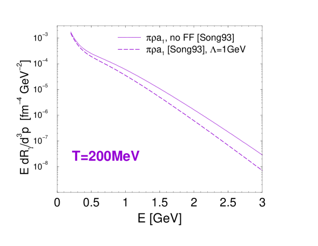
Figure 49: Effect of hadronic form factors on the photon production rates from a $\pi\rho a_{1}$ gas in the MYM approach of ref. [125].

The reduction of the rate in the 2-3 GeV region amounts to a factor of 3-4, quite in line with the exemplary microscopic calculation of Ref. [97].

We believe that the calculation including formfactors should provide a reasonable baseline for the $SU(2)$ case.

6.4.2 Additional mesonic sources

An obvious contribution to photon production not accounted for in the previous section stems from radiative decays of heavier mesonic resonances which can not be easily treated in a chiral framework. In the many-body approach of Refs. [128, 129] the electromagnetic correlator has been evaluated including all mesonic resonances up to about 1.4 GeV in mass which exhibit significant coupling to final states including rho-mesons (and thus, employing VDM, photons), These are $\omega(782)$, $h_{1}(1170)$, $f_{1}(1285)$, $\pi(1300)$, $a_{(}1320)$, $K^{*}(892)$ and $K_{1}(1270)$. Pertinent photon rates are displayed in Fig. 50. In particular, the $\omega\to\pi\gamma$ decay generates a large low-energy strength, consistent with the early results of Ref. [97]. Note that all hadronic vertices carry (dipole) formfactors with typical cutoff parameters of around 1 GeV, as extracted from an optimal fit to measured hadronic and radiative branching ratios within VDM (see Ref. [128] for details). Contributions from still higher-mass mesonic resonances (such as $\omega(1420)$ and $\omega(1650)$) have recently been computed [130] and turned out to be negligible.

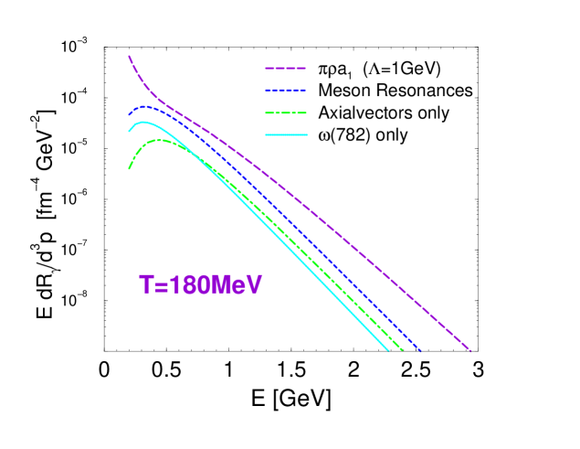
Figure 50: Various sources of thermal photon production from a hot meson gas.

Another significant photon source can be expected from additional $t$-channel exchanges, in particular $\omega(782)$ exchange in $\pi\rho\to\pi\gamma$, and pion-exchange in $\pi K\to\gamma K^{*}(892)$, $\pi K^{*}(892)\to K\gamma$. Results for the former, which do not seem to be available in the literature yet, have been obtained recently [130], indicating an emission strength that is small at low energies but exceeds the in-medium many-body results of ref. [128] beyond $E\simeq 1.5-2$ GeV. For the kaon-induced processes, one can use $SU(3)$ symmetry to estimate the relevant couplings from the analogue $SU(2)$ processes, i.e., $\pi\pi\to\gamma\rho$, $\pi\rho\to\rho\gamma$, and account for the smaller kaon ($K^{*}$) densities ($n_{K+\bar{K}}/n_{\pi}\sim$ 40% at maximal SPS energies and beyond). One finds that the strange analogues make up less than 10% in the former case, and about 20% in the latter.

6.4.3 Baryonic sources

Finally we have to address the role of baryons. Naively, one might not expect significant contributions at collider energies where the net baryon densities are small. However, since the photon is a $CP$ eigenstate, the relevant quantity for its production is the sum of baryon and anti-baryon densities, which is not small at temperatures close to $T_{c}$ even in a net baryon-free environment [131]. Moreover, since the corresponding anti-/baryon content survives the subsequent hadronic evolution in a heavy-ion collision [132, 133], their effects on photon and dilepton observables remain appreciable also in the later stages.

Much like in the mesonic case, baryon-resonance decays ought to be rather suppressed at energies beyond 1 GeV. No explicit computation of $t$-channel exchanges has been reported so far. However, within the chiral reduction formalism, contributions from nucleons have been assessed in ref. [134]. Within a hadronic many-body framework [135, 129, 128], primarily constructed for low-mass dilepton applications, the e.m. correlator has been evaluated incorporating a rather extensive set of baryonic processes. These results can be straightforwardly extrapolated to the photon point, and the corresponding rate is shown by the solid line in Fig. 51.

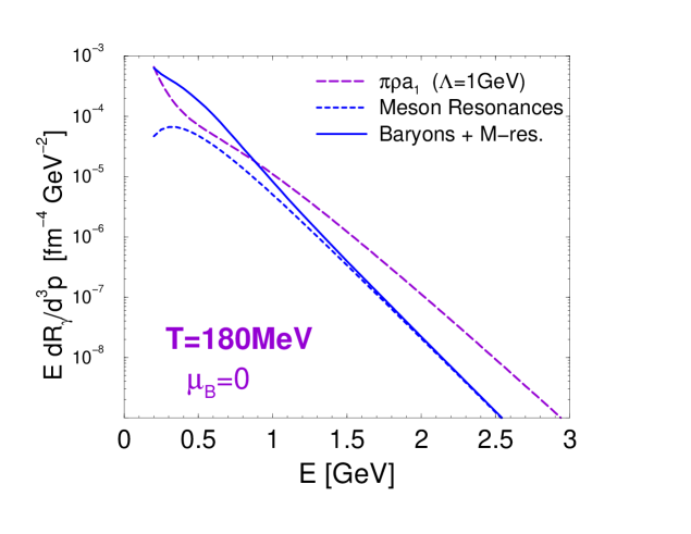
Figure 51: Thermal photon production rate (under conditions resembling LHC energies) for a $\pi\rho a_{1}$ gas [125] including formfactors (long-dashed lines), and within the many-body spectral function approach of ref. [129] (full line). The total emissivity corresponds to the sum of the two rates; $\omega$ $t$-channel and strange-meson processes, not included in the figure, are expected to induce an additional increase of about 30-40% at energies above 1.5 GeV.

More specifically, both the mesonic resonance contributions as discussed above (short-dashed line), as well as baryonic resonance decays (most notably $\Delta(1232)$, $N(1520)$) and pion-exchange processes involving nucleons and deltas, are included coherently. The baryon-induced emission can be considered as rather reliable for baryon densities up to at least normal nuclear matter density, $\rho_{0}=0.16$ fm^-3, being constrained by photoabsorption spectra on nucleons and nuclei [136] (at zero temperature). At comparable baryonic densities this approach yields about a factor of two more photons than what has been found in the chiral reduction approach [134] when coupling on-shell pions and nucleons (see Ref. [137] for an update including $\Delta(1232)$ and $N(1520)$ resonances).

Under conditions relevant for LHC energies (as chosen in the figure), processes involving (anti-) baryons are the prevailing source of thermal photons at energies $E<1$ GeV (similar to what has been found for low-mass dileptons [131]). Beyond, the $t$-channel processes within the light meson gas sector take over, dominating the rate at higher energies.

It is thus suggestive to regard the combination of the $\pi\rho a_{1}$ emission rate (including form factor effects), supplemented with $\omega$ $t$-channel and kaon-induced proceses, with the hadronic many-body results ($a_{1}$ contribution removed) as a semi-realistic approximation to the full hadron gas emissivity.

6.5 Particle production from primary interactions in nuclear collisions

K.J. Eskola, J. Ranft, P.V. Ruuskanen

Results from model calculations of initial particle production are the average numbers, transverse energies and momentum spectra of produced gluons and quarks. How to obtain from the momentum space densities the space-time densities needed for the hydrodynamic calculation is explained in detail in Sec. 6.6.2 using the pQCD + saturation calculation of (mini)jet production [90] as an example.

The essential quantities in determining the initial state for the hydrodynamic expansion are (i) the total multiplicity $dN/dy$, (ii) the initial time scale $\tau_{0}$ and (iii) the shape of the transverse distribution. Production models differ on all these and our aim in discussing model calculations is to estimate what are the present uncertainties in these quantities. We can then vary the initial conditions accordingly to explore the range of uncertainty in predicting the thermal photon spectrum in the nucleus–nucleus collision at LHC.

In this subsection, we consider different approaches to primary production: (i) pQCD + final state saturation (minijet) [90] and (ii) initial state saturation, the colour glass condensate model [138], which both describe the produced matter as a parton system. We also discuss the string based model Dpmjet, of Ranft and collaborators, already presented in Sec. 5.2 (see refs. [68, 69, 74, 75]).

6.5.1 Perturbative QCD + saturation model

In the pQCD + saturation model [90] one assumes that at collider energies the production of final state particles is dominated by collinearly factorized parton (minijet) production above a momentum scale, ${p_{\rm sat}}\gg{\Lambda_{\rm QCD}}$, determined from an assumption that saturation reduces parton production below this scale and gives only a minor contribution which can be effectively included in the contribution from partons above ${p_{\rm sat}}$.

The numerical minijet calculation [139, 140] gives the cross sections $d\sigma_{i}(\Delta y)/dp_{{}_{T}}$ in the rapidity interval $\Delta y$ for parton species $i=g,q$ and $\bar{q}$. For $\Delta y\raise 1.29167pt\hbox{$<$\kern-7.5pt\raise-4.73611pt\hbox{$\sim$}}1$ (around $y=0$), the cross section is proportional to $\Delta y$ and the differential cross section can be defined as

$$\frac{d\sigma}{dydp_{{}_{T}}^{2}}=\frac{1}{\Delta y}\frac{d\sigma(\Delta y)}{dp_{{}_{T}}^{2}}=\frac{1}{\Delta y}\int_{\Delta y}dy_{1}\int dy_{2}\sum_{ijkl}f_{i/A}(x_{1},Q^{2})f_{j/A}(x_{2},Q^{2})\frac{d\hat{\sigma}}{d\hat{t}}^{ij\rightarrow kl}$$ (40)

with nuclear parton distributions $f_{i/A}$, momentum fractions $x_{1,2}$, scale $Q=p_{{}_{T}}$ and the partonic cross sections $d\hat{\sigma}$. The basic quantities for the calculation of initial densities in nucleus–nucleus collisions (cf. Sec. 6.6.2) are the integrated and $p_{{}_{T}}$-weighted cross sections

$$\int_{p_{0}}^{\infty}dp_{{}_{T}}\frac{d\sigma_{i}}{dydp_{{}_{T}}} = \frac{1}{\Delta y}\int_{p_{0}}^{\infty}dp_{{}_{T}}\frac{d\sigma_{i}(\Delta y)}{dp_{{}_{T}}}=\frac{1}{\Delta y}\sigma_{i}(p_{0},\Delta y)=\frac{d\sigma_{i}(p_{0})}{dy}\,,$$ (41)

$$\int_{p_{0}}^{\infty}dp_{{}_{T}}p_{{}_{T}}\frac{d\sigma_{i}}{dydp_{{}_{T}}} = \frac{1}{\Delta y}\int_{p_{0}}^{\infty}dp_{{}_{T}}p_{{}_{T}}\frac{d\sigma_{i}(\Delta y)}{dp_{{}_{T}}}=\frac{1}{\Delta y}\sigma_{i}\langle E_{{}_{T}}\rangle(p_{0},\Delta y)=\frac{d\sigma_{i}\langle E_{{}_{T}}\rangle(p_{0})}{dy}\,.$$ (42)

When multiplied with the nuclear overlap function $T_{AA}$ (see Eq. 102 and appendix 1 for further details), $\sigma_{i}(p_{0},\Delta y)$ gives the average number and $\sigma_{i}\langle E_{{}_{T}}\rangle(p_{0},\Delta y)$ the average transverse energy of partons $i$ in a rapidity interval $\Delta y$ with transverse momenta above $p_{0}$. The number of partons is well-defined only in the leading order, at higher orders it is not an infrared safe quantity. The transverse energy, however, is well-defined, and it has been computed to next-to-leading order in [141, 142]. The factor $K=1.6$ from such a computation for the LHC energy is used to estimate the effect of the NLO contributions both to the number and the transverse energy of produced partons. In what follows, the number of partons is used in estimating the chemical composition of produced partons but the initial energy is determined from the produced total transverse energy alone. Nuclear shadowing, as given by the EKS parametrization [39, 40], is included in the calculation of these cross sections.

To close the calculation, the cut-off momentum $p_{0}$ for central $AA$ collisions is fixed as the saturation scale, ${p_{\rm sat}}$, from a geometric condition

$$T_{AA}(0)\frac{\sigma({p_{\rm sat}},\Delta y)}{\Delta y}\frac{\pi}{{p_{\rm sat}}^{2}}=\pi R_{A}^{2}\,,$$ (43)

which is solved numerically. We fix $\Delta y=1$. The condition above can be interpreted as giving the parton density at which the produced partons begin to overlap leading to fusions which suppress the further production of softer partons. The condition can also be interpreted as the beginning of overlap of primary interaction volumes that can also be expected to suppress the further yield of partons.

Once the saturation momentum ${p_{\rm sat}}$ has been obtained from the condition above, the initial production cross sections $\sigma_{i}({p_{\rm sat}},\Delta y)$ and $\sigma_{i}\langle E_{{}_{T}}\rangle({p_{\rm sat}},\Delta y)$ can be calculated. Although the pQCD+saturation model is an effective (non-microscopic) approach to describe the bulk of the initial parton production at central rapidities of nearly central $AA$ collisions, it provides enough information to fully determine the initial state for the hydrodynamic evolution if the initial time is given. With the hydrodynamic evolution [143] it has correctly predicted the multiplicities in central Au+Au collisions at RHIC energies $\sqrt{s}=56$, 130 and 200 GeV [143, 144], and also given a successful description of the transverse momentum spectra of pions, kaons and (anti)protons [145].

Using the notation $\sigma(1)=d\sigma/dy$, the integrated partonic cross sections at $\sqrt{s}=5.5$ TeV, the energy of lead–lead collisions at LHC, are $\sigma_{g}(1)=135$ mb, $\sigma_{q}(1)=6.46$ mb, $\sigma_{\bar{q}}(1)=6.14$ mb, while the $p_{{}_{T}}$-weighted cross section becomes $\sigma\langle E_{{}_{T}}\rangle(1)=468$ mb GeV. The saturation scale is ${p_{\rm sat}}=2.03$ GeV. Below in Sec. 6.6.2, initial energy density and initial values of gluon and (anti)quark fugacities are constructed from these cross sections.

6.5.2 Initial state parton saturation and color glass condensate

A much discussed theoretical approach to particle production in heavy-ion collisions at collider energies has been based on the assumption that the initial state parton densities saturate and non-linear dynamics becomes dominant [138]. This means that the parton (gluon) densities in a nucleus (or in a proton) at small $x$ are so high, that gluons interact coherently. From the point of view of the color fields, the high density or large occupation numbers of the field quanta can be described as the formation of a ”color glass condensate” which can be treated in terms of a classical effective field theory [146, 147]. Quantum corrections (to the classical parton distributions of a nucleus) have also been considered [148, 149]; see also [150, 151] and references therein.

Applicability of saturation models can be tested, and the saturation scales extracted, in deep inelastic $lA$ scattering. For the free proton a geometric scaling of the structure function $F_{2}$ at small values of $x$ has been found [152, 153, 154]. Similar analyses have also been performed for the nuclei [155, 156] but due to the limited amount of nuclear DIS data available, it is not yet fully clear how well the assumption of high (saturated) parton density is met in heavy-ion collisions with the nuclei available in nature and at the highest collider energy available currently at RHIC or in the near future at the LHC (see also [157]).

In the effective field theory approach to gluon production in $AA$ collisions, when boost invariance is assumed, it becomes possible to choose the gauge in such a way that the problem can be formulated as a dimensionally reduced 2+1–dimensional theory. After this the problem is amenable to numerical approach [158] utilizing lattice regularization. For analytical studies of primary gluon production in $AA$, see [159] and references therein.

The earlier numerical calculations with lattice regularization were performed using SU(2) symmetry [160] and cylindrical nuclei and the treatment of colour neutrality was not yet adequate [161]. Recently Krasnitz et al. have formulated the calculation using SU(3) [162, 163], more appropriate nuclear geometry for spherical nuclei, and also imposing local colour neutrality in the transverse overlap region of collision [163]. Local colour neutrality leads to a rapid decrease of colour field strength outside the nucleus and to more a realistic treatment of multiplicity and transverse energy production. However, the average transverse momentum, obtained in this model, is too large and has remained a puzzle for several years. Quite recently, Lappi has solved this problem, and a factor $\sim 2$ reduction in the ratio $E_{{}_{T}}/N$ has been discovered [164].

The lattice approach does not, however, give a value for the saturation scale (or the colour source density $\mu$) itself; the overall normalization must be obtained from elsewhere. For RHIC phenomenology, the authors of [163] suggest two sets of results which now in light of the latest results of [164] lead to following, qualitatively different descriptions of the final state:

• In the case of a smaller scale $\mu$, the total transverse energy $E_{{}_{T}}\sim g_{s}^{4}R_{A}^{2}\mu^{3}$ produced from the classical fields approximately equals the measured result, whereas the number of initially produced partons ($N\sim g_{s}^{2}R_{A}^{2}\mu^{2}$) is only $\sim$half of the multiplicity of hadrons measured in the experiment. In this case the only evolution in the final state would be the fragmentation of partons to a couple of hadrons on the average. In this picture, which corresponds to the scenario suggested by Kharzeev, Levin and Nardi [165], one would expect the photon and lepton pair emission after the primary interactions to be very rare.

• For a larger saturation scale, the number of partons is close to the measured number of hadrons but the initially produced transverse energy is about 2.5 times bigger than the measured one [164]. In this case, production must be followed by strong collective expansion, initially dominantly in the longitudinal direction, which allows for a transfer of energy into the longitudinal motion. This case corresponds to the evolution suggested by pQCD+saturation+hydrodynamics [143].

The two cases described above represent the extreme ends of the possibilities for the final state and real collisions can be somewhere between these two. In general, the production of partons would be followed by some degree of fragmentation, then by thermalization stage and finally by the hydrodynamic expansion. How thermalization may occur is studied e.g. in [166, 167, 168, 169, 170, 171, 172]. In Sec. 6.6.2, when discussing the range of initial conditions for the hydrodynamic expansion, we take, at fixed multiplicity, these alternative scenarios to indicate different choices of the initial time for the hydrodynamic expansion.

In the model of Kharzeev, Levin and Nardi [165] the partonic final state at RHIC energies corresponds to the first alternative of Krasnitz, Nara and Venugopalan described above. Like in the original form [138], parton saturation is formulated in the initial state in terms of unintegrated gluon distributions. The rapidity distributions of produced gluons are computed as $2\rightarrow 1$ gluon collisions and they are found to be proportional to the integrated gluon distribution and the number of participant nucleons. In this scenario, the produced gluons just fragment into a couple of hadrons and there is no strongly interacting medium, no collectivity nor any energy transfer from transverse to longitudinal motion: the pseudorapidity distribution of final hadrons is directly that of produced gluons. With negligible amount of secondary collisions, photon and lepton pair emission after primary interactions should be negligible. (This, of course does not concern the decays of final hadrons which produce plenty of photons and lepton pairs.)

The energy dependence in the model [165] enters through the dependence of the saturation scale on the center-of-mass energy, obtained in [152, 153, 154] from DIS of the free proton. Also the number of participants is $\sqrt{s}$ dependent. The overall normalization in [165] is, however, left free. If one assumes that the ratio of the multiplicity of final hadrons to that of the initially produced gluons is energy independent, the normalization can be fixed at, say, the RHIC energy $\sqrt{s}=130$ GeV, and predictions can be made for $dN_{AA}/d\eta$ for final hadrons at other energies. In this way, the model [165] predicts the charged particle multiplicity for central Pb+Pb at $\sqrt{s}=5.5$ TeV to be $dN_{\rm ch}/d\eta\sim 2200$. This number is somewhat smaller than in the pQCD+saturation model [90, 143] and it is included in the multiplicity range considered in Sec. 6.6.2.

6.5.3 Particle production in Dpmjet dual parton model.

In the Dpmjet Monte Carlo model all hadrons are produced from soft and hard chains, soft chains resulting from soft pomeron exchange and hard chains (jets and minijets) from (LO) perturbative QCD. The Dual Parton Model (Dpmjet) is treated in detail in Sec. 5.2. The assumption is that the initial energy density is to be defined by the soft and hard chain end partons before they decay into hadrons and not by the final state hadrons as in the original Bjorken formula[173]. The information on the transverse location and the energy-momentum 4–vectors of the chain-end partons are stored for each event. Since Dpmjet describes the evolution of the final state in the momentum space, a connection between the rapidity $y$ and the longitudinal space-time rapidity $\eta$, as well as the production timescale, must be specified. Below, when discussing the initial conditions for the hydrodynamical evolution in detail, we compare the energy densities from Dpmjet and the pQCD + saturation calculation.

6.6 Hydrodynamic expansion of thermal matter

H. Niemi, P.V. Ruuskanen, S.S. Räsänen, K. Redlich, D.K. Srivastava

The dynamic evolution of the expanding matter in local thermal equilibrium is governed by the hydrodynamic equations

$$\partial_{\mu}T^{\mu\nu}=0$$ (44)

which express the energy and momentum conservation as they are transferred by pressure gradients and flow from one region to another during the expansion. The energy–momentum tensor

$$T^{\mu\nu}=(\epsilon+p)u^{\mu}u^{\nu}-pg^{\mu\nu}$$ (45)

is expressed in terms of $\epsilon$, the energy density, $p$, the pressure, and $u^{\mu}$, the 4–velocity of flow. At LHC energy the net baryon number in the central rapidity region is very small and will be neglected in the following.

At LHC the total rapidity interval is large and, over a few units, the central rapidity region is anticipated to be relatively flat and it should be reasonable to impose boost invariance in the central rapidity region. The rapidity of flow is then equal to the space-time rapidity, $\eta_{\rm flow}=\eta=(1/2)\log[(t+z)/(t-z)]$, not only for the initial conditions but throughout the expansion. We will also restrict the calculations to zero-impact-parameter collisions with azimuthal symmetry. The densities and the transverse flow velocity depend then only on $\tau=\sqrt{t^{2}-z^{2}}$ and $r$ and can be expressed as $\epsilon=\epsilon(\tau,r)$ and $v_{r}(\tau,r)$. This simplifies the equations greatly and numerical solutions are easily obtained once the distributions $\epsilon(\tau{}_{0},r)$ and $v_{r}(\tau{}_{0},r)$ are fixed at initial time $\tau_{0}$ and the Equation of State (EoS) is specified. In all calculations, the initial transverse velocity is taken to be zero, $v_{r}(\tau{}_{0},r)=0$.

6.6.1 The Equation of state

To solve the hydrodynamic equations an Equation of State (EoS) has to be specified. We study the expansion using different EoSs. We investigate the expansion and the photon emission also when quarks and gluons are not in chemical equilibrium. The deviation from chemical equilibrium is described using a multiplicative fugacity for gluons and (anti)quarks. For the collisions at LHC we assume that the net baryon number is zero.

We mainly use an EoS which describes the high temperature phase as an ideal gas of massless quarks and gluons both in kinetic and chemical equilibrium. The low temperature phase is a gas of all hadrons and hadron resonances with masses below 1.4 GeV interacting with a repulsive mean field. This, as well as a bag constant, is needed for consistent treatment of transition between the two phases as a first order phase transition. With $N_{f}=3$ the bag constant $B$ and the mean field constant $K$ are chosen to be $B^{1/4}=243$ MeV and $K=450$ MeV fm³ giving $T_{c}=167$ MeV for the transition temperature. In Ref. [174] this is called the EoS A.

The expected gluon dominance in parton-based approaches of primary production means that even if the produced particles are close to kinetic equilibrium, they will be far from chemical equilibrium. We describe this by using multiplicative fugacity factors in the EoS. The equilibrium energy density

$$\epsilon=\epsilon_{q}+\epsilon_{\bar{q}}+\epsilon_{g}+B$$ (46)

with $\epsilon_{i}(T)=3a_{i}T^{4}$, $a_{g}=16\pi^{2}/90$ and $a_{q}=a_{\bar{q}}=(21/4)N_{f}\pi^{2}/90$ is then replaced by

$$\epsilon(T,\lambda_{i})=\lambda_{q}\epsilon_{q}+\lambda_{\bar{q}}\epsilon_{\bar{q}}+\lambda_{g}\epsilon_{g}+B(T_{c},\lambda_{i})\,.$$ (47)

Since the net baryon number will be small at central rapidities as indicated also by the result $\sigma_{q}\simeq\sigma_{\bar{q}}$ from the minijet calculation at the LHC energy, we will take $\lambda_{q}=\lambda_{\bar{q}}$.

A similar expression can be written for the pressure showing explicitly that the relation $\epsilon^{\rm th}=3p^{\rm th}$ remains unchanged for the thermal parts of pressure and energy density. At large temperatures, say $T>2T_{c}$, the thermal parts dominate, indicating that the evolution of the flow at high temperatures is unaffected by fugacities becoming different from 1. However, the relation between the temperature and the energy density depends strongly on fugacities: small fugacities indicate a decrease in the number of effective degrees of freedom and an increase in the temperature at fixed energy density. This has a large effect on the photon emission rates.

As discussed above, the value of the bag constant $B$ is chosen so that $T_{c}=167$ MeV in chemical equilibrium. Obviously this can also be done with fugacities different from 1. In this case $B$ depends not only on $T_{c}$ but also on the fugacities. As there are no counterparts of fugacities in the hadron gas we take the phase transition temperature $T_{c}$ to be a constant, independent of fugacities. This avoids the ambiguity of having a phase transition to hadron gas at different temperatures. Once $T_{c}$ is fixed, the bag constant will depend through the Gibbs criterion on fugacities only:

$$p_{\rm HG}(T_{c})=p_{\rm QGP}^{\rm th}(T_{c},\lambda_{i})-B(\lambda_{q},\lambda_{g})\,.$$ (48)

It turns out that the evolution of fugacities is fast enough so that, in the central region of the transverse plane, they approach values close to 1 before the temperature reaches $T_{c}$. This supports the choice of constant $T_{c}$.

This kind of description of phase transition cannot be made with arbitrarily small fugacities. As will be discussed in the next subsection, a straightforward application of the minijet results for the parton cross sections would lead to very small values of fugacities at the edge of the nuclei in the transverse plane. To avoid a situation where the effective number of degrees of freedom in the parton matter becomes so small that the phase transition from the hadron gas to parton matter would not occur at all, we have to limit the values of fugacities from below. The numerical values of these limits depend on the details of the hadron gas phase. If the hadron gas consists of all hadrons and hadron resonances with masses below $1.4$ GeV, we take limits to be $\lambda_{g}\geq 0.60$ and $\lambda_{q}\geq 0.17$.

Figure 52: Energy density and pressure as function of temperature for EoS A and a parametrization of lattice data.

We also consider the expansion using results for the EoS from lattice calculations. As a starting point we use a parametrization of lattice results on the pressure and energy density as a function of temperature at $T\geq T_{c}$ [175]. We join this parametrization with the EoS of Hadron Resonance Gas (HRG) at $T_{c}$. We constrain the parametrizations to be consistent with the thermodynamic relations $s=(\epsilon+p)/T=\partial p/\partial T$. The resulting parametrization, EoS L  is shown in Fig. 52 for the energy density and the pressure together with $\epsilon$ and $p$ in the EoS A. Since for the energy density the ideal-gas Stefan–Boltzmann limit is reached from below on the lattice, the temperature at given energy density is higher than in the case of EoS A when the limit is reached from above. The ratio of energy density to pressure in plasma is quite similar in both cases when $T$ is not in the vicinity of $T_{c}$.

It turns out that the high temperature region completely dominates the total photon emission from the plasma. For this reason the difference in the emission for EoS A and EoS L comes from the difference in the temperature when the calculation is done starting from initial conditions with the same energy density. As will be seen below, the difference in the spectrum is visible but not very significant.

6.6.2 Initial conditions for hydrodynamics

Models of particle production are formulated in momentum space. To obtain the initial conditions needed to initialize the hydrodynamical calculation, we must correlate the formation time $\tau{}_{0}$ and the position with the momenta of produced quanta.

At high collision energy the incoming nuclei are strongly Lorentz contracted and the time it takes for them to pass through one another is short. The collision region can then be approximated as a plane perpendicular to the beam direction, $z=0$, at time $t=0$. Particles produced in the collision will move with a longitudinal velocity $v_{z}=z/t$ or rapidity equal to the space-time rapidity, $y=\eta=(1/2)\log[(t+z)/(t-z)]$. Combining this with the formation time and incorporating the nuclear geometry allows us to calculate the produced energy in a volume element $dz{{\rm d}^{2}{\bf r}}=\tau_{0}d\eta{{\rm d}^{2}{\bf r}}$ from the momentum spectrum of produced particles.

Depending on the approach, nuclear geometry enters the calculation somewhat differently. In the pQCD + saturation calculation, based on factorization of hard processes, the momentum distribution of produced partons per unit transverse area is

$$\frac{1}{{{\rm d}^{2}{\bf r}}}\frac{dN(r)}{dydp_{{}_{T}}}=\frac{d\sigma}{dydp_{{}_{T}}}[T_{A}(r)]^{2}\,,$$ (49)

where the nuclear thickness function $T_{A}(r)$ is given in terms of $\rho_{A}(z,r)$, the nucleon density in the nucleus $A$, as the integral $T_{A}(r)=\int dz\rho_{A}(z,r)$. Nuclear geometry enters here explicitly as the factor $[T_{A}(r)]^{2}$ expressing the nucleon-nucleon luminosity per unit transverse area. Nuclear size appears also in the calculation of the cross section both through the saturation condition (43) and nuclear shadowing in the structure functions. Since $E_{{}_{T}}=p_{{}_{T}}$ for massless partons, the energy density of produced partons in a volume element with the longitudinal size $\tau_{0}d\eta=\tau_{0}dy$ is obtained as the $p_{{}_{T}}$-weighted integral of the parton distribution:

$$\epsilon(\tau_{0},r)=\frac{1}{\tau_{0}{{\rm d}^{2}{\bf r}}}\int dp_{{}_{T}}\,p_{{}_{T}}\frac{dN(r)}{dydp_{{}_{T}}}\,.$$ (50)

Using Eq. (42), we obtain from the pQCD + saturation model

$$\epsilon(\tau_{0},r)=\left(\int_{{p_{\rm sat}}}^{\infty}dp_{{}_{T}}\,p_{{}_{T}}\frac{d\sigma}{dydp_{{}_{T}}}\right)\frac{[T_{A}(r)]^{2}}{\tau_{0}}=\frac{1}{\Delta y}\sigma\langle E_{{}_{T}}\rangle({p_{\rm sat}},\Delta y)\frac{[T_{A}(r)]^{2}}{\tau_{0}}\,.$$ (51)

This formula shows that in the minijet calculation the production is proportional to the number of binary collisions per unit transverse area.

As mentioned above, in the Dpmjet Monte Carlo model the initial energy density is defined in terms of the soft and hard chain-end partons before they decay into hadrons. A grid is introduced in the transverse plane of the collision and the Bjorken formula is used to calculate the transverse energy of chain-end partons separately in each of these transverse space bins. This is done separately in bins of different transverse momentum using formation time in the Bjorken formula which depends on the transverse momentum, $\tau\approx 1/p{}_{T}$. The formation time is normalized to $\tau=1$ fm/c in the lowest $p_{{}_{T}}$ bin ($0\leq p{}_{T}\leq 0.8$ GeV/c), which contains essentially all the soft chain ends.

The total energy is obtained by summing the contributions from different transverse energy bins. In Fig. 53 we compare the energy densities from Dpmjet and the pQCD + saturation calculation. At the maximum the Dpmjet result is 15 % below that from the minijet calculation and within the uncertainties of the models they agree quite well. It should be mentioned that the Dpmjet calculation gives also the rapidity distribution over the whole rapidity range, whereas the minijet calculation cannot be extended over more than a few units at central rapidities. Since our hydrodynamical calculation is based on boost invariant flow in the longitudinal direction, we cannot utilize the rapidity dependence of the Dpmjet result.

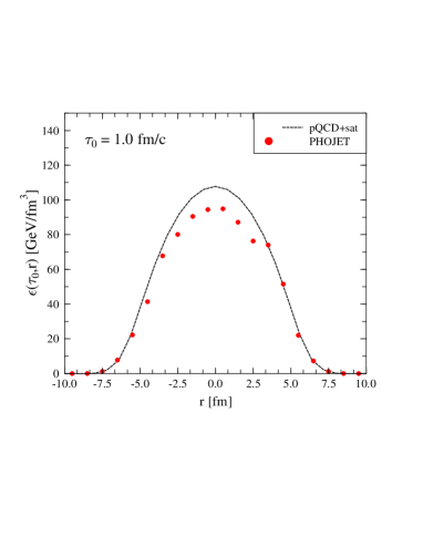
Figure 53: Transverse dependence of the energy density $\epsilon(\tau,r)$ at time $\tau=1.0$ fm/c from the pQCD+saturation model compared with results from the PHOJET calculation (circles) based on dual parton string model.

In the models based on initial state saturation, production is related to the number of participants which for central, zero-impact-parameter collisions is proportional to $T_{A}(r)$. Details in implementing the production dynamics may modify the transverse dependence but we will take the binary collision density $[T_{A}(r)]^{2}$ and the participant density $T_{A}(r)$ to represent the range of variation in the shape of transverse distribution of initial energy density.

We next consider the choice of initial time $\tau_{0}$ for the hydrodynamic evolution. In models based on parton production, the formation time scale of primary partons is the inverse of the saturation momentum, $\tau_{0}\sim 1/{p_{\rm sat}}$. However, as was discussed earlier, the time needed for the system to thermalize, $\tau_{\rm th}$, can be longer than the production time of partons [169, 170, 171], especially if the primary production is followed by fragmentation. Usually it is argued to indicate that thermal and hydrodynamical description of expansion cannot be started earlier than at $\tau_{\rm th}$. On the other hand, collisions drive the system towards equilibrium and they cannot be ignored since they contribute both to the buildup of collective motion and the emission of photons and lepton pairs even before full thermalization has been achieved. Applying hydrodynamics with initial time $\tau_{0}\sim\tau_{\rm prod}<\tau_{\rm th}$ means assuming that it provides a reasonable approximation for treating the effects due to collisions which drive the matter to thermal equilibrium. Especially, the high transverse momentum photons might otherwise be underestimated since the collision energies of partons are largest at the earliest stage.

In the pQCD + saturation model the assumption of early thermalization can be supported with two arguments: First, for the kinetic pressure and energy density of massless particles the relation $p=\epsilon/3$ holds for any isotropic momentum distribution. Second, in the pQCD + saturation model the number density and the energy density of produced partons is approximately consistent with the thermalization assumption. This would indicate that the collision rate can be similar to that in thermal system with the same energy density.

In the pQCD minijet calculation the saturation momentum at $\sqrt{s}=5.5$ TeV is 2.03 GeV giving $\tau_{0}=0.1$ fm/c. This is the earliest initial time to be used in exploring the photon emission.

Results for the multiplicity are very similar from the minijet model and the Dpmjet calculations as implied by the similarity of initial conditions, Fig. 53. They both give values $dN_{\rm ch}/dy\sim 3000$ for the total multiplicity and agree within the uncertainties of the models, like the choice of the saturation scale in the minijet calculation or the possible entropy generation after the primary production.

In the numerical evaluation of classical field equations the saturation scale is a parameter and the multiplicity changes with different choices of the scale.

Calculations based on the initial state saturation formulated in terms of the initial gluon densities [165] predict the energy dependence of the multiplicity and once the normalization is fixed from the RHIC data, the prediction for the charged multiplicity is around $dN_{\rm ch}/dy\sim 2200$ at LHC. Even though the authors indicate that, at least at RHIC, the evolution in final state, other than fragmentation, is not important, we exploit their result by considering an initial distribution $\propto T_{A}(r)$ normalized to fit the predicted multiplicity from their model.

Results from classical effective field theory on lattice in the transverse plane can change, depending on the choice of the saturation scale, by a large factor (order of 2 at RHIC energy) [163] for the parton multiplicity. The larger multiplicities are comparable with those from the minijet calculation and the lower ones lead to a final state similar to the one from the saturation calculation in terms of initial gluon distribution of incoming nuclei [165]. To get an idea how much the multiplicity may affect the photon emission we scale the initial conditions also upwards to cover the interval $2000\ \raise 1.29167pt\hbox{$<$\kern-7.5pt\raise-4.73611pt\hbox{$\sim$}}~{}\ dN_{\rm ch}/dy\ \raise 1.29167pt\hbox{$<$\kern-7.5pt\raise-4.73611pt\hbox{$\sim$}}\ 4000$ or from $\sim 3000$ to $\sim 6000$ in the total multiplicity.

Even though the final state energy density at $\tau=1$ fm/c from the Dpmjet model is quite similar to other calculations as shown in Fig. 53, it is not clear that the photon emission should be the same. In the Dpmjet calculation also strings are present in the final state and the space-time evolution might be very different from that of parton gas, predicted from the other calculations. Neither is it clear how well the use of the photon emission rates based on pQCD calculation with parton degrees of freedom apply if strings play an important role among the degrees of freedom in the final state.

To summarize: The two most important parameters for the determination of the initial state, the multiplicity $dN_{\rm ch}/dy$ and the initial timescale $\tau_{0}$, have a considerable range of uncertainty. Also the maximum values of the temperature in the final state are affected by the transverse shape of initial distributions and since the photon emission has a very strong temperature dependence, these effects are seen in the calculated photon spectrum. To estimate the uncertainty in the calculation of thermal photon emission we explore the following values of the input parameters for the initial conditions:

• $2000\ \raise 1.29167pt\hbox{$<$\kern-7.5pt\raise-4.73611pt\hbox{$\sim$}}\ dN_{\rm ch}/dy\ \raise 1.29167pt\hbox{$<$\kern-7.5pt\raise-4.73611pt\hbox{$\sim$}}\ 4000$,

• $0.1{\rm fm/c}\leq\tau_{0}\leq 1.0\ {\rm fm/c}$ and

• $\epsilon(\tau_{0},r)\propto[T_{A}(r)]^{\kappa}$ for $\kappa=1$ and 2.

6.6.3 Initial conditions and the evolution of fugacities

Gluon dominance in the initial production will lead to small (anti)quark fugacities. This turns out to have an important effect on the emission rates. At fixed temperature the decrease of fugacities leads to smaller densities which decreases the emission rate. However, at fixed energy density the decrease of fugacities increases the temperature which in turn increases the emission rate. Thus the effects from the lack of chemical equilibrium are complicated and the question if the emission rate increases or decreases can only be answered with a detailed calculation [176]. This means that we have to determine not only the initial values and the evolution of the temperature $T$ but also of the fugacities $\lambda_{g}$, and $\lambda_{q}$.

We determine the initial values of fugacities in the transverse plane at the initial time $\tau_{0}$ from the information on jet cross sections $\sigma_{g}$ and $\sigma_{q}\approx\sigma_{\bar{q}}$ and the cross section for transverse energy production, $\sigma\langle E_{{}_{T}}\rangle$. In doing so we also have to impose limits for the values of fugacities to assure thermodynamic consistency.

In Sec. 6.6.2 we constructed the initial energy density from $\sigma\langle E_{{}_{T}}\rangle$, Eq. (51). We can define the number densities of gluons and (anti)quarks, $n_{g}$ and $n_{q}$ respectively, in the same way by using $\sigma_{g}$ and $\sigma_{q}$ instead of $\sigma\langle E_{{}_{T}}\rangle$. If the temperature is known, the fugacities can be determined from the relation between the equilibrium thermal density $\hat{n}_{i}(T)$ and the real density $n_{i}$:

$$n_{i}=\lambda_{i}\hat{n}_{i}(T),\ i=g,q\,.$$ (52)

The equilibrium density $\hat{n}_{i}(T)$ is given as $\hat{n}_{i}=b_{i}T^{3}$ with $b_{g}=16\zeta(3)/\pi^{2},\ \zeta(3)=1.20206$ for gluons and $b_{q}=b_{\bar{q}}=9N_{f}\zeta(3)/2\pi^{2}$ for (anti)quarks. In fact, to determine the fugacities and the temperature the equations both for the number densities and the energy density, Eq. (47) must be solved simultaneously. An extra complication arises from the fugacity dependence of the bag constant $B$.

We will not go to all the details of solving the equations for the temperature and the fugacities here; it obviously can be done. However we must discuss the range of values for fugacities for which a consistent equation of state can be constructed. In Sec. 6.6.1 we stated a lower limit for the fugacities to ensure that the hadron gas will be the stable low temperature phase. It turns out that if we solve the fugacities and the temperature from the initial conditions using Eqs. (52) and (47) we will obtain, at the edges of the transverse nuclear overlap, fugacities which violate this condition. Also, in the central region of the transverse plane, gluon fugacities with values $\lambda_{g}>1$ are obtained. If the fugacity is written in terms of chemical potential, values exceeding one will lead to a singular unphysical phase space distribution function. To avoid this, we limit the gluon fugacity to be $\lambda_{g}\leq 1$. If solving the Eqs. (52) and (47) gives $\lambda_{g}>1$ we take $\lambda_{g}=1$ or equivalently $n_{g}=\hat{n}_{g}(T)$ and keep the quark fugacity unchanged. New temperature and number densities can then be recalculated using Eqs. (47) and (52). The lower limits at the edges of the nuclear overlap are imposed in the same way. It turns out that when these physically motivated limits are applied at the initial time, they are not violated by evolution of fugacities during the expansion on the parton matter.

Figure 54: Evolution of fugacities starting from the pQCD + saturation initial state. $\lambda_{g}(\tau,r)$ and $\lambda_{q}(\tau,r)$ are shown as function of time for $r=0$ and $r=6$ fm.

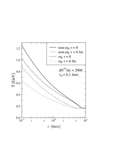
Figure 55: The evolution of temperature for the same situations as for the fugacities in Fig. 55.

The evolution of fugacities is determined by the rates of number changing reactions for gluons and quarks. There is a considerable uncertainty in the parton cross sections which are needed in the rate calculations. We follow the studies of Biró et al. [91] and Elliott and Rischke [92]) and include the processes $gg\to q\bar{q}$ and $gg\to ggg$ as well as their inverse reactions into the rate equations. The rate equations for the gluon and quark fugacities can be written as (see Eqs. (23) and (24) in Ref. [91])

$$\partial_{\mu}(\lambda_{i}\hat{n}_{i}(T)u^{\mu})=C_{i}(T,\lambda_{g},\lambda_{q})\,,\ \ i=g,q\,.$$ (53)

with the collision terms

$$C_{g} = \hat{n}_{g}R_{3}\lambda_{g}(1-\lambda_{g})-2\hat{n}_{g}R_{2}\lambda_{g}\left(1-\frac{\lambda_{q}\lambda_{\bar{q}}}{\lambda_{g}^{2}}\right)\,,$$ (54)

$$C_{q} = \hat{n}_{g}R_{2}\lambda_{g}\left(1-\frac{\lambda_{q}\lambda_{\bar{q}}}{\lambda_{g}^{2}}\right)\,,$$ (55)

where, even though we have taken $\lambda_{q}=\lambda_{\bar{q}}$, we have written the quark and antiquark fugacities explicitly to show the origin of different terms. For the rate parameters $R_{i}$ we use the results derived in [91]:

$$R_{2} \approx 0.24N_{f}\alpha_{s}^{2}\lambda_{g}T\ln(1.65/\alpha_{s}\lambda_{g})\,,$$ (56)

$$R_{3} = 1.2\alpha_{s}^{2}T(2\lambda_{g}-\lambda_{g}^{2})^{1/2}\,.$$ (57)

Equations (53-57) are solved numerically simultaneously with the hydrodynamic equations and the change in the EoS due to the change in fugacities is included in the calculation.

In the beginning of the expansion with large parton densities the evolution towards thermal equilibrium is fast but it slows down as the matter expands and rarefies. In Fig. 55 we show the time dependence of the fugacities in the parton matter at $r=0$ and $r=6$ fm starting from the pQCD + saturation initial state at $\tau_{0}=0.1$ fm/c. At $r=0$ gluon fugacity $\lambda_{g}=1$, but since the number of quarks and antiquarks is small, the rate for $gg\to q\bar{q}$ reduces the number of gluons faster than the the inverse reaction and reaction $gg\to ggg$ can balance it.

The evolution of fugacities affects also the evolution of the temperature. In Fig. 55 the temperature is shown as function of time for the same conditions as the fugacities in Fig. 55. To see the significance of the lack of chemical equilibrium, we show the evolution of the temperature for the same initial conditions also when full equilibrium is assumed. Initially the temperature is higher when the matter is out of chemical equilibrium. This happens because the effective number of degrees of freedom is $16\lambda{}_{g}+21N_{f}\lambda_{q}/2$ instead of $16+21N_{f}/2$ of the equilibrium case. As the number of effective degrees of freedom increases with time the temperature drops faster in non-equilibrium matter and approaches that in equilibrium matter. However, as will be seen below, from the point of view of photon emission, the higher initial temperature turns out to approximately compensate for the lower parton densities.

6.7 Hadron spectra from a hydrodynamical calculation

H.Niemi, P.V. Ruuskanen, S.S. Räsänen

The calculations of hadron and photon spectra proceed somewhat differently. Since the mean free paths of photons are larger than the size of the fireball, they are emitted throughout the expansion of matter from the whole thermal volume. Hadrons escape only from the surface of the fireball or after the density in the whole volume is so small that no further interactions take place. We first consider the hadrons and then the photons.

As the matter expands, distances between particles become large, collisions cease and momentum distributions freeze out. The condition for the freeze-out to happen is usually expressed locally in terms of the energy density or temperature reaching a given value. This determines a three-dimensional freeze-out surface $\sigma^{\mu}(x)$ in space–time. The prescription of Cooper and Frye [177] to convolute the flow and the thermal motion along the freeze-out surface

$$\pi{dN\over d^{3}{\bf p}/E} = {dN\over dydp_{{}_{T}}^{2}}=\pi\int_{\sigma}d\sigma_{\mu}(x)p^{\mu}f(x,p;T(x))$$ (59)

$$= {g\over 2\pi}\sum_{n=1}^{\infty}(\pm 1)^{n+1}\int_{\sigma}r\tau\big{[}-p_{{}_{T}}I_{1}(n\gamma_{r}v_{r}{p_{{}_{T}}\over T})K_{0}(n\gamma_{r}{m_{T}\over T})\,d\tau$$

$$+m_{T}I_{0}(n\gamma_{r}v_{r}{p_{{}_{T}}\over T})K_{1}(n\gamma_{r}{m_{T}\over T})\,dr\big{]}\,,$$

is used to calculate first the spectra of all hadrons and hadron resonances. The second expression above is valid for cylindrically symmetric, boost invariant flow with $v_{r}$ the radial flow velocity, $\gamma_{r}=1/\sqrt{1-v_{r}^{2}}$, and $K_{0}$ and $I_{0}$ Bessel functions. We then follow the chains of all possible two and three body decays and collect the spectra of final stable hadrons. The stable hadrons can be interpreted as the absolutely stable hadrons or also those with weak decays or both weak and electromagnetic decays. The treatment of hadrons with weak decays can be important, e.g. in the case of $\Lambda$’s, depending if the measurement can separate the feed-down from heavy hyperons or not. Electromagnetic decays, as a source of photons, are of special interest but we display later also the spectrum of $\pi^{0}$’s before their decay.

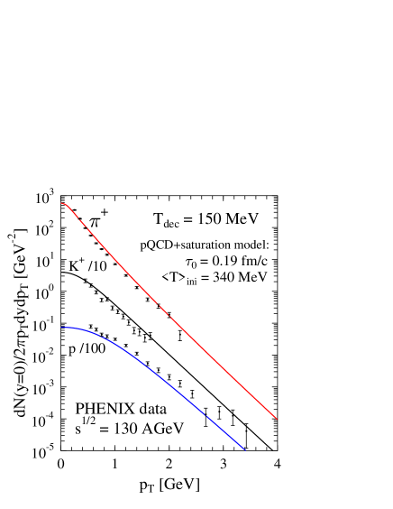
Figure 56: Transverse momentum spectra of positive pions, kaons and protons measured by PHENIX Collaboration at $\sqrt{s}=130$ GeV shown with results from a hydrodynamical calculation with initial conditions from the pQCD + saturation model.

Since the transverse momentum distribution of the decay photons depends strongly on the transverse spectra of hadrons, we show in Fig. 56 the measured spectra of positive pions, kaons and protons at RHIC [178] with results from a hydrodynamical calculation using the initial conditions from the pQCD + saturation model [145]. The results describe the data quite well at small momenta, but it is clear that a hydrodynamic calculation cannot describe the hadron spectra at transverse momenta larger than $\sim 4-5$ GeV. The fraction of hadrons with $p_{{}_{T}}\raise 1.29167pt\hbox{$>$\kern-7.5pt\raise-4.73611pt\hbox{$\sim$}}5$ GeV from all hadrons is small and in thermal models the dominant fraction of low transverse momentum hadrons is assumed to come from the thermalized matter with collective motion. From this point of view the calculation of decay photons using the hadron spectra from a hydrodynamical calculation gives a reasonable estimate in the range of low momenta, say up to $p_{{}_{T}}\sim 3-4$ GeV.

Similarly, the spectra of hadrons from the thermal fireball at LHC energy can be calculated for any given choice of initial conditions. As an example of hadron spectra at LHC we show here the spectra of positive pions and kaons and protons in Fig. 57 obtained with initial conditions from the pQCD + saturation model [179] which, as already pointed out above, reproduce well the data at RHIC. To show the uncertainty in the shape due to the decoupling procedure, results with decoupling temperatures ${T_{\rm dec}}=120$ and 150 MeV are displayed. All spectra become flatter at later decoupling and the role of the flow is seen from the change getting larger with increasing mass. We will show later how this uncertainty is transferred to the spectrum of photons from hadron decays.

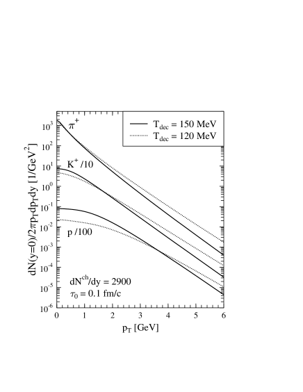
Figure 57: Transverse momentum spectra of positive pions, kaons and protons calculated at $\sqrt{s}=5.5$ TeV from the pQCD + saturation initial conditions [179]. The two sets of curves correspond to two different choices of decoupling temperature, ${T_{\rm dec}}=120$ and 150 MeV.

Note that even though the range of parametrization of initial conditions have been motivated by different model calculations it does not mean that such spectra are predictions by the authors of these models in some of which hydrodynamic expansion may not be needed at all. When using a thermal model for describing the hadron spectra and the electromagnetic emission we have used these calculations to argue what could be the reasonable range of input parameters and we always make the assumption that there is a hydrodynamical expansion stage between the primary production and the formation of final hadrons. As reviewed in Sec. 6.5.2, e.g. in [165] no thermal stage is assumed to occur.

6.8 Spectra of thermal photons

H. Niemi, P.V. Ruuskanen, S.S. Räsänen, D.K. Srivastava

The photon spectra are obtained by integrating the emission rate over the whole space–time volume of the fireball. We use the emission rates which are discussed in detail in Secs. 6.2 for the equilibrium QGP, in Sec. 6.3 for the QGP in kinetic equilibrium but out-of-chemical equilibrium and in 6.4 for the hadron resonance gas.

The local emission rate is a function of the local temperature and the energy of the photon in the rest system of the matter, $dN(\omega^{*},T)/d^{4}x$. In the case of flowing matter this is the co-moving frame of the fluid element. If $p^{\mu}=(E,\tenimbf p)$ is the four–momentum of the photon in the fixed frame where the photon is observed and $u^{\mu}$ the four–velocity of the emitting fluid element in that frame, the energy of the photon in the co-moving frame is $\omega^{*}=p\!\cdot\!u=p_{\mu}u^{\mu}$. Since $d^{3}{\tenimbf p}/E$ is Lorentz invariant, we obtain

$$E\frac{dN_{\gamma}}{d^{3}{\tenimbf p}}=\int d^{4}x\frac{dN(\omega^{*},T)}{d^{4}x\ {d^{3}{\tenimbf p}/E}}\,.$$ (60)

At the transition temperature $T_{c}$ the matter may enter into a mixed phase which is characterized by the volume fractions of each phase. In the mixed phase the emission rate is taken to be the sum of rates in QGP and hadron gas at $T=T_{c}$, weighted with the volume fraction of the phase.

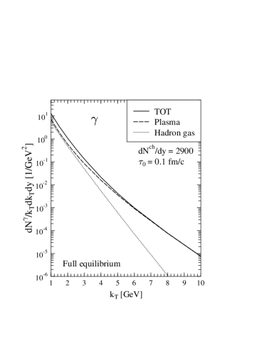
Figure 58: Our baseline spectrum of thermal photons: full equilibrium with EoS A, $dN_{\rm ch}/dy=2900$ and $\tau_{0}=0.1$ fm/c. Contributions from plasma and hadron gas are shown separately.

We next consider the photon spectra which are obtained when $u^{\mu}(r,\tau)$ and $T(r,\tau)$ are calculated using different initial conditions and equations of state. We start with the spectrum, shown in Fig. 58, from the minijet calculation with the pQCD + saturation model, used as a baseline and plotted in most of the figures to facilitate the comparison of different results. In this baseline case we assume full equilibrium in the plasma phase, both kinetic and chemical, the charged multiplicity is $dN_{~{}\rm ch}/dy=2900$ and we have taken $\tau_{0}=1/{p_{\rm sat}}\approx 0.1$ fm/c. A similar calculation at RHIC energy, $\sqrt{s}=$ 200 GeV has been presented in Ref. [180].

The large-$p_{{}_{T}}$ region of the spectrum is completely dominated by the emission from plasma during a short period at earliest times. The transverse flow plays no role at that time and the slope is determined by temperatures close to the maximum temperature. With these initial conditions plasma gives the main contribution also at smaller values of transverse momentum. Photons from the hadron gas phase have a much steeper slope than those from QGP. This slope is not given by the temperature of the hadron phase alone but by the combination of temperature and the flow. Actually the situation is quite similar with that of the hadron spectra. This is shown by the fact that the slope of the (almost massless) pions in Fig. 57 is very close to that of photons from hadron phase in Fig. 58.

Figure 59: Thermal photon spectra in Pb+Pb collisions at LHC energy for different charged hadron multiplicity assuming full thermal equilibrium throughout the expansion.

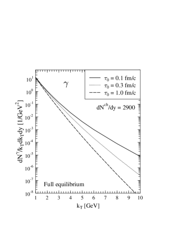
Figure 60: As in Fig. 60 but as a function of initial time $\tau_{0}$ for fixed charged multiplicity $dN_{\rm ch}/dy=2900$.

In Fig. 60 spectra of thermal photons are shown for charged multiplicities $dN_{~{}\rm ch}/dy=1900,\ 2900$ and 3800. To see the effect from the change of the multiplicity alone, same value $\tau_{~{}0}=0.1$ fm/c for the initial time has been used in each case. As will be seen later, the transverse momentum window of interest for observing thermal photons may extend from $p_{{}_{T}}\sim$ 2 GeV up to $p_{{}_{T}}\sim 10$ GeV in the favourable case. A change in charged particle multiplicity from 1900 to 3800 increases the photon rate by more than a factor of five at the lower end and almost a factor of 10 at the upper end of the interval. Since the dependence of decay photons is close to linear in hadron multiplicity, a strong dependence on the multiplicity in the relative strength of thermal photons to those from hadronic sources can be expected.

A large uncertainty in the photon emission comes from the uncertainty on the production and thermalization times of the initial partons. In all production calculations based on QCD the initial state is dominated by gluons due to the SU(3) properties of the couplings among gluons and (anti)quarks. Thus the system is far from chemical equilibrium after the production stage. It may also be far from kinetic equilibrium and there are arguments that equilibrium is reached only on a timescale of 2…3 fm/c [169, 170, 171]. We will consider the chemical equilibration separately below. Here we just consider the effect of the initial time $\tau_{~{}0}$ in the hydrodynamical calculation.

We already argued in favour of a shorter timescale for the initial time of hydrodynamic expansion, $\tau_{0}$, than obtained from the thermalization arguments. In a parton-based approach the production timescale is provided by the momentum scale at which the production is expected to saturate, $\tau_{\rm prod}\sim 1/{p_{\rm sat}}$. The momentum distribution will not be thermal initially but the partons can scatter from the time $\tau_{\rm prod}$ on and some of these interactions produce photons. A kinetic calculation of photon emission starting from different initial distributions would be better justified but we would like to argue that by taking $\tau_{0}=\tau_{\rm prod}$ we effectively simulate the photon emission also from those interactions which bring the matter towards kinetic equilibrium. In Fig. 60 we show the variation when the initial time is changed. It is seen to be very strong at large $p_{{}_{T}}$ as is expected since the magnitude of local relative momenta or, in the thermodynamic language, the temperature decreases rapidly due to the longitudinal expansion.

When we compare these spectra with photons from other sources, we will see that the observation of thermal photons, or more generally photons from secondary collisions among initially produced partons, is possible only if the produced partons can begin to scatter at early times immediately after production when they still have large relative momenta.

Figure 61: Photon spectra when the shape of initial condition is is taken to be $[T_{A}(r)]^{\alpha}$ with $\alpha=1$ or 2. $dN_{\rm ch}/dy\simeq 2900$ and $\tau_{0}=0.1$ fm/c in both cases.

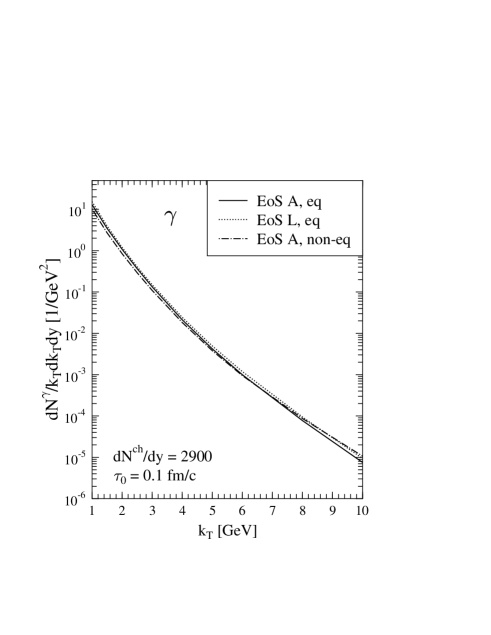
Figure 62: Our baseline result (solid line) is shown with the the photon spectrum for an out of chemical equilibrium calculation (dashed-dotted line) and for a calculation using the lattice EoS (dotted line). In all cases $dN_{\rm ch}/dy\simeq 2900$ and $\tau_{0}=0.1$ fm/c.

In calculating the spectra in Figs. 60 and 60 we have assumed that the radial dependence of initial distributions is proportional to $[T_{A}(r)]^{\alpha},\ \alpha=2$. Fig. 62 shows the difference between the cases $\alpha=$ 1 and 2. With $\alpha=2$ the distribution is steeper and more peaked in the center than in the case $\alpha=1$. Consequently, for fixed multiplicity the maximum temperature is higher in the former case and the strong temperature dependence of emission rate leads to stronger overall emission and more shallow dependence on $p_{{}_{T}}$ of the spectrum.

We next discuss how the deviation from chemical equilibrium affects the photon emission. The initial values and the evolution of fugacities are determined as described in Sec. 6.6.3. When the values of fugacities are less than one, $\lambda_{i}<1$, the numbers of degrees of freedom are effectively less than in plasma in full equilibrium. Comparing with the equilibrium case at a given energy density, parton densities are smaller but temperatures higher. For the photon emission spectrum, it turns out that the increase in temperature approximately compensates the decrease of parton densities, over the $p_{{}_{T}}$ range considered.

In Fig. 62 we compare our baseline case in full equilibrium with the non-equilibrium case specified in Sec. 6.6.3. In both cases the charged particle multiplicity is 2900 and the initial time $\tau_{~{}0}=0.1$ fm/c. The spectra approximately coincide, the off equilibrium case giving slightly smaller results at small $p_{{}_{T}}$ and about 20% higher at $p_{{}_{T}}\raise 1.29167pt\hbox{$>$\kern-7.5pt\raise-4.73611pt\hbox{$\sim$}}10$ GeV.

We also show in Fig. 62 the result of a calculation using an equation of state with the high temperature phase fitted to the lattice data. The calculation starts from the same initial conditions as in the baseline case. As is seen in Fig. 52, the lattice parametrization corresponds to higher temperature at given energy density than our EoS A. In the photon spectrum this shows up as a slight increase in the photon emission. There are indications that if lattice results are interpreted in terms of quasiparticle excitations, the quasiparticle masses do not exactly correspond to the thermal masses of partons. The photon emission is calculated with the standard perturbative rates but it might be more consistent to replace the thermal masses in the rates with the (temperature dependent) quasiparticle masses obtained from the lattice information.

Recently an interesting new photon source was proposed [181]. It is an outcome of the interactions of energetic jets with the thermalized plasma. The idea is similar to that in jet quenching: the bulk of the plasma comes from partons close to the saturation momentum but the high energy partons do not thermalize. They will traverse the matter interacting with its quanta. In some of these interactions photons will be emitted and if the properties of matter and the cross section for photon production are known, the emission rate can be calculated.

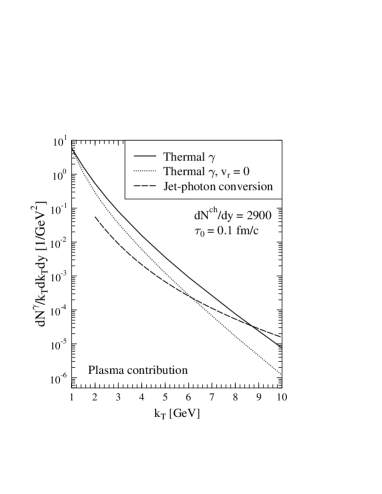
Figure 63: Photons from jets interacting with plasma. Thermal photons dominate at small $p_{{}_{T}}$ but have a steeper slope than those from jets. Since the jet + plasma calculation is performed with $v_{r}=0$, we show also the thermal spectrum in that case.

In Fig. 63 the spectrum of photons emitted from jets traversing the plasma is compared with our baseline thermal spectrum. The calculations of jets interacting with plasma has been performed in the case of no transverse expansion and this complicates the comparison with the results from thermal emission. In any case, the emission from jet + plasma interactions is related to the existence of plasma; it is not a competing signal with thermal emission but they add together, enhancing the possibility to observe a photon excess due to the formation of plasma.

6.9 Comparing thermal and decay photons in a hydrodynamical model

H. Niemi, P.V. Ruuskanen, S.S. Räsänen

Hadron decays, in particular those of $\pi^{0}$’s, form the most copious source of photons. In this section we show the photon spectra from the hadron decays when the hadron spectra are obtained from the hydrodynamical calculation and compare them with the spectra of thermal photons. The decay photons from all hadrons in the EoS are included. In a hydrodynamical model the thermalized part of produced matter is assumed to dominate the multiplicity and the transverse momentum distributions up to few GeV. A hard parton, say $p_{{}_{T}}\raise 1.29167pt\hbox{$>$\kern-7.5pt\raise-4.73611pt\hbox{$\sim$}}10$ GeV will not thermalize but in traversing the thermal part of matter it may loose energy before fragmenting into the jet of final hadrons. The loss of energy of these hard partons leads to a shift to smaller transverse momenta of the large-$p_{{}_{T}}$ hadrons. The jets still dominate at large transverse momentum part of the hadron spectra. In this picture decay photons with $p_{{}_{T}}\raise 1.29167pt\hbox{$<$\kern-7.5pt\raise-4.73611pt\hbox{$\sim$}}2-4$ GeV come from the hydrodynamic part of the hadron spectra and the large-$p_{{}_{T}}$ photons from hadrons produced in jets. There is no obvious way to join the two regions smoothly since there is no well-defined way to cut off the jet calculation at low transverse momenta.

Figure 64: Spectra of (i) $\pi^{0}$’s (dashed), (ii) decay photons from these $\pi^{0}$’s (dotted) and (iii) thermal photons (solid line: full equilibrium; dash-dotted line: off chemical equilibrium) from a hydrodynamical calculation with initial conditions from a minijet calculation at $\sqrt{s}=200$ GeV. Also the $\pi^{0}$ spectrum, measured by the PHENIX collaboration is shown.

Figure 65: As in Fig. 65 but at $\sqrt{s}=5.5$ TeV. The bands for $\pi^{0}$’s and decay photons are shown for ${T_{\rm dec}}=120$ (upper) and 150 (lower) MeV. The predictions for thermal photons with full chemical equilibrium and off chemical equilibrium cannot be distinguished and are shown by the solid line.

We would like to remind that in the hydrodynamical model thermal photons are emitted throughout the expansion of the produced fireball whereas the final hadrons emerge only from rarefied low-temperature matter on the decoupling hyper surface. Consequently the large transverse momentum photons and hadrons come from different regions of the fireball: high-$p_{{}_{T}}$ photons are emitted at the earliest times from the initial quark-gluon matter at highest temperature reached in the interior of the fireball. On the other hand, the strong flow develops at the surface of expanding matter and the large-$p_{{}_{T}}$ hadrons originate from the fastest matter at the edge of the fireball. Expressed differently, the slope of the tail of thermal photon spectrum is determined by the highest values of the initial temperature in the interior of the matter but those of hadron spectra by the fastest flow on the surface of the matter.

We show the calculation from the minijet initial conditions only. The initial time is $\tau_{~{}0}=1/p_{\rm sat}$, equal to $0.1$ fm/c at the LHC energy, $\sqrt{s}=5.5$ TeV, and $0.18$ fm/c at the RHIC energy, $\sqrt{s}=200$ GeV. As is seen from Fig. 65, the magnitude of the calculated $\pi^{0}$ spectrum agrees with that of the measured one for $p_{{}_{T}}\raise 1.29167pt\hbox{$<$\kern-7.5pt\raise-4.73611pt\hbox{$\sim$}}3$ GeV. Above this region the shallow tail of $\pi^{0}$’s comes from the jet fragmentation. The spectra of decay and thermal photons cross at $p_{{}_{T}}\simeq~{}4.5$ GeV at RHIC.

Results at the LHC energy are shown in Fig. 65. The spectra of $\pi^{0}$’s and the decay photons are shown for two decoupling temperatures. The lower decoupling temperature, ${T_{\rm dec}}=120$ MeV gives the upper boundaries and the higher ${T_{\rm dec}}=150$ MeV the lower ones. The solid line shows the thermal photon spectrum for both the full chemical equilibrium and the off equilibrium cases: they cannot be distinguished. This curve is, of course, not the lower limit for the thermal photon emission. For example, as is seen from Figs. 60 and 60, thermal production depends very strongly on the assumptions made of the initial conditions. In the case of Fig. 65 the thermal and decay photons cross at $\sim 5$ GeV and for $p_{{}_{T}}\raise 1.29167pt\hbox{$<$\kern-7.5pt\raise-4.73611pt\hbox{$\sim$}}~{}2$ GeV the amount of decay photons is more than 10 times the number of thermal photons. Depending on the amount of $\pi^{0}$’s from jet fragmentation a window with thermal photons of the order of 10 % of the background could exist in the region of $p_{{}_{T}}$ above 2-3 GeV. All sources of photons, thermal, prompt pQCD from primary interactions between incoming partons, and decays of both the thermal and jet hadrons, are compared in the next section.

6.10 Thermal small mass lepton pairs

P. Aurenche, F. Gelis, H. Niemi, P.V. Ruuskanen and S.S. Räsänen

Like real photons, also virtual photons, decaying to lepton pairs, can be emitted during the thermal stage of collisions. As mentioned in sec. 6.2.2 the dynamics of production of a small mass pair at large momentum is similar to that of a real photon and experimentally this channel provides a complementary signature to real photon production.

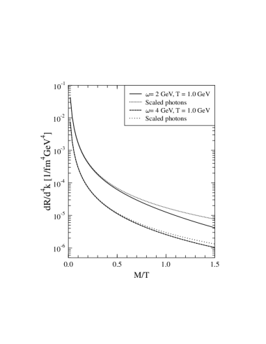
Figure 66: Emission rates for lepton pairs as function of $M/T$ are compared with the photon emission rate scaled with $\alpha/3\pi M^{2}$ (dotted lines) for $E=\omega=2.0$ (solid line) and 4.0 GeV (dashed line).

From Eq. (18) and Eq. (24) one can derive the approximate scaling relation which should hold true when the virtual photon mass becomes small compared to all other scales in the problem:

$${{dN_{{}_{l^{+}l^{-}}}}\over{dtd^{3}{\tenimbf x}\ dM^{2}d^{3}{\tenimbf p}}} = {{dN_{{}_{l^{+}l^{-}}}}\over{dtd^{3}{\tenimbf x}\ 2EdEd^{3}{\tenimbf p}}}$$ (61)

$$\simeq {\alpha\over\pi M^{2}}\;{{dN_{{}_{\gamma}}}\over{dtd^{3}{\tenimbf x}\ d^{3}{\tenimbf p}}}$$ (62)

where $P=(E,{\tenimbf p})$ and $P^{2}=M^{2}$ for the lepton pair.

In Fig. 66 the dilepton rate for $E=2$ and 4 GeV at $T=0.5$ GeV is shown as a function of $M/T$ and compared to the scaled photon rate at the same energies $E$. It is seen that for the pair mass up to 0.5 GeV/c² the scaling works very well. The scaling holds true also for the emission from the plasma integrated over its whole expansion time in the nucleus-nucleus collision. This is shown in Fig. 68 for the transverse distribution at different values of the pair mass. Even for $M=0.5$ GeV/c² the scaling works well except for the small-$p_{{}_{T}}$ region where the ratio $M/E$ becomes large and, as expected, the scaling formula overestimates the rate.

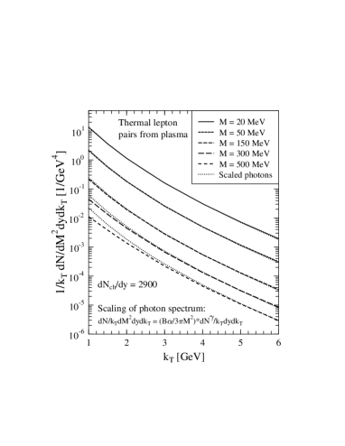
Figure 67: Transverse spectra for thermally emitted pairs from the plasma phase in a Pb+Pb collision at LHC for charged multiplicity $dN_{\rm ch}/dy=2900$. Photon spectrum from the same hydrodynamical calculation with emission rate scaled according to Eq. 62.

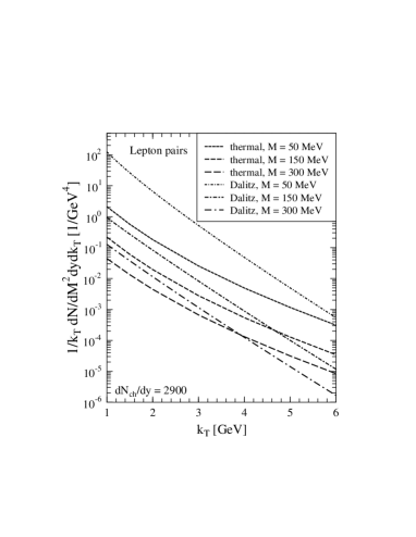
Figure 68: Dalitz pairs from $\eta$ and $\pi^{0}$ compared with thermal pairs in a Pb+Pb collision at LHC with $dN_{\rm ch}/dy=2900$. The spectra of $\eta$’s and $\pi^{0}$’s are obtained from the same hydrodynamical calculation as the thermally emitted pairs.

For small-mass pairs between 0.2 and 0.4 GeV/c² the dominant background comes from the Dalitz decays of $\eta$’s. For $M\sim 0.4-0.5$ GeV/c² pairs from $\eta^{\prime}\to ee\gamma$, $\omega\to ee\pi^{0}$ and direct vector meson decays become comparable and for larger masses (up to 1 GeV/c²) dominant. To get an idea of the relative size of the thermal and background contributions we calculate the Dalitz pairs using for $\pi^{0}$’s and $\eta$’s the spectra obtained from the hydrodynamic calculation. For the Dalitz decay distribution we use [182, 183] the form

$$\frac{d\Gamma^{a}}{dM}=\frac{4\alpha}{3\pi}\frac{\Gamma(a\to\gamma\gamma)}{M}\left(1-\frac{M^{2}}{m_{a}^{2}}\right)^{2}\left(1+\frac{2m_{e}^{2}}{M^{2}}\right)\left(1-\frac{4m_{e}^{2}}{M^{2}}\right)^{1/2}$$ (63)

which, when integrated over the pair mass, reproduces well the measured branching ratios [184].

In Fig. 68 thermally emitted lepton pairs are compared with Dalitz pairs for three different mass values. At the smallest mass value, $M=50$ MeV/c², the Dalitz pairs are dominated by those from $\pi^{0}$ decays and they are well above the thermal rate. The situation with the relative size of thermal and decay contributions is qualitatively the same as in the case of real photons, see Fig. 65. For the mass values above the $\pi^{0}$ mass it becomes more favourable. Even at small transverse momentum, the ratio of Dalitz to thermal pairs is at most 5 and the contributions cross at $p_{{}_{T}}\sim 4-5$ GeV/c.

It should be noticed that the discussion here concerns the correlated pairs only. Since the multiplicity of neutral pions is expected to be more than 1000, the number of Dalitz pairs from $\pi^{0}$ decays with the 0.012 branching ratio will be $\sim 15$ per unit rapidity. In the experiment it is not possible to identify unambiguously if both particles of an observed $e^{+}e^{-}$ pair came from the same decay or from a single thermal emission (correlated pair), or if they came from a different interaction, either decay or thermal, and would constitute an uncorrelated pair. The number of observed uncorrelated pairs goes like $\sim N_{\rm pair}(N_{\rm pair}-1)$ and therefore should rapidly decrease with $p_{{}_{T}}$. An estimate of the uncorrelated background was already discussed in sec. 5.6 in the context of the Dpmjet model. In principle, the subtraction of the uncorrelated pairs can be done on statistical basis (using like-sign pairs) but the available overall intensities may limit the accuracy and consequently the minimum signal-to-background ratio for resolving the signal. Since the decays from the same hadrons produce the background both for photons and small-mass lepton pairs, the simultaneous measurement of photons and leptons, or any independent measurement on $\pi^{0}$ and $\eta$ spectra, can be used to improve the background subtraction.

7 COMPARING $\pi^{0}$’s AND PHOTONS FROM DIFFERENT SOURCES

P. Aurenche, H. Delagrange and P.V. Ruuskanen

In this Chapter we present a compilation of the results of Chapters 5 and 6 and we compare the strength of different sources of $\pi^{~{}0}$’s and photons. For the reader’s convenience, we briefly summarize the features of each of the three models we have considered:
– Dpmjet which is able to deal with the whole $p_{{}_{T}}$ spectrum, down to $p_{{}_{T}}=0$, as it contains both soft physics (string formation) and pQCD physics in the LO approximation. In A+A collisions a high density of soft strings is produced and final state interactions are taken into account by fusion and percolation of strings. The parameter determining this feature has been fitted to RHIC data. No reference to final state energy loss is needed in this approach;
– Standard NLO QCD calculations which are valid at “high” $p_{{}_{T}}$ only, where “high” is arbitrarily chosen to be $p_{{}_{T}}>3$ GeV/c: this rather low value for LHC is justified by the fact that DGLAP physics seems to hold true down to low $x$ values, and more practically, because down to 3 GeV/c Dpmjet and NLO predictions are still in good agreement. The NLO predictions describe the “primary” collisions modified, in the case of A+A scattering, by shadowing and energy loss;
– Hydrodynamic evolution of the quark-gluon plasma and hot hadronic matter during which hadrons and photons are produced essentially at low transverse momentum. This is refered to as “secondary” particle production.

We naively expect to obtain a full description of a nucleus-nucleus collision by adding the NLO contribution to the QGP and hot hadronic matter contributions which describe secondary interactions. We therefore have at our disposal two alternative models: Dpmjet and “NLO QCD + Hydro” (the “standard approach”) to make predictions which we are now going to discuss.

Since the photons from the decays of hadrons, in particular from $\pi^{~{}0}$’s, form a background which is larger than the total emission from all other photon sources we begin by comparing the spectra of $\pi^{~{}0}$’s calculated assuming different production mechanisms. In the second part of the Chapter we present the compilation and comparison of photon spectra from different sources and discuss the implications on the possibility to observe different dynamical features, such as the production mechanism and the equilibration, which are believed to be important in the formation and evolution of matter in lead–lead collisions at LHC. A third part briefly deals with lepton pair production.

7.1 Features of neutral pion spectra

Hadrons at large transverse momenta originate from hard collisions of incoming energetic partons followed by the formation of hadron jets through the fragmentation of scattered partons. In proton-proton collisions this is firmly established and it should also take place in nucleus-nucleus collisions. However, as discussed in Chapter 5, nuclear effects like shadowing, energy loss in traversing the system of other produced quanta and possible collective effects are expected to be important and to modify the spectra from those in hadron-hadron collisions. Most extreme of these modifications would be the thermalization of all produced quanta. However, this is unlikely on theoretical grounds from estimates of energy loss and the experimental results at RHIC [2, 3, 6] clearly show the persistence of the high transverse momentum tails in hadron spectra. These measurements also show a clear change in the shape of spectra indicating the energy loss of jet-generating partons in the final state.

On the other hand the very fact of energy loss of high energy partons in the final state points to the equilibration of lower energy partons. An interesting question is the characterization of the energy region where the transition from partons able to traverse the whole final state to those stopping and participating to the collective behaviour of the rest of produced matter takes place. It should be remembered that the high energy partons, say $p_{{}_{T}}\raise 1.29167pt\hbox{$>$\kern-7.5pt\raise-4.73611pt\hbox{$\sim$}}10$ GeV/c, leading to the jet formation, carry only a small fraction of the energy of all final state particles. This facilitates the hydrodynamic modelling since it should be a good approximation to assume that all the energy is equilibrated.

In the following we summarize the results of the previous chapters by showing those from each calculation which are estimated as the most likely. The results for $\pi^{0}$ production at RHIC are shown in Fig. 69. This figure is the same as Fig. 32 to which we have added the $p_{{}_{T}}$ spectrum originating from thermal production. At around $p_{{}_{T}}=3$ GeV/c the rapidly falling thermal spectrum crosses the NLO QCD one which is somewhat below the experimental points. The thermal spectrum agrees with the data at $p_{{}_{T}}<3$ GeV/c while the NLO QCD predictions agree with the data above $p_{{}_{T}}\sim 4$ GeV/c where thermal production becomes irrelevant. It thus appears that the “NLO QCD + Hydro” picture gives a very reasonable agreement with data at 200 GeV/c as does Dpmjet. These two models are therefore good starting points for extrapolation to LHC energies.

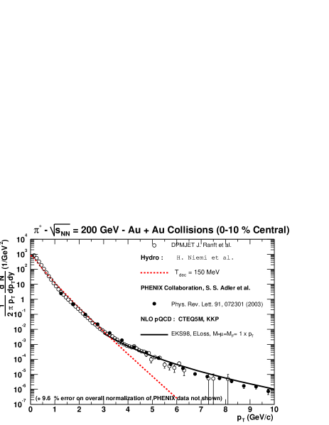
Figure 69: Spectra of $\pi^{0}$’s in Au+Au collisions at $\sqrt{s}=200$ GeV shown for the following calculations: (i) pQCD jet production and fragmentation (solid line), (ii) Dpmjet model (open circles), and (iii) pQCD+saturation for production followed by hydrodynamics with decoupling at $T_{\rm dec}=150$ (dashed line).

In Fig. 70 we show the results at $\sqrt{s}=5.5$ TeV. We display: the Dpmjet model $\pi^{0}$ predictions (open circles), the spectra from the NLO perturbative QCD calculation (solid line) and from the hydrodynamical calculation with full thermalization (freeze-out at $T_{\rm~{}dec}=120$ MeV, dotted line and 150 MeV, dashed line). The basic input parameters for pQCD calculation (including shadowing and energy loss) are summarized in the figure (see Chapter 5 for more details and in particular Fig. 33). The effect of the choice of renormalization and factorization scales is shown as a shaded band.

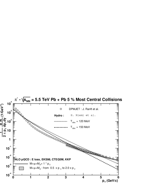
Figure 70: Spectra of $\pi^{0}$’s in Pb+Pb collisions at $\sqrt{s}=5.5$ TeV. The following calculations are shown: (i) pQCD jet production and fragmentation (solid line with the grey band), (ii) Dpmjet model (open circles), and (iii) pQCD+saturation for production followed by hydrodynamics with decoupling at $T_{\rm dec}=120$ (dotted line) and 150 MeV (dashed line).

The results from hydrodynamics dominate the spectrum at low $p_{{}_{T}}$ possibly up to intermediate momenta 4 …5 GeV/c where they cross below the NLO QCD predictions. So the transverse momentum regions where pQCD calculations or the hydrodynamic description apply are complementary. The full prediction in the “NLO QCD + Hydro” is the sum of the two curves but unfortunately, there is no clear way to join the two smoothly. It seems that the difference in slopes is so large that the region of crossing is quite stable against the uncertainties in the calculations. At large transverse momenta the Dpmjet results agree quite well with the pQCD calculation up to the highest values where the models have been compared, as can be seen in Fig. 33: this agreement occurs despite the fact that the two models have very different mechanisms to describe the interaction of jets with hot matter.

One can note the rather different shape of the $p_{{}_{T}}$ distributions, in the range 0 to 5 Gev/c, between the two approaches. Interestingly, the Dpmjet results show an even stronger change of slope than that from the high–$p_{{}_{T}}$ pQCD region and the low–$p_{{}_{T}}$ hydrodynamic region. The change also occurs at lower momenta, around 1…2 GeV/c, and the small-$p_{{}_{T}}$ part is much steeper than that obtained from the hydrodynamic calculation. If the final multiplicity (the total particle multiplicity from the hydrodynamic calculation $\sim 4500$) is as high as or close to what follows from the pQCD + saturation model initial conditions, it seems difficult to obtain such a steep slope from a hydrodynamical calculation. The reason for this is that it takes a long time to dilute the dense initial energy of a high-multiplicity collision; a strong transverse collective flow has time to build up and boost the particles to high transverse momenta even in case of relatively low thermal momenta at freeze-out. These differences show that the shape of the transverse momentum spectra of hadrons, even at relatively low transverse momenta, contains important information on the dynamics in the nucleus–nucleus collision. These differences in shape are much more marked at LHC than at RHIC.

7.2 Comparing photon spectra from main sources

Photon spectra from different sources are shown in Figs. 71 and 72 for RHIC and LHC, respectively. The figures are more complicated than in the case of pions since photons can be produced either directly or through the decay of hadrons.

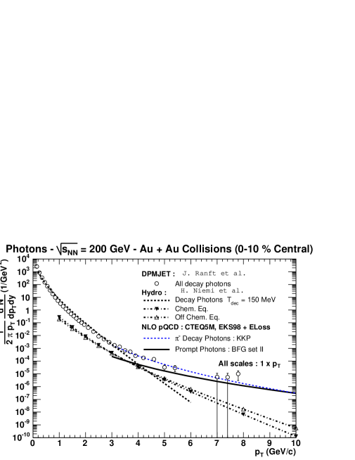
Figure 71: Photon spectra in Au+Au collisions at $\sqrt{s}=200$ GeV. Thermal emission is calculated assuming either full thermal equilibrium in the plasma phase (dashed-dotted line with dark triangle) or a gluon-rich plasma (dashed-dotted lines with open triangle). Decay photons from thermal hadrons (thick dashed line) and decay photons from NLO QCD pions (thin dashed line) are also shown together with the prompt photons (solid line) and decay photons from the Dpmjet calculation (open circles).

At RHIC we see that around $p_{{}_{T}}\sim$ 3.5 to 4 GeV/c the NLO QCD production of prompt photons (solid line) is of the same order of magnitude as the production of thermal photons (dashed-dotted lines) and the decay photons from hadrons as obtained in the hydrodynamic calculation with $\tau_{~{}0}=0.19$ fm/c (thick dashed line). Thermally emitted photons decrease rapidly with $p_{{}_{T}}$ and compared to the prompt QCD photons and photons from hadronic decays they become negligible already around 6 GeV/c. There is no sensitivity to whether or not the plasma is in chemical equilibrium except at the higher values of $p_{{}_{T}}$ where the thermal rate is negligibly small. One can also observe an overall agreement between DPMJET and the NLO QCD + hydrodynamic estimates over the whole $p_{{}_{T}}$ spectrum.

We next discuss the LHC predictions shown in Fig. 72. The prompt NLO QCD photon spectrum is given by the lower solid line and the spectrum of decay photons from $\pi^{0}$’s, produced through NLO QCD jet fragmentation, by the upper solid line. The dotted and dashed lines show the decay photons from all hadrons in the hydrodynamic calculation with $T_{\rm dec}$ either 120 MeV (dotted) or 150 MeV (dashed). Thermal photons are shown both from a calculation when the quark-gluon plasma is assumed to be in full thermal and chemical equilibrium (dashed-dotted line with filled triangles) and when the plasma is dominated by gluons and is not in chemical equilibrium (dashed-dotted line with open triangles). As mentioned before kinetic equilibrium is assumed also in the latter case and in both cases the initial time in the hydrodynamic calculation is $\tau_{0}=0.1$ fm/c. The two sets of predictions cannot be distinguished. Given the same initial energy density from the primary production, the deficit of quarks and antiquarks, which reduces the photon emission, leads to higher values of the temperature which enhance the emission. The slope of thermal production is steeper than for the prompt QCD photons from the interactions of incoming partons but the crossing of thermal and prompt QCD photon spectra takes place at rather high value of $p_{{}_{T}}$ around 6$\ldots$7 GeV/c. However, if the effective thermalization time is longer the crossing region could be as low as $3\ldots 4$ GeV/c.

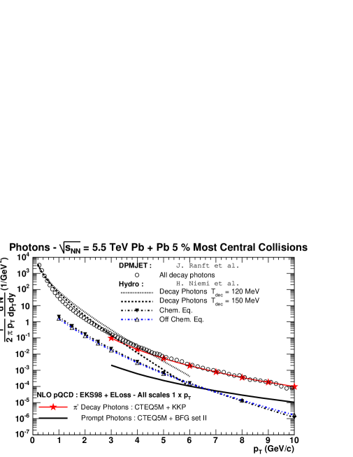
Figure 72: Photon spectra in Pb+Pb collisions at $\sqrt{s}=5.5$ TeV. Thermal emission is calculated assuming either full thermal equilibrium in the plasma phase (dashed-dotted line with dark triangle) or a gluon-rich plasma (dashed-dotted lines with open triangle). Decay photons from thermal hadrons are indicated by dotted or dashed lines depending of the decoupling temperature. The spectrum of NLO prompt and decay photons are shown by the lower and upper solid lines respectively.

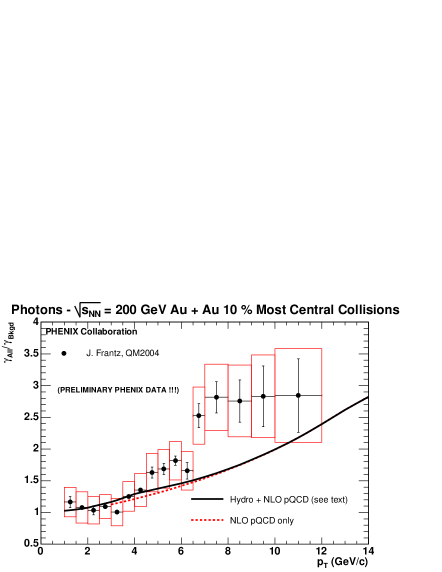
Figure 73: Ratio of all (NLO+Hydro) photons over all decay (NLO QCD + Hydro) photons as a function of $p_{{}_{T}}$, in Au+Au collisions at $\sqrt{s}=$ 200 GeV. Predictions for primary production of prompt photons (NLO QCD) are shown by the dotted line. Preliminary data from PHENIX are also displayed.

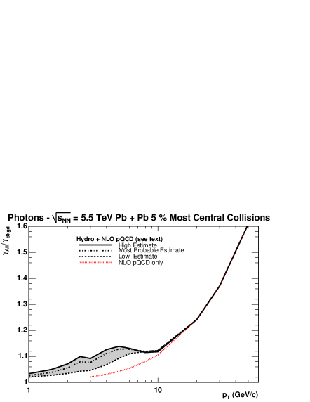
Figure 74: Ratio of all (NLO+Hydro) photons over all decay (NLO QCD + Hydro) photons as a function of $p_{{}_{T}}$, in Pb+Pb collisions at $\sqrt{s}=$ 5.5 TeV. Predictions for primary production of prompt photons (NLO QCD) are shown by the dotted line.

In order to compare more clearly the different sources, we have plotted in Figs. 73 and 74, for RHIC and LHC, respectively, the ratio of the spectrum of “all” photons to the background (from hadronic decays) photon spectrum.

In Au+Au collisions at $\sqrt{s}=$ 200 GeV, the thermal photons from the hydrodynamic calculation (solid line) provide a small increase in the ratio $\gamma_{\rm All}/\gamma_{\rm Bkgd}$ in the range 3 GeV/c to 6 GeV/c compared to a pure pQCD estimate (dotted line). However this increase appears too small to be observed experimentally. The thermal results are insensitive to whether the plasma is in chemical equilibrium or not. With increasing $p_{{}_{T}}$, due to prompt QCD photons, the fraction of direct photons grows quite rapidly reaching 50 % already at 10 GeV/c. Comparison with PHENIX preliminary data [87] shows a good agreement for $p_{{}_{T}}<$ 4 GeV/c (where thermal effects play a major role) while the theoretical predictions tend to underestimate the ratio at larger $p_{{}_{T}}$ values where the NLO QCD production mechanism is dominant. This disagreement can be related to an overestimate, at large $p_{{}_{T}}$, of $\pi^{0}$ rates, and hence of decay photons, compared to data (see Fig. 69).

In Fig. 74 the ratio $\gamma_{\rm All}/\gamma_{\rm Bkgd}$ is shown for Pb+Pb collisions at LHC. The upper curve is obtained by using the prediction from the plasma in equilibrium for the thermal photons and 150 MeV for $T_{\rm dec}$ which, for the calculation of the decay photons, gives the steeper slope for the hadron spectra. In the case of the lower curve off-chemical equilibrium is assumed in calculating the thermal photons and $T_{\rm dec}=120$ MeV in obtaining the hadron spectra for the calculation of the decay photons. The dash-dotted line indicates the prediction obtained under the hypothesis of a gluon rich plasma and a decoupling temperature of 150 MeV consistent with the RHIC data (see Fig. 68). Note also the rather flat dependence, at around the 10 to 15% level, of the ratio for $p_{{}_{T}}$ between 3 and 10 GeV/c where thermal effects play a role. Above 10 GeV/c the ratio increases rapidly with $p_{{}_{T}}$ so that direct photon production represents 25% at $p_{{}_{T}}=20$ GeV/c and 60% at $p_{{}_{T}}=60$ GeV/c.

In conclusion, the overall behaviour of $\gamma_{\rm All}/\gamma_{\rm Bkgd}$ is similar with that in the RHIC results but the ratios differ in details, in particular the enhancement due to thermal production is shifted up to the interval from 3 to 10 GeV/c and is larger.

We should add to the rate of photons produced in A+A collisions also the possibility that before a hard final state parton fragments into a jet of hadrons it may convert to a photon in the parton medium via Compton scattering or annihilation as proposed in  [181]. The resulting spectrum should have a power behavior and could dominate over the thermal photons already for $p_{{}_{T}}\sim 6\ldots 9$ GeV/c (see Fig. 63). This mechanism is hard to quantify, however, and the presently available calculation has been done assuming plasma evolution without transverse expansion which is not compatible with the one used in our discussion. Therefore we do not attempt a quantitative comparison. Nevertheless, it would be important to further develop the modelling of this process.

There are other uncertainties in these results for $\gamma_{\rm All}/\gamma_{\rm Bkgd}$, the most serious for the thermal contribution being the uncertainty in $\tau_{0}$, the initial time in the hydrodynamical calculation when the matter is assumed to reach an (approximate) kinetic equilibrium. If the time for the beginning of the production of thermal photons is more than 1 fm/c, possibilities for observing them are not very encouraging. However, one should not be too discouraged by those estimates which predict kinetic thermalization times over 1 fm/c. It may take time for the initially produced parton system to get equilibrated, but even then we can expect it to be a dense system of interacting partons right after their production. When interacting (and evolving towards equilibrium), these partons would emit photons. The uncertainty then is if the hydrodynamical calculation with the assumption of kinetic equilibration gives a reasonable estimate of the emission of photons from a nonequilibrium but dense parton matter.

If the production of photons from secondary collisions is large enough to be observed, then even if the produced parton system never reaches equilibrium, these photons carry information on the typical scale of relative momenta in the parton matter and on its density. In an equilibrated system the momentum scale is given by the temperature, and the density and the momentum scale are related. If early equilibration does not take place the observation of photons from secondary collisions would still be a direct window into the properties of the densest phase of partonic matter formed in nuclear collisions.

As the discussion above shows, the phenomenology of photon production is far from being on a quantitative basis yet. However, our studies seem to indicate that, at LHC, the ratio of direct photons over decay photons, whatever their origin, should be 10% or more for $p_{{}_{T}}>$ 3 to 4 GeV/c. At the lowest values of $p_{{}_{T}}$ the direct photons would be mostly produced in secondary collisions while around 10 Gev/c they would be of mixed origin with the perturbatively produced (i. e. in primary collisions) photons becoming dominant with increasing $p_{{}_{T}}$. Many of the uncertainties concerning thermal production would be reduced if the model parameters could be fixed from hadron data leaving then the photon spectrum as a crucial consistency check of the whole approach.

7.3 Comparing lepton pair spectra from main sources

In this section we briefly compare lepton pairs from NLO QCD interactions, from hadron decays, and from thermal interactions in the plasma phase. We present the transverse momentum distributions of pairs in the mass interval [0.2,0.6] GeV/c² and consider correlated pairs only. The results, discussed separately for each source in previous sections, are summarized in Fig. 75. In all models and calculations the same input is used as for the photon summary in the previous section.

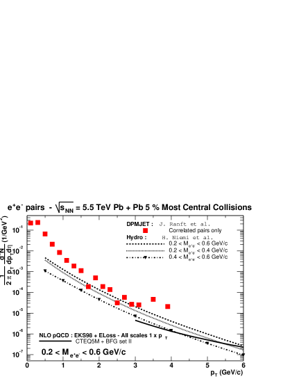
Figure 75: Lepton pairs from thermal emission are compared with those from prompt emission in the NLO QCD approach.

The main background coming from hadron decays is illustrated with DPMJET results (filled squares) since the DMPJET calculation agrees with the NLO QCD results for hadrons at large and with the hydrodynamic calculation at low transverse momentum. Results from the NLO QCD calculation on pair production are shown as the solid line and thermal pairs from the hydrodynamic calculation as a dashed line. Contributions of thermal pairs from each half of the mass interval are shown also separately to draw attention to the rather strong mass dependence in the thermal production.

Statistics of the DPMJET calculation is not large enough for obtaining results beyond $p_{{}_{T}}\sim 3\ldots 4$ GeV/c but the indications of the low–$p_{{}_{T}}$ behaviour seem clear: pairs from hadron decays dominate at low $p_{{}_{T}}$ but they have a steeper $p_{{}_{T}}$ dependence and seem to join the distribution of thermal pairs around $p_{{}_{T}}\sim 3$ GeV/c. Pairs from hard interactions of incoming partons, given by the NLO QCD result, overtake the thermal production around $p_{{}_{T}}\sim 6$ GeV/c. If the $p_{{}_{T}}$ dependence of different contributions is similar to that in the photon production, we would conclude that for $p_{{}_{T}}~{}\raise 1.29167pt\hbox{$>$\kern-7.5pt\raise-4.73611pt\hbox{$\sim$}}~{}3$ GeV/c the background from the hadron decay pairs has the same size as the sum of thermal and NLO QCD pairs and might go below it as $p_{{}_{T}}$ increases.

In summary, considering the signal-to-background ratio the $e^{+}e^{-}$ channel appears at first sight quite promising for the study of hot matter in nucleus-nucleus collisions. However, our discussion is preliminary and lots of work remains to be done in order to confirm if the spectrum of direct lepton pairs can be extracted from the large background of uncorrelated pairs within the statistics which could be expected to be available at LHC.

8 PRODUCTION OF PHOTONS AT “LARGE” TRANSVERSE MOMENTUM AND CORRELATION STUDIES

F. Arleo, P. Aurenche, J.-Ph. Guillet,O.L. Kodolova, I.P. Lokhtin, A. Nikitenko, I.N. Vardanyan, M. Werlen

It was shown in previous chapters that the signal for direct, thermal or non-thermal, photon production in A+A collisions is not too large compared to various backgrounds, making it a challenging but not easy task to use inclusive photon production as a signal for quark-gluon plasma formation in heavy ion collisions. In this chapter we consider correlation observables in a kinematical regime where the photon is produced “promptly” in a hard QCD process and we study the hadrons recoiling from the photon. These hadrons are decay products of a jet, most probably a quark. Since the fragmentation properties of jets are supposed to be modified by medium effects, differences in the shape of the correlations should be seen when comparing $pp$ and A+A collisions. In the next section one looks at the global jet and study, from an experimental (CMS) point of view, the effect of smearing and efficiency on an assumed energy loss. Then a discussion is given on photon-photon and photon-hadron correlations where the hadron or the second photon are decay products of the jet. One takes a more phenomenological point of view and discuss various functions in the hope of determining the correlation most sensitive to medium effects. All studies are preliminary in the sense that they are conducted at the leading order and therefore will be modified by NLO corrections which may be very important in some corners of phase space.

8.1 Photon-jet correlation at CMS

O.L. Kodolova, I.P. Lokhtin, A. Nikitenko, I. Vardanian

Among other proposed signals of jet quenching (see Chapter ”Jets” of this Report [44]), the $p_{{}_{T}}$-imbalance between a produced jet with a gauge boson in $\gamma+$jet [46, 185] and $Z+$jet [186] production has been identified as being observable in heavy ion collisions using the CMS detector [16]. The dominant leading order diagrams for high transverse momentum $\gamma$ + jet production are shown in figure 76. Contrary to the gluon-dominated jet pair production where one could investigate jet quenching due to mostly gluon energy loss in dense matter, $\gamma+$jet channel gives a possibility to study quark energy loss. The main background here is hard jet pair production when one of the jet in an event is misidentified as a photon. The leading $\pi^{0}$ in the jet is a main source of the misidentification. Table 4 presents the event rates for signal and background processes in one month of Pb+Pb beams (a half of the time is supposed to be devoted to data taking), $R=1.2\times 10^{6}$ s, assuming luminosity $L=5\times 10^{26}~{}$cm^-2s^-1 to that

$$N(events)=R\sigma^{h}_{AA}L,$$

where production cross sections in minimum bias nucleus-nucleus collisions is obtained from those in $pp$ interactions at the same energy ($\sqrt{s}=5.5$ TeV) using simple parameterization $\sigma^{h}_{AA}=A^{2}\sigma^{h}_{pp}$. The cross section in $pp$ collisions were evaluated using the PYTHIA_$6.1$ Monte-Carlo generator [62] with the CTEQ5L parton distribution function. Note that the influence of nuclear shadowing is practically negligible for the region of sufficiently hard $\gamma+$jet production, $x_{1,2}\sim\sqrt{\widehat{s}/s}\mathrel{\mathchoice{\lower 3.6pt\vbox{\halign{$\mathsurround=0pt\displaystyle\hfil#\hfil$\cr>\crcr\sim\crcr}}}{\lower 3.6pt\vbox{\halign{$\mathsurround=0pt\textstyle\hfil#\hfil$\cr>\crcr\sim\crcr}}}{\lower 3.6pt\vbox{\halign{$\mathsurround=0pt\scriptstyle\hfil#\hfil$\cr>\crcr\sim\crcr}}}{\lower 3.6pt\vbox{\halign{$\mathsurround=0pt\scriptscriptstyle\hfil#\hfil$\cr>\crcr\sim\crcr}}}}0.2$. However, large theoretical uncertainties in absolute rates in $pp$ collisions come from choice of the parton distribution functions, next-to-leading corrections, etc. It means that measurements in $pp$ or D+D collisions at the same or similar energies per nucleon as in the heavy ion runs are strongly desirable to determine the baseline rate precisely.

Table 4: Expected rates for $\gamma$+jet and $\pi_{0}(\rightarrow 2\gamma)$+jet channels in one month of Pb$-$Pb beams.

Channel	Barrel, $|\eta|<1.5$	Barrel+Endcap $|\eta|<3$
$\gamma$+jet, $E_{T}^{jet,\gamma}>100$ GeV	1.6$\times$103	3.0$\times$103
$\pi_{0}(\rightarrow 2\gamma)$+jet, $E_{T}^{jet,\gamma}>100$ GeV	8.4$\times$103	2.2$\times$104

One can see that even for events with $E_{T}>100$ GeV the background is still dominant. Signal-to-background ratio becames close to $1$ only above $200$ GeV. The identification of the influence of the dense medium formation on signal spectra requires the reduction of the background. One of the possibilities is to apply some kind of the photon isolation, so called ”zero suppression criteria”, which requires no energy above a given threshold around photon (see section ”Photon detection at CMS” for details). In this case the signal-to-background ratio at $E_{T}>100$ GeV can be improved by a factor about 2.3 at the cost of a $14\%$ reduction of the signal. Another possibility is to apply some kinematical cuts, which do not have influence on the $p_{{}_{T}}$-imbalance of the process (i.e. not result in shift of maximal value of $E_{T}^{\gamma}-E_{T}^{jet}$ distribution).

The possibility to observe the medium-induced energy loss of quark-initiated jet using photon-jet correlation in heavy ion collisions with CMS detector has been investigated in [187, 16]. It has been found that initial state gluon radiation and finite jet energy resolution (which is much larger than photon energy resolution) result in significant smearing of distribution of differences in transverse energies between the photon and jet. But it is still symmetric: $E_{T}^{\gamma}=E_{T}^{jet}$ only in average (not for each given event). The non-symmetric shape of the distribution appears if a jet loses energy: the maximal value of the distribution is equal to the average energy loss of the quark-initiated jet at the given energy detection threshold, $E_{T}^{jet}\sim 100$ GeV in CMS case. Note that we are not measuring energy loss of a leading quark by such a way, but getting total loss of quark-initiated jet outside the given jet cone.

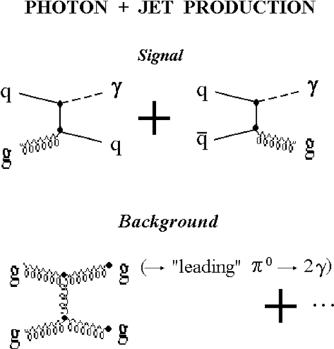
Figure 76: Leading order diagrams for $\gamma$+jet (signal) and $\pi_{0}(\rightarrow 2\gamma)$+jet (background) production.

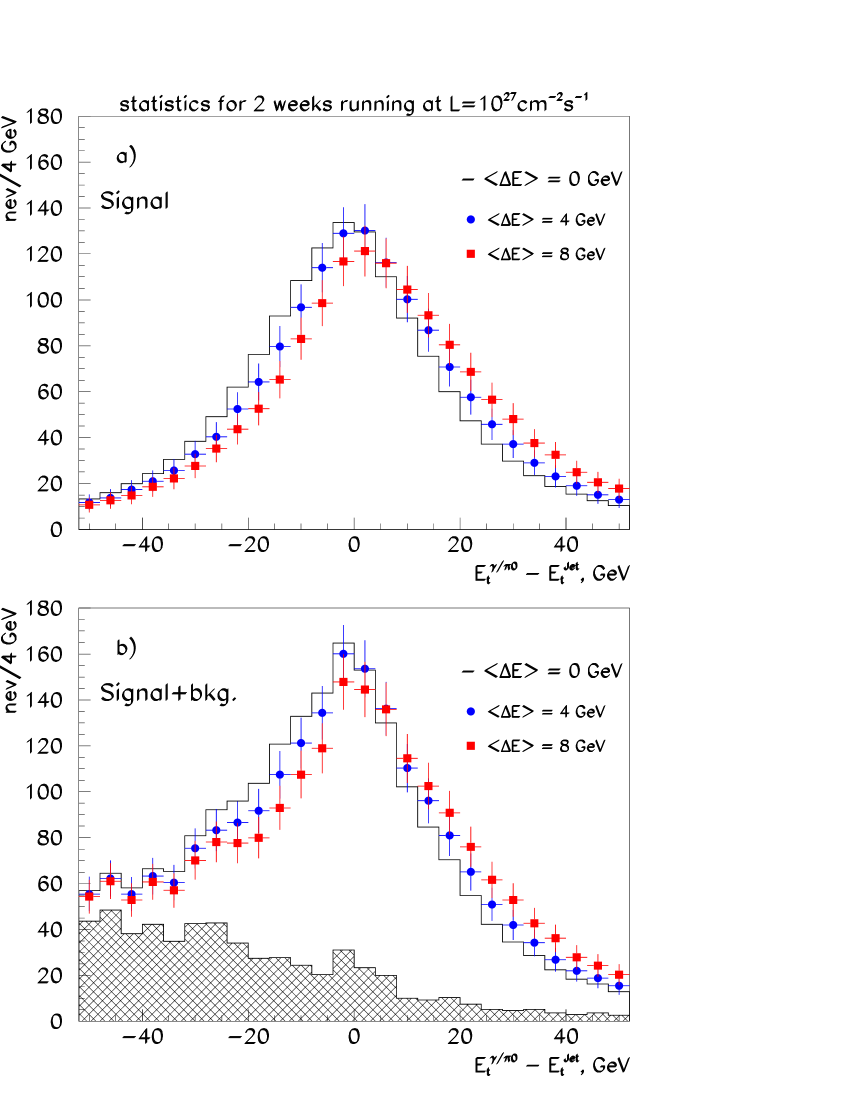
Figure 77: The distributions of differences in transverse energy between the $\gamma$ and jet with $E_{t}^{\gamma,~{}jet}>120$ GeV: a) without ($\pi^{0}$ + jet) background, b) with ($\pi^{0}$ + jet) background. The pseudorapidity coverage is $\mid\eta_{\gamma,~{}jet}\mid<1.5$. Different values of jet in-medium energy loss, initial state gluon radiation and finite jet energy resolution are taken into account.

In order to test the sensitivity of $\gamma$+jet production to jet quenching, it was considered three scenarios with average collisional energy loss of a jet: $<\Delta E_{q}>\simeq 0$, $4$ and $8$ GeV respectively ($<\Delta E_{g}>=9/4\cdot<\Delta E_{q}>$). The jet energy resolution at mid-rapidity obtained for Pb+Pb collisions has also been used to smear the energy of the recoiling parton, as well as the jet rejection factor and signal efficiency [187]. Figure 77 shows the distributions of differences in transverse energy between the photon and jet with $E_{T}^{\gamma,~{}jet}>120$ GeV in one month of Pb+Pb beams without and with ($\pi^{0}$ + jet) background in the pseudorapidity region $\mid\eta^{\gamma,~{}jet}\mid<1.5$ for different values of jet energy loss. In this case a luminosity $L=10^{27}~{}$cm^-2s^-1 was assumed and PYTHIA_$5.7$ version with the default CTEQ2L pdf choice was used. The jet energy resolution leads to a difference between the input values $<\Delta E_{q}>$ and the ones obtained from the spectra. The background of $\pi^{0}$-contamination results in non-zero negative values of the final distributions (figure  77b) already in the case without jet energy loss. However one can see that the shape of the distribution is well distinguished for the scenarios considered. For the region of $(E_{T}^{\gamma}-E_{T}^{jet})>0$ there is a difference for almost every bin greater than $1$ standard deviation for the rather small jet energy loss $8$ GeV and even for the loss $4$ GeV. In the real experiment it would be possible to estimate the number of background events using the region without the signal ($E_{T}^{\gamma}-E_{T}^{jet})<-100$ GeV/c and background shape from Monte-Carlo simulation and/or from $pp$ data. A significant difference in the shape of the $E_{T}^{\gamma}-E_{T}^{jet}$ distribution can allow to optimize extraction of the signal from the experimental spectra.

8.2 Photon-hadron and photon-photon correlations in $pp$ and A+A collisions

F. Arleo, P. Aurenche, J.-Ph. Guillet

In the previous chapters it was suggested that thermal production of photons could be seen for rather low $p_{{}_{T}}$ values. In the following we consider, on the contrary, the case of a photon with a high enough $p_{{}_{T}}$ so that it is produced promptly in a hard QCD process and therefore not affected by thermal effects and we study the decay products of the jet recoiling from this photon. The analogue of the inclusive spectrum Eq. (3), at the leading logarithmic order, can be written [189]

$${d\sigma^{{}^{AB\rightarrow CD}}\over dp_{{}_{T}{{}_{3}}}dy_{3}dp_{{}_{T}{{}_{4}}}dy_{4}}={1\over 8\pi s^{2}} \sum_{a,b,c,d} \int_{z_{3_{min}}}^{1}{dz_{3}\over z_{3}}\ D_{C/c}(z_{3},M_{{}_{F}})\ \int_{z_{4_{min}}}^{1}{dz_{4}\over z_{4}}\ D_{D/d}(z_{4},M_{{}_{F}})\ k_{{}_{T}{{}_{3}}}$$ (64)

$$\delta(k_{{}_{T}{{}_{3}}}-k_{{}_{T}{{}_{4}}})\ {F_{{}_{a/A}}(x_{1},M)\over x_{1}}\ {F_{{}_{b/B}}(x_{2},M)\over x_{2}}\ \ |{\overline{M}}|^{2}_{ab\rightarrow cd}$$

where the $p_{{}_{T}{{}_{i}}}$ (resp. $k_{{}_{T}{{}_{i}}}$) are the final state particle (resp. partonic) transverse momenta and the scaling variables $z_{i}$ are defined by $z_{i}=p_{{}_{T}{{}_{i}}}/k_{{}_{T}{{}_{i}}}$. The quantity $|{\overline{M}}|^{2}_{ab\rightarrow cd}$ is the matrix element squared, averaged over spin and color, of the partonic sub-process $ab\rightarrow cd$. Higher order corrections to Eq. (64) have been calculated [189] and, based on existing data [190, 191, 192], extensive NLO phenomenological studies of correlations have been carried from fixed target energies to the LHC [83, 193]. If one looks at a photon at large enough $p_{{}_{T}{{}_{3}}}$, it will be directly produced and the corresponding fragmentation will reduce to $\delta(1-z_{~{}3})$. Studying various correlation variables will then allow the mapping of the fragmentation function $D_{D/d}(z_{4},M_{{}_{F}})$ since all other ingredients (structure functions, matrix elements) are known. One could then observe the effect of partonic energy loss in the medium by comparing correlation functions in A+A collisions with the equivalent ones in $pp$ collisions. In the following we restrict ourselves to the case of promptly produced photon and do not impose isolation cuts. We do not consider the “background” contribution generated by photons decaying from hadronic resonances, a problem presently under investigation [194].

Figure 78: Comparison of partonic fragmentation functions in the vacuum and in the medium for typical values of the energy loss parameter $\omega_{c}$. Top two figures: $k_{{}_{Td}}=$ 20 GeV/c up quark and gluon into a photon; bottom two figures: $k_{{}_{Td}}=$ 20 GeV/c up quark and gluon into a charged hadron.

How to express final state interactions through medium-modified fragmentation functions remains however far from being clear. To illustrate the effect of parton energy loss in dense media on correlation functions, we shall adopt here the effective model suggested in Ref. [185]. Within this approach, the parton energy shift leads to a rescaling of the momentum fraction $z_{d}$ in presence of a QCD medium,

$$z_{d}=\frac{p_{{}_{Td}}}{k_{{}_{Td}}}\qquad\to\qquad z_{d}^{*}=\frac{p_{{}_{Td}}}{k_{{}_{Td}}-\epsilon}=\frac{z_{d}}{1-\epsilon/k_{{}_{Td}}},$$ (65)

where $p_{{}_{Td}}$ (respectively, $k_{{}_{Td}}$) stands for the transverse momentum of the photon or hadron (respectively, the parton), and $\epsilon$ the energy lost by the hard parton while going through the medium. Consequently, the medium-modified fragmentation functions $D_{D/d}^{med}(z_{d},Q^{2},k_{{}_{Td}})$ may simply be expressed as a function of the standard (vacuum) fragmentation functions $D_{D/d}(z_{d},Q^{2})$ through [185]

$$z_{d}\,D_{D/d}^{med}(z_{d},Q^{2},k_{{}_{Td}})=\int_{0}^{k_{{}_{Td}}-p_{{}_{Td}}}\,d\epsilon\,\,{\cal D}(\epsilon,k_{{}_{Td}})\,\,\,z_{d}^{*}\,D_{D/d}(z_{d}^{*},Q^{2}).$$ (66)

Here, ${\cal D}(\epsilon,k_{{}_{Td}})$ denotes the probability for a parton with transverse energy $E=k_{{}_{Td}}$ to lose an energy $\epsilon$ [188]. Note that medium-induced fragmentation functions now depend explicitely on the parton transverse energy $k_{{}_{T}}$. Assuming the soft gluons radiated by the leading hard parton to be emitted independently, this probability distribution (or quenching weight) can easily be related to the medium-induced gluon spectrum determined perturbatively, $dI/d\omega$, characterized by the energy scale [45]

$$\omega_{c}=\frac{1}{2}\,\hat{q}\,L^{2}$$ (67)

The gluon transport coefficient $\hat{q}$ reflects the medium gluon density while $L$ is the length of matter covered by the hard parton. Note that $\hat{q}$ can be very large in practice in a hot pion gas or quark gluon plasma [195]. Based on the estimate from the pion inclusive spectrum in A+A collisions at RHIC ($\sqrt{s}=200$ GeV), we shall illustrate our results using the following values $\omega_{~{}c}=30$ and $50$ GeV for the characteristic scale of the dense medium produced in nuclear collisions at the LHC. The distribution ${\cal D}(\epsilon,k_{{}_{Td}})$ has been given a simple analytic parameterization in [49] which we shall use in the present calculations.

Since fragmentation functions fall steeply with $z$, even a small shift $\Delta z_{d}=z_{d}^{*}-z_{d}\approx z_{d}\,\epsilon/k_{{}_{Td}}$ in (65) may substantially affect fragmentation processes in presence of a hot and dense QCD medium. This can be seen for instance in Figure 78 where fragmentation functions into a photon (top) or a charged hadron (bottom) are computed for $k_{{}_{T}}=20$ GeV/c up quark (left) and gluon (right) traversing the medium. In particular, we expect the effects of parton energy loss to be more pronounced as $z$ gets larger. This will be further discussed below when correlation functions in nuclear collisions are computed perturbatively.

As an example we consider the following kinematical constraints. Both observed particles (photon or charged hadron) are required to be in a rapidity interval [$-0.5,+0.5$] and furthermore one photon should have a transverse momentum greater than 10 GeV/c while the other photon or the charged hadron is required to have $p_{{}_{T}}>3$ GeV/c. Integrated over all kinematical variables, with the above constraints, we display in Fig. 79 the photon spectrum $d\sigma/d{p_{{}_{T}}}$ for the case of two photon events (left) and the charged hadron spectrum for the photon + hadron events (right). The various dynamical components are shown. In the two photon case they are the “direct” (both photons produced in the hard sub-process), the “one-f” (one photon produced directly and the other by bremsstrahlung from a fragmenting parton) and the “two-f” (both photons produced by bremsstrahlung of the final state partons) .

Figure 79: Details of the various dynamical components in $pp$ collisions at $\sqrt{s}=5.5$ TeV. Left: the photon spectrum in the two photon events; right: the charged hadron spectrum in the photon-hadron events.

The interpretation of the photon-photon figure is easy. For $p_{{}_{T}}<10$ GeV/c, the observed photon is the less energetic of the two photons because of the 10 GeV/c cut imposed on the other photon: the observed photon can only be produced by bremsstrahlung and the figure shows that the “one-f” process dominates by far. When $p_{{}_{T}}>10$ GeV/c, the direct component comes into play but again the “one-f” process is the largest. This confirms that, with the cuts used, the cross section Eq. (64) for the case of two photon production is mainly sensitive to one fragmentation function. For the photon-hadron case the “one-f” (the photon produced directly and the hadron a fragment of a jet) and the “two-f” (both particle fragments of jets) processes are comparable. A word of caution is necessary: as usual in perturbative QCD, the distinction between direct, one-f and two-f is only indicative as the relative weights of the components depends on the choice of the (factorization, renormalization) scales, chosen in this discussion to be all equal to $p_{{}_{T}}$.

In the following we define various correlation functions in $\gamma-\gamma$ events [196] (see Fig. 80) and study their modifications as a function of the assumed energy loss characterized by the value of the parameter $\omega_{c}$. They are :
– the photon $p_{{}_{T}}$ distribution;
– the diphoton invariant mass $m_{\gamma\gamma}$ spectrum;
– the spectrum in the transverse momentum of the pair defined as ${{\tenimbf q}_{{}_{T}}}={{\tenimbf p}_{{}_{T3}}}+{{\tenimbf p}_{{}_{T4}}}$;
– the distribution in the scaled momentum fraction $z_{~{}34}=-{\tenimbf p}_{{}_{T3}}\cdot{\tenimbf p}_{{}_{T4}}/{\tenimbf p}^{2}_{{}_{T3}}$.

Figure 80: Photon-photon correlation functions in Pb+Pb collisions at $\sqrt{s}=$ 5.5 TeV.

Considering the spectrum $d\sigma/dp_{{}_{T}}$ in Fig. 80 one sees that the curve below $p_{{}_{T}}=10$ GeV/c decreases when $\omega_{c}$ increases (energy loss increases), very similarly to the fragmentation functions in Fig. 78. The relative suppression is larger as $p_{{}_{T}}$ increases corresponding to an increase of the effective fragmentation variable $z$. For $p_{{}_{T}}$ above the cut, on the contrary, the medium and the vacuum spectra come closer together when the transverse momentum increases. This can be understood as follows: the detected photon with large momentum is produced directly while the other photon is produced predominantly near the 3 GeV/c threshold and its effective $z\sim z_{~{}34}$ decreases when the $p_{{}_{T}}$ of the directly produced photon increases: since at small $z$ the energy loss in the medium is small (see Fig. 78) the in-medium curve and the “vacuum” curve approach each other.

The di-photon invariant mass spectrum (upper right plot in Fig. 80) shows, in vacuum as well as in the medium, a characteristic bump above $m_{\gamma\gamma}=$ 20 GeV/c due to the onset of the “direct” production mechanism. Only “one-f” and “two-f” processes contribute below this threshold. When increasing the energy loss, these last two processes are suppressed, leading to a larger suppression of the invariant mass distribution at low masses and an increasingly marked shoulder since the direct channel is not affected by the medium.

Figure 81: Ratio of photon-photon correlation functions in Pb+Pb collisions and $pp$ collisions at $\sqrt{s}=$ 5.5 TeV.

The peaked shape of the transverse momentum distribution of the pair (lower left plot in Fig. 80) at $p_{{}_{T}}\sim$ 7 GeV/c is an effect of the imposed asymmetric lower cuts on the photon momenta and the decrease of the spectrum at the lower $q_{{}_{T}}$ values when the energy loss increases is easy to understand: to obtain a small $q_{{}_{T}}$ value both photons should have similar $p_{{}_{T}}$ which means that the bremsstrahlung photon will be emitted from a parton with a large $z$ value, a configuration highly unfavored in the medium. The suppression of the spectrum for small $q_{{}_{T}}=0$ will be somewhat modified by higher order corrections which will smear the direct process contribution shown, in the figure, by a point at $q_{{}_{T}}=0$. On the other hand at large $q_{{}_{T}}$ no dramatic medium effect is expected since the dominant kinematics will be a photon (directly produced) at large $p_{{}_{T}}$ and a bremsstrahlung photon at very small $p_{{}_{T}}$, equivalently small $z$, both of which are not affected by medium effects

Finally, the distribution in the scaling variable $z_{~{}34}$ (bottom right plot) nicely reflects the behavior of the fragmentation function when medium effects are increasing: the scaling variable and the fragmentation variable $z$ are very closely related and it is natural that the $z_{~{}34}$ be reminiscent of the behavior of the fragmentation functions shown in Fig. 78 when the energy loss increases.

Figure 82: Photon-charged hadron correlation functions in Pb+Pb collisions at $\sqrt{s}=$ 5.5 TeV.

The energy loss features of the observables we just discussed are emphasized if we plot the ratio of the correlation functions in A+A collisions over the same in $pp$ collisions. This is done in Fig. 81. The effect of the energy loss does not reduce simply to a change of normalisation of the correlations but also to a change of shape. For the normalized $d\sigma/dp_{{}_{T}}$ distribution (top left) one recognizes the increase in the suppression as $p_{{}_{T}}$ increases below the threshold value of 10 GeV/c, corresponding to an increasing $z$ value of the detected photon while above $p_{{}_{T}}=$ 10 GeV/c the effect of the energy loss is, as expected, becoming less and less visible. Particularly interesting are also the normalized $d\sigma/dq_{{}_{~{}T}}$ (bottom left) and $d\sigma/dz_{34}$ (bottom right) correlations which display a marked dependence on the variable $q_{{}_{~{}T}}$ and $z_{34}$ respectively.

All these studies have been carried out in the LO approximation. Clearly, higher order corrections will somewhat smear the results specially near thresholds or infra-red singular points ($z=1$ or ${\boldsymbol{q}}_{{}_{~{}T}}=0$ for example). Very preliminary studies in the NLO approximation, assuming that higher order corrections can be calculated in the same way in $pp$ and in A+A collisions, show that the effects of the energy loss can still be clearly seen in the correlation functions [194].

As a further illustration of correlation studies we present in Fig. 82 the results for photon-charged hadron observables, with the same kinematical constraints as before: $p_{{}_{T}}>$ 10 GeV/c for the photon and $p_{{}_{T}}>$ 3 GeV/c for the hadron. The interpretation of the curves is very similar to the case of photon-photon correlations the main advantage of the photon-hadron channel being a much higher counting rate.

9 OUT-OF-EQUILIBRIUM PHOTON PRODUCTION

I. Dadić, F. Gelis, G.D. Moore, J. Serreau

In the previous sections, 6 and 7, the rate of thermal photon production in the quark-gluon plasma is calculated ignoring the finite life time of the plasma. Recently however it has been argued that finite life-time effects could considerably increase the rate of production. We discuss this class of models and show that they are based on an unrealistic modeling of the initial and final state conditions which leads to an infinite amount of energy being radiated away by the photons. These models are therefore unphysical. A possible approach to non-equilibrium aspects is then briefly sketched.

9.1 Transient effects in the real-time approach

I. Dadić, F. Gelis, G.D. Moore

In equilibrium, one usually defines the initial density operator at an initial time $t_{i}$ which is infinitely remote in the past. However, one may wonder if any changes are to be expected when the initial state is defined at some finite time $t_{i}$. Some recent papers by Wang, Boyanovsky and Ng [197, 198] suggested that one can see transient effects in the photon radiation of a thermal system that exists only for a finite amount of time. A similar model has been considered by Dadić, based on [199, 200, 201], but there are no published results on photon production at the time of writing this report. The main feature of the photon emission spectrum obtained in [197, 198] is that it decreases as a power of the photon energy instead of the usual exponential spectrum. This implies that already at moderate photon energies, the prediction of [197, 198] dominates by several orders of magnitude over the usual thermal rates.

We start this section by discussing some general properties of an equilibrated system prepared at a finite initial time, and discuss what to expect if the particles in the initial bath are non interacting. We proceed with a derivation of the results of [197, 198] for the photon emission rate in such a model, and we discuss also briefly the approach of [199, 200, 201]. Finally, we close the section by discussing the fact that this model leads to infinite “vacuum” contributions, precluding any phenomenological application of these rates.

9.1.1 Starting the equilibrium evolution at a finite time

Let us first assume that the density operator at $t_{i}$ is $\rho(t_{i})=\exp(-\beta H)$, where $H$ is the full Hamiltonian, including all the interactions. In order to calculate perturbatively a correlator like $\left<{\rm T}\phi(x_{1})\cdots\phi(x_{n})\right>$ where $\left<A\right>\equiv{\rm Tr}\,(\rho(t_{i})A)/{\rm Tr}\,(\rho(t_{i}))$, one has to extract the two sources of dependence on the coupling constants. The first one is the usual dependence of the Heisenberg field $\phi(x)$ on the coupling constants, and it is readily extracted by going to the interaction picture:

$$\phi(x)=U(t_{i},x_{0})\phi_{{}_{I}}(x)U(x_{0},t_{i})\;,$$ (68)

where $U$ is an evolution operator defined as

$$U(t_{2},t_{1})={\rm P}\,\exp i\int_{t_{1}}^{t_{2}}d^{4}x{\cal L}_{\rm int}(\phi_{{}_{I}}(x))$$ (69)

with ${\cal L}_{\rm int}$ the part of the Lagrangian density that contains the interactions and $\phi_{{}_{I}}$ a free field that coincides with the Heisenberg field at $x_{0}=t_{i}$.

However, there is a second source of dependence on the coupling constants, which is present in the density operator itself [202, 203]. This can be extracted thanks to the following formula that relates the full density operator to the one defined with the non-interacting Hamiltonian $H_{0}$ [204]:

$$e^{-\beta H}=e^{-\beta H_{0}}{\rm P}\,\exp i\int_{t_{i}}^{t_{i}-i\beta}d^{4}x{\cal L}_{\rm int}(\phi_{{}_{I}}(x))\;.$$ (70)

Eqs. (68), (69) and (70) explain the structure of the time integration contour in the real-time formalism [205, 206, 207, 208, 209]: it starts on the real axis at $t_{i}$ and goes along the real axis up to some final time $t_{f}$ (which can be $+\infty$, but needs in fact only to be larger than any physical time in the problem, since causality forbids any dependence of physical quantities upon this time), then goes back to $t_{i}$ along the real axis, and finally goes down to $t_{i}-i\beta$ following a segment parallel to the imaginary axis.

The bare propagators in this formalism obey the so-called Kubo-Martin-Schwinger (KMS) symmetry [210, 211], which reads

$$G_{0}(t_{i},y_{0})=\alpha G_{0}(t_{i}-i\beta,y_{0})\;,$$ (71)

where $\alpha=1$ for a real scalar field, $\alpha=\exp(\beta\mu q)$ for a boson that carries the conserved charge $q$ with an associated chemical potential $\mu$, and $\alpha=-\exp(\beta\mu q)$ for a fermion carrying the conserved charge $q$. The same symmetry holds for the second point of the propagator, with $q$ changed into $-q$. Because the number of fermion lines arriving at a vertex is even and because the total conserved charge arriving at a vertex is zero, it is easy to verify that any Feynman diagram made of these bare propagators and where the time integrations at the vertices run on the previously defined contour is independent of the initial time $t_{i}$ [202, 212]. A corollary of this property is that all the Feynman diagrams depend only on differences of their external times, even if they have been calculated on a contour that breaks invariance under time translation because of the finite $t_{i}$.

Physically, this result means the following: if one prepares a system in a state of thermal equilibrium at some finite time $t_{i}$, all the Green’s functions of the theory are independent of $t_{i}$ and there is no way to tell what the initial time was. In other words, there are no observable transient effects in a system initially prepared in a state of thermal equilibrium (provided the particles are interacting in the initial statistical ensemble).

9.1.2 Non interacting initial statistical ensemble

In the previous argument, the contribution of the vertical branch of the contour is crucial in order to achieve a result that does not depend on $t_{i}$. Indeed, the KMS symmetry that relates the values of the propagators at both ends of the contour is of no help if we terminate the contour at $t_{i}$. If we perform the time integrations at the vertices using only the two horizontal branches of the contour (i.e. the so-called Keldysh contour), then we lose the property of independence on $t_{i}$, as well as the invariance under time translations of the Green’s functions, and there are now transient effects.

Given that the vertical branch of the time path arises from Eq. (70), not using the vertical part is equivalent to using an initial density operator $\rho(t_{i})=\exp(-\beta H_{0})$ which does not contain the interaction terms of the Hamiltonian. In other words, this is equivalent to having initially a statistical ensemble of non interacting particles. An identical situation would be the following: start at $t=-\infty$ with the density operator $\rho(-\infty)=\exp(-\beta H_{0})$ and assume that all the coupling constants are zero before $t_{i}$ and jump to their normal value at $t_{i}$. Indeed, if we start with $\rho(-\infty)=\exp(-\beta H_{0})$ and if we have a non interacting dynamics between $-\infty$ and $t_{i}$, then we will have $\rho(t)=\exp(-\beta H_{0})$ as long as the interactions remain zero, by virtue of $\dot{\rho}(t)=-i[H_{0},\rho(t)]=0$.

9.1.3 Photon production

Let us now describe how one could calculate the production of photons when the initial ensemble is a non-interacting statistical ensemble. This system is implemented by taking $\rho(t_{i})=\exp(-\beta H_{0})$, with a time path that has only the two horizontal branches.

Derivation of the results of [197, 198]

The phase-space density of photons at time $t$ in the system is given by:

$$2p_{0}\frac{dN_{\gamma}}{d^{3}{\boldsymbol{x}}d^{3}{\boldsymbol{p}}}=\frac{1}{(2\pi)^{3}}\frac{1}{V}\sum_{{\rm pol\ }\lambda}\;{\rm Tr}\left(\rho(t)a^{\dagger}_{\lambda}({\boldsymbol{p}})a_{\lambda}({\boldsymbol{p}})\right)=\frac{1}{(2\pi)^{3}}\frac{1}{V}\sum_{{\rm pol\ }\lambda}\;{\rm Tr}\left(\rho(t_{i})a^{\dagger}_{\lambda}(t,{\boldsymbol{p}})a_{\lambda}(t,{\boldsymbol{p}})\right)\;,$$ (72)

where $\rho(t)$ is the time-dependent density operator, $a^{\dagger}_{\lambda}({\boldsymbol{p}})$ is the photon creation operator in the Schrödinger picture and $V$ is the volume of the system. In the second equality, we use the cyclicity of the trace in order to transpose the time dependence from the density operator into the number operator, and we have defined:

$$a_{\lambda}(t,{\boldsymbol{p}})\equiv e^{iH(t-t_{i})}a_{\lambda}({\boldsymbol{p}})e^{-iH(t-t_{i})}\;.$$ (73)

This time-dependent creation operator is related to the Heisenberg field via:

$$a^{\dagger}_{\lambda}(t,{\boldsymbol{p}})=-i\int d^{3}{\boldsymbol{x}}\;e^{-ip\cdot x}\stackrel{{\scriptstyle\leftrightarrow}}{{\partial}}_{x_{0}}A^{\mu}(x)\epsilon_{\mu}^{\lambda}({\boldsymbol{p}})\;,$$ (74)

where $\epsilon_{\mu}^{\lambda}({\boldsymbol{p}})$ is the appropriate polarization vector. Inserting Eq. (74) in Eq. (72), taking the time derivative, and using the equation of motion of the Heisenberg fields, we obtain:

$$2p_{0}\frac{dN_{\gamma}}{d^{4}xd^{3}{\boldsymbol{p}}} =\frac{1}{(2\pi)^{3}}\frac{1}{V}\sum_{{\rm pol\ }\lambda}\epsilon_{\mu}^{\lambda*}({\boldsymbol{p}})\epsilon_{\nu}^{\lambda}({\boldsymbol{p}})\lim_{y_{0}\to x_{0}} e\,{\rm Tr}\Big{(}\rho(t_{i})\big{[}J^{\mu}(x_{0},{\boldsymbol{p}})(\partial_{y_{0}}-ip_{0})A^{\nu}(y_{0},{\boldsymbol{p}})$$ (75)

$$+(\partial_{y_{0}}+ip_{0})A^{\nu}(y_{0},{\boldsymbol{p}})J^{\mu}(x_{0},{\boldsymbol{p}})\big{]}\Big{)}\;,$$

where $J^{\mu}(x_{0},{\boldsymbol{p}})$ is the spatial Fourier transform of the current $\overline{\psi}(x)\gamma^{\mu}\psi(x)$ ($\psi$ is the Heisenberg fermionic field). One can also write $J^{\mu}(x_{0},{\boldsymbol{p}})A^{\nu}(y_{0},{\boldsymbol{p}})={\rm P}\,J^{\mu}_{-}(x_{0},{\boldsymbol{p}})A^{\nu}_{+}(y_{0},{\boldsymbol{p}})$, where ${\rm P}$ denotes the path ordering along the Keldysh contour, and the indices $\pm$ indicate on what branch of the contour a field is kept. At this point, one can expand the Heisenberg fields in terms of the free fields of the interaction picture. Since ${\rm Tr}\,(\rho(t_{i})A^{\nu}_{\rm in})=0$, one must at least expand one order further in the electromagnetic coupling $e$. Truncating the expansion at the first non-zero order in $e$, but keeping all orders in the strong interactions, we obtain the following formula

$$2p_{0}\frac{dN_{\gamma}}{d^{4}xd^{3}{\boldsymbol{p}}}=\frac{1}{(2\pi)^{3}}\frac{1}{V}\sum_{{\rm pol\ }\lambda}\epsilon_{\mu}^{\lambda*}({\boldsymbol{p}})\epsilon_{\nu}^{\lambda}({\boldsymbol{p}})\lim_{y_{0}\to x_{0}}e^{2}\int_{\cal C}dz_{0}\int\frac{d^{3}{\boldsymbol{k}}}{(2\pi)^{3}}$$

$$\!\!\!\!\!\!\!\!\!\!\!\!\times\,\Big{[}(\partial_{y_{0}}-ip_{0})\left<{\rm P}\;A^{\nu}_{\rm in,+}(y_{0},{\boldsymbol{p}})A^{\alpha}_{\rm in}(z_{0},{\boldsymbol{k}})\right>\left<{\rm P}\;J^{\mu}_{\rm in,-}(x_{0},{\boldsymbol{p}})J_{\alpha}{}_{\rm in}(z_{0},{\boldsymbol{k}})e^{i\int_{\cal C}{\cal L}_{\rm int}^{QCD}}\right>$$

$$\!\!\!\!\!\!\!\!\!\!+(\partial_{y_{0}}+ip_{0})\left<{\rm P}\;A^{\nu}_{\rm in,-}(y_{0},{\boldsymbol{p}})A^{\alpha}_{\rm in}(z_{0},{\boldsymbol{k}})\right>\left<{\rm P}\;J^{\mu}_{\rm in,+}(x_{0},{\boldsymbol{p}})J_{\alpha}{}_{\rm in}(z_{0},{\boldsymbol{k}})e^{i\int_{\cal C}{\cal L}_{\rm int}^{QCD}}\right>\Big{]}\;,$$ (76)

where ${\cal L}_{\rm int}^{QCD}$ is the QCD part of the interactions, and where ${\cal C}$ is the Keldysh contour that runs from $t_{i}$ to $+\infty$ and then back to $t_{i}$. $\left<\cdots\right>$ denotes the average over the initial ensemble, and we have used the fact that we can factorize the photon fields and the quark fields because the initial density operator does not couple photons and quarks. The first of these correlators contains a factor $(2\pi)^{3}\delta({\boldsymbol{p}}+{\boldsymbol{k}})$ which is used to integrate out the vector ${\boldsymbol{k}}$. Then the second correlator brings a factor $(2\pi)^{3}\delta(0)$ which should be interpreted as the volume of the system, and cancels the factor $1/V$. At this point, it is a simple matter of algebra to work out the derivatives of the photon-photon correlator, and we get:

$$2p_{0}\frac{dN_{\gamma}}{d^{4}xd^{3}{\boldsymbol{p}}}=\frac{e^{2}}{(2\pi)^{3}}\sum_{{\rm pol\ }\lambda}\epsilon_{\mu}^{\lambda*}({\boldsymbol{p}})\epsilon_{\nu}^{\lambda}({\boldsymbol{p}})\int_{-\infty}^{+\infty}\frac{d\omega}{\pi}\frac{\sin((p_{0}-\omega)(x_{0}-t_{i}))}{p_{0}-\omega}$$

$$\qquad\qquad\qquad\qquad\times\Big{[}(1+n_{\gamma}^{0}(p_{0}))\Pi_{+-}^{\mu\nu}(\omega,{\boldsymbol{p}})-n_{\gamma}^{0}(p_{0})\Pi_{-+}^{\mu\nu}(\omega,{\boldsymbol{p}})\Big{]}\;,$$ (77)

where $n_{\gamma}^{0}(p_{0})$ is the photon distribution in the initial ensemble, and where $\Pi_{\mp\pm}^{\mu\nu}(\omega,{\boldsymbol{p}})$ is the Fourier transform of the current-current correlator, possibly including QCD corrections to all orders. The standard assumption is to assume that the system is small enough so that photons do not accumulate in the system. Therefore, in the “photon production rate” one drops all the terms proportional to $n_{\gamma}^{0}(p_{0})$, i.e. the photon absorption and the blocking effects. Note that there are memory effects in this formula since the rate at time $x_{0}$ depends on the initial time $t_{i}$. Moreover, the self-energy under the integral over $\omega$ is evaluated off-shell as long as the time difference $x_{0}-t_{i}$ remains finite. The limit of infinite initial time $t_{i}\to-\infty$ is then obtained by using $\lim_{a\to+\infty}\sin(ak)/k=\pi\delta(k)$, and one recovers trivially the usual formula [93, 94] for the photon production rate, with an on-shell self-energy.

Note also that the result derived here is the same as the one obtained in [197, 198], even if the starting point is enunciated differently. This implies that the model of [197, 198] is equivalent to a description in which a non interacting statistical ensemble would be prepared at $t=-\infty$, followed by a non-interacting evolution of the system until the finite time $t_{i}$, at which point one switches on all the interactions. Let us also emphasize that the same calculation can be performed while keeping explicitly the vertical branch ($[t_{i},t_{i}-i\beta]$) of the contour, in which case the residual $t_{i}$ dependence drops out and one obtains the standard equilibrium result without having to take a limit. This is consistent with the fact that keeping the vertical branch of the time path just amounts to have $\rho(t_{i})=\exp(-\beta H)$ (i.e. an interacting initial statistical ensemble) instead of $\rho(t_{i})=\exp(-\beta H_{0})$ (a non-interacting initial statistical ensemble).

On the approach of [199, 200, 201]

The papers [199, 200, 201] do not discuss photon production, but develop a formalism (called “projected functions formalism”) that can be used to calculate Green’s functions of an out-of-equilibrium system. This formalism also assumes that the initial conditions are set at some finite time $t_{i}$, which is taken to be $t_{i}=0$ for simplicity. Assuming also the initial ensemble to be a bath of non interacting particles, the time path is a Keldysh contour that starts at $t_{i}=0$, goes to $t=+\infty$ and then back to $t_{i}$. For this reason, all the Green’s functions are always evaluated with time arguments in the range $0\leq x_{0}<+\infty$. For a 2-point function with time variables $x_{0}$ and $y_{0}$, one can introduce the usual combinations $s_{0}\equiv x_{0}-y_{0}$ and $X_{0}\equiv(x_{0}+y_{0})/2$, and one has the constraint: $-2X_{0}\leq s_{0}\leq 2X_{0}$. This can be enforced in the Wigner transform (Fourier transform with respect to the relative variable) as follows:

$$G_{X_{0}}(p_{0},{\boldsymbol{p}})=\int_{-\infty}^{+\infty}dp^{\prime}_{0}P_{X_{0}}(p_{0},p^{\prime}_{0})G_{\infty}(p_{0},{\boldsymbol{p}})\;,$$ (78)

where $G_{X_{0}}$ is the Wigner transform restricted to the range $s_{0}\in[-2X_{0},2X_{0}]$, $G_{\infty}$ is the unrestricted Wigner transform and $P_{X_{0}}$ is a projection operator given by:

$$P_{X_{0}}(p_{0},p^{\prime}_{0})=\frac{\sin(2X_{0}(p_{0}-p^{\prime}_{0}))}{\pi(p_{0}-p^{\prime}_{0})}\;.$$ (79)

Since the time evolution starts at $t_{i}=0$, all the diagrams must be evaluated with time integrations at the vertices restricted by factors $\theta(x_{0})$. In Fourier space, this brings factors like:

$$\frac{i}{\sum_{i}p_{0,i}+i\varepsilon}\;,$$ (80)

where the $p_{0,i}$ are the energies carried by the propagators attached to a particular vertex (all defined to be outgoing), instead of the usual delta functions that would ensure energy conservation at the vertex.

The phase space density of photons at the time $x_{0}$ is defined in [201] as:

$$1+2(2\pi)^{3}\frac{dN_{\gamma}}{d^{3}{\boldsymbol{x}}d^{3}{\boldsymbol{p}}}=p_{0}\int_{-\infty}^{+\infty}\frac{d\omega}{2\pi}G_{S,x_{0}}(\omega,{\boldsymbol{p}})\;,$$ (81)

where $G_{S}\equiv G_{+-}+G_{-+}$ is the third non-zero component of the matrix propagator (the other two components being respectively the retarded and advanced propagators) in the Keldysh basis of the real-time formalism (we use here the standard notations of [213], and we refer the reader to this reference for more details). One can then use the formalism of [199, 200, 201] in order to evaluate the photon production rate:

$$2p_{0}\frac{dN_{\gamma}}{d^{4}xd^{3}{\boldsymbol{p}}}=\frac{e^{2}}{(2\pi)^{3}}\sum_{{\rm pol\ }\lambda}\epsilon_{\mu}^{\lambda*}({\boldsymbol{p}})\epsilon_{\nu}^{\lambda}({\boldsymbol{p}})\int_{-\infty}^{+\infty}\frac{d\omega}{\pi}\;{\rm Im}\,\left[\widetilde{\Pi}_{S,\infty}^{\mu\nu}(\omega,{\boldsymbol{p}})\frac{p_{0}e^{-i\omega x_{0}}\sin(p_{0}x_{0})}{\omega^{2}-p_{0}^{2}+2i\varepsilon\omega}\right]\;,$$ (82)

where $\widetilde{\Pi}_{S}(\omega,{\boldsymbol{p}})\equiv\Pi_{S}(\omega,{\boldsymbol{p}})-{\rm sign}(\omega)\big{[}\Pi_{R}(\omega,{\boldsymbol{p}})-\Pi_{A}(\omega,{\boldsymbol{p}})\big{]}$. At the time of writing this report, it is not clear whether Eqs. (77) and (82) are equivalent or not.

9.1.4 Infinite vacuum contributions and other problems…

We now discuss some of the consequences of Eq. (77). Because the self-energy $\Pi_{+-}^{\mu\nu}(\omega,{\boldsymbol{p}})$ can be evaluated off-shell in Eq. (77), we can have a non zero photon production rate already from the lowest order self-energy, i.e. the diagram with only one quark loop. This contribution was evaluated in [197, 198], where one can read:

$$p_{0}\frac{dN_{\gamma}}{d^{4}xd^{3}{\boldsymbol{p}}}=\frac{6\pi e^{2}}{(2\pi)^{3}}\int_{-\infty}^{+\infty}\frac{d\omega}{\pi}\frac{\sin((p_{0}-\omega)(x_{0}-t_{i}))}{p_{0}-\omega}\times$$

$$\qquad\qquad\times\int\frac{d^{3}{\boldsymbol{q}}}{(2\pi)^{3}}\Big{\{}2[1-(\hat{\boldsymbol{p}}\cdot\hat{\boldsymbol{k}})(\hat{\boldsymbol{p}}\cdot\hat{\boldsymbol{q}})]n_{\rm q}(q)(1-n_{\rm q}(k))\delta(\omega+k-q)$$

$$\qquad\qquad\qquad\qquad+[1+(\hat{\boldsymbol{p}}\cdot\hat{\boldsymbol{k}})(\hat{\boldsymbol{p}}\cdot\hat{\boldsymbol{q}})]n_{\rm q}(q)n_{\rm q}(k)\delta(\omega-k-q)\Big{\}}\;,$$ (83)

where we denote ${\boldsymbol{k}}\equiv{\boldsymbol{p}}+{\boldsymbol{q}}$, $\hat{\boldsymbol{p}}\equiv{\boldsymbol{p}}/p$, $\hat{\boldsymbol{q}}\equiv{\boldsymbol{q}}/q$ and $\hat{\boldsymbol{k}}\equiv{\boldsymbol{k}}/k$, and where $n_{q}(k)\equiv 1/(\exp(\beta k)+1)$ is the quark distribution in the system.

The first shortcoming of this formula is that it is incomplete: its authors have dropped a term whose integrand is proportional to $(1-n_{\rm q}(q))(1-n_{\rm q}(k))\delta(\omega+q+k)$. This term can be non zero only for negative values of $\omega$, but since the integration variable $\omega$ and the energy $p_{0}>0$ of the produced photon do not need to have the same sign, the contribution of this term to the photon rate is different from zero. Moreover, this contribution is divergent at any photon momentum ${\boldsymbol{p}}$. Indeed, the result of the integration over ${\boldsymbol{q}}$ for this term behaves like $\omega^{2}$ at large $\omega$, so that the integral over $\omega$ is not defined. Physically, it corresponds to the decay of the vacuum into a $q\bar{q}$ pair and a photon, and is due to the mismatch between the vacuum of the free theory and the vacuum of the interacting theory. In other words, the initial (non interacting) vacuum is an excited state in the interacting theory, and tends to decay spontaneously into particles. Naturally, this problem disappears if $t_{i}\to-\infty$ since ${\sin((p_{0}-\omega)(x_{0}-t_{i}))}/{(p_{0}-\omega)}\to\pi\delta(p_{0}-\omega)$ in this limit, and has no support at negative $\omega$. Note also that the same problem arises with Eq. (82): here also, there are infinite vacuum contributions.

Even if, following [197, 198], we decide to ignore the vacuum contributions, Eq. (83) still has another very serious problem: the asymptotic behavior (large $p_{0}=|{\boldsymbol{p}}|$) of the power spectrum is too hard for being integrable. More precisely, one has:

$$p_{0}\frac{dN_{\gamma}}{d^{4}xd^{3}{\boldsymbol{p}}}\mathrel{\mathop{\kern 0.0pt\sim}\limits_{p_{0}\to+\infty}}p_{0}^{-2}\;,$$ (84)

which implies that the integrated energy yield per unit time and per unit volume $\int{d^{3}{\boldsymbol{p}}}p_{0}({dN_{\gamma}}/{d^{4}xd^{3}{\boldsymbol{p}}})$ is infinite because the integral does not converge in the ultraviolet.

It has been suggested that the divergence of the total energy might be due to the fact that the coupling constant in this model is switched on instantaneously. Indeed, even if the self-energy $\Pi_{+-}^{\mu\nu}(\omega,{\boldsymbol{p}})$ vanishes exponentially when $|\omega|\to+\infty$, the power law decrease of the power spectrum is due to the fact that the function ${\sin((p_{0}-\omega)(x_{0}-t_{i}))}/{(p_{0}-\omega)}$ has itself a power law decrease with respect to $p_{0}$. However, this function arises as a result of the integration over the intermediate time $z_{~{}0}$:

$$\frac{\sin((p_{0}-\omega)(x_{0}-t_{i}))}{p_{0}-\omega} = \int_{t_{i}}^{x^{0}}dz_{0}\cos((p_{0}-\omega)(z_{0}-x_{0}))$$ (85)

$$= \int_{-\infty}^{x^{0}}dz_{0}\theta(z_{0}-t_{i})\cos(p_{0}-\omega)(z_{0}-x_{0})\;,$$

where the cosine comes from factors like $\lim_{y_{0}\to x_{0}}(\partial_{y_{0}}-ip_{0})\big{<}{\rm P}\;A^{\nu}_{\rm in,+}(y_{0},{\boldsymbol{p}})A^{\alpha}_{\rm in}(z_{~{}0},{\boldsymbol{k}})\big{>}$ in Eq. (76), and where the $\theta(z_{0}-t_{i})$ reflects the time-dependence of the coupling constant ($z_{0}$ is the time attached to a vertex coupling the photon to a quark line). As a toy model, one can smoothen the behavior of the coupling constant by replacing $\theta(z_{~{}0}-t_{i})$ by $1/(\exp((t_{i}-z_{0})/\tau)+1)$ where $\tau$ is the typical time during which the coupling constant evolves from $0$ to its normal value. Doing this substitution in Eq. (85) gives:

$$\int\limits_{-\infty}^{x^{0}}\!\!\!dz_{0}\frac{\cos((p_{0}-\omega)(z_{0}-x_{0}))}{e^{(t_{i}-z_{0})/\tau}+1}={\frac{2\pi\tau\sin((p_{0}-\omega)(x_{0}-t_{i}))}{e^{\pi(p_{0}-\omega)\tau}-e^{-\pi(p_{0}-\omega)\tau}}} + \frac{\tau e^{-(x_{0}-t_{i})/\tau}}{1+(p_{0}-\omega)^{2}\tau^{2}}$$ (86)

$$+{\cal O}(\tau e^{-2(x_{0}-t_{i})/\tau})\;,$$

which is a good approximation for $x_{0}-t_{i}\gg\tau$. In this expression, the first term vanishes exponentially when $|p_{0}-\omega|\to+\infty$. The power law behavior has been restricted to the second term, which has an exponentially suppressed prefactor when $x_{0}-t_{i}\gg\tau$, i.e. when one looks at the rate at a time which is far from the region where the coupling constant is changing. In particular, one can see that the power law behavior becomes dominant over the exponential behavior only for $|p_{0}-\omega|\gtrsim(x_{0}-t_{i})/\pi\tau^{2}$. In other words, there is a considerable range of $p_{0}-\omega$ in which one does not see effects of the power law behavior. However, this does not prevent the ultraviolet divergence when one tries to integrate Eq. (83) over the photon energy.

This residual ultraviolet divergent power spectrum seems to be due to the fact that Eq. (83) evaluates the photon number of an interacting system with a non-interacting definition of the photon. As a consequence, this definition of the photon number “measures” also the virtual photon clouds that surround all charged particles after the electromagnetic interaction has been turned on. This interpretation is also supported by the fact that the photon self-energy in Eq. (83) is always evaluated off-shell.

9.1.5 What have we learned?

It appears that the models considered in [197, 198] and [199, 200, 201] suffer from very serious problems which forbid any quantitative prediction at this point. In particular, a common problem in these models is that they lead to infinite vacuum contributions, which correspond to the spontaneous decay into particles of the vacuum of the non-interacting theory. Note that in a more recent paper [214], an ad-hoc subtraction is proposed in order to dispose of all these divergences. What remains to be seen is whether this subtraction can be justified from first principles, and whether one can get rid of the inherent arbitrariness that comes with subtracting infinities.

From a more formal point of view, the important lesson taught to us by the study of this model is that in generic non-equilibrium problems, the initial ensemble should be specified with respect to the spectrum of the interacting theory. An approach exploring this issue has been proposed in [215].

9.2 The 2PI effective action approach

J. Serreau

To follow the space-time evolution of an out-of-equilibrium system of quantum fields one may solve the Schwinger-Dyson equations of the theory – written in the form of an initial value problem – for given initial conditions. This cannot be done exactly and, in practice, one has to rely on approximation schemes. A powerful way of deriving systematic approximations to the dynamical equations is to work at the level of effective actions, from which one obtains the equations of motion by functional differentiation with respect to the fields. An example is given by the well-known one-particle-irreducible (1PI) effective action, which is the generating functional of 1PI Green’s functions. In particular, the use of such functional methods ensures that the global symmetries of the underlying theory are preserved by the approximate equations of motion (for instance, this guarantees energy conservation).

It has however been observed that standard approximations of the 1PI effective action can be secular in time [216, 217]: the validity of a given expansion in a small parameter – such as a coupling or a $1/N$–expansion – can be spoiled by the occurrence of terms which grow indefinitely with time. This has been a major obstacle for practical studies of the real time dynamics of far from equilibrium quantum fields beyond so-called mean-field approximations (leading order in large–$N$, Hartree). The latter, which neglect direct scattering between (quasi-)particles, are free of secular terms and have been extensively used over the last decades in various physical situations [218, 219]. However, these “collisionless” approximations are known to fail to describe important physical effects such as late time thermalization, or early time damping of unequal-time correlations (see e.g. [220]). Another important case where one can perform explicit calculations of the non-equilibrium dynamics corresponds to the classical statistical field theory limit [221, 222, 223]. This can provide a good description of the quantum dynamics when the typical occupation numbers of the field modes are large. A great advantage is that one can solve exactly the full nonlinear classical dynamics by means of standard Monte Carlo methods together with numerical integration techniques. However, there are important physical questions, such as the description of quantum thermalization at late time, which cannot be addressed with these methods.

Important progress have been made in recent years with the use of approximation schemes based on the two-particle-irreducible (2PI) effective action [224, 225]. The latter is a generating functional for the correlation functions of the theory, parameterized in terms of the connected one and two-point functions, i.e. the average value of the field and the propagator (for comparison, the 1PI effective action is parameterized in terms of the one-point function only). This approach allows for practicable and systematic calculations of the non-equilibrium dynamics beyond mean-field and classical field approximations. In particular, it has been possible to demonstrate for the first time the late time quantum thermalization of a scalar field in $1+1$ dimensions from a first principle calculation, by using a three-loop approximation of the 2PI effective action [227].

9.2.1 Current status

In recent years, the 2PI effective action approach to out-of-equilibrium phenomena has been extensively investigated and applied to various situations of physical interest in the context of scalar and fermionic field theories (for a recent review see [228]). The most studied case is that of scalar field theories, where the question of reliable approximations has received a lot of attention. Various schemes have been worked out and used e.g. to study thermalization. These include a coupling-expansion up to three-loop order, which is the simplest approximation including direct scattering and describing thermalization [227], as well as a $1/N$–expansion up to next-to-leading order (NLO) [220, 229]. In a slightly different context, namely the Schwinger-Dyson approach, motivated by a direct truncation of Schwinger-Dyson equations, a similar approximation has been studied: the so-called bare vertex approximation (BVA) [230]. In terms of the 2PI $1/N$–expansion, the latter partially include field-dependent NNLO contributions [229]. These approximations have been compared to exact Monte Carlo simulations in the framework of classical statistical field theory in $1+1$ dimensions [230, 231, 232]. It has been shown that the 2PI $1/N$–expansion at NLO provides a quantitative description of the dynamics already for moderate values of $N$. For instance, the damping rate of unequal-time two-point functions is accurately described at NLO for $N\geq 4$ [231]. Similar studies of the time evolution of the one and two-point function in the limit $N=1$ [230, 232] show that, although quantitatively different, both the NLO approximation and the BVA are in qualitative agreement with the exact result near the symmetric regime. Studies of the quantum dynamics demonstrate that the 2PI $1/N$–expansion at NLO does not exhibit any spontaneous symmetry breaking for $N=1$ in $1+1$ dimensions [233], in agreement with general results. Although it is not a controlled limit for a $1/N$–expansion, such a qualitative agreement provides a very sensitive test of this systematic expansion scheme. For instance, the inclusion of part but not all NNLO contributions, as in the BVA, leads to (spurious) spontaneous symmetry breaking in one spatial dimension [233]. This may, however, be particular to the limit $N=1$ and a direct comparison between these two approximations, both in classical and quantum field theory, shows that they agree rather well with each other for $N\geq 4$ [234]. First results in $3+1$ dimensions exhibiting the phenomenon of spontaneous symmetry breaking have been presented in [228], using the 2PI $1/N$–expansion at NLO.

The 2PI technique has been demonstrated to be a powerful tool to study realistic particle physics applications. In particular, it has been used to perform the first quantitative study of the phenomenon of parametric resonance in quantum field theory beyond mean field approximations [235]. This phenomenon provides a paradigm for situations with nonperturbatively large particle densities, where neither gradient nor coupling expansions are applicable. In contrast, the 2PI $1/N$–expansion remains valid in such situations. In particular, the use of the NLO approximation have been shown to solve the problem of an analytic description at large densities. A full numerical solution of the corresponding equations of motion as well as approximate analytic results concerning the nonlinear dynamics have been obtained [235]. Another important point which has been studied in details in the context of scalar field theories concerns the renormalization of 2PI approximation schemes [236, 237, 238]. It has been shown that approximations based on a systematic loop-expansion of the 2PI effective action (the so-called $\Phi$–derivable approximations) can be renormalized at any truncation order if the theory under consideration is perturbatively renormalizable [236]. Finally, the 2PI approach has been successfully applied to the study of fermionic field theories. In particular, the late time thermalization of fermionic quantum fields has been demonstrated for the first time from a first principle calculation [239]. This has been done for a realistic $3+1$ dimensional theory of Dirac fermions (“quarks”) coupled to scalars (“pions”) in a chirally invariant way, employing a perturbative expansion of the 2PI effective action at lowest non-trivial (two-loop) order. Bose-Einstein and Fermi-Dirac distributions have been shown to emerge from the non-equilibrium dynamics without further approximation.

One of the main open questions of the 2PI effective action approach concerns the description of the dynamics of gauge fields. Gauge invariance makes it a non trivial issue: the 2PI effective action being a functional of the one and two-point functions only, it is difficult to find truncations which are consistent with Ward identities. In order to deal with this problem, different directions have been followed. One of them is to try to enforce Ward identities at a given truncation order by modifying the 2PI scheme (see e.g. [240]). A similar strategy has proven useful for the calculation of thermodynamic properties of a QCD medium in equilibrium [241], where a hard thermal loop approximation has been applied on the top of a 2PI two-loop truncation. The price to pay is that one may loose the description in terms of an effective action, which, as emphasized above, is very useful for non-equilibrium systems. Another interesting possibility is to analyze the magnitude of the gauge-fixing dependence of physical results within a given approximation scheme. This has been investigated within the 2PI loop-expansion in Ref. [242, 243] and further developments are to be expected.

9.2.2 Application to photon production?

From very general considerations, the problem of photon emission can be reduced, at lowest order in the electromagnetic coupling constant $\alpha_{\rm em}$, to the calculation of the following connected current-current correlator

$$\left<J^{\mu}(t,{\boldsymbol{x}})\,J^{\nu}(t^{\prime},{\boldsymbol{x}}^{\prime})\right>\,,$$ (87)

where $J^{\mu}(t,{\boldsymbol{x}})$ is the current which couples to the photon field and where the brackets denote the average with respect to the (initial) density matrix of the emitting system. The 2PI approach provides in principle a powerful tool to compute the time dependence of the above two-point function. The current is generically a bilinear in the fields describing the emitting system and the correlator Eq. 87 can be expressed in terms of the corresponding four-point function. The latter can be obtained from the 2PI effective action by taking appropriate functional derivatives. More details concerning the possible use of these methods in the context of out-of-equilibrium electromagnetic radiation can be found in Ref. [215].

As emphasized above, the 2PI effective action approach allows one to compute the two-time dependence of the current–current correlator without making a priori assumptions about this dependence. For example, contrarily to the gradient expansion, it does not require any separation of scales between the $(t+t^{\prime})$ and the $(t-t^{\prime})$–dependence of two-point functions. In the context of heavy ion collisions, there are various situations where one does not expect any such separation of scales. This is for example the case when the system rapidly cools down through a phase transition. Other typical non-equilibrium effects which can play an important role are initial time and finite time effects. First, the presence of the initial condition alone breaks time-translation invariance and it is known that the early time behavior cannot be described by a gradient expansion. Of course, because of interactions, the system forgets about the initial condition on a time scale governed by the inverse damping rate. Only in the case where the total photon production rate (integrated over the whole time history of the system) is dominated by times larger than the latter can one neglect the presence of the initial time. Moreover, because invariance under time-translation is broken, off-shell processes may contribute to the production rate, as discussed in the previous sections. The 2PI approach may be a way to address these issues, taking these effects into account in a consistent manner.

Other effects which can be of importance, are those related to “internal” aspects of the time evolution of the emitter. An immediate example is provided by situations where the lifetime of some physical excitations of the system cannot be neglected on the timescales under consideration. This could be the case for a gas of resonances and may also be of importance when chiral symmetry gets restored. Just as the off-shell contributions mentioned above, these effects would automatically be taken into account in the 2PI effective action approach, applied to the appropriate microscopic theory. On the contrary, they are known to be very difficult to include in a gradient expansion. Other interesting topics include for example the question of photon emission from a disoriented chiral condensate [244], which may be formed during the out-of-equilibrium chiral phase transition.

In conclusion, the 2PI effective action approach has been much developed in recent years in the context of non-equilibrium quantum field theory and has been demonstrated to provide a powerful tool to study realistic physical situations. These methods might prove useful for the study of photon and dilepton production in general non-equilibrium situations.

10 LATTICE CALCULATION OF THE VECTOR SPECTRAL FUNCTION

P. Petrezcky, F. Gelis, G.D. Moore

In this report we are interested mostly in the production of energetic real or quasi-real photons and the calculations of rates is done in the HTL framework. The same technics allows the computation of the production rate of massive static photons [245] which have recently also been considered using non-perturbative lattice technics. Based on existing litterature there appears a contradiction between the two methods: in the lattice approach a strong threshold effect is observed and the production rate tends to 0 when the photon mass decreases, in contrast to the HTL approach where the rate is increasing. In this section we discuss these matters further.

Lattice calculations provide information on the imaginary time current-current correlator

$$G_{\mu\nu}(\tau,{\boldsymbol{p}})=\langle J_{\mu}(0,{\boldsymbol{p}})J_{\mu}^{\dagger}(\tau,-{\boldsymbol{p}})\rangle,$$ (88)

where $J_{\mu}(\tau,{\boldsymbol{p}})=\sum_{{\boldsymbol{x}}}\,e^{i{\boldsymbol{x}}\cdot{\boldsymbol{p}}}\,J_{\mu}(\tau,{\boldsymbol{x}})\equiv\sum_{{\boldsymbol{x}}}\,e^{i{\boldsymbol{x}}\cdot{\boldsymbol{p}}}\,\bar{q}(\tau,{\boldsymbol{x}})\gamma_{\mu}q(\tau,{\boldsymbol{x}})$. This is related to the spectral function $\sigma_{\mu\nu}$ by an integral relation,

$$G_{\mu\nu}(\tau,{\boldsymbol{p}})=\int_{0}^{\infty}d\omega\>\sigma_{\mu\nu}(\omega,{\boldsymbol{p}})\,K(\tau,\omega),$$ (89)

where the kernel $K(\tau,\omega)=\cosh(\omega(\tau-1/2T))/\sinh(\omega/2T))$ is the imaginary time free boson propagator . The spectral function $\sigma_{\mu\nu}(\omega,{\boldsymbol{p}})$ can be related to the emission rate of real or virtual photons [93, 94].

From the lattice data on $G_{\mu\nu}(\tau,{\boldsymbol{p}})$ the spectral function can be reconstructed using the Maximum Entropy Method (MEM) [246, 247]. The first calculations of $\sigma_{\mu\nu}$ at finite temperature using MEM were done in [248]. There it was found that $\sigma_{\mu\mu}(\omega)\equiv\sum_{\mu=\nu}\sigma_{\mu\nu}(\omega,{\boldsymbol{p}}=0)$ is slightly enhanced over the free correlator in the region $4T<\omega<7T$ and strongly suppressed for $\omega<3T$. These features of the spectral function are clearly illustrated by Fig. 83, where results at $T=3T_{c}$ are shown. Also shown there is the one-loop order HTL resummed result for the spectral function showing strong enhancement for small $\omega$. 

Figure 83: The vector spectral function $\sigma_{\mu\mu}(\omega)$ at $T=3T_{c}$. The error bars in Fig. 83 are statistical and were estimated using the method of [246, 247]. The systematic errors will be discussed latter in the text.

One concern about this result is that the reconstruction only uses $N_{\tau}=16$ points in the imaginary time direction. However, as noted in [248], the correlator $G_{\mu\nu}(\tau,{\boldsymbol{p}})$ alone already provides stringent constraints on $\sigma_{\mu\nu}(\omega,{\boldsymbol{p}})$ and thus allows to check the validity of the perturbative calculations of this quantity. In particular, the value of the correlator at $\tau=1/(2T)$ is not sensitive to the behavior of $\sigma_{\mu\nu}(\omega,{\boldsymbol{p}})$ for $\omega>16T=1/a$ (for $N_{\tau}=16$ the lattice spacing is $1/(16T)$) and thus to the lattice artifacts [248]. The lattice data on $G_{\mu\mu}(\omega,p)$ provide an integral constraint (sum rule) on $\sigma_{\mu\mu}(\omega,p)$,

$$\int_{0}^{\infty}d\omega\sigma_{\mu\mu}(\omega,p){1\over\sinh({\omega\over 2T})}=G_{\mu\mu}(\tau=1/(2T),p).$$ (90)

In table 5. the ratio of $G_{\mu\mu}(\tau=1/(2T),p)$ calculated on a $64^{3}\times 16$ lattice to the corresponding free (but lattice) value is listed for several $p=|{\boldsymbol{p}}|$. Note that $G_{\mu\mu}(\tau=1/(2T),p)$ is always close to the corresponding value in the free theory. For example, for ${\boldsymbol{p}}=0$ it is only $9\%$ larger than the free value. This implies that a strong enhancement of the vector spectral function relative to its lowest order perturbative (free) value is ruled out.

$T/T_{c}$	$p=0$	$p=1.57T$	$p=2.22T$	$p=3.14T$	$p=4.44T$
1.5	1.095(19)	1.079(14)	1.052(20)	1.001(23)	0.898(85)
3.0	1.083(14)	1.071(10)	1.060(14)	1.039(10)	1.007(15)

Table 5: The value of $G(\tau=1/(2T),p)/G_{free,latt}(\tau=1/(2T),p)$ at $T/T_{c}=$ 1.5 and 3.0

Recently, lattice calculations of $G_{ii}(\tau)$ using unimproved Wilson fermions on anisotropic lattices [250] have helped address the question about the small number of temporal points used to reconstruct $\sigma_{ii}(\omega)$ (only the spatial part was considered in this study). The use of anisotropic lattices allowed to use more points ($N_{\tau}=32-96$) in the imaginary time direction while keeping the temperature fixed. On the other hand the use of the unimproved Wilson action for quarks introduces additional lattice artifacts. The vector spectral functions obtained in [250] qualitatively agree with those obtained in [248] for $\omega<16T$. They have a broad peak around $\omega/T\sim 5-6$ and suppression for $\omega<3T$. For $T\sim(1.4-1.5)T_{c}$ ($N_{\tau}=54$) the position of the peak of the vector spectral function roughly coincides with the findings of [248].

The drop of the spectral function below $\omega=3T$ is in contradiction with HTL perturbation theory, which predicts a $1/\omega$ behavior for $\sigma_{\mu\mu}(\omega)$ at small $\omega$ (see Fig. 83), due to the contribution of processes like bremsstrahlung. However, it is expected that this lowest order behavior is modified into $1/\sqrt{\omega}$ by multiple scattering effects when $\omega$ becomes small. At even smaller $\omega$, this behavior will be further reduced by strong dissipative effects, so that $\sigma_{\mu\mu}(\omega)$ vanishes linearly with $\omega$. Indeed, the small $\omega$ limit of $e^{2}\sigma_{\mu\mu}/6\omega$ is the electrical conductivity in the quark-gluon plasma. The small $\omega$ behavior of the MEM-extracted spectral function would imply a vanishing electrical conductivity, but at the moment we lack a natural explanation that would lead to a very small electrical conductivity in a quark-gluon plasma. Related to this, there are also questions about whether $\sigma_{\mu\mu}(\omega)$, or $\sigma_{ii}(\omega)$ (just the spatial part) is the appropriate quantity to reconstruct.

There are systematic uncertainties in the reconstructed spectral function. The most important uncertainties apart from those coming from the limited number of points in the time direction ($N_{\tau}$) are those associated with discretization errors and with the choice of the so-called default model $m(\omega)$, the prior assumption on the form of $\sigma_{\mu\mu}(\omega)$. For large $\omega$, $\sigma_{\mu\mu}$ can be calculated using perturbation theory (due to asymptotic freedom) and one has $\sigma_{\mu\mu}(\omega)=m_{0}\omega^{2}$ for $\omega\gg 1GeV$ with $m_{0}\simeq 0.076$ [251]. It is natural to build this assumption into the MEM analysis by choosing the default model $m(\omega)=m_{0}\omega^{2}$ with $m_{0}=0.076$. The above form of $\sigma_{\mu\mu}(\omega)$ (or $m(\omega)$ ) is valid only in the continuum; on the lattice it will certainly be modified and this fact should be taken into account when choosing the default model. The simplest way out, suggested in [246, 247], is to use $m_{0}\omega^{2}$ for the default model but to vary $m_{0}$ and study the dependence of the result on $m_{0}$. We note that the result varies little if one varies the default model at small $\omega$. For instance, one can consider $m(\omega)=m_{0}\omega^{2}\tanh(\omega/(4T))$ or $m_{0}\omega^{2}+m_{1}\omega$ with $m_{1}\sim T$ and find only small changes in the corresponding spectral function. The result is sensitive to the choice of $m_{0}$ (this is not the case at $T=0$ [246, 247]). In Fig. 84 we show the vector spectral function $\sigma_{\mu\mu}(\omega)$ using $m(\omega)=m_{0}\omega^{2}$ with $m_{0}=0.152$, i.e. with twice the perturbative value. The gross structure of the spectral function remains unchanged; however, the statistical significance of the suppression for small $\omega$ is considerably reduced. One expects that dependence on the default model should become weaker if larger $N_{\tau}$ are considered, but it is unlikely that it will disappear completely. The most practical way to solve this problem is to fix the large $\omega$ behavior of $\sigma_{\mu\mu}$ at $T=0$ and use this as the default model, as at large $\omega$ $\sigma_{\mu\mu}$ is expected to be temperature independent.

Figure 84: The vector spectral function at $T=3T_{c}$. The error bars are statistical and estimated according to [246, 247]. For further details see text.

Before closing this section, we should mention an alternative approach to the problem of extracting the behavior of the vector spectral function at zero momentum and small energy, proposed recently by S. Gupta [252]. This method tries to extract a Padé approximation of the energy dependence of the spectral function from the lattice data for the vector propagator. The extracted slope of the spectral function at $\omega=0$ gives the following value for the electrical conductivity:

$$\sigma_{\rm el}\approx 7.0(\sum_{s}e_{s}^{2})T\;,$$ (91)

where $\sum_{s}e_{s}^{2}$ is the sum of the electric charges squared of all the species present in the plasma. The discrepancy between this value of the electrical conductivity and the apparently very small value one would obtain from the results of [248] has not been elucidated at the time of writing this report.

Hopefully, once all these systematic effects are under control, the above issues can be sorted out and the analysis of the vector spectral function can be extended to finite momenta to give an estimate on the emission rate of quasi-real photons.

11 APPENDIX I – HARD SCATTERING CROSS SECTIONS: FROM $pp$ TO $p$A AND A+A

D. G. d’Enterria, J. Ranft

11.1 Proton-nucleus ($p$A) collisions

Glauber formalism

The inelastic cross-section of a $p+$A reaction, $\sigma_{pA}$, can be derived in the eikonal limit (straight line trajectories of colliding nucleons) from the corresponding inelastic nucleon-nucleon $NN$ cross-section, $\sigma_{\mbox{\scriptsize{\it{NN}}}}$, and the geometry of the $p$A collision simply determined by the impact parameter $b$ of the reaction. In the Glauber multiple collision model [253], such a cross-section reads

$$\sigma_{pA}=\int d^{2}b\left[1-e^{-\sigma_{\mbox{\scriptsize{\it{NN}}}}T_{A}(b)}\right]\;,$$ (92)

where $T_{A}(b)$ is the nuclear thickness function (or nuclear profile function) of the nucleus $A$ at impact parameter $b$:

$$T_{A}(b)=\int dz\;\rho_{A}(b,z).$$ (93)

$T_{A}(b)$ gives the number of nucleons in the nucleus $A$ per unit area along a direction $z$ separated from the center of the nucleus by an impact parameter $b$. The nuclear density, $\rho_{A}(b,z)$, is usually parametrized by a Woods-Saxon distribution with nuclear radius $R_{A}=1.19\cdot A^{1/3}-1.61\cdot A^{-1/3}$ fm and surface thickness $a=0.54$ fm as given by the experimental data [254] and normalized so that

$$\int d^{2}b\;T_{A}(b)\;=\;A.$$ (94)

Hard scattering cross-sections

Though Eq. (92) is a general expression for the total inelastic cross-section, it can be applied to an inclusive $p+A\rightarrow h+X$ process of production of particle $h$. When one considers hard scattering processes (e.g. direct photon or high-$p_{T}$ $\pi^{0}$ production), the corresponding cross-section $\sigma_{\mbox{\scriptsize{\it{NN}}}}^{hard}$ is small and one can expand Eq. (92) in orders of $\sigma_{\mbox{\scriptsize{\it{NN}}}}T_{A}(b)$ and then, to first approximation

$$\sigma_{pA}^{hard}\approx\int d^{2}b\;\sigma_{\mbox{\scriptsize{\it{NN}}}}^{hard}\;T_{A}(b)$$ (95)

“Minimum bias” hard scattering cross-sections

Integrating Eq. (95) over impact parameter, and using (94), one gets the minimum bias ($MB$) cross-section for a given hard process in $p$A collisions relative to the same cross-section in $pp$ (or $NN$) collisions:

$$(\sigma_{pA}^{hard})_{\mbox{\scriptsize{\it{MB}}}}=\;A\cdot\sigma_{\mbox{\scriptsize{\it{NN}}}}^{hard}$$ (96)

From this expression it is easy to see that the corresponding minimum bias multiplicity (invariant yield per nuclear reaction: $N^{hard}_{\mbox{\scriptsize{\it{NN,pA}}}}=\sigma^{hard}_{\mbox{\scriptsize{\it{NN,pA}}}}/\sigma_{\mbox{\scriptsize{\it{NN,pA}}}}^{geo}$) for a given hard-process in a $p$A collision compared to that of a $pp$ collision is

$$\langle N_{\mbox{\scriptsize{\it{pA}}}}^{hard}\rangle_{\mbox{\scriptsize{\it{MB}}}}=\;A\cdot\frac{\sigma_{\mbox{\scriptsize{\it{NN}}}}}{\sigma_{\mbox{\scriptsize{\it{pA}}}}^{geo}}\cdot N_{\mbox{\scriptsize{\it{NN}}}}^{hard}=\frac{A}{\sigma_{\mbox{\scriptsize{\it{pA}}}}^{geo}}\cdot\sigma_{\mbox{\scriptsize{\it{NN}}}}^{hard}\;,$$ (97)

where $\sigma_{\mbox{\scriptsize{\it{pA}}}}^{geo}$ is the geometrical $p$A cross-section given, in its most general form, by Eq. (92). The average nuclear thickness function for minimum bias reactions [making use of Eq. (94)] reads:

$$\langle T_{\mbox{\scriptsize{\it{A}}}}\rangle_{\mbox{\scriptsize{\it{MB}}}}\equiv\frac{\int d^{2}b\;T_{\mbox{\scriptsize{\it{A}}}}}{\int d^{2}b}\;=\frac{A}{\pi\;R_{A}^{2}}=\frac{A}{\sigma_{\mbox{\scriptsize{\it{pA}}}}^{geo}}.$$ (98)

Thus, for a $p$Pb ($A(Pb)$ = 208) collision at LHC energies $\sqrt{s_{\mbox{\scriptsize{\it{NN}}}}}$ = 8.8 TeV with

$$\sigma_{\mbox{\scriptsize{\it{NN}}}} \approx 77\;\mbox{ mb \cite[cite]{[\@@bibref{}{NNcross-section}{}{}]}, and }$$ (99)

$$\sigma_{\mbox{\scriptsize{\it{pPb}}}}^{geo} \approx 2162\;\mbox{ mb \cite[cite]{[\@@bibref{}{pPbcross-section}{}{}]},}$$ (100)

one obtains: $\langle N_{\mbox{\scriptsize{\it{pPb}}}}^{hard}\rangle_{\mbox{\scriptsize{\it{MB}}}}\approx 7.4\cdot N_{\mbox{\scriptsize{\it{NN}}}}^{hard}$, and the average nuclear thickness function amounts to $\langle T_{\mbox{\scriptsize{\it{Pb}}}}\rangle_{\mbox{\scriptsize{\it{MB}}}}\;=$ 0.096 mb^-1 = 0.96 fm^-2.

11.2 Nucleus-nucleus (A+B) collisions

Glauber formalism

As in the proton-nucleus case, the inclusive inelastic cross-section $\sigma_{\mbox{\scriptsize{\it{AB}}}}$ for a collision of nuclei $A$ and $B$ is given in the multiple-scattering Glauber approximation by:

$$\sigma_{\mbox{\scriptsize{\it{AB}}}}=\int d^{2}b\left[1-e^{-\sigma_{\mbox{\scriptsize{\it{NN}}}}T_{\mbox{\scriptsize{\it{AB}}}}(b)}\right]\;,$$ (101)

where now $T_{\mbox{\scriptsize{\it{AB}}}}(b)$ is the nuclear overlap function of the nuclei $A$ and $B$ separated by impact parameter $b$. $T_{\mbox{\scriptsize{\it{AB}}}}(b)$ can be written as a convolution of the corresponding thickness functions of $A$ and $B$ over the element of overlapping area $d^{2}{\vec{s}}$ ($\vec{s}=(x,y)$ is a 2-D vector in the transverse plane, and $\vec{b}$ is the impact parameter between the centers of the nuclei):

$$T_{\mbox{\scriptsize{\it{AB}}}}(b)\;=\;\int d^{2}{\vec{s}}\;T_{A}({\vec{s}})\;T_{B}(|{\vec{b}}-{\vec{s}}|).$$ (102)

$T_{\mbox{\scriptsize{\it{AB}}}}(b)$ is normalized so that integrating over all impact parameters one gets:

$$\int d^{2}b\;T_{\mbox{\scriptsize{\it{AB}}}}(b)=A\,B.$$ (103)

Hard scattering cross-sections

As in the $p$A case, for hard processes of the type $A+B\rightarrow h+X$, Eq. (101), can be approximated by:

$$\sigma_{\mbox{\scriptsize{\it{AB}}}}^{hard}\approx\int d^{2}b\;\sigma_{\mbox{\scriptsize{\it{NN}}}}^{hard}\;T_{\mbox{\scriptsize{\it{AB}}}}(b).$$ (104)

“Minimum bias” hard scattering cross-sections and yields

Integrating Eq. (104) over impact parameter and using (103), one gets the minimum bias ($MB$) cross-section for a given hard process in A+B collisions relative to the corresponding $pp$ cross-section:

$$(\sigma_{\mbox{\scriptsize{\it{AB}}}}^{hard})_{\mbox{\scriptsize{\it{MB}}}}=\;A\cdot B\cdot\sigma_{\mbox{\scriptsize{\it{NN}}}}^{hard}$$ (105)

Again the corresponding minimum bias multiplicity (invariant yield per nuclear reaction: $N^{hard}_{\mbox{\scriptsize{\it{NN,AB}}}}=\sigma^{hard}_{\mbox{\scriptsize{\it{NN,AB}}}}/\sigma_{\mbox{\scriptsize{\it{NN,AB}}}}^{geo}$) for a given hard-process in a A+B collision compared to that of a $pp$ collision is

$$\langle N_{\mbox{\scriptsize{\it{AB}}}}^{hard}\rangle_{\mbox{\scriptsize{\it{MB}}}}=\;A\cdot B\cdot\frac{\sigma_{\mbox{\scriptsize{\it{NN}}}}}{\sigma_{\mbox{\scriptsize{\it{AB}}}}^{geo}}\cdot N_{\mbox{\scriptsize{\it{NN}}}}^{hard}=\frac{A\cdot B}{\sigma_{\mbox{\scriptsize{\it{AB}}}}^{geo}}\cdot\sigma_{\mbox{\scriptsize{\it{NN}}}}^{hard}\;,$$ (106)

where $\sigma_{\mbox{\scriptsize{\it{AB}}}}^{geo}$ is the geometrical A+B cross-section given, in its most general form, by Eq. (101). The average nuclear overlap function for minimum bias reactions [making use of Eq. (103)] reads now:

$$\langle T_{\mbox{\scriptsize{\it{AB}}}}\rangle_{\mbox{\scriptsize{\it{MB}}}}\equiv\frac{\int d^{2}b\;T_{\mbox{\scriptsize{\it{AB}}}}}{\int d^{2}b}\;=\frac{A\cdot B}{\pi(R_{A}+R_{B})^{2}}=\frac{AB}{\sigma_{\mbox{\scriptsize{\it{AB}}}}^{geo}},$$ (107)

Thus, for a Pb+Pb ($A^{2}(Pb)$ = 43264) collision at LHC energies $\sqrt{s_{\mbox{\scriptsize{\it{NN}}}}}$ = 5.5 TeV with

$$\sigma_{\mbox{\scriptsize{\it{NN}}}} \approx 72\;\;\mbox{ mb \cite[cite]{[\@@bibref{}{NNcross-section}{}{}]}, and}$$ (108)

$$\sigma_{\mbox{\scriptsize{\it{PbPb}}}}^{geo} \approx 7745\;\;\mbox{ mb \cite[cite]{[\@@bibref{}{PbPbcross-section}{}{}]},}$$ (109)

one gets: $\langle N_{\mbox{\scriptsize{\it{PbPb}}}}^{hard}\rangle_{\mbox{\scriptsize{\it{MB}}}}\approx 400\cdot N_{\mbox{\scriptsize{\it{NN}}}}^{hard}$, and the average nuclear overlap function amounts to $\langle T_{\mbox{\scriptsize{\it{PbPb}}}}\rangle_{\mbox{\scriptsize{\it{MB}}}}\;=$ 5.59 mb^-1 = 55.9 fm^-2.

For comparison for RHIC, at 200 GeV, one has $\sigma_{\mbox{\scriptsize{\it{NN}}}}\approx 40.83\;\mbox{mb}$ and $\sigma_{\mbox{\scriptsize{\it{AuAu}}}}^{geo}\approx 7085\pm 33\;\mbox{mb}$.

Binary collision scaling

For a given impact parameter $b$ the average hard scattering yield can be obtained by multiplying each nucleon in nucleus $A$ against the density it sees along the $z$ direction in nucleus $B$, then integrated over all of nucleus $A$, i.e.

$$\langle N_{\mbox{\scriptsize{\it{AB}}}}^{hard}\rangle(b)\;=\;\sigma_{\mbox{\scriptsize{\it{NN}}}}^{hard}\;\int d^{2}{\vec{s}}\;\int\rho_{A}({\vec{s},z^{\prime}})\;\int\rho_{B}(|{\vec{b}}-{\vec{s}}|,z^{\prime\prime})\;dz^{\prime\prime}dz^{\prime}\;\equiv\;\sigma_{\mbox{\scriptsize{\it{NN}}}}^{hard}\cdot T_{\mbox{\scriptsize{\it{AB}}}}(b)\;,$$ (110)

where we have made use of expressions (93) and (102). In the same way, one can obtain a useful expression for the probability of an inelastic $NN$ collision or, equivalently, for the average number of binary inelastic collisions, $\langle N_{coll}\rangle$, in a nucleus-nucleus reaction with impact parameter $b$:

$$\langle N_{coll}\rangle(b)\;=\;\sigma_{\mbox{\scriptsize{\it{NN}}}}\cdot T_{\mbox{\scriptsize{\it{AB}}}}(b)$$ (111)

From this last expression one can see that the nuclear overlap function, $T_{\mbox{\scriptsize{\it{AB}}}}(b)=N_{coll}(b)/\sigma_{\mbox{\scriptsize{\it{NN}}}}$ [mb^-1], can be thought as the luminosity (reaction rate per unit of cross-section) per $AB$ collision at a given impact parameter. From (110) and (111), we get so-called “binary (or point-like) scaling” formula for the hard scattering yields in heavy-ion reactions:

$$\langle N_{\mbox{\scriptsize{\it{AB}}}}^{hard}\rangle(b)\approx\langle N_{coll}\rangle(b)\cdot N_{\mbox{\scriptsize{\it{NN}}}}^{hard}$$ (112)

Hard scattering yields and cross-sections in a given centrality class

Equation (104) gives the reaction cross-section for a given hard process in A+B collisions at a given impact parameter $b$ as a function of the corresponding reaction cross-section in $pp$ collisions. Very usually, however, in nucleus-nucleus collisions we are interested in calculating such a reaction cross-section for a given centrality class, $(\sigma_{AB}^{hard})_{C_{1}-C_{2}}$, where the centrality selection $C_{1}-C_{2}$ corresponds to integrating Eq. (104) between impact parameters $b_{1}$ and $b_{2}$. It is useful, in this case, to define two parameters [258, 259]:

• The fraction of the total cross-section for hard processes occurring at impact parameters $b_{1}<b<b_{2}$ ($d^{2}b=2\pi bdb$):

  $$f_{hard}(b_{1}<b<b_{2})\;=\;\frac{2\pi}{AB}\int_{b_{1}}^{b_{2}}bdb\;T_{\mbox{\scriptsize{\it{AB}}}}(b).$$ (113)

• The fraction of the geometric cross-section with impact parameter $b_{1}<b<b_{2}$:

  $$f_{geo}(b_{1}<b<b_{2})\;=\;\left[2\pi\;\int_{b_{1}}^{b_{2}}bdb\left(1-e^{-\sigma_{\mbox{\scriptsize{\it{NN}}}}T_{\mbox{\scriptsize{\it{AB}}}}(b)}\right)\right]/\sigma_{\mbox{\scriptsize{\it{AB}}}}^{geo}\;,$$ (114)

  [$f_{geo}$ simply corresponds to a 0.$X$ (e.g. 0.1) factor for the $X$%(10%) centrality.]

Hard scattering production is more enhanced for increasingly central reactions (with larger number on $N_{coll}$) as compared to the total reaction cross-section (which includes “soft”, - scaling with the number of participant nucleons $N_{part}$ -, as well as “hard” contributions). The growth with $b$ of the geometric cross-section is slower than that of the hard component. For this reason, the behaviour of $f_{\mbox{\scriptsize{\it{AB}}}}$ and $f_{geo}$ as a function of $b$, although similar in shape is not the same (see [258]): $f_{hard}\approx$ 1 for $b$ = 2$R_{A}$, but $f_{geo}\approx$ 0.75 for $b$ = 2$R_{A}$.

Similarly to (107), we can obtain now the nuclear overlap function for any given centrality class $C_{1}-C_{2}$:

$$\langle T_{\mbox{\scriptsize{\it{AB}}}}\rangle_{C_{1}-C_{2}}\;\equiv\;\frac{\int^{b_{2}}_{b_{1}}d^{2}b\;T_{\mbox{\scriptsize{\it{AB}}}}}{\int^{b_{2}}_{b_{1}}d^{2}b}=\frac{A\cdot B}{\sigma_{\mbox{\scriptsize{\it{AB}}}}^{geo}}\cdot\frac{f_{hard}}{f_{geo}}\;$$ (115)

The number of hard processes per nuclear collision for reactions with impact parameter $b_{1}<b<b_{2}$ is given by

$$\langle N_{\mbox{\scriptsize{\it{AB}}}}^{\mbox{\scriptsize{\it{hard}}}}\rangle_{C_{1}-C_{2}}=\frac{\sigma_{\mbox{\scriptsize{\it{AB}}}}^{hard}\mbox{\small{$(b_{1}<b<b_{2}$)}}}{\sigma_{\mbox{\scriptsize{\it{AB}}}}^{geo}\mbox{\small{$(b_{1}<b<b_{2})$}}}=A\cdot B\cdot\frac{\sigma_{\mbox{\scriptsize{\it{NN}}}}^{\mbox{\scriptsize{\it{hard}}}}}{\sigma_{\mbox{\scriptsize{\it{AB}}}}^{geo}}\cdot\frac{f_{hard}}{f_{geo}}\;,$$ (116)

which we could have just obtained directly from (110) and (115). From (106) and (116) it is also easy to see that:

$$\langle N_{\mbox{\scriptsize{\it{AB}}}}^{\mbox{\scriptsize{\it{hard}}}}\rangle_{C_{1}-C_{2}}=\langle N_{\mbox{\scriptsize{\it{AB}}}}^{\mbox{\scriptsize{\it{hard}}}}\rangle_{\mbox{\scriptsize{\it{MB}}}}\cdot\frac{f_{hard}}{f_{geo}}$$ (117)

Finally, the cross-section for hard processes produced in the centrality class $C_{1}-C_{2}$ (corresponding to a fraction $f_{geo}$ of the reaction cross-section) is:

$$(\sigma_{\mbox{\scriptsize{\it{AB}}}}^{\mbox{\scriptsize{\it{hard}}}})_{C_{1}-C_{2}}=A\cdot B\cdot\frac{f_{hard}}{f_{geo}}\cdot\sigma_{\mbox{\scriptsize{\it{NN}}}}^{\mbox{\scriptsize{\it{hard}}}}$$ (118)

Figure 85, extracted from [258], plots the (top) fraction of the hard cross-section, $f_{hard}(0<b<b_{2})$ (labeled in the plot as $f_{\mbox{\scriptsize{\it{AB}}}}$), as a function of the top fraction of the total geometrical cross-section, $f_{geo}(0<b<b_{2})$, for several nucleus-nucleus reactions.

Figure 85: Figure 4 of ref. [258]. Fraction of the hard cross-section, $f_{hard}(0<b<b_{2})$, vs. the fraction of the total geometrical cross-section, $f_{geo}(0<b<b_{1})$, for several heavy-ion collisions (from left to right): 197+197, 110+197, 63+193, 27+197, and 16+197.

As a practical application of Eq. (118) and the results of Fig. 85, the hard-scattering cross-sections in Pb+Pb for the top 0-10% ($f_{hard}$ = 0.41 for $f_{geo}$ = 0.1 from the practically equivalent Au+Au system of figure 85) and 0-20% ($f_{hard}$ = 0.664 for $f_{geo}$ = 0.2) central collisions relate to the $pp$ cross-section, in the absence of nuclear effects, respectively as:

$$(\sigma_{\mbox{\scriptsize{\it{AB}}}}^{\mbox{\scriptsize{\it{hard}}}})_{0-10\%} = (208)^{2}\cdot\frac{0.41}{0.1}\cdot\sigma_{\mbox{\scriptsize{\it{NN}}}}^{\mbox{\scriptsize{\it{hard}}}}\;\approx\;1.7\cdot 10^{5}\cdot\sigma_{\mbox{\scriptsize{\it{NN}}}}^{\mbox{\scriptsize{\it{hard}}}}$$ (119)

$$(\sigma_{\mbox{\scriptsize{\it{AB}}}}^{\mbox{\scriptsize{\it{hard}}}})_{0-20\%} = (208)^{2}\cdot\frac{0.664}{0.2}\cdot\sigma_{\mbox{\scriptsize{\it{NN}}}}^{\mbox{\scriptsize{\it{hard}}}}\;\approx\;1.4\cdot 10^{5}\cdot\sigma_{\mbox{\scriptsize{\it{NN}}}}^{\mbox{\scriptsize{\it{hard}}}}$$ (120)

A straightforward way to compute the invariant yield for a given hard process in a given centrality class of a nucleus-nucleus collision from the corresponding yield in $pp$ collisions consists in determining, via a Glauber MC calculation, the number of inelastic $NN$ collisions corresponding to that centrality class via

$$\langle N_{coll}\rangle_{C_{1}-C_{2}}\;=\;\langle T_{\mbox{\scriptsize{\it{AB}}}}\rangle_{C_{1}-C_{2}}\cdot\sigma_{\mbox{\scriptsize{\it{NN}}}}\;,$$ (121)

and then use this value in the “binary-scaling” formula

$$\langle N_{\mbox{\scriptsize{\it{AB}}}}^{hard}\rangle_{C_{1}-C_{2}} = \langle N_{coll}\rangle_{C_{1}-C_{2}}\cdot N_{\mbox{\scriptsize{\it{NN}}}}^{hard}\;,\;\;\;\;\;\mbox{ or}$$ (122)

$$(\sigma_{\mbox{\scriptsize{\it{AB}}}}^{\mbox{\scriptsize{\it{hard}}}})_{C_{1}-C_{2}} = \langle N_{coll}\rangle_{C_{1}-C_{2}}\cdot\frac{\sigma_{\mbox{\scriptsize{\it{AB}}}}^{geo}}{\sigma_{\mbox{\scriptsize{\it{NN}}}}}\cdot\sigma_{\mbox{\scriptsize{\it{NN}}}}^{\mbox{\scriptsize{\it{hard}}}}$$ (123)

The same two formulae above apply to $p$A collisions (of course substituting A+B by $p$A and computing $N_{coll}$ from $T_{A}$ instead of from $T_{AB}$).

Finally, to obtain the experimental rates, $({\cal N}_{\mbox{\scriptsize{\it{AB}}}}^{\mbox{\scriptsize{\it{hard}}}})_{C_{1}-C_{2}}$, actually measured in a given centrality bin one needs to take into account the expected integrated luminosity ${\cal L}_{int}$ [mb^-1] as follows:

$$({\cal N}_{\mbox{\scriptsize{\it{AB}}}}^{\mbox{\scriptsize{\it{hard}}}})_{C_{1}-C_{2}} = {\cal L}_{int}\cdot(\sigma_{\mbox{\scriptsize{\it{AB}}}}^{\mbox{\scriptsize{\it{hard}}}})_{C_{1}-C_{2}}$$ (124)

11.3 Hard scattering yields and cross-sections for $p$Pb and Pb+Pb collisions

As a practical application of the Glauber approach described here, in Table 6, the values of $\langle N_{coll}\rangle$ are quoted for different centrality classes obtained from a Monte Carlo calculation [260] for $p$Pb ($\sqrt{s_{\mbox{\scriptsize{\it{NN}}}}}$ = 8.8 TeV and $\sigma_{\mbox{\scriptsize{\it{NN}}}}$ = 77 mb) and Pb+Pb ($\sqrt{s_{\mbox{\scriptsize{\it{NN}}}}}$ = 5.5 TeV for an inelastic $pp$ cross-section of $\sigma_{\mbox{\scriptsize{\it{NN}}}}$ = 72 mb) collisions (Woods-Saxon Pb density parametrization with $R_{A}$ = 6.78 fm and $a$ = 0.54 fm).

Table 6: Number of inelastic $NN$ collisions, $\langle N_{coll}\rangle$, and nuclear thickness $\langle T_{pPb}\rangle$ or overlap $\langle T_{PbPb}\rangle$ function per centrality class, in $p$Pb ($\sqrt{s_{\mbox{\scriptsize{\it{NN}}}}}$ = 8.8 TeV, $\sigma_{\mbox{\scriptsize{\it{NN}}}}$ = 77 mb) and Pb+Pb collisions at LHC ($\sqrt{s_{\mbox{\scriptsize{\it{NN}}}}}$ = 5.5 TeV, $\sigma_{\mbox{\scriptsize{\it{NN}}}}$ = 72 mb) obtained with the Glauber Monte Carlo code of ref. [260]. The errors, not shown, are of the same order as the current uncertainty in the value of the nucleon-nucleon inelastic cross section, $\sigma_{\mbox{\scriptsize{\it{NN}}}}$, at LHC energies ($\sim$ 10%).

Centrality ($C_{1}-C_{2}$)	p+Pb		Pb+Pb
	$\langle N_{coll}\rangle$	$\langle T_{pPb}\rangle$ (mb-1)	$\langle N_{coll}\rangle$	$\langle T_{PbPb}\rangle$ (mb-1)
0- 5%	15.7	0.203	1876.0	26.0
0-10%	15.3	0.198	1670.2	23.2
10-20%	13.8	0.179	1019.5	14.2
20-30%	12.0	0.155	612.4	8.50
30-40%	9.9	0.128	351.8	4.89
40-50%	7.8	0.101	188.0	2.61
50-60%	5.6	7.27$\cdot$10-2	92.9	1.29
60-70%	3.8	4.93$\cdot$10-2	41.4	5.75$\cdot$10-1
70-80%	2.6	3.37$\cdot$10-2	16.8	2.33$\cdot$10-1
80-90%	1.7	2.20$\cdot$10-2	6.7	9.31$\cdot$10-2
90-100%	1.2	1.55$\cdot$10-2	2.7	3.75$\cdot$10-2
min. bias	7.4	9.61$\cdot$10-2	400.0	5.58

Using (122), (123) and Table 6, we can now easily get the scaling factors of the cross-sections and yields from $pp$ to, e.g., central (0-10%), minimum bias, and semi-peripheral (60-80%, from the combined average 60-70% and 70-80%) $p$Pb (8.8 TeV) and Pb+Pb (5.5 TeV) collisions :

For $p$Pb collisions ($\sigma_{\mbox{\scriptsize{\it{pPb}}}}^{geo}$ = 2162 mb):

$$\langle N_{\mbox{\scriptsize{\it{pPb}}}}^{\mbox{\scriptsize{\it{hard}}}}\rangle_{0-10\%}=15.3\cdot N_{\mbox{\scriptsize{\it{NN}}}}^{hard} \;\Longrightarrow\; (\sigma_{\mbox{\scriptsize{\it{pPb}}}}^{\mbox{\scriptsize{\it{hard}}}})_{0-10\%}=15.3\cdot\frac{2162}{77}\cdot\sigma_{\mbox{\scriptsize{\it{NN}}}}^{\mbox{\scriptsize{\it{hard}}}}\;\approx\;4.5\cdot 10^{2}\cdot\sigma_{\mbox{\scriptsize{\it{NN}}}}^{\mbox{\scriptsize{\it{hard}}}}$$ (125)

$$\langle N_{\mbox{\scriptsize{\it{pPb}}}}^{\mbox{\scriptsize{\it{hard}}}}\rangle_{60-80\%}=3.2\cdot N_{\mbox{\scriptsize{\it{NN}}}}^{hard} \;\Longrightarrow\; (\sigma_{\mbox{\scriptsize{\it{pPb}}}}^{\mbox{\scriptsize{\it{hard}}}})_{60-80\%}=3.2\cdot\frac{2162}{77}\cdot\sigma_{\mbox{\scriptsize{\it{NN}}}}^{\mbox{\scriptsize{\it{hard}}}}\;\approx\;10^{2}\cdot\sigma_{\mbox{\scriptsize{\it{NN}}}}^{\mbox{\scriptsize{\it{hard}}}}$$ (126)

$$\langle N_{\mbox{\scriptsize{\it{pPb}}}}^{\mbox{\scriptsize{\it{hard}}}}\rangle_{MB}=7.4\cdot N_{\mbox{\scriptsize{\it{NN}}}}^{hard} \;\Longrightarrow\; (\sigma_{\mbox{\scriptsize{\it{pPb}}}}^{\mbox{\scriptsize{\it{hard}}}})_{MB}=7.4\cdot\frac{2162}{77}\cdot\sigma_{\mbox{\scriptsize{\it{NN}}}}^{\mbox{\scriptsize{\it{hard}}}}\;\approx\;2\cdot 10^{2}\cdot\sigma_{\mbox{\scriptsize{\it{NN}}}}^{\mbox{\scriptsize{\it{hard}}}}$$ (127)

For Pb+Pb collisions ($\sigma_{\mbox{\scriptsize{\it{PbPb}}}}^{geo}$ = 7745 mb):

$$\langle N_{\mbox{\scriptsize{\it{PbPb}}}}^{\mbox{\scriptsize{\it{hard}}}}\rangle_{0-10\%}=1670\cdot N_{\mbox{\scriptsize{\it{NN}}}}^{hard} \;\Longrightarrow\; (\sigma_{\mbox{\scriptsize{\it{PbPb}}}}^{\mbox{\scriptsize{\it{hard}}}})_{0-10\%}=1670\cdot\frac{7745}{72}\cdot\sigma_{\mbox{\scriptsize{\it{NN}}}}^{\mbox{\scriptsize{\it{hard}}}}\;\approx\;1.6\cdot 10^{5}\cdot\sigma_{\mbox{\scriptsize{\it{NN}}}}^{\mbox{\scriptsize{\it{hard}}}}$$ (128)

$$\langle N_{\mbox{\scriptsize{\it{PbPb}}}}^{\mbox{\scriptsize{\it{hard}}}}\rangle_{60-80\%}=29.1\cdot N_{\mbox{\scriptsize{\it{NN}}}}^{hard} \;\Longrightarrow\; (\sigma_{\mbox{\scriptsize{\it{PbPb}}}}^{\mbox{\scriptsize{\it{hard}}}})_{60-80\%}=29.1\cdot\frac{7745}{72}\cdot\sigma_{\mbox{\scriptsize{\it{NN}}}}^{\mbox{\scriptsize{\it{hard}}}}\;\approx\;3.1\cdot 10^{3}\cdot\sigma_{\mbox{\scriptsize{\it{NN}}}}^{\mbox{\scriptsize{\it{hard}}}}$$ (129)

$$\langle N_{\mbox{\scriptsize{\it{PbPb}}}}^{\mbox{\scriptsize{\it{hard}}}}\rangle_{MB}=400\cdot N_{\mbox{\scriptsize{\it{NN}}}}^{hard} \;\Longrightarrow\; (\sigma_{\mbox{\scriptsize{\it{PbPb}}}}^{\mbox{\scriptsize{\it{hard}}}})_{MB}=400\cdot\frac{7745}{72}\cdot\sigma_{\mbox{\scriptsize{\it{NN}}}}^{\mbox{\scriptsize{\it{hard}}}}\;\approx\;4.3\cdot 10^{4}\cdot\sigma_{\mbox{\scriptsize{\it{NN}}}}^{\mbox{\scriptsize{\it{hard}}}}$$ (130)

11.4 Nuclear effects in $p$A and A+B collisions

Eqs. (95) and (104) for the hard scattering cross-sections in $p$A and A+B collisions have been derived within an eikonal framework which only takes into account the geometric aspects of the reactions. Any differences of the experimentally measured $\sigma_{pA,AB}^{hard}$ with respect to these expressions indicate “de facto” the existence of “nuclear effects” (such as e.g. “shadowing”, “Cronin enhancement”, or “parton energy loss”) not accounted for by the Glauber formalism. Indeed, in the multiple-scattering Glauber model each nucleon-nucleon collision is treated incoherently and thus, unaffected by any other scattering taking place before (initial-state) or after (final-state effects) it.

If the Glauber approximation holds, from (95) and (104) one would expect a $\propto A^{1}$, and $\propto A^{2}$ growth of the hard processes cross-section with system size respectively. Equivalently, since $N^{hard}_{\mbox{\scriptsize{\it{NN,AB}}}}=\sigma^{hard}_{\mbox{\scriptsize{\it{NN,AB}}}}/\sigma_{\mbox{\scriptsize{\it{NN,AA}}}}^{geo}$ and $\sigma_{\mbox{\scriptsize{\it{NN,AB}}}}^{geo}\propto R_{A}^{2}$ with $R_{A}\propto A^{1/3}$, one would expect a growth of the number of hard process as $\propto A^{1/3},\propto A^{4/3}$ for $pA,AA$ collisions respectively. Experimentally, in minimum bias $pA$ and $AB$ collisions, it has been found that the production cross-sections for hard processes actually grow as:

$$(\sigma_{pA}^{hard})_{\mbox{\scriptsize{\it{MB}}}}=\;A^{\alpha}\cdot\sigma_{\mbox{\scriptsize{\it{NN}}}}^{hard}\;,\;\;\;\;\mbox{ and }\;\;\;(\sigma_{\mbox{\scriptsize{\it{AB}}}}^{hard})_{\mbox{\scriptsize{\it{MB}}}}=\;(AB)^{\alpha}\cdot\sigma_{\mbox{\scriptsize{\it{NN}}}}^{hard}\;,\;\;\;\;\mbox{ with }\alpha\neq 1$$ (131)

More precisely, in high-$p_{T}$ processes in $pA$ and heavy-ion collisions at SPS energies one founds $\alpha>$ 1 (due to initial-state p_T broadening or “Cronin enhancement”); whereas $\alpha<$ 1 at RHIC energies (“high-$p_{T}$ suppression”). Theoretically, one can still make predictions on the hard probe yields in $pA,AB$ collisions using the pQCD factorization machinery for the $pp$ cross-section complemented with the Glauber formalism while modifiying effectively the nuclear PDFs and parton fragmentation functions to take into account any initial- and/or final- state nuclear medium effects.

11.5 Summary of useful formulae

Finally, let us summarize a few useful formulae derived here to determine the hard-scattering invariant yields, cross-sections, or experimental rates, from $pp$ to $p$A and A+B collisions for centrality bin $C_{1}-C_{2}$ (corresponding to a nuclear thickness $T_{A}$ or nuclear overlap function $T_{AB}$ and to an average number of $NN$ inelastic collisions $\langle N_{coll}\rangle$):

$$\frac{(d^{2}N_{\mbox{\tiny{\it{pA,AB}}}}^{hard})_{C_{1}-C_{2}}}{dp_{T}dy} = \langle T_{A,AB}\rangle_{C_{1}-C_{2}}\cdot\frac{d^{2}\sigma_{\mbox{\scriptsize{\it{pp}}}}^{hard}}{dp_{T}dy}$$ (132)

$$\frac{(d^{2}\sigma_{\mbox{\tiny{\it{pA,AB}}}}^{\mbox{\scriptsize{\it{hard}}}})_{C_{1}-C_{2}}}{dp_{T}dy} = \langle T_{A,AB}\rangle_{C_{1}-C_{2}}\cdot\sigma_{\mbox{\tiny{\it{pA,AB}}}}^{geo}\cdot\frac{d^{2}\sigma_{\mbox{\scriptsize{\it{pp}}}}^{\mbox{\scriptsize{\it{hard}}}}}{dp_{T}dy}$$ (133)

$$\frac{(d^{2}{\cal N}_{\mbox{\tiny{\it{pA,AB}}}}^{\mbox{\scriptsize{\it{hard}}}})_{C_{1}-C_{2}}}{dp_{T}dy} = {\cal L}_{int}\cdot\langle T_{A,AB}\rangle_{C_{1}-C_{2}}\cdot\sigma_{\mbox{\tiny{\it{pA,AB}}}}^{geo}\cdot\frac{d^{2}\sigma_{\mbox{\scriptsize{\it{pp}}}}^{\mbox{\scriptsize{\it{hard}}}}}{dp_{T}dy}$$ (134)

$$\frac{(d^{2}N_{\mbox{\tiny{\it{pA,AB}}}}^{hard})_{C_{1}-C_{2}}}{dp_{T}dy} = \langle N_{coll}\rangle_{C_{1}-C_{2}}\cdot\frac{d^{2}N_{\mbox{\scriptsize{\it{pp}}}}^{hard}}{dp_{T}dy}$$ (135)

$$\frac{(d^{2}\sigma_{\mbox{\tiny{\it{pA,AB}}}}^{\mbox{\scriptsize{\it{hard}}}})_{C_{1}-C_{2}}}{dp_{T}dy} = \langle N_{coll}\rangle_{C_{1}-C_{2}}\cdot\frac{\sigma_{\mbox{\tiny{\it{pA,AB}}}}^{geo}}{\sigma_{\mbox{\scriptsize{\it{NN}}}}}\cdot\frac{d^{2}\sigma_{\mbox{\scriptsize{\it{pp}}}}^{\mbox{\scriptsize{\it{hard}}}}}{dp_{T}dy}$$ (136)

$$\frac{(d^{2}{\cal N}_{\mbox{\tiny{\it{pA,AB}}}}^{\mbox{\scriptsize{\it{hard}}}})_{C_{1}-C_{2}}}{dp_{T}dy} = {\cal L}_{int}\cdot\langle N_{coll}\rangle_{C_{1}-C_{2}}\cdot\frac{\sigma_{\mbox{\tiny{\it{pA,AB}}}}^{geo}}{\sigma_{\mbox{\scriptsize{\it{NN}}}}}\cdot\frac{d^{2}\sigma_{\mbox{\scriptsize{\it{pp}}}}^{\mbox{\scriptsize{\it{hard}}}}}{dp_{T}dy}$$ (137)

12 APPENDIX II – STANDARDS FOR LUMINOSITIES AND ACCEPTANCES

The list of considered collision systems is: Pb+Pb, D+Pb or $p$Pb, Ar+Ar and $pp$.

Luminosities: in (cm^-2 s${{}^{-}1}$)

Pb+Pb : $5*10^{26}$

D+Pb : $5*10^{28}$

$p$Pb : $10^{29}$

Ar+Ar : $10^{29}$ but $3*10^{27}$ for ALICE central part

$pp$ : $10^{34}$ but $3*10^{30}$ for ALICE

Center of mass energy

The center of mass energy of a collision of nucleus $(A1,\ Z1)$ with nucleus $(A2,\ Z2)$ is given by $\sqrt{s}=$ 14 TeV * $\sqrt{Z1*Z2/(A1*A2)}$

CMS Acceptance

For electron, muon, photon and jet reconstruction, essentially no hadronic particle identification (PID) is available. In heavy ion collisions, CMS understands tracking for $|\eta|<1.5$, $p_{T}>4$ GeV. The tracking studies for charged hadrons at $p_{T}>1$ GeV is in progress. This should be a conservative standard. On the other hand, the principal CMS rapidity acceptance is:

$|\eta|<2.4$ for muons and charged hadrons,

$|\eta|<3.$ for photons and electrons,

$|\eta|<5$ for jets.

Depending on event multiplicity and further studies, a larger acceptance [$|\eta|<2.5$ and $p{}_{T}>1.5$ GeV in the forward directions] may be available for heavy ion collisions. These numbers may be used as more realistic standard.

ALICE Acceptance

For hadrons and electrons: $|\eta|<0.9$,

PID pion $p_{T}>100$ MeV

PID kaon, proton $p_{T}>200$ MeV

HMPID small acceptance RICH allows PID of $p,\ K$ for $p_{T}<5$ GeV, $|\eta|<0.5$ and 57 degrees azimuth

PHOS photon spectrometer covers $|\eta|<0.13$ and 100 degrees azimuth

For muons: $2.5<\eta<4$, $p_{T}>1.0$ GeV

Acceptance for charmonium and bottonium reconstruction from electron pairs: $|\eta|<0.9$, $p_{T}>0$. For more details about this acceptance and trigger conditions, contact experimentalists.

Acknowledgments

The following sources of funding are acknowledged:

Academy of Finland, Project 50338: K.J. Eskola, H. Niemi, P.V. Ruuskanen, S.S. Räsänen;

Alexander von Humboldt Foundation: K. Redlich;

Department of Energy (U.S.A.): G. David;

Polish State Committee for Scientific Research (KBN), grant 2P03 (06925): K. Redlich.

F. Arleo, F. Gelis, J. Ranft and V. Ruuskanen thank P. Sorba for hospitality at LAPTH where some of the work presented in this report was initiated. Support from the Institute for Nuclear Theory, University of Washington, Seattle is also gratefully acknowledged by F.  Arleo and P. Aurenche.

References

- [1] K. Adcox et. al, Phys. Rev. Lett. 88, 022301 (2002). nucl-ex/0109003
- [2] S.S. Adler et. al, Phys. Rev. Lett. 91, 072301 (2003). nucl-ex/0304022
- [3] C. Adler et. al., Phys. Rev. Lett. 90, 082302 (2003). nucl-ex/0210033
- [4] S.S. Adler et. al, hep-ex/0304038, to be published in Phys. Rev. Lett. hep-ex/0304038
- [5] S.S. Adler et. al, Phys. Rev. Lett. 91 072303 (2003). nucl-ex/0306021.
- [6] STAR Collaboration, J. Adams et al., Phys. Rev. Lett. 91 072304 (2003). nucl-ex/0306024
- [7] L. Aphecetche et. al, Nucl. Instm. Methods A499, 521 (2003).
- [8] C. Adler et al., nucl-ex/0206008, submitted to Phys. Let. B. nucl-ex/0206008
- [9] M.J. Tannenbaum: “ scaling of high production, Fall Meeting of the DNP, Michigan State University, October 9-12, 2002 (unpublished)
- [10] M.M. Aggarwal et al., Phys. Rev. Lett. 85, 3595 (2000). nucl-ex/0006008
- [11] I.J. Johnson for the STAR Collaboration, Nucl. Phys. A715, 691c (2003). nucl-ex/0211003
- [12] ALICE Collaboration, Technical Proposal, CERN/LHCC/95-71, Geneva, 1995.
- [13] B. Allessandro et al., ALICE physics. Theoretical overview. ALICE Internal Note ALICE-INT-2002-025 (2002).
- [14] ALICE Collaboration, Technical Design Report PHOS, CERN/LHCC 99-4, ALICE TDR 2, Geneva.
- [15] CMS Collaboration Technical Proposal, CERN/LHCC 94-38, 1994.
- [16] G. Baur et al., Heavy Ion Physics Programme in CMS, CERN CMS Note 2000/060.
- [17] CMS HCAL Design Report, CERN/LHCC 97-31, 1997.
- [18] CMS MUON Design Report, CERN/LHCC 97-32, 1997.
- [19] CMS ECAL Design Report, CERN/LHCC 97-33, 1997.
- [20] CMS Tracker Design Report, CERN/LHCC 98-6, 1998.
- [21] A.N. Nikitenko et al., CERN CMS Note 1998/078.
- [22] M. Gyulassy and X.-N. Wang, Phys. Rev. D44, 3501 (1991); Comp. Phys. Comm. 83, 307 (1994). nucl-th/9502021
- [23] C. Seez, CERN CMS Note 1998/030.
- [24] CERN/LHCC/94-33 ATLAS: Technical Proposal.
- [25] ATLAS: ATLAS TDR 14, CERN/LHCC/99-14 Detector.
-
[26]
M. Aversa, P. Chiappetta, M. Greco and J.-Ph. Guillet,
Nucl. Phys. B327, 105 (1989);
P. Chiappetta, M. Greco, J.P. Guillet, S. Rolli and M. Werlen, Nucl. Phys. B412, 3 (1994). hep-ph/9301254 - [27] P. Aurenche, P. Chiappetta, M. Fontannaz, J.-Ph. Guillet and E. Pilon, Nucl. Phys.B399, 34 (1993).
- [28] E706 collaboration, L. Apanasevich et al., Phys. Rev. Lett. 81, 2642 (1998). hep-ex/9711017
- [29] P. Aurenche, M. Fontannaz, J.-Ph. Guillet, B. Kniehl, E. Pilon and M. Werlen, Eur. Phys. J. C9, 107 (1999). The codes for inclusive photon/hadron production at the NLO order can be found at http://wwwlapp.in2p3.fr/lapth/PHOX-FAMILY/readme-inc.html. hep-ph/9811382
- [30] P. Aurenche, M. Fontannaz, J.-Ph. Guillet, B. Kniehl, E. Pilon and M. Werlen, Eur. Phys. J. C13, 347 (2000). hep-ph/9910252
- [31] J. Binnewies, B.A. Kniehl, G. Kramer, Z. Phys. C65, 471 (1995). hep-ph/9407347
- [32] B.A. Kniehl, G. Kramer, B. Potter, Nucl. Phys. B582, 514 (2000). hep-ph/0010289
- [33] S. Kretzer, Phys. Rev. D62, 054001 (2000); Eur. Phys. J. C22, 269 (2001). hep-ph/0108055
-
[34]
Hung-Liang Lai and Hsiang-nan Li,
Phys. Rev. D58, 114020 (1998);
E. Laenen, G. Sterman and W. Vogelsang, Phys. Rev. Lett. 84, 4296 (2000); Phys. Rev. D63, 114018 (2001). hep-ph/9802414 hep-ph/0002078 hep-ph/0010080 - [35] L. Bourhis, M. Fontannaz, J.Ph. Guillet, Eur. Phys. J. C2, 529 (1998). hep-ph/9704447
-
[36]
G. Papp , G.G. Barnafoldi, G. Fai, P. Lévai and Y. Zhang,
Nucl. Phys. A698, 627 (2002); Phys. Rev. C65, 034903 (2002);
G. Papp, G.G. Barnaföldi, P. Lévai, G. Fai, hep-ph/0212249. nucl-th/0104021 hep-ph/0109233 hep-ph/0212249 - [37] M.R. Adams, et al., Phys. Rev. Lett. 68, 3266 (1992).
- [38] K. Eskola ed., PDF, shadowing and collisions, CERN Yellow report on Hard probes in Heavy Ion collisions at the LHC. hep-ph/0308248
- [39] K. J. Eskola, V. J. Kolhinen and C. A. Salgado, Eur. Phys. J. C C9, 61 (1999). hep-ph/9807297.
- [40] K. J. Eskola, V. J. Kolhinen and P. V. Ruuskanen, Nucl. Phys. B 535, 351 (1998). hep-ph/9802350
-
[41]
M. Arneodo, Phys. Rep. 240, 301 (1994);
M. Arneodo et al., Nuc. Phys. B481, 23 (1996). - [42] M. Hirai, S. Kumano, M. Miyama, Phys. Rev. D64, 034003 (2001). hep-ph/0103208
-
[43]
L. McLerran and R. Venugopalan, Phys. Rev. D49, 3352 (1994);
D49, 2233 (1994);
J. Jalilian-Marian, A. Kovner, A. Leonidov and H. Weigert, Phys. Rev. D59, 034007 (1999); ibid. D59, 014015 (1999);
Z. Huang, H.J. Lu and I. Sarcevic, Nucl. Phys. A637, 70 (1998). hep-ph/9311205 hep-ph/9309289 hep-ph/9807462 hep-ph/9709432 hep-ph/9705250 - [44] U. Wiedemann ed., Jet Physics, hep-ph/0310274, CERN Yellow report on Hard probes in Heavy Ion collisions at the LHC. hep-ph/031027
-
[45]
R. Baier, Y. Dokshitzer,
A. Mueller, S. Peigne and D. Schiff, Nucl. Phys. B483,
291 (1997); ibid. B484, 265 (1997);
R. Baier, D. Schiff and B.G. Zakharov, Ann. Rev. Nucl. Part. Sci. 50, 37 (2000). hep-ph/9607355 hep-ph/9608322 hep-ph/0002198 - [46] X.N. Wang, Z. Huang Lu and I. Sarcevic, Phys. Rev. Lett. 77, 231 (1996). hep-ph/9605213
- [47] J. Jalilian-Marian, K. Orginos and I. Sarcevic, Phys. Rev. C63, 041901 (2001); ibid. Nucl. Phys. A700, 523 (2002). hep-ph/0010230 hep-ph/0101041
- [48] S. Jeon, J. Jalilian-Marian and I. Sarcevic, Phys. Lett. B562, 45 (2003). nucl-th/0208012
- [49] F. Arleo, JHEP 0211, 044 (2002); Eur. Phys. J. C30, 213 (2003). hep-ph/0210104 hep-ph/0306235
- [50] A. Capella et al., Phys. Rep. 236, 225 (1994).
- [51] R. Engel: Z. Phys. C66, 203 (1995).
- [52] R. Engel and J. Ranft: Phys. Rev. D54, 4244 (1996). hep-ph/9509373
- [53] P. Aurenche et al., Phys. Rev. D45, 92 (1992).
- [54] G. Veneziano, Nucl. Phys. B74, 365 (1974).
- [55] G. F. Chew and C. Rosenzweig, Phys. Rep. 41, 263 (1978).
- [56] V. N. Gribov, Sov. Phys. JETP 26, 414 (1968).
- [57] R. Engel, Hadronic interactions of photons at high energies, Ph.D. thesis, Universität Siegen, http://www-ik.fzk.de/engel /phojet.html (1997).
- [58] F. W. Bopp, R. Engel and J. Ranft: Rapidity gaps and the PHOJET Monte Carlo, hep-ph/9803437, in Proceedings of LAFEX Int. School on High-Energy Physics (LISHEP98), Session C: Workshop on Diffractive Physics, Rio de Janeiro, Brazil, February 16-20, 1998. hep-ph/9803437
- [59] A. Capella et al., Phys. Rev. D53, 2309 (1996). hep-ph/9506454
- [60] O. J. P. Eboli, E. M. Gregores and F. Halzen: Phys. Rev. D58, 114005 (1998).
- [61] M. Glück, E.Reya, A.Vogt, Eur.Phys.J. C5, 461 (1998). hep-ph/9806404
- [62] T. Sjöstrand, Comput. Phys. Commun. 82, 74 (1994).
- [63] T. Sjöstrand, Recent progress in PYTHIA, hep-ph/0001032.
- [64] F. W. Bopp, unpublished (2002).
- [65] B. Alper et al., Nucl. Phys. B87, 19 (1975).
- [66] G. Arnison et al., Phys. Lett. B118, 167 (1982).
- [67] F. Abe et al., Phys. Rev. Lett. 61, 1819 (1988).
- [68] S. Roesler, R. Engel and J. Ranft: Proc. of ICRC Hamburg 2001, Copernicus Ges. 2001
- [69] S. Roesler, R. Engel and J. Ranft: hep–ph/0012252, Proc. of Monte Carlo 2000, Lisboa, Oct.2000, Springer, p. 1033. hep-ph/0012252
- [70] J. Ranft, Phys. Rev. D51, 64 (1995).
- [71] J. Ranft, Dpmjet version II.5: Code manual, hep-ph/9911232.
- [72] J. Ranft, Dpmjet version II.5: Description of the model, hep-ph/9911213.
- [73] S.Y. Shmakov, V.V. Uzhinskii and A.M. Zadorozhny: Comput. Phys. Commun. 54, 125 (1989).
- [74] J. Ranft, Phys. Rev. D37, 1842 (1988).
- [75] J. Ranft, R. Engel and S. Roesler: Baryon stopping in high energy collisions in the Dpmjet-III model, hep–ph/0012112, Proc. of Monte Carlo 2000, Lisboa, Oct.2000, Springer, p. 979. hep-ph/0012112
- [76] D. Heck et al., Karlsruhe Wissenschaftlich Berichte FZKA 6019 (1998).
- [77] J. Ranft, R.Engel, S.Roesler, Dpmjet-III, learning from RHIC data for cosmic ray particle production subm. to the Proceedings of ISVHECRI July 2002 CERN Geneva.
- [78] I. Zborovský, M.V. Tokarev, Yu.A. Panebratsev, G.P. Škoro, Phys. Rev. C59, 2227 (1999); M. Tokarev, I. Zborovský, Yu. Panebratsev, G. Škoro, Int. J. Mod. Phys. A16, 1281 (2001).
- [79] M.V. Tokarev, JINR Preprint E2-98-92, Dubna, 1998; JINR Preprint E2-98-161, Dubna, 1998; M.V. Tokarev and E.V. Potrebenikova, JINR Preprint E2-98-64, Dubna, 1998, Comput. Phys. Commun. 117, 229 (1999); M.V. Tokarev, T.G. Dedovich, Int. J. Mod. Phys. A15, 3495 (2000); M.V. Tokarev, O.V. Rogachevski, T.G. Dedovich, J. Phys. G: Nucl. Part. Phys. 26, 1671 (2000); M. Tokarev, G. Efimov hep-ph/0209013. hep-ph/0209013
- [80] CTEQ collaboration, H.L. Lai et al., Phys. Rev. D55, 1280 (1997). hep-ph/9606399
- [81] J. Pumplin, D. R. Stump, J. Huston, H. L. Lai, P. Nadolsky and W. K. Tung, JHEP 0207, 012 (2002). hep-ph/0201195
- [82] A.D. Martin, R.G. Roberts, W.J. Stirling and R.S. Thorne, Eur. Phys. J. C14, 133 (2000). hep-ph/9907231
-
[83]
T. Binoth, J.Ph. Guillet, E. Pilon, M. Werlen,
Eur. Phys. J. C24, 245 (2002);
M. Werlen, unpublished. hep-ph/011104 - [84] L. Apanasevich et al., Phys. Rev. D68, 052001 (2003). hep-ex/0204031
- [85] J. Ranft, work in progress.
- [86] T. Ferbel, W.R. Molzon, Rev. Mod. Phys. 56, 181 (1984).
- [87] J. Frantz, talk at Quark Matter 2004, Oakland, USA, January 2004.
- [88] P. Aurenche, R. Baier and M. Fontannaz, Phys. Lett. B209, 375 (1988).
- [89] J. Ranft, unpublished and work in progress.
- [90] K. J. Eskola, K. Kajantie, P. V. Ruuskanen and K. Tuominen, Phys. Lett. B543, 208 (2002). hep-ph/0204034
- [91] T. S. Biro, E. van Doorn, B. Muller, M. H. Thoma and X. N. Wang, Phys. Rev. C48 (1993) 1275. nucl-th/9303004
- [92] D. M. Elliott and D. H. Rischke, Nucl. Phys. A671, 583 (2000). nucl-th/9908004
- [93] H.A. Weldon, Phys. Rev. D28, 2007 (1983).
- [94] C. Gale, J.I. Kapusta, Nucl. Phys. B357, 65 (1991).
- [95] E. Braaten, R.D. Pisarski, Nucl. Phys. B337, 569 (1990).
- [96] J. Frenkel, J.C. Taylor, Nucl. Phys. B334, 199 (1990).
- [97] J.I. Kapusta, P. Lichard, D. Seibert, Phys. Rev. D44, 2774 (1991); Erratum, ibid D47, 4171 (1993).
- [98] R. Baier, H. Nakkagawa, A. Niegawa, K. Redlich, Z. Phys. C53, 433 (1992).
- [99] P. Aurenche, F. Gelis, R. Kobes, E. Petitgirard, Z. Phys. C75, 315 (1997). hep-ph/9609256
- [100] P. Aurenche, F. Gelis, R. Kobes, H. Zaraket, Phys. Rev D58, 085003 (1998). hep-ph/9804224
- [101] F. D. Steffen and M. H. Thoma, Phys. Lett. B510, (2001) 98. hep-ph/0103044
- [102] P. Aurenche, F. Gelis, H. Zaraket, JHEP 0205, 043 (2002). hep-ph/0204146
- [103] P. Aurenche, F. Gelis, H. Zaraket, Phys. Rev. D62, 096012 (2000). hep-ph/0003326
- [104] L.D. Landau, I.Ya. Pomeranchuk, Dokl. Akad. Nauk. SSR 92, 535 (1953).
- [105] L.D. Landau, I.Ya. Pomeranchuk, Dokl. Akad. Nauk. SSR 92, 735 (1953).
- [106] A.B. Migdal, Phys. Rev. 103, 1811 (1956).
- [107] P. Arnold, G.D. Moore, L.G. Yaffe, JHEP 0111, 057 (2001). hep-ph/0109064
- [108] P. Arnold, G.D. Moore, L.G. Yaffe, JHEP 0112, 009 (2001). hep-ph/0111107
- [109] P. Arnold, G.D. Moore, L.G. Yaffe, JHEP 0206, 030 (2002). hep-ph/0204343
- [110] T. Altherr, P.V. Ruuskanen, Nucl. Phys. B380, 377 (1992).
- [111] M.H. Thoma, C.T. Traxler, Phys. Rev. D56, 198 (1997). hep-ph/9701354
- [112] P. Aurenche, F. Gelis, H. Zaraket, JHEP 0207, 063 (2002). hep-ph/0204145
- [113] P. Aurenche, F. Gelis, G.D. Moore, H. Zaraket, JHEP 0212, 006 (2002). hep-ph/0211036
- [114] K.-C. Chou, Z.-B. Su, B.-L. Hao and L. Yu, Phys. Rep. 118, 1 (1985).
- [115] M. A. van Eijck and Ch. G. van Weert, Phys. Lett. B278, 305 (1992).
- [116] M. Le Bellac and H. Mabilat, Z. Phys. C75 137, (1992).
- [117] F. Gelis, D. Schiff, J. Serreau, Phys. Rev. D64, 056006 (2001). hep-ph/0104075
- [118] S. R. de Groot, W. A. van Leeuwen and Ch. G. van Weert, “Relativistic Kinetic Theory”, (North Holland, Amsterdam, 1980); see also [91].
- [119] T. Altherr, Phys. Lett. B341, 325 (1995). hep-ph/9407249
- [120] For a discussion of pinch singularities, which differs from [119], P.F. Bedaque, Phys. Lett. B344, 23 (1995). hep-ph/9410415
- [121] R. Baier, M. Dirks, K. Redlich, and D. Schiff, Phys. Rev. D56, 2548 (1997). hep-ph/9704262
- [122] R. Baier, M. Dirks, K. Redlich, and D. Schiff, Prog. Theor. Phys. Suppl. 129, 119 (1997).
- [123] D. Dutta, S.V.S. Sastry, A.K. Mohanty, K. Kumar, R.K. Choudhury, Nucl. Phys. A710, 415 (2002). hep-ph/0104134
- [124] L. Xiong, E. V. Shuryak and G. E. Brown, Phys. Rev. D46, 3798 (1992). hep-ph/9208206
- [125] C. S. Song, Phys. Rev. C47, 2861 (1993).
- [126] C. S. Song and G. Fai, Phys. Rev. C58, 1689 (1998). nucl-th/9802068.
- [127] M. A. Halasz, J. V. Steele, G. Q. Li and G. E. Brown, Phys. Rev. C58, 365 (1998). nucl-th/9712006
- [128] R. Rapp and C. Gale, Phys. Rev. C60, 024903 (1999). hep-ph/9902268
- [129] R. Rapp and J. Wambach, Eur. Phys. J. A6, 415 (1999). hep-ph/9907502 hep-ph/9909229
- [130] R. Rapp and C. Gale, in preparation.
- [131] R. Rapp, Phys. Rev. C63, 054907 (2001). hep-ph/0010101
- [132] I. Tserruya, Pramana 60, 577 (2003). nucl-ex/0204012
- [133] R. Rapp, Phys. Rev. C66, 017901 (2002). hep-ph/0204131
- [134] J. V. Steele, H. Yamagishi and I. Zahed, Phys. Rev. D56, 5605 (1997). hep-ph/9704414
- [135] R. Rapp, G. Chanfray and J. Wambach, Nucl. Phys. A617, 472 (1997). hep-ph/9702210
- [136] R. Rapp, M. Urban, M. Buballa and J. Wambach, Phys. Lett. B417, 1 (1998). nucl-th/9709008
- [137] J. V. Steele and I. Zahed, Phys. Rev. D60, 037502 (1999). hep-ph/9901385
-
[138]
L. V. Gribov, E. M. Levin and M. G. Ryskin,
Phys. Rept. 100,1 (1983);
A. H. Mueller and J. w. Qiu, Nucl. Phys. B268, 427 (1986);
J. P. Blaizot and A. H. Mueller, Nucl. Phys. B289, 847 (1987). - [139] K. J. Eskola, K. Kajantie and J. Lindfors, Nucl. Phys. B323, 37 (1989).
- [140] K. J. Eskola and K. Kajantie, Z. Phys. C75, 515 (1997). nucl-th/9610015
- [141] K. J. Eskola and K. Tuominen, Phys. Lett. B489, 329 (2000). hep-ph/0002008
- [142] K. J. Eskola and K. Tuominen, Phys. Rev. D63, 114006 (2001). hep-ph/0010319
- [143] K. J. Eskola, P. V. Ruuskanen, S. S. Räsänen and K. Tuominen, Nucl. Phys. A696, 715 (2001). hep-ph/0104010
- [144] K. J. Eskola, Nucl. Phys. A702, 249 (2002). hep-ph/0111223
- [145] K. J. Eskola, H. Niemi, P. V. Ruuskanen and S. S. Räsänen, Phys. Lett. B566, 187 (2003). hep-ph/0206230
- [146] L. D. McLerran and R. Venugopalan, Phys. Rev. D49, 2233 (1994). hep-ph/9309289
- [147] L. D. McLerran, Acta Phys. Polon. B30, 3707 (1999). nucl-th/9911013
- [148] Y. V. Kovchegov, Phys. Rev. D54, 5463(1996). hep-ph/9605446
- [149] J. Jalilian-Marian, A. Kovner, L. D. McLerran and H. Weigert, Phys. Rev.55, 5414 (1997). hep-ph/9606337
- [150] Y. V. Kovchegov and K. Tuchin, Phys. Rev. D65, 074026 (2002). hep-ph/0111362
- [151] Yu. Kovchegov, in Eskola et al. [38].
- [152] K. Golec-Biernat and M. Wusthoff, Phys. Rev. D59, 014017 (1999). hep-ph/9807513
- [153] K. Golec-Biernat and M. Wusthoff, Phys. Rev. D60, 114023 (1999). hep-ph/9903358
- [154] A. M. Stasto, K. Golec-Biernat and J. Kwiecinski, Phys. Rev. Lett. 86, 596 (2001). hep-ph/0007192
- [155] A. Freund, K. Rummukainen, H. Weigert and A. Schafer, Phys. Rev. Lett. 90, 222002 (2003). hep-ph/0210139
- [156] N. Armesto, Eur. Phys. J. C26, 35 (2002). hep-ph/0206017
- [157] M. Gyulassy and L. D. McLerran, Phys. Rev. C56, 2219 (1997). nucl-th/9704034
- [158] A. Krasnitz and R. Venugopalan, Nucl. Phys. B557, 237 (1999). hep-ph/9809433
- [159] Y. V. Kovchegov, Nucl. Phys. A692, 557 (2001). hep-ph/0011252
- [160] A. Krasnitz and R. Venugopalan, Phys. Rev. Lett. 84, 4309 (2000). hep-ph/9909203
- [161] A. Krasnitz and R. Venugopalan, Phys. Rev. Lett. 86, 1717 (2001). hep-ph/0007108
- [162] A. Krasnitz, Y. Nara and R. Venugopalan, Phys. Rev. Lett. 87, 192302 (2001). hep-ph/0108092
- [163] A. Krasnitz, Y. Nara and R. Venugopalan, Nucl. Phys. A 717, 268 (2003). hep-ph/0209269
- [164] T. Lappi, Phys. Rev. C67, 05490 (2003). hep-ph/0303076
-
[165]
D. Kharzeev and E. Levin,
Phys. Lett. B523 79 (2001);
nucl-th/0108006 D. Kharzeev, E. Levin and M. Nardi, hep-ph/0111315;
D. Kharzeev and M. Nardi, Phys. Lett. B507, 121 (2001). nucl-th/0012025 - [166] K. J. Eskola, K. Kajantie and J. Lindfors, Phys. Lett. B214, 613 (1988).
- [167] E. V. Shuryak, Phys. Rev. Lett. 68, 3270 (1992).
- [168] A. H. Mueller, Phys. Lett. B475, 220 (2000). hep-ph/9909388
- [169] A. H. Mueller, Nucl. Phys. B572, 227 (2000). hep-ph/9906322
- [170] J. Bjoraker and R. Venugopalan, Phys. Rev. C63, 024609 (2001). hep-ph/0008294
- [171] R. Baier, A. H. Mueller, D. Schiff and D. T. Son, Phys. Lett. B 502, 51 (2001). hep-ph/0009237
- [172] R. Baier, A. H. Mueller, D. Schiff and D. T. Son, Phys. Lett. B539, 46 (2002). hep-ph/0204211
- [173] J.D. Bjorken, Phys. Rev. D27, 140 (1983).
- [174] J. Sollfrank, P. Huovinen, M. Kataja, P. V. Ruuskanen, M. Prakash and R. Venugopalan, Phys. Rev. C55, 392 (1997). nucl-th/9607029
- [175] R. A. Schneider and W. Weise, Phys. Rev. C 64, 055201 (2001). hep-ph/0105242
- [176] P. Aurenche, F. Gelis, K. Redlich, H. Niemi, P.V. Ruuskanen and S. Räsänen, work in progress.
- [177] F. Cooper and G. Frye, Phys. Rev. D10, 186 (1974).
- [178] K. Adcox et al. [PHENIX Collaboration], Phys. Rev. Lett. 88, 242301 (2002). nucl-ex/0112006
- [179] K. J. Eskola, H. Honkanen, H. Niemi, P. V. Ruuskanen and S. S. Räsänen, work in progress.
- [180] S.S. Räsänen, Nucl. Phys. A715, 717 (2003). nucl-th/0210007
- [181] R. J. Fries, B. Muller and D. K. Srivastava, Phys. Rev. Lett. 90, 132301 (2003). nucl-th/0208001
- [182] N.P. Samios, Phys. Rev. 121, 275 (1961).
- [183] J. Cleymans, K. Redlich and H. Satz, Z. Phys. C52, 517 (1991).
- [184] K. Hagiwara et al. [Particle Data Group Collaboration], Phys. Rev. D66, 010001 (2002).
- [185] X.N. Wang and Z. Huang, Phys. Rev. C55, 3047 (1997). hep-ph/9701227
- [186] V. Kartvelishvili, R. Kvatadze and R. Shanidze, Phys. Lett. B356 589 (1995). hep-ph/9505418.
- [187] O.L. Kodolova et al., CERN CMS Note 1998/063.
- [188] R. Baier, Yu. Dokshitzer, A. Mueller, and D. Schiff, JHEP 109, 033 (2001). hep-ph/0106347
- [189] P. Chiappetta, R. Fergani, J.Ph. Guillet, Z. Phys. C69, 443 (1996).
- [190] WA70 collaboration, E. Bonvin et al., Phys. Lett. B236, 523 (1990).
- [191] E706 Collaboration, L. Apanasevich et al. Phys. Rev. Lett. 81, 2642 (1998). hep-ex/9711017
-
[192]
D0 collaboration, P. Hanlet, Nucl. Phys. B64 (Proc. Suppl),78
(1998);
B. Abbot et al., Phys. Rev. Lett. 86, 1156 (2001). hep-ex/0008065 -
[193]
T. Binoth, J.Ph. Guillet, E. Pilon, M. Werlen,
Phys Rev. D63, 114016 (2001);
ibid. EPJdirect C7, 1 (2002). hep-ph/0012191 hep-ph/0203064 - [194] F. Arleo et al., work in progress.
- [195] R. Baier, Nucl. Phys. A715, 209 (2003). hep-ph/0209038
- [196] J. Ph. Guillet el al.: the DIPHOX code upon which these studies are based can be found at http://wwwlapp.in2p3.fr/lapth/PHOX-FAMILY/diphox.html.
- [197] S.Y. Wang, D. Boyanovsky, Phys. Rev. D 63, 051702 (2001). hep-ph/0009215
- [198] S.Y. Wang, D. Boyanovsky, K.W. Ng, Nucl. Phys. A 699, 819 (2002). hep-ph/0101251
- [199] I. Dadic, Phys. Rev. D63,025011 (2001).
- [200] I. Dadic, Erratum, ibid. D66, 069903 (2002).
- [201] I. Dadic, Nucl. Phys. A 702, 356 (2002).
- [202] F. Gelis, Z. Phys. C 70, 321 (1996). hep-ph/9412347
- [203] F. Gelis, Phys. Lett. B 455, 205-212 (1999). hep-ph/9901263
- [204] J. Rammer, H. Smith, Rev. Mod. Phys. 58, 323 (1986).
- [205] J. Schwinger, J. Math. Phys. 2, 407 (1961).
- [206] L.V. Keldysh, Sov. Phys. JETP 20, 1018 (1964).
- [207] K. Chou, Z. Su, B. Hao, L. Yu, Phys. Rep. 118, 1 (1985).
- [208] N.P. Landsman, Ch.G. van Weert, Phys. Rep. 145, 141 (1987).
- [209] M. Le Bellac, Thermal field theory, Cambridge University Press (1996).
- [210] R. Kubo, J. Phys. Soc. Japan 12, 570 (1957).
- [211] P.C. Martin, J. Schwinger, Phys. Rev. 115, 1342 (1959).
- [212] M. Le Bellac, H. Mabilat, Phys. Lett. B 381, 262 (1996).
- [213] M.A. van Eijck, R. Kobes, Ch.G. van Weert, Phys. Rev. D 50, 4097 (1994). hep-ph/9406214
- [214] D. Boyanovsky, H.J. de Vega, Phys. Rev. D68, 065018 (2003). hep-ph/0305224.
- [215] J. Serreau, hep-ph/0310051.
- [216] L.M. Bettencourt, C. Wetterich, Phys. Lett. B 430, 140 (1998). hep-ph/9712429
- [217] B. Mihaila, T. Athan, F. Cooper, J.F. Dawson, S. Habib, Phys. Rev. D 62, 125015 (2000). hep-ph/0003105
- [218] F. Cooper, S. Habib, Y. Kluger, E. Mottola, J.P. Paz, P.R. Anderson, Phys. Rev. D 50, 2848 (1994). hep-ph/9405352
- [219] D. Boyanovsky, H.J. de Vega, R. Holman, J.F. Salgado, Phys. Rev. D 54, 7570 (1996). hep-ph/9608205
- [220] J. Berges, Nucl. Phys. A 699, 847 (2002). hep-ph/0105311
- [221] G. Aarts, G.F. Bonini, C. Wetterich, Nucl. Phys. B 587, 403 (2000). hep-ph/0003262
- [222] J. Serreau, Phys. Rev. D 63, 054003 (2001). hep-ph/0009147
- [223] T. Prokopec, T.G. Roos, Phys. Rev. D 55, 3768 (1997). hep-ph/9610400
- [224] J.M. Cornwall, R. Jackiw, E. Tomboulis, Phys. Rev. D 10, 2428 (1974).
- [225] G. Baym, Phys. Rev. 127, 1391 (1962).
- [226] E. Calzetta, B.L. Hu, Phys. Rev. D 37, 2878 (1988).
- [227] J. Berges, J. Cox, Phys. Lett. B 517, 369 (2001). hep-ph/0006160
- [228] J. Berges, J. Serreau, contribution to “Strong and Electroweak Matter 2002”, October 2-5 2002, Heidelberg, Germany, hep-ph/0302210.
- [229] G. Aarts, D. Ahrensmeier, R. Baier, J. Berges, J. Serreau, Phys. Rev. D 66, 045008 (2002). hep-ph/0201308
- [230] K. Blagoev, F. Cooper, J.F. Dawson, B. Mihaila, Phys. Rev. D 64, 125003 (2001). hep-ph/0106195
- [231] G. Aarts, J. Berges, Phys. Rev. Lett. 88, 041603 (2002). hep-ph/0107129
- [232] F. Cooper, J.F. Dawson, B. Mihaila, Phys. Rev. D 67, 051901 (2003). hep-ph/0207346
- [233] F. Cooper, J.F. Dawson, B. Mihaila, Phys. Rev. D 67, 056003 (2003). hep-ph/0209051
- [234] B. Mihaila, Phys. Rev. D68, 036002 (2003). hep-ph/0303157.
- [235] J. Berges, J. Serreau, Phys. Rev. Lett. 91, 111601 (2003). hep-ph/0208070
- [236] H. van Hees, J. Knoll, Phys. Rev. D 65, 025010 (2002). hep-ph/0107200
- [237] E. Braaten, E. Petitgirard, Phys. Rev. D 65, 085039 (2002). hep-ph/0107118
- [238] J.-P. Blaizot, E. Iancu, U. Reinosa, Phys. Lett. B568, 160 (2003). hep-ph/0301201
- [239] J. Berges, S. Borsányi, J. Serreau, Nuc. Phys. B660, 51 (2003). hep-ph/0212404.
- [240] E. Mottola, contribution to “Strong and Electroweak Matter 2002”, October 2-5 2002, Heidelberg, Germany.
- [241] J.P. Blaizot, E. Iancu, A. Rebhan, Phys. Rev. Lett. 83, 2906 (1999). hep-ph/9906340
- [242] A. Arrizabalaga, J. Smit, Phys. Rev. D 66, 065014 (2002). hep-ph/0207044
- [243] M.E. Carrington, G. Kunstatter, H. Zaraket, hep-ph/0309084.
- [244] D. Boyanovski, H.J. de Vega, R. Holman, S.P. Kumar, Phys. Rev. D 56, 5233 (1997). hep-ph/9701360
- [245] E. Braaten, R.D. Pisarski, Tzu-Chiang Yuan, Phys. Rev. Lett. 64, 2242 (1990).
- [246] Y. Nakahara, M. Asakawa, T. Hatsuda, Phys. Rev. D 60, 091503 (1999). hep-lat/9905034
- [247] M. Asakawa, T. Hatsuda, Y. Nakahara, Prog. Part. Nucl. Phys. 46, 459 (2001). hep-lat/0011040
- [248] F. Karsch, E. Laermann, P. Petreczky, S. Stickan, I. Wetzorke, Phys. Lett. B 530, 147 (2002). hep-lat/0110208
- [249] P. Aurenche, F. Gelis, R. Kobes, H. Zaraket, Phys. Rev D 60, 076002 (1999). hep-ph/9903307
- [250] M. Asakawa, T. Hatsuda, Y. Nakahara, Nucl. Phys. A715, 863c (2003). hep-lat/0208059
- [251] L.J. Reinders, H. Rubinstein, S. Yazaki, Phys. Rep. 127, 1 (1985).
- [252] S. Gupta, hep-lat/0301006.
- [253] R.J. Glauber and G. Matthiae, Nucl. Phys. B 21 (1970) 135. For a recent application of the Glauber approach to collisions see e.g. T. Wibig and D. Sobczynska, J. Phys. G: Nucl. Part. Phys. 24, 2037 (1998). hep-ph/9809494
- [254] C.W. deJager, H. deVries, and C. deVries, Atomic Data and Nuclear Data Tables 14, 485 (1974).
- [255] The values of at = 5.5 TeV and = 8.8 TeV are obtained from Dpmjet [73], where the scattering amplitude is parametrized using , = / and the elastic slope . These parameters are taken as fitted by the Phojet model [51]. For 5.5 TeV this gives = 101.13 mb, = 0.1 and = 18.26 GeV2. From this the inelastic cross section = 72.03 mb is obtained.
- [256] The value 2162 mb is obtained directly from the Glauber model for = 77 mb.
- [257] The value 7745 mb is obtained directly from the Glauber model for = 72 mb.
- [258] R. Vogt, Heavy Ions Physics 9, 399 (1999). nucl-th/9903051.
- [259] P. Jacobs and G. Cooper, nucl-ex/0008015.
- [260] K. Reygers, PHENIX Glauber MC, http://www.phenix.bnl.gov/software/cvsweb/cvsweb.cgi/offline/analysis/glauber_mc.