Resumming QCD vacuum fluctuations in three-flavour Chiral Perturbation Theory

Abstract:

Due to its light mass of order $\Lambda_{\rm QCD}$, the strange quark can play a special role in Chiral Symmetry Breaking ($\chi$SB): differences in the pattern of $\chi$SB in the limits $N_{f}=2$ ($m_{u},m_{d}\to 0$, $m_{s}$ physical) and $N_{f}=3$ ($m_{u},m_{d},m_{s}\to 0$) may arise due to vacuum fluctuations of $s\bar{s}$ pairs, related to the violation of the Zweig rule in the scalar sector and encoded in particular in the $O(p^{4})$ low-energy constants $L_{4}$ and $L_{6}$. In case of large fluctuations, we show that the customary treatment of $SU(3)\times SU(3)$ chiral expansions generate instabilities upsetting their convergence. We develop a systematic program to cure these instabilities by resumming nonperturbatively vacuum fluctuations of $s\bar{s}$ pairs, in order to extract information about $\chi$SB from experimental observations even in the presence of large fluctuations. We advocate a Bayesian framework for treating the uncertainties due to the higher orders. As an application, we present a three-flavour analysis of the low-energy $\pi\pi$ scattering and show that the recent experimental data imply a lower bound on the quark mass ratio $2m_{s}/(m_{u}+m_{d})\geq 14$ at 95% confidence level. We outline how additional information may be incorporated to further constrain the pattern of $\chi$SB in the $N_{f}=3$ chiral limit.

1 Introduction

Light quarks have their own hierarchy of masses. On one hand, $m_{u}$ and $m_{d}$ are much smaller than any intrinsic QCD scale, and their non-zero values induce only small corrections to the $SU(2)\times SU(2)$ chiral limit, in which $m_{u}=m_{d}=0$. A systematic expansion in $m_{u}$ and $m_{d}$, keeping all remaining quark masses at their physical values, defines the two-flavour Chiral Perturbation Theory ($\chi$PT) [1]. On the other hand, the mass $m_{s}$ of the strange quark is considerably higher (see e.g., Ref. [2] and references therein for recent determinations); indeed, it is nearly of the order of $\Lambda_{\rm QCD}$, the characteristic scale describing the running of the QCD effective coupling. Nevertheless, a slowly convergent $SU(3)\times SU(3)$ chiral expansion is conceivable [3]. This is suggested from a comparison of the kaon mass $M_{K}$ with the mass scale $\Lambda_{H}\sim$ 1 GeV of (strange) QCD bound states not protected by chiral symmetry: $M^{2}_{K}/\Lambda^{2}_{H}\sim 0.25-0.30$. Due to the rather specific value of $m_{s}$, the strange quark plays a special role among all six quarks:

1. $m_{s}$ is small enough to be used as an expansion parameter (at least in some restricted sense) and to relate properties of QCD vacuum in the $SU(3)\times SU(3)$ chiral symmetry limit $m_{u}=m_{d}=m_{s}=0$ to observable quantities.

2. Unlike $m_{u},m_{d}$, the strange quark mass is sufficiently large, $m_{s}\sim\Lambda_{\rm QCD}$, to influence the magnitude of order parameters characteristic of the $SU(2)\times SU(2)$ chiral limit $m_{u},m_{d}=0$ with $m_{s}$ fixed at its physical value.

3. At the same time, $m_{s}$ is not large enough to suppress loop effects of massive $\bar{s}s$ vacuum pairs. This is to be contrasted with heavy quarks $Q=c,b,t$ for which $m_{Q}\gg\Lambda_{\rm QCD}$ and the effect of $\bar{Q}Q$ pairs on the vacuum structure is expected to be tiny.

The above remarks single out the role of massive strange sea quarks, and suggest a possibly different behaviour for $N_{f}=2$ and $N_{f}=3$ chiral dynamics. The origin of this difference clearly appears in connection with the possibility that in the vacuum channel ($J^{PC}=0^{++}$) the Zweig rule and the $1/N_{c}$ expansion break down. This is strongly suggested by scalar meson spectroscopy [4], sum rule studies [5, 6, 7, 8], as well as by instanton-inspired models [9]. Furthermore, the enhancement of Zweig-rule violating effects of $\bar{s}s$ pairs on chiral order parameters has a natural theoretical interpretation as a consequence of fluctuations of the lowest eigenvalues of Euclidean QCD Dirac operator, in particular of their density [10]. These fluctuations would only affect quantities dominated by the infrared end of the Dirac spectrum [11]; however, this is precisely the case of chiral order parameters such as the quark condensate and the pion decay constant. (Most of observables not protected by chiral symmetry are not especially sensitive to small Dirac eigenvalues and they have no particular reason to break the Zweig rule or the $1/N_{c}$ expansion.) Fluctuations of small Dirac eigenvalues lead to a large long-range correlation between $0^{+}$ massive $\bar{s}s$ and massless $\bar{u}u+\bar{d}d$ pairs. This correlation enhances the $SU(2)\times SU(2)$ order parameters

$$\Sigma(2) = -\lim_{m_{u},m_{d}\to 0}\langle\bar{u}u\rangle|_{m_{s}={\rm physical}}$$ (1)

$$F(2)^{2} = \lim_{m_{u},m_{d}\to 0}F^{2}_{\pi}|_{m_{s}={\rm physical}}$$ (2)

by a contribution which is induced from vacuum $\bar{s}s$ pairs. The “induced condensate” and “induced decay constant” [11, 12] are proportional to $m_{s}$ and vanish in the $SU(3)\times SU(3)$ chiral limit $m_{u}=m_{d}=m_{s}=0$. As a result the $N_{f}=3$ condensate $\Sigma(3)$ and the decay constant $F(3)^{2}$ can be substantially suppressed compared to the corresponding two-flavour order parameters,

$$\Sigma(2)> \Sigma(3)= \Sigma(2)|_{m_{s}=0}$$ (3)

$$F(2)^{2}> F(3)^{2}= F(2)^{2}|_{m_{s}=0}\ .$$ (4)

The existence of this paramagnetic effect and its sign can be expected on general theoretical grounds [11], but its magnitude depends on the size of fluctuations of small Dirac eigenvalues, which is hard to infer from first principles. A general discussion of the interplay between chiral order and fluctuations in the QCD vacuum can be found in Ref. [13].

The main question to be asked is how can the effect of vacuum fluctuations on chiral symmetry breaking be detected experimentally. Recall that two-flavour order parameters are most easily accessible via low-energy $\pi\pi$ scattering. Using accurate recent data [14], we have inferred values for the $N_{f}=2$ condensate and decay constant; expressed in suitable physical units, we found [15]

$$X(2)= \displaystyle\frac{(m_{u}+m_{d})\Sigma(2)}{F^{2}_{\pi}M^{2}_{\pi}} =0.81\pm 0.07$$ (5)

$$Z(2)= \displaystyle\frac{F(2)^{2}}{F^{2}_{\pi}} =0.89\pm 0.03\ .$$ (6)

The fact that both $X(2)$ and $Z(2)$ are rather close to one indicates that, as long as $m_{s}$ is kept at its physical value, the effect of nonzero $m_{u},m_{d}$ is indeed small. This in turn suggests that the standard two-flavour $\chi$PT is a well-behaved expansion [1]; its leading order, described by the decay constant $F^{2}\equiv F(2)^{2}$ and by the $N_{f}=2$ quark condensate $\Sigma(2)\equiv F^{2}B$, is dominant. On the other hand, the three-flavour order parameters $\Sigma(3)$ and $F(3)^{2}$ are more difficult to pin down, since they require an extrapolation to $m_{s}=0$. The latter necessitates the use of three-flavor $\chi$PT, including more observables such as the masses and decay constants of the whole octet of Goldstone bosons, the $K-\pi$ form factors, $K-\pi$ scattering amplitude, etc. The $N_{f}=3$ $\chi$PT involves more low-energy constants starting in order $O(p^{4})$, and higher orders are likely to be more important than in the two-flavour case. Most existing analyses [3, 16, 17, 18] are based on an explicit assumption that the effect of vacuum fluctuations of $\bar{s}s$ pairs on order parameters is small: it is usually assumed that the two parameters of the $O(p^{2})$ Lagrangian $F_{0}\equiv F(3)$ and $\Sigma(3)\equiv F_{0}^{2}B_{0}$ are such that $F_{0}\approx F_{\pi}$ and $(m_{u}+m_{d})\Sigma(3)\approx F_{\pi}^{2}M^{2}_{\pi}$, i.e., that the corrections due to nonvanishing $m_{s}$ can be treated as a small perturbation.

A closely related assumption concerns the smallness of the two $O(p^{4})$ LEC’s $L^{r}_{6}(\mu)$ and $L^{r}_{4}(\mu)$ which describe the large-$N_{c}$ suppressed and Zweig-rule violating effects of fluctuations in the vacuum channel. Experimental information on the actual size of these two constants has been rather scarce; for long time it was customary to posit $L^{r}_{6}(M_{\rho})=(-0.2\pm 0.3)\times 10^{-3}$ and $L^{r}_{4}(M_{\rho})=(-0.3\pm 0.5)\times 10^{-3}$ as an input to both one-loop [3, 16] and two-loop calculations [17, 18]. More recently, attempts of indirect estimates of $L_{4}$ and $L_{6}$ have appeared, all pointing towards a small positive values compared to the old Zweig-rule based estimates mentioned above. Rapidly convergent sum rules for the correlator $\langle(\bar{u}u)(\bar{s}s)\rangle$ [5, 6, 7, 8] yield a rough estimate $L^{r}_{6}(M_{\rho})=(0.6\pm 0.3)\times 10^{-3}$, while from the analysis of $\pi-K$ sum-rules [19] it has been concluded that $L^{r}_{4}(M_{\rho})=(0.2\pm 0.3)\times 10^{-3}$. The last conclusion has been confirmed in a recent two-loop fit to the scalar form-factors [20]. The point is that the effect of such small shifts on order parameters is amplified by large coefficients: with the above estimates, $\Sigma(3)$ and $F(3)^{2}$ can be suppressed compared to $\Sigma(2)$ and $F(2)^{2}$ respectively by as much as a factor of 2. In this way, vacuum fluctuations of $\bar{s}s$ pairs could lead to a particular type of instability in three-flavour $\chi$PT.

The main purpose of the present work is to investigate instabilities in $N_{f}=3$ $\chi$PT that would specifically arise from the (partial) suppression of order parameters $\Sigma(3)$ and $F^{2}_{0}$, and to propose a systematic nonperturbative modification (resummation) of the standard $\chi$PT recipe that could solve the problem. We assume that the whole expansion of relevant observables in powers of $m_{s}$ is globally – though slowly and at most asymptotically – convergent. The problem may occur with the enhancement of particular terms of the type $m_{s}L_{6}$ or $m_{s}L_{4}$ that appear with large coefficients and can be identified as arising from fluctuation of vacuum $\bar{s}s$ pairs. These terms are responsible for the important “induced contributions” to $\Sigma(2)$ and $F(2)^{2}$, explaining why $\Sigma(2)$ and $F(2)^{2}$ at physical $m_{s}$ could be substantially larger than their $m_{s}=0$ limit $\Sigma(3)$ and $F(3)^{2}$ respectively. We show that in order to solve this particular problem it is not necessary to modify the standard chiral counting rules as in generalized $\chi$PT [21]. The modification we propose is more modest: within the standard expansion scheme in powers of quark masses and external momenta, it appears sufficient to resum the fluctuation terms driven by $m_{s}L_{4}$ and $m_{s}L_{6}$ in the usual perturbative reexpression of order parameters $m_{s}\Sigma(3)$ and $F^{2}_{0}$ in terms of observables such as $M_{\pi},M_{K},\ldots$ and physical decay constants. This resummation is of importance for the purpose of extracting the value of $N_{f}=3$ order parameters from experiment.

The possible effects of vacuum fluctuations in three-flavour $\chi$PT and their resummation are discussed in Sections 2 and 3. These two sections are focused on Goldstone boson masses and decay constants, which are the observables directly entering the reexpression of order parameters $m\Sigma(3)$ and $F^{2}_{0}$. In our approach, the influence of higher $\chi$PT orders ($O(p^{6})$ and higher) is encoded into a few parameters referred to as “NNLO remainders”, which are kept through the whole analysis whatever their values. The latter depend on the model one takes for the higher order counterterms and one hopes they remain reasonably small independently of the model used. The result of this part of our article is an exact expression of $L_{4},L_{5},L_{6}$ and $L_{8}$ in terms of three fundamental parameters

$$X(3)=\frac{(m_{u}+m_{d})\Sigma(3)}{F^{2}_{\pi}M^{2}_{\pi}}\,,\qquad Z(3)=\frac{F_{0}^{2}}{F^{2}_{\pi}}\,,\qquad r=\frac{2m_{s}}{m_{u}+m_{d}}\,,$$ (7)

and four NNLO remainders. Using these expressions inside the $\chi$PT formulae for various additional observables, one can hope to pin down the values of $X(3),Z(3)$ and $r$ for a given set of assumptions about higher orders (NNLO remainders). The logical structure of the problem naturally calls for a Bayesian statistical type approach [22].

As a first application we consider the three-flavour analysis of $\pi\pi$ scattering, since today rather accurate data exist in this case and we know from past studies [11, 13] that a strong correlation exists between the value of $r$ and the characteristics of the two-flavour chiral limit as revealed in low-energy $\pi\pi$ scattering. In Section 4 a quantitative analysis of this correlation is presented for the first time. On the other hand, the $N_{f}=3$ order parameters $X(3)$ and $Z(3)$ cannot be extracted from the $\pi\pi$ data alone. In Section 5 we survey some possibilities of learning about these fundamental order parameters from $\pi-K$ scattering, $\eta\to 3\pi$ decays, OPE condensates and sum rules and, last but not least, from lattice simulations with three fully dynamical fermions: we present the corresponding extrapolation formulae using our resummed $\chi$PT formulation.

2 Convergence and instabilities of $N_{f}=3$ chiral expansion

We first recall the general structure of three-flavour $\chi$PT [3], emphasising where and how the instabilities due to vacuum fluctuations of $\bar{s}s$ pairs [11] could possibly show up. Unless stated otherwise, a typical quantity subject to the expansion in powers of running quark masses $m_{u},m_{d},m_{s}$ will be thought of as a connected QCD correlation function of quark currents ($V,A,S,P$) with external momenta fixed somewhere in a low-energy region away from the singularities generated by Goldstone bosons. We will take as a working hypothesis that the usual low-energy observables, e.g., Goldstone boson masses, decay constants, form factors and scattering amplitudes (at particular kinematical points), when linearly expressed through such QCD correlation functions exhibit optimal convergence properties. While a similar assumption is implicitly made in the standard off-shell formulation of $\chi$PT [1, 3], we will shortly argue that in the presence of important vacuum fluctuations this assumption should be understood as a restriction: observables that are not linearly expressible in terms of QCD correlators, e.g., ratios of Goldstone boson masses, need not admit a well convergent perturbative treatment and they should be treated with a particular care. This selects for instance $F_{\pi}^{2}M_{\pi}^{2}$, $F_{\pi}^{2}$ and $F_{\pi}^{2}F_{K}^{2}A_{\pi K}$ (where $A_{\pi K}$ denotes the $\pi K$-scattering amplitude), but rules out $M_{\pi}^{2}$.

2.1 The bare $\chi$PT series

The chiral expansion of symmetry-breaking observables in terms of the three lightest quark masses $m_{u},m_{d},m_{s}$ is actually not a genuine power series expansion, due to the presence of chiral logarithms, which reflect infrared singularities characteristic of the chiral limit. One can nevertheless give an unambiguous scale-independent meaning to the renormalized coefficients of each power of individual quark masses. An observable $A$ can be represented as a formal series

$$A=\sum\limits_{j,k,l}m_{u}^{j}m_{d}^{k}m_{s}^{l}A_{jkl}[m_{u},m_{d},m_{s};B_{0},F_{0};L_{1}^{r}(\mu)\ldots L_{10}^{r}(\mu);C_{1}^{r}(\mu)\ldots C_{90}^{r}(\mu);\ldots],$$ (8)

where the coefficients $A_{jkl}$ are defined in terms of the constants contained in the effective Lagrangian: i) The basic order parameters $B_{0}$ and $F_{0}$ which are related to the three-flavour chiral limit of the quark condensate and of the pion decay constant respectively,

$$\Sigma(3)=-\lim_{m_{u},m_{d},m_{s}\to 0}\langle\bar{u}u\rangle\,,\qquad F_{0}\equiv F(3)=\lim_{m_{u},m_{d},m_{s}\to 0}F_{\pi}\,,\qquad B_{0}=\frac{\Sigma(3)}{F(3)^{2}}\,;$$ (9)

ii) the 10 $O(p^{4})$ LEC’s $L_{i}^{r}(\mu)$, iii) the 90 $O(p^{6})$ LEC’s $C_{i}^{r}(\mu)$ [23], and eventually higher-order counterterms. All LEC’s are renormalized at the scale $\mu$. In addition, the $A_{jkl}$ depend logarithmically on the quark masses through the Goldstone boson masses in the loops, and this dependence is such that for each $jkl$ the coefficient $A_{jkl}$ is independent of the scale $\mu$. The representation (8) has been explicitly worked out for some observables to one [3] and two loops [17, 18, 20] and there is no doubt that it extends to all orders of the chiral expansion. We shall refer to the expansion expressed in the form (8) as a bare expansion, to emphasize that it is entirely written in terms of the parameters of the effective Lagrangian – no reexpression of the latter in terms of observable quantities has been performed. It is crucial that even before one starts rewriting and reordering the series (8) in powers of Goldstone boson masses, the full renormalisation of the bare expansion (8) can be performed order by order in quark masses. Consequently, the coefficients $A_{jkl}$ are finite as well as cut-off and renormalisation scale-independent for all values of quark masses and of (renormalized) LEC’s in the effective Lagrangian.

In view of possible applications, we are concerned with practical questions related to the convergence properties of the bare $\chi$PT expansion (8) in QCD. The latter will depend on the values of running quark masses and on the values of the LEC’s at the typical hadronic scale $\Lambda_{H}\sim M_{\rho}$ set by the masses of non-Goldstone hadrons. In particular, one should question the convergence of the bare chiral expansion for the actual values of quark masses and not just in the infinitesimal vicinity of the chiral limit. In the real world, all three quarks $uds$ are sufficiently light,

$$m_{u}(\Lambda_{H}),m_{d}(\Lambda_{H})\ll m_{s}(\Lambda_{H})\ll\Lambda_{H}\,,$$ (10)

to expect a priori some (at least asymptotic) convergence of the three-flavour bare $\chi$PT series. As pointed out in Refs. [7, 11], instabilities of the latter can nevertheless occur due to fluctuations of massive $\bar{s}s$ pairs in the vacuum. The importance of such pairs is measured by the strength of the effective QCD coupling; i.e., comparing $m_{s}$ with $\Lambda_{QCD}$, rather than with the hadronic scale $\Lambda_{H}$. Furthermore, the impact of these fluctuations is proportional to $m_{s}$. Hence, instabilities due to fluctuations of vacuum quark-antiquark pairs turn out to be particularly relevant for strange quarks and could manifest themselves when two- and three-flavour chiral expansions are compared.

It has been argued [7, 11] that fluctuations of $\bar{s}s$ pairs lead to a partial suppression of the three-flavour condensate $\Sigma(3)$, reducing the relative importance of the first term in the bare expansion of the Goldstone boson masses. We can consider for instance the Ward identity related to the mass of the pion (from now on we neglect isospin breaking and take $m_{u}=m_{d}=m$):

$$F_{\pi}^{2}M^{2}_{\pi} = 2m\Sigma(3)+2mm_{s}Z^{s}$$

$$+4m^{2}\left[A+Z^{s}+\frac{B^{2}_{0}}{32\pi^{2}}\left(3\log\frac{M_{K}^{2}}{M_{\pi}^{2}}+\log\frac{M_{\eta}^{2}}{M_{K}^{2}}\right)\right]+F_{\pi}^{2}M_{\pi}^{2}d_{\pi}\,.$$

The parameters $Z^{s}$ and $A$ are defined in terms of the LEC’s $L_{6}(\mu),L_{8}(\mu)$ and logarithms of Goldstone boson masses (their expression is recalled in App. A). Vacuum fluctuations of $\bar{s}s$-pairs show up in the term $m_{s}Z^{s}$. For the physical value of $m_{s}\sim\Lambda_{QCD}$, the corresponding $O(p^{4})$ term $2mm_{s}Z^{s}$ can be as important [5, 7, 8] as the leading-order condensate term $2m\Sigma(3)$. Even then, the remainder $d_{\pi}$, which collects all $O(p^{6})$ and higher contributions, can still be small: $d_{\pi}\ll 1$. In other words, vacuum fluctuations need not affect the overall convergence of the bare chiral expansions such as (8) or (2.1) at least for some well-defined selected class of observables.

2.2 The role of NNLO remainders

Let us write a generic bare expansion (8) in a concise form

$$A=A_{\rm LO}+A_{\rm NLO}+A\,\delta\!A.$$ (12)

Eq. (12) is an identity: $A_{\rm LO}$ collects leading powers in quark masses in the bare expansion (8) (e.g., the condensate term in Eq. (2.1)), $A_{\rm NLO}$ consists of all next-to-leading contributions (the second and third terms in Eq. (2.1)), whereas $A\,\delta\!A$ stands for the sum of all remaining terms starting with the next-to-next-to-leading order (NNLO). In Eq. (2.1), the latter is denoted as $\delta(F^{2}_{\pi}M^{2}_{\pi})\equiv d_{\pi}$.

With this setting, $A$ can be identified with the exact (experimental) value of the observable $A$. Usually, $A_{\rm LO}$ corresponds to the $O(p^{2})$ contribution, $A_{\rm NLO}$ to $O(p^{4})$ and $A\,\delta\!A$ collects all higher orders starting with $O(p^{6})$ . $\delta\!A$ will be referred to as “NNLO remainder”. A precise definition of $\delta\!A$ involves some convention in writing the argument in the chiral logarithms contained in the one-loop expression for $A_{\rm NLO}$. To illustrate this point consider the typical next-to-leading expression:

$$A_{\rm NLO}=\sum_{qq^{\prime}}m_{q}m_{q^{\prime}}\left[a_{qq^{\prime}}(\mu)+\sum_{PQ}a^{PQ}_{qq^{\prime}}k_{PQ}(\mu)\right]\,,$$ (13)

or

$$A_{\rm NLO}=\sum_{q}m_{q}\left[a_{q}(\mu)+\sum_{PQ}a^{PQ}_{q}k_{PQ}(\mu)\right]\,,$$ (14)

corresponding respectively to a leading-order term $A_{\rm LO}=O(m_{\rm quark})$ and $A_{\rm LO}=O(1)$. Here $q,q^{\prime}=(u,d,s)$ and $P,Q$ label Goldstone bosons. We have introduced the loop factor in the general case of unequal masses [3]:

$$k_{PQ}(\mu)=\frac{1}{32\pi^{2}}\frac{M_{P}^{2}\log(M_{P}^{2}/\mu^{2})-M_{Q}^{2}\log(M_{Q}^{2}/\mu^{2})}{M_{P}^{2}-M_{Q}^{2}}\,,$$ (15)

which in the limit of equal masses becomes:

$$k_{PP}(\mu)=\frac{1}{32\pi^{2}}\left[\log\frac{M_{P}^{2}}{\mu^{2}}+1\right]\,.$$ (16)

In Eqs. (13)-(14), the constants $a_{qq^{\prime}}(\mu)$ [$a_{q}(\mu)$] are expressed in terms of $O(p^{4})$ LEC’s $L^{r}_{i}(\mu)$ multiplied by the appropriate powers of $B_{0}$ and $F_{0}$. These constants are defined in the chiral limit and are consequently independent of quark masses, similarly to the known numerical coefficients $a^{PQ}_{qq^{\prime}}$ [$a^{PQ}_{q}$].

The only requirement from $\chi$PT is that $A_{\rm NLO}$ reproduces the $O(p^{4})$ behaviour in the limit of small quark masses $m_{\rm quark}\to 0$; i.e., when the Goldstone boson masses $M_{P}^{2}$ in the loop factors (15) and (16) are replaced by their respective leading-order contributions. Once this mathematical condition is satisfied, different ways of writing the arguments of the chiral logarithms for physical values of quark masses merely correspond to different conventions in defining the NNLO remainders $\delta\!A$. For observables of the form of Eqs. (13)-(14) at $O(p^{4})$, we will use the convention which consists in writing in Eq. (15) the physical values of the Goldstone boson masses $M^{2}_{P}$; alternatively, we could have used the sum of LO and NLO contributions to $M^{2}_{P}$. This concerns, in particular, the expansion of the Goldstone boson masses and decay constants. In the latter case one has $P=Q$ and the convention simply amounts to writing the $O(p^{4})$ tadpoles, in the notation of Ref. [3], as

$$\mu_{P}=\frac{1}{32\pi^{2}}\frac{\left.M^{2}_{P}\right|_{\rm LO}}{F^{2}_{0}}\log\frac{\left.M^{2}_{P}\right|_{\rm phys.}}{\mu^{2}}\,.$$ (17)

The same rule can be applied to the unitarity corrections arising in the bare expansion of subtraction constants that define form factors and low-energy $\pi\pi$ [24] and $\pi K$ [19, 25, 26] amplitudes. Such a prescription (detailed in Sec. 4.1) will suffice for the quantities considered in this article.

Not much is known about the size of NNLO remainders despite the fact that complete $SU(3)\times SU(3)$ two-loop calculations do exist for some observables [17, 18, 20] and the general structure of the generating functional is known to this order [23]. Following this line, the bare expansion can be pushed further and the NNLO remainder $\delta\!A$ can be represented as

$$A\,\delta\!A=\Delta_{2L}^{A}(\mu)+\Delta_{1L}^{A}(\mu)+\Delta_{\rm tree}^{A}(\mu)+\ldots\,,$$ (18)

where the ellipsis stands for $O(p^{8})$ and higher contributions. The splitting of the $O(p^{6})$ part [23] into the genuine two-loop contribution $\Delta_{2L}$ (containing only $O(p^{2})$ vertices), the one-loop contribution $\Delta_{1L}$ (with the insertion of a single $O(p^{4})$ vertex) and the tree $O(p^{6})$ contribution $\Delta_{\rm tree}$ depends on the renormalisation scale and scheme.

Several ingredients are actually needed to estimate $\delta A$ from the representation (18). The first two terms (loop contributions) depend respectively on $O(p^{2})$ parameters $mB_{0},m_{s}B_{0},F_{0}$ and on $O(p^{4})$ LEC’s $L_{i}^{r}(\mu)$. Furthermore, the tree-level counterterms $\Delta_{\rm tree}^{A}(\mu)$ are built up from the 90 LEC’s $C_{i}^{r}(\mu)$ that define the $O(p^{6})$ effective Lagrangian. Even if some of them can presumably be determined from the momentum dependence of form factors, decay distributions and scattering amplitudes (e.g., quadratic slopes), the remaining unknown $O(p^{6})$ constants, which merely describe the higher-order dependence on quark masses, are probably much more numerous than the observables that one can hope to measure experimentally. At this stage some models (resonance saturation, large $N_{c}$, NJL …) and/or lattice determinations are required [27], but the large number of terms contributing to a given $\Delta_{\rm tree}^{A}$ makes the resulting uncertainty in $\delta\!A$ delicate to estimate. Finally, it is worth stressing that only the sum of the three components shown in Eq. (18) is meaningful. An estimate of the size of NNLO remainders is therefore not possible without a precise knowledge of the $O(p^{2})$ and $O(p^{4})$ constants $mB_{0},F_{0}$ and the $L_{i}$’s.

In this paper, we do not address the problem of determining NNLO remainders on the basis of Eq. (18). We are going to show that interesting nonperturbative conclusions can be reached, even if we do not decompose NNLO remainders and investigate the behaviour of the theory as a function of their size. We are primarily interested in the constraints imposed by experimental data on the fundamental QCD $SU(3)\times SU(3)$ chiral order parameters (and quark mass ratio)

$$X(3) = \frac{2m\Sigma(3)}{M^{2}_{\pi}F^{2}_{\pi}},\quad Z(3)=\frac{F^{2}(3)}{F^{2}_{\pi}},\quad r=\frac{m_{s}}{m}\,,$$ (19)

$$Y(3) = \frac{2mB_{0}}{M_{\pi}^{2}}=\frac{X(3)}{Z(3)}\,,$$ (20)

under various theoretical assumptions on NNLO remainders (i.e., on higher $\chi$PT orders). A suitable approach to this problem is provided by Bayesian statistical inference [22]. (See App. B for a brief review adapted to the case of $\chi$PT.) The output of this analysis is presented as marginal probability distribution functions for the fundamental parameters (19) and it depends not only on the experimental input but also on the state of our knowledge of higher $\chi$PT orders. In this approach the latter dependence is clearly stated and can be put under control: the analysis can be gradually refined if new information on the relevant NNLO remainders becomes available either through Eq. (18) or in another way.

We start with a very simple theoretical assumption about higher orders: the bare chiral expansion of “good observables” as defined at the beginning of this section, is globally convergent. By these words, we mean that the NNLO remainder $\delta\!A$ in the identity (12) is small compared to 1:

$$\delta\!A\ll 1\,,$$ (21)

for the physical values of the quark masses and for the actual size of $O(p^{2})$ and $O(p^{4})$ parameters. On general grounds, one expects $\delta A=O(m_{\rm quark}^{2})$. In the worst case, its size should be $\delta A=O(m_{s}^{2})\sim(30\%)^{2}=0.1$, but in many situations $\delta A$ turns out to be $O(m_{s}m)$ or even $O(m^{2})$ and is therefore more suppressed . These cases are usually identified as a consequence of $SU(2)\times SU(2)$ low-energy theorems. (Such suppressions are not claimed from arguments based on the Zweig rule, since we never assume the latter.) However the NNLO remainders will not be neglected or used as small expansion parameters in the following.

On the other hand, no particular hierarchy will be assumed between the leading $O(p^{2})$ and next-to-leading $O(p^{4})$ components of (12). By definition, for infinitesimally small quark masses $m_{u},m_{d},m_{s}$ one should have

$$A_{\rm NLO}\ll A_{\rm LO}\,,\qquad X_{A}\equiv\frac{A_{\rm LO}}{A}\sim 1\,.$$ (22)

However, due to vacuum fluctuations of $\bar{q}q$ pairs, the condition (22) can be easily invalidated for physical value of $m_{s}\sim\Lambda_{QCD}$: as discussed in Ref. [11], the three-flavour condensate $\Sigma(3)$ in Eq. (2.1) may be of a comparable size to – or even smaller than – the term $m_{s}Z^{s}$, reflecting the vacuum effects of massive $\bar{s}s$ pairs. At the same time, vacuum fluctuations need not affect the overall convergence of the bare chiral expansion (2.1), i.e., the condition (21) can still hold for “good observables” such as $F^{2}_{\pi}M^{2}_{\pi}$. We will call conditionally convergent an observable for which $\delta A\ll 1$ but the hierarchy condition (22) does not hold.

2.3 Instabilities in chiral series

Standard $\chi$PT consists of two different steps.

1. The first step coincides with what has been described above as the “bare expansion” in powers of quark masses and external momenta. The coefficients of this expansion are unambiguously defined in terms of parameters of the effective Lagrangian $B_{0},F_{0},L_{i}\ldots$, independently of the convergence properties of the bare expansion.

2. The second step consists in rewriting the bare expansion as an expansion in powers of Goldstone boson masses, by eliminating order by order the quark masses $m$ and $m_{s}$ and the three-flavour order parameters $\Sigma(3),F(3)$ in favour of the physical values of Goldstone boson masses $M^{2}_{P}$ and decay constants $F^{2}_{P}$. For this aim one inverts the expansion of Goldstone boson masses:

   $$2mB_{0}=M^{2}_{\pi}\left(1+\sum_{P}c^{B}_{P}M^{2}_{P}+\ldots\right)\,,$$ (23)

   where $c^{B}_{P}$ contains the low-energy constants $L_{i}$ and the chiral logarithms. A similar “inverted expansion” is worked out for $F^{2}_{0}$:

   $$F^{2}_{0}=F^{2}_{\pi}\left(1+\sum_{P}c^{F}_{P}M^{2}_{P}+\ldots\right)\,,$$ (24)

   and for the quark mass ratio

   $$\frac{m_{s}+m}{2m}=\frac{M^{2}_{K}}{M^{2}_{\pi}}\left(1+\sum_{P}c^{r}_{P}M^{2}_{P}+\ldots\right).$$ (25)

As a result of these two steps, observables other than $M^{2}_{\pi},M^{2}_{K},F^{2}_{\pi}$ (already used in Eqs. (23), (24) and (25)) are expressed as expansions in powers of $M^{2}_{P}$ and $\log M^{2}_{P}$ with their coefficients depending on the constants $L_{i},C_{i}$, etc.

We now argue that large vacuum fluctuations of $\bar{s}s$ pairs could represent a serious impediment to the second step, i.e., to the perturbative reexpression of order parameters. This may happen if the bare expansion (12) of Goldstone boson masses and decay constants is only conditionally convergent: the leading and next-to-leading contributions are then of comparable size $A_{\rm LO}\sim A_{\rm NLO}$, despite a good global convergence $\delta\!A\ll 1$. Let us concentrate on the three-flavour GOR ratio $X(3)$, defined in Eq. (19), which measures the condensate $\Sigma(3)$ in the physical units $F^{2}_{\pi}M^{2}_{\pi}$. In the definition of $X(3)$ we can replace $F^{2}_{\pi}M^{2}_{\pi}$ by its bare expansion (2.1) and investigate the behaviour of $X(3)$ in limits of small quark masses. First of all, in the $SU(2)\times SU(2)$ chiral limit one obtains

$$\lim_{m\to 0}X(3)=\frac{\Sigma(3)}{\Sigma(2)}\qquad(m_{s}\textrm{ fixed}),$$ (26)

from the definition of the two-flavour condensate $\Sigma(2)\equiv\lim_{m\to 0}F^{2}_{\pi}M^{2}_{\pi}/(2m)$. On the other hand, if both $m$ and $m_{s}$ tend to zero, we obtain by definition:

$$\lim_{m,m_{s}\to 0}X(3)=1\,.$$ (27)

Consequently, as long as the three-flavour condensate $\Sigma(3)$ is suppressed with respect to the two-flavour condensate $\Sigma(2)$ ($\Sigma(3)\sim\Sigma(2)/2$ is suggested by the sum rule analysis in Refs. [5, 6, 8]), the physical value of $X(3)$ cannot be simultaneously close to its limiting values in both $SU(2)\times SU(2)$, Eq. (26), and $SU(3)\times SU(3)$, Eq. (27).

We expect the limit “$m\to 0$, $m_{s}$ physical” to be a good approximation of the physical situation of very light $u$ and $d$ quarks, and thus the limiting value expressed by Eq. (26) to be quite close to the physical $X(3)$. On the other hand, the variation of $X(3)$ between $m_{s}=0$ and $m_{s}$ physical may be substantial, due to important fluctuations of the lowest modes of the (Euclidean) Dirac operator [10], which correspond to a significant Zweig rule-violating correlation between massless non-strange and massive strange vacuum pairs [11]. The latter contribute to the two-flavour condensate by the amount $m_{s}Z^{s}$. (We see from Eq. (2.1) that $\Sigma(2)=\Sigma(3)+m_{s}Z^{s}+\ldots$.) As long as $\Sigma(3)$ is comparable to (or smaller than) the “induced condensate” $m_{s}Z^{s}$, the hierarchy condition between LO and NLO Eq. (22) will be violated for the bare expansion Eq. (2.1), in spite of a good global convergence $d_{\pi}\ll 1$. The inverted expansion of $X(3)$, in which $F_{\pi}^{2}M_{\pi}^{2}$ is replaced by its expansion Eq. (2.1):

$$X(3)=\frac{1}{\displaystyle 1+\frac{m_{s}Z^{s}}{\Sigma(3)}+\ldots}=1+\sum_{P}c^{X}_{P}M^{2}_{P}+\ldots\,,$$ (28)

would then be invalidated by large coefficients, even for quite modest (and realistic) values of $m_{s}$ at 1 GeV around 150 MeV [2]. In such a case, it is not a good idea to replace in higher orders of the bare expansion $X(3)$ by 1, $2mB_{0}$ by $M^{2}_{\pi}$, $F^{2}_{0}$ by $F^{2}_{\pi}$, etc.

A comment is in order before we describe in detail the nonperturbative alternative to eliminating order by order condensate parameters and quark masses in bare $\chi$PT expansions. The previous example of $X(3)$ can be stated as a failure of the bare expansion of $1/F^{2}_{\pi}M^{2}_{\pi}$. Let us remark that this is perfectly compatible with our assumption that the bare expansion of the QCD two-point function of axial-current divergences (i.e., $F^{2}_{\pi}M^{2}_{\pi}$) converges globally. Indeed, consider a generic observable $A$ with its bare expansion Eq. (22). The latter unambiguously defines the coefficients of the bare expansion of $1/A$:

$$B=B_{\rm LO}+B_{\rm NLO}+B\,\delta\!B\,,\qquad B\equiv\frac{1}{A}\,,$$ (29)

in terms of those of $A$:

$$B_{\rm LO} = \frac{1}{A_{\rm LO}}\,,\qquad B_{\rm NLO}=-\frac{A_{\rm NLO}}{A^{2}_{\rm LO}}\,,$$ (30)

$$\delta\!B = \frac{(1-X_{A})^{2}}{X^{2}_{A}}-\frac{\delta\!A}{X^{2}_{A}}\,,\qquad\qquad X_{A}\equiv\frac{A_{\rm LO}}{A}\,.$$ (31)

One observes that the global convergence of $A$ does not necessarily imply the convergence of $B=1/A$ . If the expansion of $A$ is only conditionally convergent, i.e., if the relative leading-order contribution $X_{A}$ is not close to 1, then $\delta(1/A)$ need not be small – even in the extreme case $\delta\!A=0$. This explains the origin of instabilities and large coefficients in the inverted expansion such as (23), (24) or (28). At the same time, it motivates the restriction to a linear space of “good observables” for which $\delta\!A\ll 1$. The latter is assumed to be represented by connected QCD correlators, and a priori excludes nonlinear functions of them such as ratios.

3 Constraints from Goldstone boson masses and decay constants

The conditional convergence of $F^{2}_{P}M^{2}_{P}$ and/or of $F^{2}_{P}$ does not by itself bar experimental determination of three-flavour order parameters $X(3)$ and $Z(3)$. It just may prevent the use of perturbation theory in relating them to observable quantities. In this section a systematic nonperturbative alternative is considered in detail.

The starting point is the standard bare expansion of $F^{2}_{P}M^{2}_{P}$ and $F^{2}_{P}$ for $P=\pi,K,\eta$. (See Eq. (2.1) for the pion case.) As discussed above, these particular combinations of masses and decay constants are expected to converge well, since they are linearly related to two-point functions of axial/vector currents and of their divergences taken at vanishing momentum transfer. As long as $Z(3)=F^{2}_{0}/F^{2}_{\pi}\sim 1$, the convergence of $M^{2}_{P}$ would be as good as for $F^{2}_{P}M^{2}_{P}$. If however $F^{2}_{P}$ is only conditionally convergent (i.e., $Z(3)$ significantly smaller than 1), the expansion of $M^{2}_{P}$ could become unstable, in contrast with that of $F^{2}_{P}M^{2}_{P}$; the perturbative expansion of $1/F^{2}_{P}$ would then exhibit very poor convergence. We have no prejudice in this respect: the size of $Z(3)$ as well as that of $X(3)$ remain an open problem until they are inferred from the data.

The expansion of $F^{2}_{P}M^{2}_{P}$ and $F^{2}_{P}$ can be written in the generic form (12), denoting the corresponding NNLO remainders by $d_{P}$ and $e_{P}$ respectively. The LO of $F^{2}_{P}M^{2}_{P}$ is given by the condensate $\Sigma(3)$ and the NLO contribution is fully determined by the standard $O(p^{4})$ LEC’s $L_{6}(\mu),L_{8}(\mu)$ (and $L_{7}$ in the case of the $\eta$ meson). Similarly, at LO $F^{2}_{P}$ coincides with the order parameter $F^{2}_{0}=F^{2}(3)$ and the NLO contribution is given in terms of $L_{5}(\mu)$ and $L_{4}(\mu)$. All necessary formulae can be found in Ref. [13]. Here, we follow the notation of the above reference and for the reader’s convenience the bare expansions of $F^{2}_{P}M^{2}_{P}$ and $F^{2}_{P}$ are reproduced in App. A.

3.1 Pions and kaons

For $P=\pi,K$ the mass and decay-constant identities (Ward identities) consist of four equations that involve $X(3),Z(3),r=m_{s}/m,L_{6},L_{8},L_{4},L_{5}$ and four NNLO remainders $d_{\pi},d_{K},e_{\pi},e_{K}$. These identities – given in App. A – are exact as long as the remainders $d_{P},e_{P}$ are maintained in the formulae and no expansion is performed.

As explained in Refs. [11, 13], we can combine the mass and decay constant identities (recalled in App. A) to obtain two relations between the order parameters $X,Y,Z$ and the fluctuation parameters $\rho$ and $\lambda$:

$$X(3)=1-\epsilon(r)-[Y(3)]^{2}\rho/4-d,\qquad Z(3)=1-\eta(r)-Y(3)\lambda/4-e.$$ (32)

where the functions of the quark mass ratio are:

$$\epsilon(r)=2\frac{r_{2}-r}{r^{2}-1},\quad r_{2}=2\left(\frac{F_{K}M_{K}}{F_{\pi}M_{\pi}}\right)^{2}-1\sim 36\,,\qquad\eta(r)=\frac{2}{r-1}\left(\frac{F_{K}^{2}}{F_{\pi}^{2}}-1\right)\,,$$ (33)

and the following linear combinations of NNLO remainders arise:

$$d = \frac{r+1}{r-1}d_{\pi}-\left(\epsilon(r)+\frac{2}{r-1}\right)d_{K}\,,$$ (34)

$$e = \frac{r+1}{r-1}e_{\pi}-\left(\eta(r)+\frac{2}{r-1}\right)e_{K}\,.$$ (35)

The LEC’s $L_{6}$ and $L_{4}$ enter the discussion through the combinations:

$$\lambda=32\frac{M_{\pi}^{2}}{F_{\pi}^{2}}(r+2)\Delta L_{4}\,,\qquad\rho=64\frac{M_{\pi}^{2}}{F_{\pi}^{2}}(r+2)\Delta L_{6}\,,$$ (36)

where the scale-independent differences $\Delta L_{i}=L_{i}^{r}(\mu)-L_{i}^{\rm crit}(\mu)$ involve the critical values of the LEC’s defined as:

$$L_{4}^{\rm crit}(\mu) = \frac{1}{256\pi^{2}}\log\frac{M_{K}^{2}}{\mu^{2}}-\frac{1}{128\pi^{2}}\frac{r}{(r-1)(r+2)}\left\{\log\frac{M_{K}^{2}}{M_{\pi}^{2}}\right.$$ (37)

$$\left.\quad+\left(1+\frac{1}{2r}\right)\log\frac{M_{\eta}^{2}}{M_{\pi}^{2}}\right\}\,,$$

$$L_{6}^{\rm crit}(\mu) = \frac{1}{512\pi^{2}}\left(\log\frac{M_{K}^{2}}{\mu^{2}}+\frac{2}{9}\log\frac{M_{\eta}^{2}}{\mu^{2}}\right)$$ (38)

$$\quad-\frac{1}{512\pi^{2}}\frac{r}{(r+2)(r-1)}\left(3\log\frac{M_{K}^{2}}{M_{\pi}^{2}}+\log\frac{M_{\eta}^{2}}{M_{K}^{2}}\right)\,.$$

The critical values of $L_{4}$ and $L_{6}$ are only mildly dependent on $r$; for $r=25$,

$$L_{6}^{\rm crit}(M_{\rho})=-0.26\cdot 10^{-3},\quad L_{4}^{\rm crit}(M_{\rho})=-0.51\cdot 10^{-3}\,\qquad[r=25].$$ (39)

The remaining two equations of the $\pi-K$ system can be reexpressed as a relation between $\epsilon(r)$ and $L_{8}$ on one hand and between $\eta(r)$ and $L_{5}$ on the other hand:

$$\epsilon(r) = 16\frac{M^{2}_{\pi}}{F^{2}_{\pi}}[Y(3)]^{2}\Delta L_{8}-d^{\prime}\,,$$ (40)

$$\eta(r) = 8\frac{M^{2}_{\pi}}{F^{2}_{\pi}}Y(3)\Delta L_{5}-e^{\prime}\,.$$ (41)

These relations involve the combinations of the NNLO remainders $d^{\prime}=d-d_{\pi}$ and $e^{\prime}=e-e_{\pi}$. At large values of $r$ ($\geq 15$), $\epsilon(r)$ and $\eta(r)$ are suppressed and $d^{\prime}\ll d\sim d_{\pi}$, $e^{\prime}\ll e\sim e_{\pi}$.

The LEC’s arise in Eqs. (40) and (41) through the differences:

$$\Delta L_{8} = L_{8}^{r}(\mu)-\frac{1}{512\pi^{2}}\left[\log\frac{M_{K}^{2}}{\mu^{2}}+\frac{2}{3}\log\frac{M_{\eta}^{2}}{\mu^{2}}\right]$$ (42)

$$\quad-\frac{1}{512\pi^{2}(r-1)}\left(3\log\frac{M_{K}^{2}}{M_{\pi}^{2}}+\log\frac{M_{\eta}^{2}}{M_{K}^{2}}\right)\,,$$

$$\Delta L_{5} = L_{5}^{r}(\mu)-\frac{1}{256\pi^{2}}\left[\log\frac{M_{K}^{2}}{\mu^{2}}+2\log\frac{M_{\eta}^{2}}{\mu^{2}}\right]$$ (43)

$$\quad-\frac{1}{256\pi^{2}(r-1)}\left(3\log\frac{M_{\eta}^{2}}{M_{K}^{2}}+5\log\frac{M_{K}^{2}}{M_{\pi}^{2}}\right)\,.$$

These differences combine the (renormalized and quark-mass independent) constants $L_{8},L_{5}$ and chiral logarithms so that they are independent of the renormalisation scale $\mu$. For $r=25$, we obtain

$$\Delta L_{5}=L_{5}^{r}(M_{\rho})+0.67\cdot 10^{-3}\,,\quad\Delta L_{8}=L_{8}^{r}(M_{\rho})+0.20\cdot 10^{-3}\qquad[r=25]\,.$$ (44)

3.2 Perturbative reexpression of order parameters

The four exact equations Eqs. (32) and (40)-(41) can be used to illustrate explicitly the instabilities which may arise in the perturbative expression of $X(3)$ and $Z(3)$ in powers of $M^{2}_{P}$. In the perturbative treatment of three-flavour $\chi$PT [3], one uses the fact that $Y(3)=1+O(M^{2}_{P})$ to set systematically $Y(3)=1$ whenever it appears in the NLO term. One first uses Eqs  (40) and (41) to eliminate $F^{2}_{K}/F^{2}_{\pi}$ and $r=m_{s}/m$ in terms of $\Delta L_{5}$ and $\Delta L_{8}$. The result reads:

$$\frac{F^{2}_{K}}{F^{2}_{\pi}} = 1+8\frac{M^{2}_{K}-M^{2}_{\pi}}{F^{2}_{\pi}}\Delta L_{5}+\ldots$$ (45)

$$r+1 = 2\frac{M^{2}_{K}}{M^{2}_{\pi}}\left(1+8\frac{M^{2}_{K}-M^{2}_{\pi}}{F^{2}_{\pi}}[\Delta L_{5}-2\Delta L_{8}]+\ldots\right)\,.$$ (46)

In these formulae the quark mass ratio $r$ appearing in the expressions for $\Delta L_{i}$ has to be replaced by its leading order value (obtained from Eq. (46)):

$$r_{0}=2\frac{M^{2}_{K}}{M^{2}_{\pi}}-1\sim 24\,.$$ (47)

Strictly speaking, Eqs. (45) and (46) do not get any direct contribution from the vacuum fluctuation of $\bar{s}s$ pairs which violate the Zweig rule and are tracked by $L_{6}$ and $L_{4}$. The situation is quite different in the case of the identities (32) for $X(3)$ and $Z(3)$, where the terms describing fluctuations are potentially dangerous. Expressing them perturbatively one gets:

$$X(3) = 1-16\frac{M^{2}_{\pi}}{F^{2}_{\pi}}\Delta L_{8}-16\frac{2M^{2}_{K}+M^{2}_{\pi}}{F^{2}_{\pi}}\Delta L_{6}+\ldots$$ (48)

$$Z(3) = 1-8\frac{M^{2}_{\pi}}{F^{2}_{\pi}}\Delta L_{5}-8\frac{2M^{2}_{K}+M^{2}_{\pi}}{F^{2}_{\pi}}\Delta L_{4}+\ldots$$ (49)

The large coefficients characteristic of the perturbative treatment of $1/(F^{2}_{\pi}M^{2}_{\pi})$ – and to some extent also of $1/F^{2}_{\pi}$ – now become visible. Eqs. (48) and (49) lead numerically to:

$$X(3) = 1-37\Delta L_{8}-950\Delta L_{6}+\ldots$$ (50)

$$Z(3) = 1-18\Delta L_{5}-475\Delta L_{4}+\ldots$$ (51)

In Eqs. (48) and (49), the main NLO contribution comes from the $M_{K}^{2}$-enhanced term proportional to the $O(p^{4})$ Zweig-rule violating LEC’s $L_{6}$ and $L_{4}$. If the latter stay close to their critical values (corresponding to Eq. (39) for $r=25$), the NLO contributions remain small. On the other hand, even though the values of $L_{4}$ and $L_{6}$ are unknown yet, dispersive relations have been used to constrain their values: $L_{6}^{r}(M_{\rho})=(0.6\pm 0.2)\cdot 10^{-3}$ based on sum rules for the correlator $\langle(\bar{u}u+\bar{d}d)\bar{s}s\rangle$ [5, 6, 8], and $L_{4}^{r}(M_{\rho})=(0.2\pm 0.3)\cdot 10^{-3}$ from $\pi K$ scattering data [19]. Such estimates – rather different from the critical values – suggest a significant violation of the Zweig rule in the scalar sector, and an important role for the vacuum fluctuations of $s\bar{s}$ pairs in the patterns of chiral symmetry breaking.

As an exercise, for illustrative purposes, we will now use the central values of the above sum-rule estimates to study the convergence of Eqs. (48)-(49). We actually aim in this paper at providing a framework to determine more accurately the size of vacuum fluctuations directly from experimental observables. If we take $L_{5}^{r}(M_{\rho})=1.4\cdot 10^{-3}$ and $L_{8}^{r}(M_{\rho})=0.9\cdot 10^{-3}$ [3, 16], the numerical evaluation of Eqs. (48)-(49) leads to the decomposition:

$$\begin{array}[]{rccccccccl}{\rm Qty}&=&{\rm LO}&+&[{\rm fluct}&+&{\rm other}]&+&{\rm NNLO}\\ \\ \displaystyle X(3)\equiv\frac{2m\Sigma(3)}{F_{\pi}^{2}M_{\pi}^{2}}&=&1&-&[0.82&+&0.04]&+&O(p^{4})\\ \\ \displaystyle Z(3)\equiv\frac{F(3)^{2}}{F_{\pi}^{2}}&=&1&-&[0.34&+&0.04]&+&O(p^{4})\\ \\ \displaystyle(r+1)\frac{M_{\pi}^{2}}{2M_{K}^{2}}&=&1&-&[0.00&+&0.06]&+&O(p^{4})\,.\\ \end{array}$$ (52)

For each quantity, the right-hand side is the sum of the leading term (1), the NLO term (the sum in brackets) and higher-order terms. The NLO term is decomposed into its two contributions: the first one comes from the fluctuation term (proportional to $\Delta L_{4}$ or $\Delta L_{6}$) and the second one collects all other NLO contributions. Fluctuation parameters have a dramatic effect on the convergence – they are the only terms enhanced by a factor of $M_{K}^{2}$ in Eqs. (48) and (49).

It should be stressed that the instability of the perturbative expansion of $X(3)$ and $Z(3)$ does not originate from higher order terms in the expansion (2.1) of $F_{\pi}^{2}M_{\pi}^{2}$. The latter actually factorize, and can be cleanly separated from the effect of vacuum fluctuations. This can most easily be established in the $SU(2)\times SU(2)$ limit (26). Using a bar to indicate that a quantity is evaluated for $m=0$ and fixed $m_{s}\neq 0$, one has

$$\Sigma(2)=\lim_{m\rightarrow 0}{F_{\pi}^{2}M_{\pi}^{2}\over 2m}=\Sigma(3)+32B_{0}^{2}m_{s}\overline{\Delta L}_{6}+\Sigma(2)\bar{d}_{\pi}\ ,$$ (53)

where

$$\overline{\Delta L}_{6}=L_{6}^{r}(\mu)-{1\over 512\pi^{2}}\bigg{(}\log{\bar{M}_{K}^{2}\over\mu^{2}}+{2\over 9}\log{\bar{M}_{\eta}^{2}\over\mu^{2}}\bigg{)}\ .$$ (54)

Consequently,

$$\bar{X}(3)={\Sigma(3)\over\Sigma(2)}={1\over\displaystyle 1+32{m_{s}B_{0}\over F_{0}^{2}}\overline{\Delta L}_{6}}(1-\bar{d}_{\pi})\ .$$ (55)

We expect the effect of nonzero $m$ to be tiny; in particular, $\overline{\Delta L}_{6}\simeq\Delta L_{6}$, $d_{\pi}\simeq\bar{d}_{\pi}=\bar{d}=O(m_{s}^{2})$ and $\bar{X}(3)\simeq X(3)$. Similarly, using the expansion of decay constants displayed in Appendix A, one gets

$$\bar{Z}(3)={F(3)^{2}\over F(2)^{2}}={1\over\displaystyle 1+16{m_{s}B_{0}\over F_{0}^{2}}\overline{\Delta L}_{4}}(1-\bar{e}_{\pi})\ ,$$ (56)

where $\bar{e}_{\pi}=\bar{e}=O(m_{s}^{2})$ and:

$$\overline{\Delta L}_{4}=L_{4}^{r}(\mu)-{1\over 256\pi^{2}}\log{\bar{M}_{K}^{2}\over\mu^{2}}\ .$$ (57)

Eqs. (55) and (56) are exact identities, in which the whole effect of higher orders is gathered into the $O(m_{s}^{2})$ NNLO remainders $\bar{d}_{\pi}$ and $\bar{e}_{\pi}$. Even if the latter are small ($\sim$ 10%), the expansion of $\bar{X}(3)$ and $\bar{Z}(3)$ in powers of $m_{s}$ may break down, provided the magnitudes of $\Delta L_{6}$ and $\Delta L_{4}$ are as mentioned above. The $SU(2)\times SU(2)$ limit of Eqs. (48) and (49) just exhibits the first term of such an expansion. Let us stress that we chose the $SU(2)\times SU(2)$ limit for simplicity here, but that the factorisation of higher order corrections is a general result (holding even for $m\neq 0$) [13].

One more remark is in order, concerning the special case in which both $\overline{\Delta L}_{4}$ and $\overline{\Delta L}_{6}$ are large, but satisfy:

$$\overline{\Delta L}_{4}=2\overline{\Delta L}_{6}\ .$$ (58)

With this particular relation between the low-energy constants, one has:

$$\bar{Y}(3)={\bar{X}(3)\over\bar{Z}(3)}=\lim_{m\rightarrow 0}{2mB_{0}\over M_{\pi}^{2}}={1-\bar{d}_{\pi}\over 1-\bar{e}_{\pi}}\approx 1\ .$$ (59)

This would describe a situation in which the (large) vacuum fluctuations suppress both the condensate $\Sigma(3)$ and the decay constant $F_{0}^{2}$, i.e., partially restore the chiral symmetry, and yet the ratio $\Sigma(3)/F_{0}^{2}=B_{0}$ remains nonzero.

3.3 Nonperturbative elimination of $O(p^{4})$ LEC’s

We have just seen that the perturbative treatment of chiral series fails if vacuum fluctuations of $\bar{q}q$ pairs are large, resulting in instabilities in the chiral expansions. In this case, the nonlinearities in Eq. (32), relating order and fluctuation parameters, are crucial, and we must not linearize these relations (hence the inadequacy of a perturbative treatment).

We should therefore treat Eq. (32) without performing any approximation. Following Ref. [13], we can exploit Eqs. (32) to express the chiral order parameters $X(3)$ and $Z(3)$ as functions of the fluctuation parameters $\rho$ and $\lambda$. The ratio of order parameters $Y(3)$ is :

$$Y(3)=\frac{2[1-\epsilon(r)-d]}{1-\eta(r)-e+\sqrt{[1-\eta(r)-e]^{2}+[\rho-\lambda][1-\epsilon(r)-d]}}\,.\\$$ (60)

The nonlinear character of Eqs. (32) results in the (nonperturbative) square root. We see that the behaviour of $Y(3)$ is controlled by the fluctuation parameter $\rho-\lambda$, i.e., $2L_{6}-L_{4}$ as can be seen from Eqs. (36).

The perturbative treatment sketched in the previous section corresponds to linearising Eq. (60), assuming that the fluctuation parameter $\rho-\lambda\ll 1$. This is invalid if large fluctuations occur: $\rho$ and/or $\lambda$ are then numerically of order 1, although they count as $O(p^{2})$ in the chiral limit. Eq. (60) leads to the suppression of $Y(3)$, which would contribute to a stabilisation of Eq. (32) by reducing the contribution proportional to the fluctuation parameters $\rho$ and $\lambda$. As discussed extensively in Ref. [13], different behaviours of the fluctuation parameters can result in a rather varied range of patterns of chiral symmetry breaking.

We would like to extract information about $N_{f}=3$ chiral symmetry breaking from physical observables, even in the event that the perturbative expansion breaks down. We could proceed in the same way as in Ref. [13] and express as many quantities as possible in terms of $L_{4}$ and $L_{6}$, in order to stress the role played by vacuum fluctuations. In the present paper, we find it more convenient to take as independent quantities the (more fundamental) chiral order parameters $X(3)$ and $Z(3)$. We should emphasize that this corresponds to a different choice from that adopted in the perturbative treatment of chiral series: in standard $\chi$PT, $X(3)$, $Z(3)$, $r$, $F_{K}/F_{\pi}$ are iteratively expressed in terms of $L_{4},L_{5},L_{6},L_{8}$. In contrast, we start by the same four identities and express nonperturbatively $L_{4},L_{5},L_{6},L_{8}$ in terms of $X(3)$, $Z(3)$, $r$, $F_{K}/F_{\pi}$; this is a sensible treatment provided that both LO and NLO terms are considered.

Keeping in mind that LO and NLO contributions can have a similar size, we treat as exact identities the expansions of good observables in powers of quark masses, and exploit the mass and decay constant identities to reexpress $O(p^{2})$ and $O(p^{4})$ LEC’s in terms of $r$, $X(3)$, $Z(3)$, observables quantities and NNLO remainders. This leads to:

$$F_{0}^{2} = F_{\pi}^{2}Z(3)\,,$$ (61)

$$2mB_{0} = M_{\pi}^{2}Y(3)\,,$$ (62)

$$2m_{s}B_{0} = rM_{\pi}^{2}Y(3)\,,$$ (63)

and to:

$$[Y(3)]^{2}L_{6}^{r}(\mu) = \frac{1}{16(r+2)}\frac{F_{\pi}^{2}}{M_{\pi}^{2}}[1-X(3)-\epsilon(r)-d]$$ (64)

$$\quad+\frac{[Y(3)]^{2}}{512\pi^{2}}\left(\log\frac{M_{K}^{2}}{\mu^{2}}+\frac{2}{9}\log\frac{M_{\eta}^{2}}{\mu^{2}}\right)$$

$$\quad-\frac{[Y(3)]^{2}r}{(r-1)(r+2)}\frac{1}{512\pi^{2}}\left(3\log\frac{M_{K}^{2}}{M_{\pi}^{2}}+\log\frac{M_{\eta}^{2}}{M_{K}^{2}}\right)\,,$$

$${[Y(3)]}^{2}L_{8}^{r}(\mu) = \frac{F_{\pi}^{2}}{16M_{\pi}^{2}}[\epsilon(r)+d^{\prime}]+\frac{[Y(3)]^{2}}{512\pi^{2}}\left(\log\frac{M_{K}^{2}}{\mu^{2}}+\frac{2}{3}\log\frac{M_{\eta}^{2}}{\mu^{2}}\right)$$ (65)

$$\quad+\frac{[Y(3)]^{2}}{512\pi^{2}(r-1)}\left(3\log\frac{M_{K}^{2}}{M_{\pi}^{2}}+\log\frac{M_{\eta}^{2}}{M_{K}^{2}}\right)\,,$$

$$Y(3)L_{4}^{r}(\mu) = \frac{1}{8(r+2)}\frac{F_{\pi}^{2}}{M_{\pi}^{2}}[1-Z(3)-\eta(r)-e]+\frac{Y(3)}{256\pi^{2}}\log\frac{M_{K}^{2}}{\mu^{2}}$$ (66)

$$\quad-\frac{Y(3)}{128\pi^{2}(r+2)}\left(\frac{2r+1}{2r-2}\log\frac{M_{\eta}^{2}}{M_{K}^{2}}+2\frac{4r+1}{4r-4}\log\frac{M_{K}^{2}}{M_{\pi}^{2}}\right)\,,$$

$$Y(3)L_{5}^{r}(\mu) = \frac{F_{\pi}^{2}}{8M_{\pi}^{2}}[\eta(r)+e^{\prime}]+\frac{Y(3)}{256\pi^{2}}\left(\log\frac{M_{K}^{2}}{\mu^{2}}+2\log\frac{M_{\eta}^{2}}{\mu^{2}}\right)$$ (67)

$$\quad+\frac{Y(3)}{256\pi^{2}(r-1)}\left(3\log\frac{M_{\eta}^{2}}{M_{K}^{2}}+5\log\frac{M_{K}^{2}}{M_{\pi}^{2}}\right)\,.$$

These equations are derived from Eqs. (32), (43), (42), and they have a much simpler expression in terms of $\Delta L_{i}$, introduced in Eqs. (37)-(38) and (42)-(43), rather than $L_{i}$ ($i=4,5,6,8$):

$$Y^{2}(3)\Delta L_{6} = \frac{1}{16(r+2)}\frac{F_{\pi}^{2}}{M_{\pi}^{2}}[1-\epsilon(r)-X(3)-d]\,,$$ (68)

$$Y^{2}(3)\Delta L_{8} = \frac{1}{16}\frac{F_{\pi}^{2}}{M_{\pi}^{2}}[\epsilon(r)+d^{\prime}]\,,$$ (69)

$$Y(3)\Delta L_{4} = \frac{1}{8(r+2)}\frac{F_{\pi}^{2}}{M_{\pi}^{2}}[1-\eta(r)-Z(3)-e]\,,$$ (70)

$$Y(3)\Delta L_{5} = \frac{1}{8}\frac{F_{\pi}^{2}}{M_{\pi}^{2}}[\eta(r)+e^{\prime}]\,.$$ (71)

The above identities are useful as long as the NNLO remainders are small. The presence of powers of $Y(3)$, i.e., $B_{0}$, follows from the normalisation of the scalar and pseudoscalar sources in Ref. [3]: these powers arise only for $O(p^{4})$ LEC’s related to chiral symmetry breaking (two powers for $L_{6},L_{7},L_{8}$, one for $L_{4}$ and $L_{5}$), and are absent for LEC’s associated with purely derivative terms.

Plugging these identities into $\chi$PT expansions corresponds therefore to a resummation of vacuum fluctuations, as opposed to the usual (iterative and perturbative) treatment of the same chiral series. We can then reexpress observables in terms of the three parameters of interest $X(3)$, $Z(3)$, $r$ and NNLO remainders. Before describing how to exploit experimental information to constrain these parameters, we should first comment on the case of the $\eta$-meson.

3.4 The $\eta$-mass and the Gell-Mann–Okubo formula

It remains for us to discuss the mass and decay constant of $\eta$ as constrained by Ward identities for two-point functions of the eighth component of the axial current and of its divergence. This results into two additional relations (given in App. A) that involve one new NLO constant $L_{7}$ and two extra NNLO remainders $d_{\eta}$ and $e_{\eta}$. These two identities will be used to reexpress the LEC $L_{7}$ in terms of order parameters and quark mass ratio, and to eliminate the decay-constant $F_{\eta}$, which is not directly accessible experimentally. This new discussion is closely related to the old question [28] whether the remarkable accuracy of the Gell-Mann–Okubo (GO) formula for Goldstone bosons finds a natural explanation within $\chi$PT and what it says about the size of the three-flavour condensate.

The combination:

$$D_{GO}=3F^{2}_{\eta}M^{2}_{\eta}-4F^{2}_{K}M^{2}_{K}+F^{2}_{\pi}M^{2}_{\pi}$$ (72)

does not receive any $O(p^{2})$ contribution from the genuine condensate $\Sigma(3)$. The $\eta$-mass identity (155) leads to the following simple formula for $D_{GO}$, expressed in units $F^{2}_{\pi}M^{2}_{\pi}$:

$$\Delta_{GO}\equiv\frac{D_{GO}}{F^{2}_{\pi}M^{2}_{\pi}}=16\frac{M^{2}_{\pi}}{F^{2}_{\pi}}(r-1)^{2}[Y(3)]^{2}(2L_{7}+\Delta L_{8})+d_{GO}\,,$$ (73)

where $\Delta L_{8}$ was defined in Eq. (42). Similarly, the identity for $F_{\eta}$ (156) can be put into the form:

$$\frac{F^{2}_{\eta}}{F^{2}_{\pi}}=1+\frac{4}{3}\left(\frac{F^{2}_{K}}{F^{2}_{\pi}}-1\right)+\frac{1}{48\pi^{2}}\frac{M^{2}_{\pi}}{F^{2}_{\pi}}Y(3)\left[(2r+1)\log\frac{M^{2}_{\eta}}{M^{2}_{K}}-\log\frac{M^{2}_{K}}{M^{2}_{\pi}}\right]+e_{GO}\,.$$ (74)

Eqs. (73) and (74) are exact as long as the NNLO remainders:

$$d_{GO}=3\frac{F^{2}_{\eta}M^{2}_{\eta}}{F_{\pi}^{2}M_{\pi}^{2}}d_{\eta}-4\frac{F^{2}_{K}M^{2}_{K}}{F_{\pi}^{2}M_{\pi}^{2}}d_{K}+d_{\pi}\,,\qquad e_{GO}=\frac{F_{\eta}^{2}}{F_{\pi}^{2}}e_{\eta}+\frac{4}{3}\frac{F^{2}_{K}}{F^{2}_{\pi}}e_{K}-\frac{e_{\pi}}{3}$$ (75)

are included. If one follows Sec. 3.2 and treats the exact formulae (73) and (74) perturbatively, one reproduces the $O(p^{4})$ expressions given in Ref. [3], as expected.

Remarkably, the identities (73) and (74) are simpler and more transparent than their perturbative version, and we find them useful to make a few numerical estimates which may be relevant for a discussion of the GO formula. For this purpose we shall use the value $r=r_{0}\sim 24$ of the quark mass ratio and neglect for a moment the NNLO remainders $d_{GO}$ and $e_{GO}$, as well as error bars related to the experimental inputs on masses and decay constants. For this exercise, we also disregard isospin breaking and electromagnetic corrections. First, the dependence of $F_{\eta}$ on $Y(3)=2mB_{0}/M^{2}_{\pi}$ is negligibly small:

$$\frac{F_{\eta}^{2}}{F_{\pi}^{2}}=1.651+0.036\cdot Y(3)\,.$$ (76)

In the estimate of $\Delta_{GO}=D_{GO}/F^{2}_{\pi}M^{2}_{\pi}$, we use $F^{2}_{\eta}/F^{2}_{\pi}=1.687$ and find:

$$\Delta_{GO}=77.70-74.46+1=4.24\,.$$ (77)

We have split the result into the three contributions corresponding respectively to $\eta$, $K$ and $\pi$, in order to emphasize the accuracy of the formula. If we drop the decay constants in $\Delta_{GO}$, we obtain:

$$\bar{\Delta}_{GO}=\frac{3M^{2}_{\eta}-4M^{2}_{K}+M^{2}_{\pi}}{M^{2}_{\pi}}=46.06-50.03+1=-2.97\,.$$ (78)

Hence, apart from a change of sign, this more familiar definition of the GO discrepancy is of a comparable magnitude as $\Delta_{GO}$. For the reasons already stressed, the interpretation in terms of QCD correlation functions is more straightforward when $F^{2}_{P}M^{2}_{P}$ is used.

If the origin of the GO formula were to be naturally explained by the dominance of the $O(p^{2})$ condensate term in the expansion of $F^{2}_{P}M^{2}_{P}$, the order of magnitude of the estimate (77) should be reproduced by Eq. (73) for a typical order of magnitude of the $O(p^{4})$ LEC’s $L_{8}$ and $L_{7}$ without any fine tuning of their values. Using Eq. (40) and neglecting the NNLO remainder $d^{\prime}$, one gets:

$$16\frac{M^{2}_{\pi}}{F^{2}_{\pi}}(r-1)^{2}[Y(3)]^{2}\Delta L_{8}=(r-1)^{2}[\epsilon(r)+d^{\prime}]=22.5\qquad[r=r_{0}]\,.$$ (79)

Hence, the typical $O(p^{4})$ contribution $\Delta L_{8}$ to $\Delta_{GO}$ happens to be nearly one order of magnitude bigger than the estimate (77): the latter can only be reproduced by tuning very finely the LEC $L_{7}$:

$$[Y(3)]^{2}(\Delta L_{8}+2L_{7})\simeq 1.3\times 10^{-4}\,,$$ (80)

to be compared with the above estimate $[Y(3)]^{2}\Delta L_{8}\simeq 1.2\times 10^{-3}$. All this of course does not reveal any contradiction, but it invalidates the customary “explanation” of the GO formula and the standard argument against a possible suppression of the three-flavour condensate $\Sigma(3)$. Therefore, the fact that the GO formula is satisfied so well remains unexplained independently of the size of $\Sigma(3)$ and of the vacuum fluctuations. The last point can be explicitly verified: the genuine condensate contribution $\Sigma(3)$ as well as the induced condensate $m_{s}Z^{s}$, which represents an $O(p^{4})$ contribution to $F_{P}^{2}M_{P}^{2}$, both drop out of the GO combination (72).

We now return to our framework: we do not assume a particular hierarchy between LO and NLO contributions to chiral series, and we do not neglect any longer the NNLO remainders (in the case of the $\eta$-meson, $d_{GO}$ and $e_{GO}$ might be sizeable and should be kept all the way through). It is possible to use the previous formulae to reexpress $L_{7}$ in a similar way to Eqs. (64)-(67):

$$[Y(3)]^{2}L_{7} = \frac{1}{32(r-1)^{2}}\frac{F_{\pi}^{2}}{M_{\pi}^{2}}\Bigg{[}\frac{3F_{\eta}^{2}M_{\eta}^{2}-4F_{K}^{2}M_{K}^{2}+F_{\pi}^{2}M_{\pi}^{2}}{F_{\pi}^{2}M_{\pi}^{2}}$$

$$\quad-(r-1)^{2}[\epsilon(r)+d^{\prime}]-\frac{3F_{\eta}^{2}M_{\eta}^{2}d_{\eta}-4F_{K}^{2}M_{K}^{2}d_{K}+F_{\pi}^{2}M_{\pi}^{2}d_{\pi}}{F_{\pi}^{2}M_{\pi}^{2}}\Bigg{]}\,.$$

This expression should be used to reexpress nonperturbatively $L_{7}$ in terms of chiral order parameters ($F_{\eta}^{2}$ is given by Eq. (74)). We can already notice that in Eq. (3.4), the first contribution, which corresponds to $\Delta_{GO}$, is 5 to 10 times suppressed with respect to the second term $(r-1)^{2}[\epsilon(r)+d^{\prime}]$.

4 Three-flavour analysis of $\pi\pi$ scattering

The quantities $B_{0}m$, $r$, $F_{0}$, $L_{4}$,…,$L_{8}$ appear in the bare chiral series up to NLO. The procedure outlined above allows us to express these eight quantities in terms of the masses and decay constants of Goldstone bosons. Apart from the (presumably small) six NNLO remainders $d_{P}$ and $e_{P}$, this leaves three unknown parameters. We choose these three parameters to be the order parameters $X(3)$ and $Z(3)$, and the quark mass ratio $r$. The remaining terms of the $O(p^{4})$ chiral Lagrangian, involving the LEC’s $L_{1}$, $L_{2}$, $L_{3}$, $L_{9}$, and $L_{10}$, do not affect the symmetry breaking sector of the underlying theory in which we are mainly interested here.

The counting of the degrees of freedom is completely analogous to the one described in Ref. [17], where a global two-loop fit has been performed to the masses, decay constants and $K_{e4}$ form factors. In this reference, the LEC’s $L_{1}$, $L_{2}$ and $L_{3}$ were also included and constrained by the three experimental results corresponding to the two $K_{e4}$ form factors at threshold and to their slope. The three parameters left undetermined in the fits of Ref. [17] are the ratio of quark masses $r$ and the $O(p^{4})$ LEC’s $L_{4}$ and $L_{6}$. The unknown $O(p^{6})$ LEC’s, estimated in the above reference through a resonance saturation assumption, introduce some theoretical uncertainty. In our approach, this uncertainty is included in the NNLO remainders. We keep the latter throughout our calculation; however, at some point of the numerical analysis we will have to make an educated guess as to their sizes. The main differences between our approach and that of Ref. [17] lie in our use of a nonperturbative resummation of instabilities, compared to the canonical two-loop perturbative elimination of $O(p^{4})$ LEC’s; in our choice of $X(3),Z(3),r$ as the three undetermined parameters, rather than $L_{4},L_{6},r$; and in our treatment of higher-order remainders: in Ref. [17] they are computed up to $O(p^{6})$, and the additional LEC’s arising at this order are estimated through resonance saturation.

In order to constrain our three independent parameters, more information is needed. In the present section we will examine the impact of our knowledge of $\pi\pi$ scattering observables. We have previously analysed the $\pi\pi$ data of Ref. [14] in terms of two-flavour order parameters, allowing a rather precise determination of them [15]: $X(2)=0.81\pm 0.07$ and $Z(2)=0.89\pm 0.03$. However, the $\pi\pi$ scattering parameters are more sensitive to the two-flavour order parameters than to the three-flavour ones [7, 11, 29]. Expanding $X(2)$ in $SU(3)\times SU(3)$ $\chi$PT one can obtain [11]:

$$X(2)(1-\bar{d}_{\pi})=\frac{r}{r+2}\left[1-\epsilon(r)-d-Y(3)^{2}f_{1}\right]+\frac{2}{r+2}X(3)\,,$$ (82)

where $f_{1}$ is a (small) combination of chiral logarithms, whose precise definition is recalled in Eq. (LABEL:eq:f1) below; in Ref. [11] the estimate $f_{1}\sim 0.05$ was obtained.

If $\epsilon(r)$ is not close to 1, i.e., if $r$ larger than 15, the term in square brackets in Eq. (82) is dominant. Then $X(2)$ has only a very weak ($r$-suppressed) sensitivity to $X(3)$. On the other hand, its value is strongly correlated with $r$. We expect therefore $\pi\pi$ scattering to provide us with valuable information about the quark mass ratio $r$, but not about the $N_{f}=3$ order parameters $X(3)$ and $Z(3)$. This section is devoted to designing a framework testing this expectation in a quantitative way.

4.1 Low-energy $\pi\pi$ amplitude

Considerable progress has been achieved recently in the understanding of $\pi\pi$ scattering. The solutions of the Roy equations [30] allow one to express the amplitude, in the whole energy domain below 800 MeV, in terms of only two parameters (e.g., the scalar scattering lengths, or the parameters $\alpha_{\pi\pi}$ and $\beta_{\pi\pi}$ defined below), with very small uncertainty. It is therefore possible to determine experimentally these two parameters in a model-independent way. Furthermore, at low energy the $\pi\pi$ amplitude is strongly constrained by chiral symmetry, crossing and unitarity. It can be expressed, up to and including terms of order $(p/\Lambda_{H})^{6}$, as:

$$A_{\pi\pi}(s|t,u)=P(s|t,u)+\bar{J}(s|t,u)+O[(p/\Lambda_{H})^{8}]$$ (83)

where $P(s|t,u)$ is a polynomial conveniently written (following the conventions and notation of Ref. [24]) in the form:

$$P(s|t,u) = \frac{\alpha_{\pi\pi}}{F_{\pi}^{2}}\frac{M_{\pi}^{2}}{3}+\frac{\beta_{\pi\pi}}{F_{\pi}^{2}}\left(s-\frac{4M_{\pi}^{2}}{3}\right)$$ (84)

$$+\frac{\lambda_{1}}{F_{\pi}^{4}}\left(s-2M_{\pi}^{2}\right)^{2}+\frac{\lambda_{2}}{F_{\pi}^{4}}\left[\left(t-2M_{\pi}^{2}\right)^{2}+\left(u-2M_{\pi}^{2}\right)^{2}\right]$$

$$+\frac{\lambda_{3}}{F_{\pi}^{6}}\left(s-2M_{\pi}^{2}\right)^{3}+\frac{\lambda_{4}}{F_{\pi}^{6}}\left[\left(t-2M_{\pi}^{2}\right)^{3}+\left(u-2M_{\pi}^{2}\right)^{3}\right]\,,$$

in terms of six subthreshold parameters $\alpha_{\pi\pi},\beta_{\pi\pi},\lambda_{1}\ldots\lambda_{4}$. $\bar{J}(s|t,u)$ collects the unitarity cuts arising from elastic $\pi\pi$ intermediate states. At low energy, the contributions of $K\bar{K}$ and $\eta\eta$ intermediate states are not neglected but expanded and absorbed into the polynomial $P(s|t,u)$. The general form of $\bar{J}(s|t,u)$ is dictated by successive iterations of the unitarity condition and it is entirely determined by the first four subthreshold parameters up to $O(p^{6})$:

$$\bar{J}(s|t,u) = U(s)\bar{J}_{\pi\pi}(s)$$ (85)

$$+[(s-u)V(t)+W(t)]\bar{J}_{\pi\pi}(t)$$

$$+[(s-t)V(u)+W(u)]\bar{J}_{\pi\pi}(u)+\ldots\,,$$

where

$$\bar{J}_{\pi\pi}(s)=\frac{s}{16\pi^{2}}\int^{\infty}_{4M^{2}_{\pi}}\frac{dx}{x(x-s)}\sqrt{\frac{x-4M^{2}_{\pi}}{x}}\,,$$ (86)

$U,V,W$ are polynomials given in terms of the parameters $\alpha_{\pi\pi},\beta_{\pi\pi},\lambda_{1},\lambda_{2}$ and the ellipsis stands for (known) $O(p^{6})$ contributions. (For a more explicit form, see Eqs. (3.18) and (3.47) of Ref. [24].)

As a first step, the general representation (83) of the low-energy $\pi\pi$ amplitude can be matched with experimental phase shifts [14] and with the solution of Roy equations [30] in order to determine the subthreshold parameters $\alpha_{\pi\pi},\beta_{\pi\pi},\ldots$. This has been done in Ref. [15], independently of any $\chi$PT expansion or predictions, leading to the following values:

$$\alpha_{\pi\pi}=1.381\pm 0.242\,,\qquad\beta_{\pi\pi}=1.081\pm 0.023\,,$$ (87)

with the correlation coefficient between the two parameters $\rho_{\alpha\beta}=-0.14$.

At the second stage, $\chi$PT can be used to expand the subthreshold parameters $\alpha_{\pi\pi},\beta_{\pi\pi},\lambda_{1},\ldots\lambda_{4}$ in powers of quark masses $m_{u}=m_{d}=m$ and/or $m_{s}$, thereby constraining the possible values of chiral order parameters. Notice that the expansion of the subthreshold parameters is expected to converge better than that of scattering lengths, the latter being more sensitive to small variations of the pion mass. Similarly, as already discussed in Secs. 2 and 3, one should bear in mind the possibility of a strong dependence of $F^{2}_{\pi}$ on $m_{s}$: it seems therefore preferable to consider the expansion of $F^{4}_{\pi}A_{\pi\pi}$, i.e., the on-shell four-point function of the axial-vector current (rather than the scattering amplitude itself) in powers of quark masses and external pion momenta. In Ref. [15] the corresponding expansion of subthreshold parameters $\alpha_{\pi\pi}$ and $\beta_{\pi\pi}$ in powers of $m$ (with $m_{s}$ fixed at its physical value) was converted into a determination of the two-flavour order parameters $X(2)$ and $Z(2)$. Now we consider the “bare expansion” of $F^{2}_{\pi}M^{2}_{\pi}\alpha_{\pi\pi}$ and of the slope parameter $F^{2}_{\pi}\beta_{\pi\pi}$ in powers of $m$ and $m_{s}$ in order to investigate directly how tightly the available $\pi\pi$ experimental information constrains the three-flavour condensate $X(3)$ and decay constant $F_{0}$ (or $Z(3)$), and the quark mass ratio $r=m_{s}/m$.

In order to establish the “bare” $SU(3)\times SU(3)$ expansion of $F^{2}_{\pi}M^{2}_{\pi}\alpha_{\pi\pi}$ and of $F^{2}_{\pi}\beta_{\pi\pi}$ we proceed as follows. We start by rewriting LO and NLO $\chi$PT contributions in a form similar to Eq. (83):

$$F^{4}_{\pi}A_{\pi\pi}(s|t,u)=F^{4}_{\pi}P^{r}(s|t,u)+F^{4}_{\pi}J^{r}(s|t,u)+\ldots\,.$$ (88)

$P^{r}(s|t,u)$ collects all LO and NLO tree and tadpole contributions and is of the form (84) with the two cubic terms omitted. The second term collects the one-loop contribution of order $O(p^{4})$. Both are renormalized and separately depend on the renormalisation scale $\mu$. The loop part reads:

$$F^{4}_{\pi}J^{r}(s|t,u) = s^{2}\left[\frac{1}{2}J^{r}_{\pi\pi}(s)+\frac{1}{8}J^{r}_{KK}(s)\right]$$ (89)

$$+M^{4}_{\pi}\left[-\frac{1}{2}J^{r}_{\pi\pi}(s)+\frac{1}{18}J^{r}_{\eta\eta}(s)\right]$$

$$+\frac{1}{4}[(t-2M^{2}_{\pi})^{2}J^{r}_{\pi\pi}(t)+(u-2M^{2}_{\pi})^{2}J^{r}_{\pi\pi}(u)]$$

$$+(s-u)t\left[M^{r}_{\pi\pi}(t)+\frac{1}{2}M^{r}_{KK}(t)\right]$$

$$+(s-t)u\left[M^{r}_{\pi\pi}(u)+\frac{1}{2}M^{r}_{KK}(u)\right]\,.$$

Here $J^{r}_{PP}$ and $M^{r}_{PP}$ are the standard loop functions for the Goldstone boson $P$ (see, e.g., ref. [24]). They are related to the functions $\bar{J}_{PP}(s)$ through:

$$J^{r}_{PP}(s) = \bar{J}_{PP}(s)-2k_{PP}\,,$$ (90)

$$M^{r}_{PP}(s) = \frac{s-4M^{2}_{P}}{12s}\bar{J}_{PP}(s)-\frac{1}{6}k_{PP}+\frac{1}{288\pi^{2}}\,.$$ (91)

At low energy and for $P=K,\eta$, the loop functions are replaced by their expansion at small $s$:

$$J^{r}_{PP}=-2k_{PP}\,,\quad M^{r}_{PP}=-\frac{1}{6}k_{PP}\,.$$ (92)

In these equations, we have $k_{PP}=[\log(M^{2}_{P}/\mu^{2})+1]/32\pi^{2}$.

Multiplying Eq. (85) by $F^{4}_{\pi}$ and dropping all terms beyond $O(p^{4})$, one should recover the formula (89). This fact can be used to work out the bare expansion of the subthreshold parameters contained in $F^{4}_{\pi}P(s|t,u)$. Comparing (85) and (89) leads to:

$$F^{4}_{\pi}P(s|t,u) = F^{4}_{\pi}P^{r}(s|t,u)-s^{2}\left(k_{\pi\pi}+\frac{1}{4}k_{KK}\right)$$ (93)

$$+M^{4}_{\pi}\left(k_{\pi\pi}-\frac{1}{9}k_{\eta\eta}\right)$$

$$-\frac{1}{2}[(t-2M^{2}_{\pi})^{2}+(u-2M^{2}_{\pi})^{2}]k_{\pi\pi}$$

$$-\frac{1}{6}[(s-u)t+(s-t)u]\left(k_{\pi\pi}+\frac{1}{2}k_{KK}-\frac{1}{48\pi^{2}}\right)\,,$$

which holds for all powers of $s,t,u$ provided that one retains just the LO and NLO powers in quark masses in the expression of corresponding coefficients. In agreement with the convention explained in Sec. 2.2, we keep the physical Goldstone boson masses in the arguments of chiral logarithms arising from both tadpoles and unitarity loops. The right-hand side of Eq. (93) is checked to be independent of renormalisation scale $\mu$. The resulting “bare expansion” of the two subthreshold parameters which carry information on the symmetry-breaking sector reads:

$$F_{\pi}^{2}M_{\pi}^{2}\alpha_{\pi\pi} = 2m\Sigma(3)+16m^{2}A+2m(8m+m_{s})Z^{s}$$ (94)

$$-8m^{2}B_{0}(\xi+2\tilde{\xi})$$

$$+\frac{1}{8\pi^{2}}m^{2}B_{0}^{2}\left(4\log\frac{M_{K}^{2}}{M_{\pi}^{2}}-\frac{7}{3}\right)+F_{\pi}^{2}M_{\pi}^{2}d_{\alpha,\pi\pi}\,,$$

$$F_{\pi}^{2}\beta_{\pi\pi} = F^{2}_{0}+4m\xi+2(4m+m_{s})\tilde{\xi}$$ (95)

$$+\frac{1}{4\pi^{2}}mB_{0}\left[\log\frac{M_{\eta}^{2}}{M_{K}^{2}}+2\log\frac{M_{K}^{2}}{M_{\pi}^{2}}-\frac{5}{4}\right]+F_{\pi}^{2}e_{\beta,\pi\pi}\,.$$

The subthreshold parameters are thus expressed in terms of $A,Z^{s},\xi,\tilde{\xi}$, which are defined in App. A as scale-invariant combinations of the $O(p^{4})$ LEC’s and chiral logarithms. In order to account for NNLO and higher chiral orders, we have added in Eqs. (94)-(95) the direct NNLO remainders $d_{\alpha,\pi\pi}$ and $e_{\beta,\pi\pi}$. (Their exact role in our analysis will be discussed shortly.) We would like to stress that the only quantities we really subject to a chiral expansion are the subthreshold parameters multiplied by appropriate powers of $F^{2}_{\pi}$ and $M^{2}_{\pi}$. The scattering amplitude as a function of $s,t,u$ is given by Eq. (83), which holds up to and including $O(p^{6})$ accuracy with all singularities and threshold factors correctly described using the physical Goldstone boson masses.

We have just illustrated how the bare expansion of subthreshold parameters is obtained in practice. The last step now consists in replacing in the bare expansion (94)-(95) the parameters of the Lagrangian $mB_{0},m_{s}B_{0}$ $L_{4}(\mu),L_{5}(\mu),L_{6}(\mu),L_{8}(\mu)$ by the three basic QCD parameters $X(3),Z(3),r=m_{s}/m$ using the identities (61)-(67), which yields:

$$\alpha_{\pi\pi} = 1+3\frac{r\epsilon(r)}{r+2}+2\frac{1-X(3)}{r+2}+4\frac{1-Y(3)}{r+2}-2\frac{Y(3)r\eta(r)}{r+2}$$ (96)

$$-\frac{M_{\pi}^{2}}{32\pi^{2}F_{\pi}^{2}}Y(3)^{2}\left\{\frac{7}{3}+\frac{r}{(r-1)(r+2)}\left[(r+2)\log\frac{M_{\eta}^{2}}{M_{K}^{2}}-(r-2)\log\frac{M_{K}^{2}}{M_{\pi}^{2}}\right]\right\}$$

$$-\frac{6}{r+2}d+\frac{4Y(3)}{r+2}e-2Y(3)e^{\prime}+[(d_{\alpha}-d)+4d^{\prime}]\,,$$

$$\beta_{\pi\pi} = 1+\frac{r\eta(r)}{r+2}+2\frac{1-Z(3)}{r+2}$$ (97)

$$+\frac{M_{\pi}^{2}}{32\pi^{2}F_{\pi}^{2}}Y(3)\left\{-5+\frac{r}{(r-1)(r+2)}\left[(2r+1)\log\frac{M_{\eta}^{2}}{M_{K}^{2}}+(4r+1)\log\frac{M_{K}^{2}}{M_{\pi}^{2}}\right]\right\}$$

$$-\frac{2}{r+2}e+[(e_{\beta}-e)+2e^{\prime}]\,.$$

These equations relate the two observable quantities $\alpha_{\pi\pi}$ and $\beta_{\pi\pi}$ to the three independent parameters $X(3),Z(3),r$ (recall that $Y(3)=X(3)/Z(3)$), and contain the dependence on the direct remainders $d_{\alpha,\pi\pi}$, $e_{\beta,\pi\pi}$ as well as on the indirect ones, stemming from the mass and decay constant identities. The order of magnitude of such remainders can be estimated and will be discussed later.

4.2 The Bayesian approach

The determination of the three-flavour order parameters from the experimental knowledge of $\alpha_{\pi\pi}$ and $\beta_{\pi\pi}$ is a subtle issue, due to the nonlinear character of Eqs. (96)-(97) and to the fact that our three independent parameters are subject to constraints (e.g., they have to be positive). Moreover, the NNLO remainders are in fact unknown; we can only estimate their order of magnitude. One is led to consider them as sources of error, but the propagation of errors is not so straightforward, precisely because of the above-mentioned non-linearities. For these reasons the standard method of maximum likelihood is inadequate in this case. A convenient approach is provided by Bayesian analysis [22], as described in App. B.

We introduce the correlated probability density function $P_{\mathrm{exp}}(\alpha_{\pi\pi},\beta_{\pi\pi})$,

$$P_{\mathrm{exp}}(\alpha_{\pi\pi},\beta_{\pi\pi})=\frac{\sqrt{\det C}}{2\pi}\exp\left(-\frac{1}{2}V^{T}CV\right),$$

$$\quad V=\left(\begin{array}[]{c}\alpha_{\pi\pi}-\alpha_{\mathrm{exp}}\\ \beta_{\pi\pi}-\beta_{\mathrm{exp}}\end{array}\right),\quad C=\left(\begin{array}[]{cc}c_{11}&c_{12}\\ c_{12}&c_{22}\end{array}\right),$$ (102)

with $1/c_{11}=\delta_{\alpha}^{2}(1-\rho_{\alpha\beta}^{2})$, $1/c_{22}=\delta_{\beta}^{2}(1-\rho_{\alpha\beta}^{2})$, $1/c_{12}=-\delta_{\alpha}\delta_{\beta}(1-\rho_{\alpha\beta}^{2})/\rho_{\alpha\beta}$, and where $\alpha_{\mathrm{exp}}$, $\beta_{\mathrm{exp}}$, $\delta_{\alpha}$, $\delta_{\beta}$ and $\rho_{\alpha\beta}$ are the experimental results, uncertainties and correlations given in Eq. (87). This distribution summarizes the experimental result: the two numbers, $\alpha_{\mathrm{exp}}$ and $\beta_{\mathrm{exp}}$, given with an accuracy specified by the matrix $C$. Suppose now that we know, independently, the true values of $(\alpha_{\pi\pi},\beta_{\pi\pi})$; Eq. (4.2) can then be interpreted as the probability of obtaining, when performing an experiment, the values $(\alpha_{\mathrm{exp}},\beta_{\mathrm{exp}})$, i.e., the actual observed values, given our independent knowledge of $(\alpha_{\pi\pi},\beta_{\pi\pi})$. Eq. (4.2) is completely symmetric under exchange of $(\alpha_{\pi\pi},\beta_{\pi\pi})$ with $(\alpha_{\mathrm{exp}},\beta_{\mathrm{exp}})$.

This last interpretation is suitable for our problem, in which theory relates the subthreshold parameters $\alpha_{\pi\pi}$ and $\beta_{\pi\pi}$ to the three parameters $X(3),Z(3),r$ and to the remainders:

$$\alpha_{\pi\pi} = {\cal A}[r,Y(3),Z(3),\delta_{1},\delta_{2},\delta_{3},\delta_{4}]\,,$$ (103)

$$\beta_{\pi\pi} = {\cal B}[r,Y(3),Z(3),\delta_{2},\delta_{5}].$$ (104)

The relevant remainders, denoted by $\delta_{i}$, $i=1,...,5$, are defined in Table 1; $\delta_{6}$ and $\delta_{7}$ are additional remainders discussed in the following section.

Remainder	Definition	$\sigma_{i}$
$\delta_{1}$	$d$	0.1
$\delta_{2}$	$e$	0.1
$\delta_{3}$	$e^{\prime}$	0.01
$\delta_{4}$	$(d_{\alpha,\pi\pi}-d)+4d^{\prime}$	0.03
$\delta_{5}$	$(e_{\beta,\pi\pi}-e)+2e^{\prime}$	0.03
$\delta_{6}$	$[(1+2/r)(\bar{d}_{\pi}-d)+2d/r]/(1-d)$	0.03
$\delta_{7}$	$[(1+2/r)(\bar{e}_{\pi}-e)+2e/r]/(1-e)$	0.03

Table 1: Definition of NNLO remainders. $\sigma_{i}$ denotes the expected order of magnitude, and barred remainders are taken in the $N_{f}=2$ chiral limit.

Therefore we can say that the probability of obtaining the data effectively observed, for a given choice of $r,Y(3),Z(3),\delta_{i}$, is

$$P(\mbox{data}|r,Y,Z,\delta_{i})=P_{\mathrm{exp}}[{\cal A}(r,Y,Z,\delta_{i}),{\cal B}(r,Y,Z,\delta_{i})].$$ (105)

This quantity is the likelihood of the observed experimental data. Indeed, it is not what we are interested in: data have certainly been observed, whereas the theoretical parameters are unknown to us. Instead, the probability that we need is $P(r,Y,Z,\delta_{i}|\mbox{data})$. This object can be calculated as a result of a statistical inference using Bayes’ theorem, at the price of introducing some “subjective” a priori knowledge of the theoretical parameters, $\pi(r,Y,Z,\delta_{i})$. The result of the experiment is viewed as an update of our previous knowledge of the theoretical parameters, represented by the “prior” $\pi(r,Y,Z,\delta_{i})$,

$$P(r,Y,Z,\delta_{i}|\mbox{data})=\frac{P(\mbox{data}|r,Y,Z,\delta_{i})\cdot\pi(r,Y,Z,\delta_{i})}{\int dr\ dY\ dZ\ d\delta_{i}\,P(\mbox{data}|r,Y,Z,\delta_{i})\cdot\pi(r,Y,Z,\delta_{i})}.$$ (106)

The stronger the significance of data, the weaker will be the dependence of the final result on our choice of the prior.

4.3 Choice of the prior

The prior should reflect our beliefs about the theoretical parameters before our learning of experimental results. If we have no reason to prefer one value to any other, then a flat prior should be chosen. We certainly have to implement the requirement of positivity for $X(3)$ and $Z(3)$, so the support of the function $\pi$ will have a lower boundary at $X(3)=0$, $Z(3)=0$. A similar requirement can be applied to the two-flavour order parameters $X(2)$ and $Z(2)$. Using their expansions in the $SU(3)\times SU(3)$ $\chi$PT one can obtain [11]

$$X(2)(1-\bar{d}_{\pi}) = X(3)+\frac{r}{r+2}\left[1-X(3)-\epsilon(r)-d-Y(3)^{2}f_{1}\right]$$ (107)

$$Z(2)(1-\bar{e}_{\pi}) = Z(3)+\frac{r}{r+2}\left[1-Z(3)-\eta(r)-e-Y(3)g_{1}\right]$$ (108)

where, $f_{1}$ and $g_{1}$ are (small) combinations of chiral logarithms,

$$f_{1} = \frac{M_{\pi}^{2}}{32\pi^{2}F_{\pi}^{2}}\left[\frac{r}{r-1}\left(3\log\frac{M_{K}^{2}}{M_{\pi}^{2}}+\log\frac{M_{\eta}^{2}}{M_{K}^{2}}\right)-(r+2)\left(\log\frac{M_{K}^{2}}{\bar{M}_{K}^{2}}+\frac{2}{9}\log\frac{M_{\eta}^{2}}{\bar{M}_{\eta}^{2}}\right)\right]$$

$$g_{1} = \frac{M_{\pi}^{2}}{32\pi^{2}F_{\pi}^{2}}\left[\frac{4r+1}{r-1}\log\frac{M_{K}^{2}}{M_{\pi}^{2}}+\frac{2r+1}{r-1}\log\frac{M_{\eta}^{2}}{M_{K}^{2}}-(r+2)\log\frac{M_{K}^{2}}{\bar{M}_{K}^{2}}\right],$$ (110)

estimated in Ref. [11] as $f_{1}\sim 0.05$ and $g_{1}\sim 0.07$, and barred quantities refer to the $SU(2)\times SU(2)$ chiral limit. The positivity of $X(2)$ and $Z(2)$ implies then a lower bound for the indirect remainders $\delta_{1}$ and $\delta_{2}$,

$$X(2)\geq 0 \leftrightarrow \delta_{1}\leq\delta_{1}^{\mathrm{max}}=1-\epsilon(r)-Y(3)^{2}f_{1}\,,$$ (111)

$$Z(2)\geq 0 \leftrightarrow \delta_{2}\leq\delta_{2}^{\mathrm{max}}=1-\eta(r)-Y(3)g_{1}\,.$$ (112)

Actually one can also establish some upper bounds for the order parameters $X(3)$ and $Z(3)$ using the so-called paramagnetic inequalities Eqs. (3)-(4) stated in Ref. [11], which translate into lower bounds for the remainders $\delta_{6}$ and $\delta_{7}$ defined in Table 1,

$$X(3)\leq X(2) \leftrightarrow \delta_{6}\geq\delta_{6}^{\mathrm{min}}=1-\frac{1-\delta_{1}-\epsilon(r)-Y(3)^{2}f_{1}}{X(3)(1-\delta_{1})}\,,$$ (113)

$$Z(3)\leq Z(2) \leftrightarrow \delta_{7}\geq\delta_{7}^{\mathrm{min}}=1-\frac{1-\delta_{2}-\eta(r)-Y(3)g_{1}}{Z(3)(1-\delta_{2})}\,.$$ (114)

The ratio of order parameters $Y(3)$ is also bounded from above, as can be seen from Eq. (60),

$$Y(3)\leq Y^{\mathrm{max}}=2\frac{1-\epsilon(r)-\delta_{1}}{1-\eta(r)-\delta_{2}}\,.$$ (115)

We do not assume any further knowledge about the three-flavour order parameters. The hypothesis of a strict convergence of chiral series, in the sense that every order of the expansion should be smaller than the previous one, would lead to the choice of a prior concentrated around the values $X(3)\sim 1$ and $Z(3)\sim 1$. In our approach this is not required; we allow the data to indicate whether vacuum fluctuations destabilize the chiral series or not. Therefore, apart from the constraints listed above, we will choose a flat prior for the three-flavour order parameters. In fact, this statement is ambiguous, since we have introduced three different quantities, $X(3)$, $Y(3)$ and $Z(3)$, related by $X(3)=Y(3)Z(3)$. If we restrict the problem to a flat prior in two parameters among $[X(3),Y(3),Z(3)]\equiv(X,Y,Z)$, we can get three different prior p.d.f.’s in (Y,Z):

$$\begin{array}[]{cclcc}(X,Z)&:&\pi(Y,Z)dYdZ=dXdZ=ZdYdZ&\rightarrow&\pi(Y,Z)=Z\,,\\ (X,Y)&:&\pi(Y,Z)dYdZ=dXdY=YdYdZ&\rightarrow&\pi(Y,Z)=Y\,,\\ (Y,Z)&:&\pi(Y,Z)dYdZ=dYdZ&\rightarrow&\pi(Y,Z)=1\,.\end{array}$$ (116)

A physical argument helps us to select one of these possibilities. When $Z(3)$ vanishes, chiral symmetry restoration occurs and the marginal probabilities of chiral order parameters must vanish. This can be obtained if the prior p.d.f. vanishes in the limit $Z(3)\to 0$, which is realized in the case of a flat prior in $(X,Z)$. Henceforth, we will focus on this case and therefore take $\pi(Y,Z)=Z$ inside the range allowed by the positivity and paramagnetic constraints, and $\pi(Y,Z)=0$ outside.

Inspired by Eq. (32), we restrict the range of variation of $r$ such that $0\leq\epsilon(r)\leq 1$, which yields the range

$$r_{1}\leq r\leq r_{2}\,,\quad r_{1}=2\frac{F_{K}M_{K}}{F_{\pi}M_{\pi}}-1\sim 8\,,\quad r_{2}=2\frac{F_{K}^{2}M_{K}^{2}}{F_{\pi}^{2}M_{\pi}^{2}}-1\sim 36\,.$$ (117)

No other previous knowledge is supposed for the quark mass ratio $r$, so the prior is taken to be flat in $r$ over this allowed domain.

Finally, we must discuss how to treat the remainders $\delta_{1},\ldots,\delta_{7}$. We recall that they are defined as the NNLO contributions in the chiral expansions of a selected class of observables, for which a good overall convergence is expected. Therefore, the remainders should be small. This expectation can be implemented in the prior by considering the remainders as Gaussian distributions centered at zero, with widths corresponding to their expected order of magnitude. Since the size of the corrections in the chiral series is 30% for the three-flavour expansions and 10% for the two-flavour ones, we will use the following rule of thumb, already introduced in footnote 3: the typical size of remainders is $(30\%)^{2}=0.1$ for genuine $O(m_{s}^{2})$ remainders like $d,e$, $30\%\times 10\%=0.03$ for $O(m_{s}m)$ combination of remainders (such as $d_{\alpha}-d$, $e_{\beta}-e$: see below), and 0.01 for $e^{\prime}=O(e/r)$ and $d^{\prime}=O(d/r)$. These assumptions for the widths of the Gaussian distributions of the remainders are collected in the last column of Table 1.

As far as Table 1 is concerned, we still have to show that the two combinations $d_{\alpha,\pi\pi}-d_{\pi}$ and $e_{\beta,\pi\pi}-e_{\pi}$, contributing to the remainders $\delta_{4}$ and $\delta_{5}$, are of order $O(mm_{s})$, instead of $O(m_{s}^{2})$. This follows from a $SU(2)\times SU(2)$ low-energy theorem: consider the subthreshold parameters $\alpha_{\pi\pi}$ and $\beta_{\pi\pi}$ in the $N_{f}=2$ chiral limit, $m_{u},m_{d}\to 0$; from their $SU(2)\times SU(2)$ chiral expansion in powers of $m$ – Eqs. (32)-(33) of Ref. [15] – it is straightforward to conclude that

$$\lim_{m\to 0}\alpha_{\pi\pi}=1,\quad\lim_{m\to 0}\beta_{\pi\pi}=1.$$ (118)

Then we combine $SU(3)\times SU(3)$ chiral expansions of the subthreshold parameters and the mass and decay constant identities for the pion, by subtracting Eq. (146) from Eq. (96) [and Eq. (A) from Eq. (97)], which yields the following equalities:

$$F_{\pi}^{2}M_{\pi}^{2}(\alpha_{\pi\pi}-1)=12m^{2}A+12m^{2}Z^{s}-M_{\pi}^{2}Y(3)4m(\xi+2\tilde{\xi})$$ (119)

$$\quad+\frac{M_{\pi}^{4}}{32\pi^{2}}Y(3)^{2}\left(\log\frac{M_{K}^{2}}{M_{\pi}^{2}}-\log\frac{M_{\eta}^{2}}{M_{K}^{2}}-\frac{7}{3}\right)+F_{\pi}^{2}M_{\pi}^{2}(d_{\alpha,\pi\pi}-d_{\pi})\,,$$

$$F_{\pi}^{2}(\beta_{\pi\pi}-1)=2m\xi+4m\tilde{\xi}+\frac{M_{\pi}^{2}Y(3)}{16\pi^{2}}\left(\log\frac{M_{\eta}^{2}}{M_{K}^{2}}+2\log\frac{M_{K}^{2}}{M_{\pi}^{2}}-\frac{5}{2}\right)$$

$$\qquad+F_{\pi}^{2}(e_{\beta,\pi\pi}-e_{\pi})\,.$$ (120)

On the right hand side of Eq. (119) [Eq. (120)], all the terms involving $O(p^{4})$ LEC’s and chiral logarithms are of $O(m^{2})$ [$O(m)$]. If we divide Eq. (119) by $F_{\pi}^{2}M_{\pi}^{2}$ [Eq. (120) by $F_{\pi}^{2}$] and take the $N_{f}=2$ chiral limit $m\to 0$, all the terms vanish apart from the NNLO remainders. The latter must therefore fulfill the following condition:

$$\lim_{m\to 0}(d_{\alpha,\pi\pi}-d_{\pi})=0,\quad\lim_{m\to 0}(e_{\beta,\pi\pi}-e_{\pi})=0,$$ (121)

so that the difference between $d_{\alpha,\pi\pi}$ and $d_{\pi}$ [$e_{\beta,\pi\pi}$ and $e_{\pi}$] is only of order $O(mm_{s})$.

Having collected all the ingredients for our choice of the prior, we can now perform the integration over the NNLO remainders to obtain $P(r,Y,Z|\mbox{data})$. If we integrate the latter with respect to two parameters, we end up with the marginal (posterior) probabilities:

$$P(r|\mbox{data}) = \int dYdZ\,P(r,Y,Z|\mbox{data})$$ (122)

$$P(Y|\mbox{data}) = \int dr\,dZ\,P(r,Y,Z|\mbox{data})$$ (123)

$$P(Z|\mbox{data}) = \int dYdY\,P(r,Y,Z|\mbox{data})$$ (124)

$$P(X|\mbox{data}) = \int dr\,dYdZ\,\delta(YZ-X)\ P(r,Y,Z|\mbox{data})$$ (125)

$$= \int dr\,dZ\,\frac{1}{Z}\,P(r,X/Z,Z|\mbox{data}).$$

The precise expression of $P$ and the numerical evaluation of these integrals are detailed in App. C.

4.4 Discussion and results

Even if no information from $\pi\pi$ scattering data is included, the results of the integrations (122)-(125) are nontrivial, because of the interplay of the various constraints imposed. For instance, the prior for $r$, when integrated over all other variables, will no longer be uniform. The probability density profiles of Fig. 1 are obtained by replacing $P(r,Y,Z,\delta_{i}|\mbox{data})$ with $\pi(r,Y,Z,\delta_{i})$ and integrating over all but one variable. They can be interpreted as a measure of the “phase space” for each parameter allowed by the theoretical constraints. The significance of $\pi\pi$ data will be seen in the modification induced with respect to such “reference” density profiles.

Figure 1: The reference probability density profiles for the order parameters $X(3)$ (full) and $Z(3)$ (dashed) [top], and for the quark mass ratio $r$ [bottom].

In the present framework, we may make more quantitative the well-known mechanism by which a low value of $r$ implies a suppression of the quark condensate [11]. In Fig. 2 we show the reference probability density profiles for $X$, when the quark mass ratio $r$ is taken fixed at different values, $r=25,20,15,10$. (The ratio of order parameters $Y(3)$ behaves similarly.)

Figure 2: The reference probability density profiles for the order parameter $X(3)$ when the quark mass ratio $r$ is taken fixed at four different values.

Notice that for small values of $r$, for which $X(3)$ is very small, the two-flavour order parameter $X(2)$ should also be small. This is clear from inspection of Eqs. (107) and (108), because $\epsilon(r)\sim 1$. Since we know from our $SU(2)\times SU(2)$ analysis [15] of the same $\pi\pi$ data that $X(2)$ is very close to 1, we can expect that such data will constrain $r$ to stay away from such small values. This is what we observe in Fig. 3, in which we show the marginal probability density profile for $r$ with the inclusion of the $\pi\pi$ experimental data.

Figure 3: The probability density profile for $r$ inferred from the $\pi\pi$ data (thick lines) as compared to the reference one (thin dotted line). The different curves represent different choices for the prior. The full line corresponds to the choice of priors indicated in the previous section. The dashed-dotted line is obtained by reducing the widths for the prior distributions of the remainders by a factor of two, the dotted line by increasing the widths by a factor of two.

These data induce a substantial change in the distribution as compared to the reference probability density profile (restricted phase space). However, such a broad distribution cannot be used for a real determination of $r$: at most a lower bound for $r$ can be given in probabilistic terms: $r\geq 14$ at 95% confidence level. The most probable value of $r$ lies at $r=21-22$, very close to standard expectations. Indeed, the motivation for the rearrangement of the chiral expansions, namely the possible importance of vacuum fluctuations and their potential to destabilize the chiral series, is not essential in the case of $r$: the fluctuation parameters $L_{4}$ and $L_{6}$ are absent from the perturbative reexpression of the chiral series of $r$, see Eq. (46), which may thus exhibit no instability even in the case of large fluctuations. It is therefore not surprising that similar values of $r$ are obtained through the perturbative expansion Eq. (46) or the nonperturbative framework presented above. Such similarity is actually a welcome check of the approach advocated in this paper.

We also show in Fig. 3 the dependence of the inferred probability density profile on the initial choice of the prior: the full line refers to the choice of priors described in Sec. 4.3, while the dashed-dotted one (dotted one) corresponds to a distribution for the remainders with half widths (double widths), as compared to Table 1. As expected, broader Gaussians for the NNLO remainders lead to a flatter p.d.f. for $r$ – the impact of experimental information is weakened when higher orders are allowed to be larger. If the most probable value of $r$ depends to some extent on the choice of the prior, the same is not true for the 95% lower bound, which is almost the same for all distributions.

A comment on the so-called “Kaplan-Manohar ambiguity” is in order here. In Ref. [31], it was shown that the sum of the $O(p^{2})$ and $O(p^{4})$ chiral Lagrangian remained unchanged under a shift in the quark masses:

$$m\to m+\lambda mm_{s}\,,\qquad m_{s}\to m_{s}+\lambda m^{2}\,,$$ (126)

and a corresponding redefinition of the $O(p^{4})$ LEC’s $L_{6,7,8}$. This seemingly prevents any determination of the quark mass ratio $r$. However, the Kaplan-Manohar ambiguity also induces a shift in the $O(p^{6})$ terms included in the NNLO remainders (neglected in a perturbative treatment of $O(p^{4})$ expansions). We have assumed a good overall convergence of chiral series and therefore required small NNLO remainders, which corresponds to fixing the Kaplan-Manohar ambiguity. We point out that this hypothesis is not specific to our framework, and is a fairly general assumption when dealing with chiral series.

Figure 4: The probability density profiles as inferred from the $\pi\pi$ data (thick lines) compared to the reference one, representing the phase space (thin lines). Full lines refer to $X(3)$, dashed lines to $Z(3)$ [top] and full lines to the ratio of order parameters $Y(3)$ [bottom].

On the other hand not much deviation is caused by $\pi\pi$ data with respect to the reference profiles for $X(3)$, $Z(3)$ and $Y(3)$, as is clear from Fig. 4. This is an indication of the fact that $\pi\pi$ data, as was expected, are not sensitive enough to $X(3)$ and $Z(3)$. Their determination would require the inclusion of other observables, which we discuss now.

5 Other sources of constraints on $X(3)$ and $Z(3)$

We now briefly mention some possible sources of independent experimental information about the three-flavour chiral order parameters $X(3)$ and $Z(3)$, or equivalently about the $O(p^{4})$ fluctuation parameters $Y^{2}(3)L_{6}$ and $Y(3)L_{4}$. The combination of $O(p^{4})$ LEC’s $(\Delta L_{8}+2\Delta L_{6})$, invariant under the Kaplan-Manohar transformation, is of particular interest. It appears in many observables and has remained undetermined so far. $Y^{2}(3)L_{8}$ is essentially given by $r$ through Eq. (40): $Y^{2}(3)\Delta L_{8}=0.99\cdot 10^{-3}$ for $r=25$ (where NNLO remainders are neglected). From the positivity of $X(3)$ and its relation to the fluctuation parameter $L_{6}$ Eq. (32), one gets the following upper bound for $L_{6}$:

$$Y^{2}(3)\Delta L_{6}\leq\frac{1}{16(r+2)}\frac{F_{\pi}^{2}}{M_{\pi}^{2}}[1-\epsilon(r)-d]\,,$$ (127)

which implies that $Y^{2}(3)\Delta L_{6}\leq 0.98\cdot 10^{-3}$ for $r=25$ (with an expected uncertainty of 10 % from NNLO remainders). Between the limit of no fluctuations and that of maximal fluctuations, the combination of LEC’s $Y^{2}(3)[\Delta L_{8}+2\Delta L_{6}]$ can thus vary in the range:

$$1.0\cdot 10^{-3}\leq Y^{2}(3)[\Delta L_{8}+2\Delta L_{6}]\leq 3.0\cdot 10^{-3}\qquad\qquad[r=25]$$ (128)

This combination can be perturbatively related to the LEC $\bar{\ell}_{3}$ [1] of the $N_{f}=2$ chiral Lagrangian; see Eq. (11.6) in Ref. [3]. In the limit of no fluctuations, $\bar{\ell}_{3}$ is a positive number of $O(1)$; the estimate $\bar{\ell}_{3}=2.9\pm 2.4$ was obtained in Ref. [1] under the assumption of the validity of the Zweig rule. If larger vacuum fluctuations make $Y^{2}(3)[\Delta L_{8}+2\Delta L_{6}]$ increase, $\bar{\ell}_{3}$ decreases towards negative values with a larger magnitude. Thus, in principle, the size of vacuum fluctuations could be investigated through an accurate determination of $\bar{\ell}_{3}$ obtained from $\pi\pi$-scattering parameters. Unfortunately, experimental information at such accuracy is not available due to a large uncertainty in the scattering length $a_{0}^{2}$, which is not tightly constrained by available $K_{e4}$ decay experiments . Therefore, we have to consider other sources of information in order to constrain the $N_{f}=3$ order parameters.

5.1 Goldstone boson scattering and decays

In order to estimate the size of vacuum fluctuations of $s\bar{s}$ pairs, processes directly involving strange mesons are required. Before sketching how our method could be extended to the relevant processes, we want to comment on a few estimates of the $O(p^{4})$ LEC’s $L_{4}$ and $L_{6}$ that are available in the literature. These estimates show a common feature: they rely on the standard (perturbative) treatment of vacuum fluctuations, assuming that the latter are small, but they lead to $L_{4}$ and $L_{6}$ significantly larger than their critical values. These estimates should therefore be considered at most as valuable hints of internal inconsistency of the perturbative treatment.

Büttiker et al. [33] have analyzed the $\pi K\rightarrow\pi K$ and $\pi\pi\rightarrow K\bar{K}$ amplitudes, thereby obtaining the amplitudes at threshold and in the subthreshold region. Comparing these results with the $O(p^{4})$ $\chi$PT expansion of Bernard et al. [25], they determine the LEC’s $L_{i}\,(i=1,4)$ and the combination $L_{8}+2L_{6}$:

$$10^{3}[L_{8}^{r}+2L_{6}^{r}](M_{\rho})=3.66\pm 1.52\,.$$ (129)

The large uncertainty quoted is reflected in the uncertainty in the scattering lengths combination $a_{0}^{1/2}+2a_{0}^{3/2}$. This could improve considerably once experimental results from $\pi K$ atoms become available. However, the analysis is based on $O(p^{4})$ $\chi$PT, in which the implicit assumption is made that $Y(3)=1$. From our bounds Eq. (128), taking $Y(3)=1$, we obtain:

$$0.27\leq 10^{3}[L_{8}^{r}+2L_{6}^{r}](M_{\rho})\leq 2.3\qquad\qquad[r=25,Y(3)=1]\,.$$ (130)

It is clear that the values for $L_{8}+2L_{6}$ given in Ref. [33] are barely compatible with the assumption of $Y(3)=1$. Furthermore, the authors of Ref. [33] estimate $10^{3}L_{4}^{r}(M_{\rho})=0.50\pm 0.39$, which implies $10^{3}\Delta L_{4}=1.0\pm 0.39$ and suggests significant violation of the Zweig rule in the scalar sector [see Eq. (51)]. Both remarks call for a comparison of $\pi K$ scattering amplitudes with a chiral expansion treating nonperturbatively (possibly large) vacuum fluctuations [26].

Recently, Bijnens and Dhonte [20] have calculated the $\pi$ and $K$ scalar form factors at two loops in $N_{f}=3$ $\chi$PT; they then fit their results to the corresponding dispersive representation based on the solution of the multi-channel Omnès-Muskhelishvili equations [5, 6]. In order to obtain “decent fits” for the form factors at zero momentum transfer, they found that the LEC’s $L_{4}$ and $L_{6}$ had to satisfy the constraint

$$L_{6}^{r}(M_{\rho})\mathrel{\hbox to0.0pt{\lower 4.0pt\hbox{\hskip 1.0pt$\sim$}\hss}\raise 1.0pt\hbox{$<$}}0.6\times L_{4}^{r}(M_{\rho})+0.4\cdot 10^{-3}\,.$$ (131)

If we take this to imply that $[2L_{6}^{r}-L_{4}^{r}](M_{\rho})\mathrel{\hbox to0.0pt{\lower 4.0pt\hbox{\hskip 1.0pt$\sim$}\hss}\raise 1.0pt\hbox{$<$}}0.8\cdot 10^{-3}$, then we can rewrite the constraint in terms of the fluctuation parameters $\rho,\lambda$ introduced in Sec. 3:

$$\rho-\lambda\mathrel{\hbox to0.0pt{\lower 4.0pt\hbox{\hskip 1.0pt$\sim$}\hss}\raise 1.0pt\hbox{$<$}}1.6\qquad\qquad[r=25]\,.$$ (132)

Recalling Eq. (60), the convergence of the perturbative expansion of $Y(3)=2mB_{0}/M_{\pi}^{2}$ requires $\rho-\lambda\ll 1$. Viewed in this light, the constraint of Ref. [20] is not surprising: it is simply the observation that the authors, within their perturbative analysis, cannot find a good fit to a perturbative $\chi$PT expansion in the presence of large vacuum fluctuations. In addition, they find that requiring the values of the scalar form factors at zero not deviate too much from their lowest order values leads to the estimate $0.3\leq 10^{3}L_{4}^{r}(M_{\rho})\leq 0.6$. Note that this result is roughly in agreement with that of Ref. [33] discussed above. According to Table 2 of Ref. [20], this value of $L_{4}$ leads to a suppression of $Z(3)$ down to half of $Z(2)$, as can be checked from Eq. (32). All these considerations suggest sizeable vacuum fluctuations in the scalar sector.

We outline now how additional observables coming from Goldstone boson scattering and decay could be incorporated naturally in the Bayesian machinery, in order to constrain the size of vacuum fluctuations, or equivalently $X(3)$ and $Z(3)$. The most obvious candidate is $\pi K$ scattering. The first step consists in using analyticity, unitarity, crossing symmetry in conjunction with experimental data in order to constrain as much as possible the low-energy $\pi K$-scattering amplitude [33]. The second stage corresponds to an analysis similar to that in the case of $\pi\pi$ scattering: establish a dispersive representation of the amplitude with subthreshold parameters (i.e., subtraction constants like $\alpha_{\pi\pi}$ and $\beta_{\pi\pi}$), determine the value of these parameters from experiment, then include these parameters as additional observables for the Bayesian analysis. The expected outcome should be more stringent constraints on $X(3)$ and $Z(3)$ [26].

The decay $\eta\to 3\pi$ is a second process of interest [34]. The standard treatment of this decay starts with the ratio $A_{\eta\to 3\pi}/\Delta_{K}$, where $A_{\eta\to 3\pi}$ is the decay amplitude and $\Delta_{K}=(M_{K^{+}}^{2}-M_{K^{0}}^{2})_{\rm QCD}$. This ratio is then perturbatively reexpressed in terms of Goldstone boson masses and a single $O(p^{4})$ LEC $L_{3}$. As stressed previously, a bare chiral expansion of ratios of QCD correlation functions that are only conditionally convergent may exhibit instabilities. To cope with possibly large vacuum fluctuations, a better starting point could be the expansion of the quantity $F^{3}_{\pi}F_{\eta}A_{\eta\to 3\pi}$, which is linearly related to a QCD correlation function. Such an expansion will involve more LEC’s and order parameters and allow the extraction of the latter from the data. Since the decay $\eta\to 3\pi$ is forbidden in the isospin limit $m_{u}=m_{d}$, we must start by extending the previous discussion of Goldstone boson masses and decay constants to include isospin breaking. A dispersive representation of the amplitude $A_{\eta\to 3\pi}$ must then be written to define convenient observables. The dispersion relations are here more involved than in the case of $\pi\pi$- and $\pi K$-scattering: they require studying $\eta\pi\to\pi\pi$ and performing subsequently an analytical continuation to the (physical) decay channel. The observables thus defined, related to the behaviour of the decay amplitude at the center of the Dalitz plot (via slope parameters), can be exploited in our Bayesian framework in order to constrain further three-flavour chiral order parameters and to extract the quark mass ratios $m_{u}/m_{s}$ and $m_{d}/m_{s}$.

5.2 Two-point functions and sum rules

In this paper, our aim was in particular to pin down $X(3)$, i.e., the $N_{f}=3$ chiral condensate measured in physical units, which governs the behaviour of QCD correlation functions in the limit $m_{u}=m_{d}=m_{s}=0$. Related though different quantities arise when the high-energy limit of the same correlation functions is studied through the operator product expansion (OPE). Local condensates appear then, and those with the lowest dimension are:

$$\Sigma_{u}=-\langle 0|\bar{u}u|0\rangle\,,\quad\Sigma_{d}=-\langle 0|\bar{d}d|0\rangle\,,\quad\Sigma_{s}=-\langle 0|\bar{s}s|0\rangle\,,\quad$$ (133)

where the physical vacuum of the theory is denoted $|0\rangle$ with all the quarks carrying their physical masses: no chiral limit is taken.

These OPE quark condensates occur in various sum rules for two-point correlators and could thus be determined in this framework [35]. First, they arise (multiplied by a mass term) in the high-energy tail of the correlators as dimension-4 operators. (For example, see [36] for the case of pseudoscalar densities.) Next, in some sum rules, normal-ordered condensates of the type (133) appear through chiral Ward identities. For instance, in the case of the divergence of the strangeness-changing vector current [37, 38], the strange-quark mass is determined via a sum rule with no subtraction, but another sum rule can be written with the subtraction constant $(m_{s}-m_{u})(\Sigma_{s}-\Sigma_{u})$, providing in principle some information on the OPE quark condensates. Unfortunately, the high-energy tail of the (Borel transformed) two-point function involved in this case has a QCD expansion which behaves quite badly and prevents any accurate determination. Lastly, the OPE quark condensates arise when factorisation is invoked to reexpress higher-dimensional four-quark operators as the square of $\bar{q}q$ vacuum expectation values.

We stress that the OPE quark condensates $\Sigma_{u},\Sigma_{d},\Sigma_{s}$ have a different definition (and thus value) from the chiral condensates that we have considered here and in Ref. [15]:

$$\Sigma(2) \equiv -\lim_{m_{u},m_{d}\to 0}\langle 0|\bar{u}u|0\rangle=\lim_{m_{u},m_{d}\to 0}\Sigma_{u}=\lim_{m_{u},m_{d}\to 0}\Sigma_{d}\,,$$ (134)

$$\Sigma(3) \equiv -\lim_{m_{u},m_{d},m_{s}\to 0}\langle 0|\bar{u}u|0\rangle$$ (135)

$$= \lim_{m_{u},m_{d},m_{s}\to 0}\Sigma_{u}=\lim_{m_{u},m_{d},m_{s}\to 0}\Sigma_{d}=\lim_{m_{u},m_{d},m_{s}\to 0}\Sigma_{s}\,.$$

In particular, $\Sigma_{u},\Sigma_{d},\Sigma_{s}$ exhibit an ultraviolet divergence that must be renormalized; therefore, their definition and their value depend on the convention applied. It is possible to relate them to $\Sigma(3)$ using $N_{f}=3$ $\chi$PT. For instance, if we take Eq. (9.1) in Ref. [3] in the isospin limit, we get:

$$X_{u,d} \equiv \frac{2m\Sigma_{u,d}}{F_{\pi}^{2}M_{\pi}^{2}}=X(3)+[Y(3)]^{2}\frac{M_{\pi}^{2}}{F_{\pi}^{2}}\left[16(r+2)\Delta L_{6}+4(2\Delta L_{8}+\Delta H_{2})\right]+d_{\Sigma;u,d}$$ (136)

$$= 1-\frac{1}{2}\epsilon(r)+4[Y(3)]^{2}\frac{M_{\pi}^{2}}{F_{\pi}^{2}}\Delta H_{2}-d+\frac{1}{2}d^{\prime}+d_{\Sigma;u,d}\,,$$

$$X_{s} \equiv \frac{2m\Sigma_{s}}{F_{\pi}^{2}M_{\pi}^{2}}=X(3)+[Y(3)]^{2}\frac{M_{\pi}^{2}}{F_{\pi}^{2}}$$ (137)

$$\qquad\qquad\times\left[16(r+2)\Delta L_{6}+4r(2\Delta L_{8}+\Delta H_{2})\right]+d_{\Sigma;s}$$

$$= 1+\frac{r-2}{2}\epsilon(r)+4r[Y(3)]^{2}\frac{M_{\pi}^{2}}{F_{\pi}^{2}}\Delta H_{2}-d+\frac{r}{2}d^{\prime}+d_{\Sigma;s}\,,$$

where NNLO remainders are denoted $d_{\Sigma;u,d}$ and $d_{\Sigma;s}$, and the $O(p^{4})$ high-energy counterterm $H_{2}^{r}$ arises in the combination:

$$\Delta H_{2} = H_{2}^{r}(\mu)-\frac{1}{128\pi^{2}}\left(\frac{1}{2}\log\frac{M_{K}^{2}}{\mu^{2}}+\frac{1}{3}\log\frac{M_{\eta}^{2}}{\mu^{2}}\right)$$ (138)

$$\quad-\frac{1}{256\pi^{2}(r-1)}\left(3\log\frac{M_{K}^{2}}{M_{\pi}^{2}}+\log\frac{M_{\eta}^{2}}{M_{K}^{2}}\right)\,.$$

The value of such high-energy counterterms cannot be fixed by low-energy data only, and their presence in the chiral expansions is merely a manifestation of the renormalisation-scheme dependence of the OPE quark condensates.

An interesting relation, free from high-energy counterterms, exists between the OPE condensates:

$$\frac{rX_{u,d}-X_{s}}{r-1}=1-\epsilon(r)-d+\frac{r}{r-1}d_{\Sigma;u,d}-\frac{1}{r-1}d_{\Sigma;s}\,.$$ (139)

Two conclusions can be drawn from this relation. First, for $r$ larger than 15, Eq. (139) shows that $X_{u,d}$ is close to $[1-\epsilon(r)-d]$, while we see from Eq. (82) that $X(2)(1-\bar{d}_{\pi})$ equals $[1-\epsilon(r)-d]$ up to $1/r$-suppressed corrections. $\Sigma_{u,d}$ should thus be very close to $\Sigma(2)$, which was expected since the $u,d$ quarks are very light and the physical world is near the $N_{f}=2$ chiral limit.

The second conclusion is that $X_{s}-X_{u,d}$ can hardly be obtained from such a relation, since $X_{u,d}$ and $1-\epsilon(r)-d$ largely cancel. Thus, very accurate knowledge of $r$ and $X_{u,d}$ would be needed to determine $X_{s}$ this way. More generally, the possibility of significant vacuum fluctuations of $s\bar{s}$ pairs makes it difficult to relate in a quantitative way $\Sigma(3)$ and the OPE quark condensates $\Sigma_{ud}$, $\Sigma_{s}$.

Such a relation between OPE and chiral quark condensates is naturally relevant for the description of $K$-decays. In particular, some $K\to\pi\pi$ weak matrix elements are related to v.e.v.’s of four-quark operators in the $N_{f}=3$ chiral limit, thanks to sum rules for vector-axial or scalar-pseudoscalar correlators [39]. These sum rules are evaluated by splitting the integral in two energy domains: the low-energy region is described by experimental data, while the high-energy behaviour is obtained through the operator product expansion, which involves a priori OPE quark condensates. However, since the sum rules are evaluated in the chiral limit $m_{u}=m_{d}=m_{s}\to 0$, these condensates actually reduce to the $N_{f}=3$ chiral condensate $\Sigma(3)$.

The dispersive estimates of $K\to\pi\pi$ matrix elements could thus be affected at three different stages by significant vacuum fluctuations of $s\bar{s}$ pairs leading to smaller values of $\Sigma(3)$. Firstly, extrapolating the weak matrix elements from the $N_{f}=3$ chiral limit to the physical values of the $u,d,s$-quarks could not be carried out on the basis of the usual treatment and values of LEC’s of $N_{f}=3$ $\chi$PT, since the latter assume from the start a leading contribution from $\Sigma(3)$. Moreover, the very estimate of the sum rule could be modified because of the change in the high-energy behaviour of the correlator in the chiral limit. The third question concerns dimension-6 four-quark condensates, which appear at higher orders of OPE and are often related to the square of a $\bar{q}q$ condensate through factorisation, on the basis of large-$N_{c}$ arguments. The presence of large $q\bar{q}$ fluctuations might render such an assumption invalid.

5.3 Implications for lattice simulations

In principle, the lattice should represent a particularly favourable domain to study how QCD at low energy depends on the light-quark masses and how this dependence is connected to the vacuum fluctuations of $q\bar{q}$ pairs. Recent progress has been made in this field. Discretisations of the Dirac operator have been discovered with highly desirable qualities for the simulation of light quarks. In particular, Ginsparg-Wilson fermions [40] do not break chiral symmetry explicitly. A second (cheaper) option consists in twisted-mass lattice QCD [41], where a parametrized rotation of the mass matrix allows one to restore chiral symmetry partially in observables through an averaging procedure. Another avenue is provided by staggered fermions [42], which allows one to study an odd number of flavours, at the cost of introducing unwanted flavour degeneracies.

Vacuum fluctuations of $q\bar{q}$ pairs are typical sea-quark effects. The fermionic determinant plays here an essential role, since we are interested in chiral parameters dominated by the infrared end of the Dirac spectrum [10, 11]. In order to study these effects on the lattice, it is therefore mandatory to generate data for 3 dynamical flavours. For this particular purpose, one cannot rely on quenched data (with no dynamical quark) or on data generated with only two dynamical quarks – even though they can be of interest for observables relatively insensitive to the fermion determinant, e.g., $M_{\rho}$.

We will now illustrate, by considering “bare” expansions of “good” observables such as $F_{\pi}^{2}M_{\pi}^{2}$ and $F_{\pi}^{2}$, how lattice data could probe vacuum fluctuations of $q\bar{q}$ pairs and how chiral extrapolations should be dealt with if the latter turn out to be significant. We consider a slightly optimistic situation where lattice data with reasonable accuracy can be generated for 3 light dynamical flavours. For simplicity, we choose to work in the limit of degenerate strange and light quark masses. The analysis could be done for independent variations of the quark masses, but the attendant complications do not add anything essential to our conclusions. Moreover, it is likely that realistic lattice calculations are more easily performed in this simplified situation. On the lattice, we denote by $m_{L}$ the common mass of the three degenerate light flavours, and by $M_{L}^{2}$ and $F_{L}^{2}$ the common mass and decay constant of the eight degenerate Goldstone bosons. We keep $m$ and $m_{s}$ for the physical values of the quarks and $F_{\pi}^{2},M_{\pi}^{2}\ldots$ for the physical values of Goldstone boson observables.

The observables $F_{L}^{2}$ and $F_{L}^{2}M_{L}^{2}$ have thus the form

$$F_{L}^{2}M_{L}^{2} = 2m_{L}B_{0}F_{0}^{2}+64m_{L}^{2}B_{0}^{2}\bigg{[}3L_{6}(\mu)+L_{8}(\mu)-{1\over 96\pi^{2}}\log{M_{L}^{2}\over\mu^{2}}\bigg{]}+F_{L}^{2}M_{L}^{2}d_{L}\,,$$ (140)

$$F_{L}^{2} = F_{0}^{2}+16m_{L}B_{0}\bigg{[}3L_{4}(\mu)+L_{5}(\mu)-{3\over 128\pi^{2}}\log{M_{L}^{2}\over\mu^{2}}\bigg{]}+F_{L}^{2}e_{L}\,,$$ (141)

where the remainders $d_{L},e_{L}$ are of order $m_{L}^{2}$.

Since $B_{0},F_{0}$ and the LEC’s $L_{i}$ are all defined in the $N_{f}=3$ chiral limit and are thus independent of the quark masses, we may use Eqs. (61)-(67) to eliminate them in favour of the real-world parameters $X(3),Y(3),Z(3),r$ and the physical values of the masses and couplings of the Goldstone bosons, leading to:

$$F_{L}^{2}M_{L}^{2} = b\,F_{\pi}^{2}M_{\pi}^{2}X(3)+b^{2}\,{F_{\pi}^{2}M_{\pi}^{2}\over r+2}\bigg{\{}3[1-X(3)-d]+(r-1)[\epsilon(r)+d^{\prime}]\bigg{\}}$$ (142)

$$\quad+2b^{2}\,M_{\pi}^{4}Y(3)^{2}\bigg{\{}-\frac{1}{32\pi^{2}(r+2)}\bigg{(}3\log\frac{M_{K}^{2}}{M_{\pi}^{2}}+\log\frac{M_{\eta}^{2}}{M_{K}^{2}}\bigg{)}$$

$$\quad+{1\over 16\pi^{2}}\bigg{(}\log{M_{K}^{2}\over M_{L}^{2}}+{1\over 3}\log{M_{\eta}^{2}\over M_{L}^{2}}\bigg{)}\bigg{\}}+F_{L}^{2}M_{L}^{2}d_{L}\,,$$

$$F_{L}^{2} = F_{\pi}^{2}Z(3)+b\,{1\over r+2}F_{\pi}^{2}\bigg{\{}3[1-Z(3)-e]+(r-1)[\eta(r)+e^{\prime}]\bigg{\}}$$ (143)

$$\quad-b\,{M_{\pi}^{2}Y(3)\over 32\pi^{2}}\bigg{[}\frac{1}{r+2}\bigg{(}3\log{M_{\eta}^{2}\over M_{K}^{2}}+7\log{M_{K}^{2}\over M_{\pi}^{2}}\bigg{)}$$

$$\quad-2\bigg{(}\log{M_{\eta}^{2}\over M_{L}^{2}}+2\log{M_{K}^{2}\over M_{L}^{2}}\bigg{)}\bigg{]}+F_{L}^{2}e_{L}\,,$$

Taking the ratio of these equations gives $M_{L}^{2}$ implicitly as a function of $b=m_{L}/m$. The remainders $d,e$ enter the resulting expressions multiplied by a factor of $b/r$; we will ignore them as well as the $1/r$-suppressed contributions from $d^{\prime},e^{\prime}$.

Since the chiral expansion requires small values of $m_{L}$, while present day lattice simulations prefer $m_{L}$ on the order of $m_{s}$, it is important to ascertain if there is a range of variation for $m_{L}$ in which our equations may be applied and still give valuable results. There are two different conditions to be met. First, as $m_{L}$ increases, the degenerate mass $M_{L}$ increases, eventually exceeding $M_{K},M_{\eta}$; this in itself is of concern, since the chiral expansion becomes unreliable as $M_{L}$ approaches values typical of relevant hadronic resonances. In addition, the terms logarithmic in $M_{L}^{2}$ become negative and eventually the procedure described above is unstable. Therefore, we will restrict the range of variation of $m_{L}$ so that these logarithmic terms do not contribute more than 25% of the total. This stability criterion constrains the allowed region in the space of parameters $X(3),Z(3),r,m_{L}$; however, this region includes values of interest. For example, in Fig. 5 we show the allowed region in $X(3),m_{L}/m$ for the illustrative choice $Z(3)=0.6,r=25$. For $m_{L}/m\leq 20$, all values of $X(3)$ are possible. As can be seen in Fig. 6, with such a constraint on $m_{L}/m$, we satisfy also the first requirement since $M_{L}$ does not exceed $1.5\cdot M_{K}$.

Figure 5: Stability criterion for $Z(3)=0.6,r=25$. Inside the circle in full line [dashed line], the term logarithmic in $M_{L}$ contributes more than 25% to $F_{L}^{2}$ [$F_{L}^{2}M_{L}^{2}$]. All NNLO remainders are set to zero.

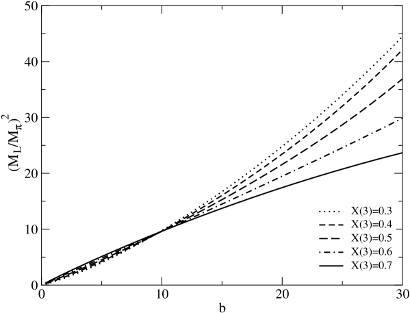
Figure 6: $M_{L}^{2}/M_{\pi}^{2}$ as a function of $b=m_{L}/m$ for $Z(3)=0.6,r=25$. All NNLO remainders are set to zero.

For values of $Z(3)$ between 0.4 and 0.8 and of $r$ between 20 and 30, we find that the allowed region does not qualitatively change: so long as we keep $m_{L}/m$ less than 20, then all values of $X(3)$ are permitted according to our stability criterion. Consider, then, the variation of $F_{L}^{2}$ and of $F_{L}^{2}M_{L}^{2}$ as functions of $m_{L}$, for fixed $Z(3)$ and $r$, as shown in Figs. 7 and 8 in the illustrative case $Z(3)=0.6,r=25$. From Eqs. (142)-(143), the general dependence on $X(3)$ is apparent: the $X(3)$-dependence must vanish for small $b=m_{L}/m$ as well as for $b=m_{L}/m\sim(r+2)/3\sim 10$ (apart from a residual dependence from the logarithms). Therefore, the region of interest is $10\leq b\leq 20$. Fortunately, even in this restricted interval, there is considerable dependence on $X(3)$, especially for $F_{L}^{2}M_{L}^{2}/b$. A good knowledge of the spectrum in this range would allow us to discriminate at least between the most extreme possibilities ($X(3)$ close to $X(2)$, $X(3)$ close to 0). We stress that not all the observables are equivalent for this study: for instance, $M_{L}^{2}$ exhibits a much weaker sensitivity to vacuum fluctuations, as shown in Fig. 6. This cancellation between $L_{6}$ and $L_{4}$ in the case of the masses is quite usual [13] and does not mean that the effect is absent for all observables, as seen from Figs. 7 and 8.

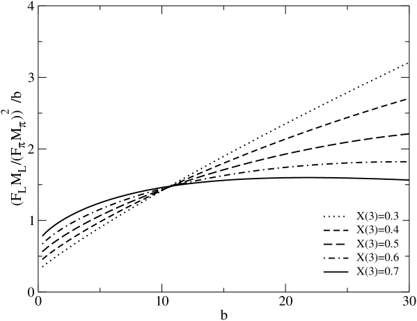
Figure 7: $F_{L}^{2}M_{L}^{2}/(F_{\pi}M_{\pi})^{2}/b$ as a function of $b$. Each line corresponds to a different value of $X(3)$, whereas $r$ is set to 25. All NNLO remainders are set to zero.

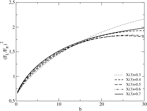
Figure 8: $F_{L}^{2}/F_{\pi}^{2}$ as a function of $b$. Each line corresponds to a different value of $X(3)$, whereas $r$ is set to 25. All NNLO remainders are set to zero.

We have not included the NNLO remainders $d_{L}$ and $e_{L}$ here, but it is a straightforward exercise to take them into account. We can check their size by writing them in the following form:

$$F_{\pi}^{2}M_{\pi}^{2}d_{\pi} = m_{s}^{2}mD_{1}+m_{s}m^{2}D_{2}+m^{3}D_{3}\,,$$

$$F_{\pi}^{2}e_{\pi} = m_{s}^{2}E_{1}+m_{s}mE_{2}+m^{2}E_{3}\,,$$ (144)

where $D_{i}$ and $E_{i}$ do contain $O(p^{6})$ LEC’s and chiral logarithms. If we neglect the dependence of the chiral logarithms on the quark masses when they vary from $m,m_{s}$ to $m_{L}$, the same quantities will appear in the analogous expression for $F_{L}^{2}M_{L}^{2}d_{L},F_{L}^{2}e_{L}$:

$${d_{L}\over d_{\pi}} = \bigg{[}{bF_{\pi}^{2}M_{\pi}^{2}\over F_{L}^{2}M_{L}^{2}}\bigg{]}\ {b^{2}\over r^{2}}\ \bigg{[}{D_{1}+D_{2}+D_{3}\over D_{1}+D_{2}/r+D_{3}/r^{2}}\bigg{]}\,,$$

$${e_{L}\over e_{\pi}} = \bigg{[}{F_{\pi}^{2}\over F_{L}^{2}}\bigg{]}\ {b^{2}\over r^{2}}\ \bigg{[}{E_{1}+E_{2}+E_{3}\over E_{1}+E_{2}/r+E_{3}/r^{2}}\bigg{]}\,.$$ (145)

We can check easily that the first factor is of order one in each case (see for instance Figs. 7 and 8). Therefore, we conclude that the remainders $d_{L},e_{L}$ are expected to be of order $m_{L}^{2}$, i.e., of order $0.1\cdot b^{2}/r^{2}$ (i.e., 10 % or less). Once the remainders are included, an accurate determination of $Z(3)$ is quite difficult because $F_{L}^{2}$ does not exhibit a strong sensitivity to the latter. But $X(3)$ is still accessible because of the strong variation in the curvature of $F_{L}^{2}M_{L}^{2}$ as a function of $b$.

6 Summary and conclusion

The large-$N_{c}$ suppressed low-energy constants $L^{r}_{4}(\mu)$ and $L^{r}_{6}(\mu)$ encode fluctuations of vacuum $\bar{s}s$ pairs. We have analysed the influence of these fluctuations on the convergence of $N_{f}=3$ $\chi$PT.

• For the physical value of $m_{s}$, we assume a global (though possibly slow) convergence of the $SU(3)\times SU(3)$ chiral expansion applied to low-energy connected QCD correlation functions and to observables that are linearly related to the latter: typical examples are $F^{2}_{P}$, $F^{2}_{P}M^{2}_{P}$, $F^{4}_{\pi}A_{\pi\pi\to\pi\pi}$ , $F^{2}_{\pi}F^{2}_{K}A_{\pi K\to\pi K}$, etc. For such quantities, the bare expansion (as defined in Sec. 2) expressed in terms of the order parameters $\Sigma(3)$ and $F_{0}$ and in powers of quark masses $m_{u},m_{d},m_{s}$ is likely characterised by relatively small higher-order corrections starting at NNLO.

• Vacuum fluctuations of $\bar{s}s$ pairs affect in particular the next-to-leading-order (NLO) contributions to $F^{2}_{\pi}M^{2}_{\pi}$ and $F^{2}_{\pi}$ through terms $m_{s}L_{6}$ and $m_{s}L_{4}$, which appear in $\chi$PT with large coefficients. They reflect Zweig-rule violation and large $1/N_{c}$ corrections in the scalar channel. Unless $L_{6}$ and $L_{4}$ are very precisely tuned to their critical values $L^{\rm crit}_{6}(M_{\rho})=-0.26\cdot 10^{-3}$, $L^{\rm crit}_{4}(M_{\rho})=-0.51\cdot 10^{-3}$, the vacuum fluctuation NLO contribution to $F^{2}_{\pi}M^{2}_{\pi}$ and/or to $F^{2}_{\pi}$ becomes of comparable size or even larger than the corresponding leading-order (LO) contributions given by the three-flavour condensate $\Sigma(3)$ and by the pion decay constant $F^{2}_{0}$. In this case, the expansions of $X(3)=2m\Sigma(3)/F^{2}_{\pi}M^{2}_{\pi}$ and $Z(3)=F^{2}_{0}/F^{2}_{\pi}$ in powers of $m_{s}$ break down despite the convergence of $F^{2}_{\pi}M^{2}_{\pi}$ and $F^{2}_{\pi}$. As a result, $X(3)$ and $Z(3)$, which measure $N_{f}=3$ order parameters in physical units, could be suppressed well below one, implying an instability of $N_{f}=3$ $\chi$PT.

• The instability due to vacuum fluctuations upsets the standard perturbative reexpression of the lowest order parameters $\Sigma(3)$ and $F^{2}_{0}$ as well as quark masses in favour of an expansion in terms of physical Goldstone boson masses, $F_{\pi}$ and $F_{K}$. Instead, using the four mass and decay constant Ward identities, we nonperturbatively eliminate the LEC’s $L_{4},L_{5},L_{6},(L_{7}),L_{8}$ in terms of the order parameters $X(3)$ and $Z(3)$ , the quark mass ratio $r=m_{s}/m$ and four NNLO remainders $d_{\pi},d_{K},e_{\pi},e_{K}$ which collect all higher-order contributions starting at $O(p^{6})$. This procedure amounts to an exact resummation of the standard perturbative reexpression of $X(3)$, $Z(3)$ and $r$ and it applies even if the vacuum fluctuations suppress $X(3)$ and/or $Z(3)$.

• In this way, values of the basic order parameters $X(3)$, $Z(3)$ and the quark mass ratio $r$ can be constrained by experimental data as long as NNLO remainders are under control. In order to gradually incorporate theoretical conjectures about the order parameters $X(3)$ and $Z(3)$ (e.g., their positivity, paramagnetic inequalities), and on higher chiral orders (i.e., NNLO remainders), we propose to use Bayesian statistical inference. In this approach, previous knowledge of parameters is encoded into the prior probability distribution function. At this step, some degree of arbitrariness is introduced, but the dependence on the choice of the prior is guaranteed to be weak if data are significant enough.

• We have applied this procedure to the three-flavour analysis of elastic $\pi\pi$ scattering, in order to test the ability of the recent high-precision low-energy data obtained by the E865 Collaboration [14] to constrain three-flavour chiral dynamics. We have shown that, for the present state of experimental precision, the data cannot determine the two fundamental $N_{f}=3$ chiral order parameters $X(3)$ and $Z(3)$. However, the low-energy $\pi\pi$ data is sufficient for us to put a quantitative lower bound on the quark mass ratio $r=m_{s}/m\geq 14$ at the 95% confidence level, and to determine the corresponding probability distribution function.

• The Bayesian machinery is suitable for incrementally including further experimental information on low-energy observables, and seems especially well-adapted in this context, in view of an extension of our analysis to valence $s$-quark effects. In particular, $\pi K$ scattering appears to be rather promising, due to recent progress obtained through the solution of the corresponding Roy-Steiner equations [33]. We plan to address this issue in future publications [26].

• The possible instability of $N_{f}=3$ chiral expansions, and the prescription examined in this paper to treat it, are also relevant in other respects. One example is the evaluation of $K\rightarrow\pi\pi$ weak matrix elements from sum rules based on OPE: in particular, the extrapolation of the OPE condensate from the chiral limit to physical values of quark masses would not be possible on the basis of the usual treatment of $N_{f}=3$ $\chi$PT formulas. A similar remark applies to the study of the quark mass dependence of Goldstone boson masses on the lattice and to determinations of the LEC’s by this means. We have shown how such a program could be pursued even in the presence of large fluctuations, provided simulations with three dynamical flavours would be available with quark masses as small as the physical strange quark mass. It remains to be seen whether such simulations, with proper control of the continuum and thermodynamic limits, will be feasible in the near future.

• In order to detect possibly large $\bar{s}s$ fluctuations, another strategy is conceivable: one might calculate and analyse as many quantities as possible within the standard $SU(3)\times SU(3)$ $\chi$PT, up to and including two loops, using the standard perturbative reexpression of low-energy parameters [17, 20]. The instability of such $\chi$PT expansions could appear as an internal inconsistency of the result of corresponding fits with the assumptions underlying the perturbative treatment of standard $\chi$PT.

Appendix A Mass and decay constant identities

We recall for convenience the chiral expansion of Goldstone boson masses as discussed in Refs. [11, 13]:

$$F_{\pi}^{2}M_{\pi}^{2} = 2m\Sigma(3)+2m(m_{s}+2m)Z^{s}+4m^{2}A+4m^{2}B_{0}^{2}L+F_{\pi}^{2}M_{\pi}^{2}d_{\pi},\qquad$$ (146)

$$F_{K}^{2}M_{K}^{2} = (m_{s}+m)\Sigma(3)+(m_{s}+m)(m_{s}+2m)Z^{s}+(m_{s}+m)^{2}A$$

$$\quad+m(m_{s}+m)B_{0}^{2}L+F_{K}^{2}M_{K}^{2}d_{K},$$

The case of the $\eta$-meson is discussed in Sec. 3.4 and below. The connection with the standard LEC’s of the $N_{f}\geq 3$ effective Lagrangian is:

$$Z^{s} = 32B_{0}^{2}\left\{L_{6}(\mu)-\frac{1}{512\pi^{2}}\left[\log\frac{M_{K}^{2}}{\mu^{2}}+\frac{2}{9}\log\frac{M_{\eta}^{2}}{\mu^{2}}\right]\right\},$$ (148)

$$A = 16B_{0}^{2}\left\{L_{8}(\mu)-\frac{1}{512\pi^{2}}\left[\log\frac{M_{K}^{2}}{\mu^{2}}+\frac{2}{3}\log\frac{M_{\eta}^{2}}{\mu^{2}}\right]\right\}.$$ (149)

The remainders $F_{P}^{2}M_{P}^{2}d_{P}$ collect all higher-order terms, starting at the next-to-next-to-leading order $O(m_{q}^{3})$, in agreement with the definition in Ref. [13], but different from that in Ref. [8]. The combination of chiral logarithms $L$ is [13]:

$$L=\frac{1}{32\pi^{2}}\left[3\log\frac{M_{K}^{2}}{M_{\pi}^{2}}+\log\frac{M_{\eta}^{2}}{M_{K}^{2}}\right].$$ (150)

Similar expressions are derived for the decay constants:

$$F_{\pi}^{2} = F^{2}(3)+2(m_{s}+2m)\tilde{\xi}+2m\xi$$

$$\quad+\frac{1}{16\pi^{2}}2mB_{0}\left\{\log\frac{M_{\eta}^{2}}{M_{K}^{2}}+2\log\frac{M_{K}^{2}}{M_{\pi}^{2}}\right\}+F_{\pi}^{2}e_{\pi}\qquad$$

$$F_{K}^{2} = F^{2}(3)+2(m_{s}+2m)\tilde{\xi}+(m_{s}+m)\xi+mB_{0}L+F_{K}^{2}e_{K}$$ (152)

The scale-invariant constants $\xi$ and $\tilde{\xi}$ are related to the LEC’s $L_{4}$ and $L_{5}$ as follows:

$$\tilde{\xi} = 8B_{0}\left\{L_{4}(\mu)-\frac{1}{256\pi^{2}}\log\frac{M_{K}^{2}}{\mu^{2}}\right\}\,$$ (153)

$$\xi = 8B_{0n}\left\{L_{5}(\mu)-\frac{1}{256\pi^{2}}\left[\log\frac{M_{K}^{2}}{\mu^{2}}+2\log\frac{M_{\eta}^{2}}{\mu^{2}}\right]\right\}.$$ (154)

The remainders $F_{P}^{2}e_{P}$ collect the NNLO terms $O(m_{q}^{2})$. Eqs. (32), (40)-(41) in Sec. 3.2 can be obtained by combining the previous identities to eliminate the $O(p^{4})$ LEC’s $A,Z_{S},\xi,\tilde{\xi}$.

The identities for the $\eta$ can be recast in a form reminiscent of the Gell-Mann–Okubo formula:

$$3F_{\eta}^{2}M_{\eta}^{2}-4F_{K}^{2}M_{K}^{2}+F_{\pi}^{2}M_{\pi}^{2}$$ (155)

$$\quad=4(r-1)m^{2}\left\{(r-1)(2Z^{p}+A)-B^{2}_{0}L\right\}+3F_{\eta}^{2}M_{\eta}^{2}d_{\eta}-4F_{K}^{2}M_{K}^{2}d_{K}+F_{\pi}^{2}M_{\pi}^{2}d_{\pi}\,,$$

$$3F_{\eta}^{2}-4F_{K}^{2}+F_{\pi}^{2}$$ (156)

$$\quad=\frac{2mB_{0}}{16\pi^{2}}\left[(1+2r)\log\frac{M_{\eta}^{2}}{M_{K}^{2}}-\log\frac{M_{K}^{2}}{M_{\pi}^{2}}\right]+3F_{\eta}^{2}e_{\eta}-4F_{K}^{2}e_{K}+F_{\pi}^{2}e_{\pi}\,.$$

The $\eta$-mass identity involves the new LEC $Z^{p}=16B_{0}^{2}L_{7}$. We have also introduced the NNLO remainders $d_{\eta}$ and $e_{\eta}$ of order $O(m_{q}^{2})$.

Appendix B $\mathbf{\chi}$PT and Bayesian statistical analysis

One of the main achievements of $SU(3)\times SU(3)$ chiral perturbation theory consists in providing a consistent framework that includes all the constraints of chiral symmetry when one analyses processes involving the Goldstone bosons $\pi,K,\eta$. This allows one to express observables as expansions in powers of momenta and quark masses up to a given order. Each order involves new low-energy constants whose values cannot be determined from chiral constraints, but nevertheless provide very much needed insight into the mechanism of chiral symmetry breaking.

We would like therefore to pin down (or at least constrain) LEC’s arising at first order in $SU(3)\times SU(3)$ chiral expansions – for instance, the quark condensate and the pseudoscalar decay constant in the limit $m_{u},m_{d},m_{s}\to 0$ – by using available experimental information.

We must therefore combine several sources of information:

• Experimental measurements of observables $\alpha_{i}$: $P^{\exp}_{j}(\alpha_{i})$

  Their values have (possibly correlated) uncertainties which are described by probability distributions. In the theoretical basis that underlies the determination of these observables no use of $\chi$PT should have been made. For instance, solutions of Roy equations were required in addition to experimental phase shifts to extract $\pi\pi$ scattering parameters. As explained in Sec. 2.3, a reasonable choice of observables can be derived from QCD correlation functions of currents and densities, away from kinematic singularities; e.g., one may choose $\pi\pi$ subthreshold parameters.

• Relations between the observables and theoretical parameters $T_{n}$: $\alpha_{i}={\mathcal{A}}_{i}(T_{n})$

  We have explained how mass and decay constant identities can be used to eliminate some $O(p^{4})$ LEC’s in chiral expansions of observables. We have chosen the theoretical parameters to be $X(3)$, $Z(3)$, $r$, and remainders that comprise NNLO and higher order corrections.

• Theoretical constraints/assumptions about the values of $T_{n}$: ${\mathcal{C}}_{k}(T_{n})$

  Chiral order parameters are constrained: for instance, vacuum stability requires $X(3)\geq 0$, whereas $Z(3)$ is positive by definition. We have also theoretical prejudices about NNLO remainders if we require an overall convergence of chiral expansions: the relative contribution of NNLO remainders must remain small.

It is quite easy from these elements to construct the likelihood function

$$\mathcal{L}(T_{n})=P({\rm data}|T_{n},H)=\prod_{j}P^{\exp}_{j}[{\mathcal{A}}_{i}(T_{n})]\,,$$ (157)

which is the probability of obtaining the observed data once a particular set of theoretical parameters is given (within the theoretical framework $H$). However, what we want is not $\mathcal{L}$, but rather the reverse quantity $P(T_{n}|{\rm data},H)$, i.e., the probability of having a particular set of theoretical parameters, taking into account the data.

This problem of “statistical inference” has a long history. A possible solution is provided by Bayesian analysis [22], which relies on Bayes’ theorem:

$$P(T_{n}|{\rm data},H)=\frac{\mathcal{L}(T_{n})\cdot\pi(T_{n}|H)}{\int\ [dT]\ \mathcal{L}(T_{n})\cdot\pi(T_{n}|H)}\,,$$ (158)

where $\pi$ is the “prior” distribution, i.e., the probability associated with the theoretical parameters before the experimental results have been taken in consideration:

$$\pi(T_{n})=P(T_{n}|H)=\prod_{k}{\mathcal{C}}_{k}(T_{n})\,.$$ (159)

The denominator on the right-hand side of Eq. (158) is just a normalisation factor. The marginal probability associated with a given theoretical parameter is obtained by integrating the joint probability $P(T_{n}|{\rm data},H)$ over all other theoretical parameters.

Let us mention that there is some arbitrariness in each of these ingredients. We could have chosen other observables, such as combinations of scattering lengths in which one-loop chiral logarithms cancel [32]. We could have added all $O(p^{4})$ LEC’s to the set of theoretical parameters, and kept “bare” chiral expansions as relations among the observables. Finally, we could have computed $O(p^{6})$ contributions to NNLO remainders and used resonance saturation to estimate the size of the remainders, following the procedure in Ref. [17].

In the present paper we have advocated a particular choice of observables as constituting a sensible starting point for a Bayesian analysis of data from $\pi\pi$ and $\pi K$ scattering. Other choices of prior p.d.f’s for the theoretical parameters (especially for the NNLO remainders) can be considered, as long as they are well motivated. However, the posterior probabilities should not be strongly sensitive to the choice of priors when a sufficient amount of experimental data is included in the analysis.

Appendix C Integration procedure for the analysis of $\pi\pi$ scattering

In Sec. 4, we apply Bayesian methods to perform a three-flavour analysis of $\pi\pi$ scattering, constructing a joint probability $P(r,Y,Z,\vec{\delta}|{\rm data})$. This gives the probability of having a particular choice of quark mass ratio $r$, order parameters $Y(3)$ and $Z(3)$ and NNLO remainders $\delta_{i=1\ldots 7}$, once $\pi\pi$ scattering data is taken into account. By integrating over NNLO remainders, we obtain the joint probability

$$P(r,Y,Z|{\rm data}) = \int\prod_{i=1}^{7}d\delta_{i}\ P(r,Y,Z,\vec{\delta}|{\rm data})$$ (161)

$$\propto \pi(Y,Z)\ \theta(r-r_{1})\ \theta(r_{2}-r)\ \theta[Z(3)]\ \theta[Y(3)]\$$

$$\quad\times\int^{\delta_{1}^{\rm max}}\!\!\!d\delta_{1}\int^{\delta_{2}^{\rm max}}\!\!\!d\delta_{2}\int_{\delta_{6}^{\rm min}}d\delta_{6}\int_{\delta_{7}^{\rm min}}d\delta_{7}\int d\delta_{3}\ d\delta_{4}\ d\delta_{5}$$

$$\quad\times\prod_{i=1}^{7}G(\delta_{i},\sigma_{i})\exp\left(-\frac{1}{2}{\mathcal{V}}^{T}C{\mathcal{V}}\right)\theta[Y^{\rm max}-Y(3)]\,,$$

where $\propto$ means “equals, up to a (numerical) normalization coefficient”, $C$ is the error matrix for the experimental data, Eq. (4.2), $G(\delta_{i},\sigma_{i})$ is the Gaussian function of $\delta_{i}$ with width $\sigma_{i}$, and ${\mathcal{V}}$ is defined in terms of the chiral series for $\alpha_{\pi\pi}$ and $\beta_{\pi\pi}$, Eqs. (96)-(97):

$${\mathcal{V}}(r,Y,Z,\vec{\delta})=\left(\begin{array}[]{c}{\mathcal{A}}(r,Y,Z,\vec{\delta})-\alpha_{\exp}\\ {\mathcal{B}}(r,Y,Z,\vec{\delta})-\beta_{\exp}\end{array}\right)\,.$$ (162)

Before any numerical evaluation, we can analytically compute some of the integrals. $\delta_{4}$ and $\delta_{5}$ have the same width $\sigma_{4}=\sigma_{5}$ and appear only in the experimental distribution obtained from $\pi\pi$ scattering. We can therefore diagonalize the latter

$$R^{T}R=RR^{T}=I\,,\qquad RCR^{T}=\left[\begin{array}[]{cc}C_{1}&0\\ 0&C_{2}\end{array}\right]\,,$$ (163)

to perform the integration  over $\delta_{4}$ and $\delta_{5}$:

$$\int\delta_{4}\,\delta_{5}\,G(\delta_{4},\sigma_{4})G(\delta_{5},\sigma_{4})\exp\left(-\frac{1}{2}{\mathcal{V}}^{T}C{\mathcal{V}}\right)\propto\exp\left[-\frac{1}{2}(D_{1}{\mathcal{W}_{1}}+D_{2}{\mathcal{W}_{2}})\right]\,,$$ (164)

$$D_{i}=\frac{C_{i}}{1+C_{i}\sigma_{4}^{2}}\,,\qquad{\mathcal{W}}=R\cdot{\mathcal{V}}(r,Y,Z,\delta_{1,2,3};\delta_{4}=\delta_{5}=0)\,.$$ (165)

The integrals over $\delta_{6}$ and $\delta_{7}$ are simply Gaussians integrated over semi-infinite ranges, and are thus given in terms of the error function ${\rm Erf}$. We obtain finally:

$$P(r,Y,Z|{\rm data})\propto\pi(Y,Z)\ \theta(r-r_{1})\ \theta(r_{2}-r)\ \theta[Z(3)]\ \theta[Y(3)]$$

$$\quad\times\int^{\delta_{1}^{\rm max}}\!\!\!d\delta_{1}\int^{\delta_{2}^{\rm max}}\!\!\!d\delta_{2}\int d\delta_{3}\prod_{i=1}^{3}G(\delta_{i},\sigma_{i})\exp\left[-\frac{1}{2}(D_{1}{\mathcal{W}_{1}}+D_{2}{\mathcal{W}_{2}})\right]$$

$$\quad\times\left[1-{\rm Erf}\left(\frac{\delta_{6}^{\rm min}}{\sqrt{2}\sigma_{6}}\right)\right]\left[1-{\rm Erf}\left(\frac{\delta_{7}^{\rm min}}{\sqrt{2}\sigma_{7}}\right)\right]\theta[Y^{\rm max}-Y(3)]\,.$$ (166)

In order to obtain the marginal probability for either $r$, $X(3)$, $Y(3)$ or $Z(3)$, we must perform a numerical integration over 3 remainders to obtain the joint probability $P(r,Y,Z|{\rm data})$, and then integrate the result over two of the remaining three parameters. We restrict the integration over the remainders $\delta_{1,2,3}$ to the range $[-5\sigma_{i},5\sigma_{i}]$ (the upper bound can be smaller for $i=1,2$ due to the positivity constraints Eqs. (111)-(112)). The range of integration for the two parameters that remain to be integrated is given by the theoretical constraints discussed in Sec. 4.

In order to appreciate the impact of data in the Bayesian framework, it is quite interesting to consider the marginal probabilities obtained when no experimental information is included. In our particular case, this amounts to replacing the experimental distribution $P_{\exp}(\alpha,\beta)$ by 1, or equivalently to setting the matrix $C$ to 0. We obtain then the following p.d.f:

$$P_{0}(r,Y,Z|{\rm data})\propto\pi(Y,Z)\ \theta(r-r_{1})\ \theta(r_{2}-r)\ \theta[Z(3)]\ \theta[Y(3)]$$

$$\quad\times\int^{\delta_{1}^{\rm max}}\!\!\!d\delta_{1}\int^{\delta_{2}^{\rm max}}\!\!\!d\delta_{2}\int d\delta_{3}\prod_{i=1}^{3}G(\delta_{i},\sigma_{i})\theta[Y^{\rm max}-Y(3)]$$

$$\quad\times\left[1-{\rm Erf}\left(\frac{\delta_{6}^{\rm min}}{\sqrt{2}\sigma_{6}}\right)\right]\left[1-{\rm Erf}\left(\frac{\delta_{7}^{\rm min}}{\sqrt{2}\sigma_{7}}\right)\right]\,.$$ (167)

$P_{0}$ is just the normalized prior p.d.f, and corresponds to the “phase space” allowed by the theoretical constraints and assumptions on the various parameters. The resulting marginal probabilities can be found in Sec. 4, where they are compared with the ones that include experimental knowledge about $\pi\pi$ scattering.

References

- [1] J. Gasser and H. Leutwyler, Ann. Phys. (NY) 158 (1984) 142.
- [2] S. Chen, M. Davier, E. Gámiz, A. Hocker, A. Pich and J. Prades, Eur. Phys. J. C 22 (2001) 31 [hep-ph/0105253]. E. Gámiz, M. Jamin, A. Pich, J. Prades and F. Schwab, J. High Energy Phys. 0301 (2003) 060 [hep-ph/0212230].
- [3] J. Gasser and H. Leutwyler, Nucl. Phys. B 250 (1985) 465.
- [4] M. Boglione and M. R. Pennington, Phys. Rev. D 65 (2002) 114010 [hep-ph/0203149]. S. Spanier and N. Törnqvist in K. Hagiwara et al. [Particle Data Group Collaboration], Phys. Rev. D 66 (2002) 010001.
- [5] B. Moussallam, Eur. Phys. J. C 14 (2000) 111 [hep-ph/9909292].
- [6] B. Moussallam, J. High Energy Phys. 0008 (2000) 005 [hep-ph/0005245].
- [7] S. Descotes-Genon and J. Stern, Phys. Lett. B 488 (2000) 274 [hep-ph/0007082].
- [8] S. Descotes-Genon, J. High Energy Phys. 0103 (2001) 002 [hep-ph/0012221].
- [9] T. Appelquist and S. B. Selipsky, Phys. Lett. B 400 (1997) 364 [hep-ph/9702404]. M. Velkovsky and E. V. Shuryak, Phys. Lett. B 437 (1998) 398 [hep-ph/9703345].
- [10] T. Banks and A. Casher, Nucl. Phys. B 169 (1980) 103. H. Leutwyler and A. Smilga, Phys. Rev. D 46 (1992) 5607. J. Stern, hep-ph/9801282. S. Descotes-Genon and J. Stern, Phys. Rev. D 62 (2000) 054011 [hep-ph/9912234].
- [11] S. Descotes-Genon, L. Girlanda and J. Stern, J. High Energy Phys. 0001 (2000) 041 [hep-ph/9910537].
- [12] L. Girlanda, J. Stern and P. Talavera, Phys. Rev. Lett. 86 (2001) 5858 [hep-ph/0103221].
- [13] S. Descotes-Genon, L. Girlanda and J. Stern, Eur. Phys. J. C 27 (2003) 115 [hep-ph/0207337].
- [14] S. Pislak et al. [BNL-E865 Collaboration], Phys. Rev. Lett. 87 (2001) 221801 [hep-ex/0106071]; Phys. Rev. D 67 (2003) 072004 [hep-ex/0301040].
- [15] S. Descotes-Genon, N. H. Fuchs, L. Girlanda and J. Stern, Eur. Phys. J. C 24 (2002) 469 [hep-ph/0112088].
- [16] J. Bijnens, G. Ecker and J. Gasser, published in 2nd DAPHNE Physics Handbook (125-140), L. Maiani, G. Pancheri and N. Paver Eds. [hep-ph/9411232].
- [17] G. Amoros, J. Bijnens and P. Talavera, Nucl. Phys. B 568 (2000) 319 [hep-ph/9907264]; Nucl. Phys. B 585 (2000) 293 [Erratum-ibid. B 598 (2000) 665] [hep-ph/0003258].
- [18] J. Bijnens, G. Colangelo and P. Talavera, J. High Energy Phys. 9805 (1998) 014 [hep-ph/9805389]. J. Bijnens, P. Dhonte and F. Persson, Nucl. Phys. B 648 (2003) 317 [hep-ph/0205341].
- [19] B. Ananthanarayan and P. Büttiker, Eur. Phys. J. C 19 (2001) 517 [hep-ph/0012023]. B. Ananthanarayan, P. Büttiker and B. Moussallam, Eur. Phys. J. C 22 (2001) 133 [hep-ph/0106230].
- [20] J. Bijnens and P. Dhonte, hep-ph/0307044.
- [21] N. H. Fuchs, H. Sazdjian and J. Stern, Phys. Lett. B 269 (1991) 183; J. Stern, H. Sazdjian and N. H. Fuchs, Phys. Rev. D 47 (1993) 3814 [hep-ph/9301244]. M. Knecht and J. Stern, published in 2nd DAPHNE Physics Handbook (169-190), L. Maiani, G. Pancheri and N. Paver Eds. [hep-ph/9411253].
-
[22]
D. Silvia, Data Analysis - A Bayesian Tutorial,
Clarendon Press (1996).
G. D’Agostini,
Cern Yellow Report, CERN-99-03,
[http://preprints.cern.ch/cgi-bin/setlink?base=cernrep&categ=Yellow_Report&id=99-03]
Additional references can be found on
http://astrosun.tn.cornell.edu/staff/loredo/bayes/ For recent discussions of the Bayesian and frequentist approaches to the determination of CKM-matrix elements, see M. Ciuchini et al., J. High Energy Phys. 0107 (2001) 013 [hep-ph/0012308]. A. Höcker, H. Lacker, S. Laplace and F. Le Diberder, Eur. Phys. J. C 21 (2001) 225 [hep-ph/0104062]. - [23] J. Bijnens, G. Colangelo and G. Ecker, J. High Energy Phys. 9902 (1999) 020 [hep-ph/9902437]. J. Bijnens, G. Colangelo and G. Ecker, Ann. Phys. (NY) 280 (2000) 100 [hep-ph/9907333]. J. Bijnens, L. Girlanda and P. Talavera, Eur. Phys. J. C 23 (2002) 539 [hep-ph/0110400].
- [24] M. Knecht, B. Moussallam, J. Stern and N. H. Fuchs, Nucl. Phys. B 457 (1995) 513 [hep-ph/9507319].
- [25] V. Bernard, N. Kaiser and U. G. Meissner, Nucl. Phys. B 357 (1991) 129; Phys. Rev. D 43 (1991) 2757.
- [26] S. Descotes-Genon, N. H. Fuchs, L. Girlanda and J. Stern, in preparation.
- [27] J. Bijnens, Phys. Rept. 265 (1996) 369 [hep-ph/9502335]. G. Ecker, J. Gasser, A. Pich and E. de Rafael, Nucl. Phys. B 321 (1989) 311.
- [28] H. Leutwyler, Nucl. Phys. B 337 (1990) 108.
- [29] L. Girlanda, Phys. Lett. B 513 (2001) 103 [hep-ph/0104270].
- [30] B. Ananthanarayan, G. Colangelo, J. Gasser and H. Leutwyler, Phys. Rev. 353 (2001) 207 [hep-ph/0005297].
- [31] D. B. Kaplan and A. V. Manohar, Phys. Rev. Lett. 56 (1986) 2004.
- [32] G. Colangelo, J. Gasser and H. Leutwyler, Phys. Lett. B 488 (2000) 261 [hep-ph/0007112]. G. Colangelo, J. Gasser and H. Leutwyler, Nucl. Phys. B 603 (2001) 125 [hep-ph/0103088]. G. Colangelo, J. Gasser and H. Leutwyler, Phys. Rev. Lett. 86 (2001) 5008 [hep-ph/0103063].
- [33] P. Büttiker, S. Descotes-Genon and B. Moussallam, hep-ph/0310283.
- [34] J. Gasser and H. Leutwyler, Nucl. Phys. B 250 (1985) 539. A. V. Anisovich and H. Leutwyler, Phys. Lett. B 375 (1996) 335 [hep-ph/9601237]. M. Walker, “”, Master Thesis, University of Bern (1998). Can be obtained from http://www-itp.unibe.ch/research.shtml#diploma. J. Bijnens and J. Gasser, Phys. Scripta T99 (2002) 34 [hep-ph/0202242].
- [35] J. Bijnens, J. Prades and E. de Rafael, Phys. Lett. B 348 (1995) 226 [hep-ph/9411285]. S. Narison, hep-ph/0202200.
- [36] J. Kambor and K. Maltman, Phys. Rev. D 62 (2000) 093023 [hep-ph/0005156]; Phys. Lett. B 517 (2001) 332 [hep-ph/0107060].
- [37] M. Jamin, J. A. Oller and A. Pich, Eur. Phys. J. C 24 (2002) 237 [hep-ph/0110194].
- [38] M. Jamin, Phys. Lett. B 538 (2002) 71 [hep-ph/0201174].
- [39] V. Cirigliano, E. Golowich and K. Maltman, Phys. Rev. D 68 (2003) 054013 [hep-ph/0305118]. J. F. Donoghue and E. Golowich, Phys. Lett. B 478 (2000) 172 [hep-ph/9911309]. J. Bijnens, E. Gamiz and J. Prades, J. High Energy Phys. 0110 (2001) 009 [hep-ph/0108240].
- [40] P. H. Ginsparg and K. G. Wilson, Phys. Rev. D 25 (1982) 2649. D. B. Kaplan, Phys. Lett. B 288 (1992) 342 [hep-lat/9206013]. H. Neuberger, Phys. Lett. B 417 (1998) 141 [hep-lat/9707022], Phys. Lett. B 427 (1998) 353 [hep-lat/9801031]. M. Lüscher, Phys. Lett. B 428 (1998) 342 [hep-lat/9802011].
- [41] R. Frezzotti and G. C. Rossi, hep-lat/0306014.
- [42] L. Susskind, Phys. Rev. D 16 (1977) 3031. H. S. Sharatchandra, H. J. Thun and P. Weisz, Nucl. Phys. B 192 (1981) 205. H. Kluberg-Stern, A. Morel, O. Napoly and B. Petersson, Nucl. Phys. B 220 (1983) 447.
- [43] D. R. Nelson, G. T. Fleming and G. W. Kilcup, Phys. Rev. Lett. 90 (2003) 021601 [hep-lat/0112029].