Abstract

Co-operation of the Feynman DIagram ANAlyzer (DIANA) with the underlying operational system (UNIX) is presented. We discuss operators to run external commands and a recent development of parallel processing facilities and an extension in the spirit of a component model.

1 Introduction

We have developed the program DIANA (DIagram ANAlyser), which allows to calculate Feynman diagrams as ‘input’ for further formulae manipulating languages (mainly FORM [1]) [2], [3] (see also http://www.physik.uni-bielefeld.de/~tentukov/diana.html). Meanwhile there exists a series of applications [4], which would not have been possible without DIANA.

The problem is that in order to cope with the high precision experiments of present-day high energy accelerators, the corresponding calculations within the ‘Standard Model’ (SM) of elementary particle physics must be of similar precision. This means, e.g., for 1-loop approximations even for $2\to 2$ processes the calculation of the order of several hundred diagrams. This number increases rapidly with the number of external legs and/or the number of loops such that one is easily forced to calculate a number of diagrams of the order of thousands. For this one needs an automation to generate the diagrams and this is what DIANA does.

Having produced the FORM ‘input’ for each of the diagrams, in a next step the execution of the FORM program has to run for each diagram separately and the analytic result of all the separate calculations has to be summed up. In many cases like e.g. 1-loop $2\to 2$ calculations the execution time of the FORM jobs is still relatively short and one can just run the corresponding jobs one after the other (e.g. in terms of ‘folders’). In more complicated cases, however, not only the number of diagrams increases but also the analytic calculation of the single diagrams gets more and more time consuming. Here it pays to distribute the essentially independent calculations of the separate diagrams over different computers. In the project described here we have extended DIANA to be able to perform this task and we give detailed hints for potential users of how to apply it.

The program DIANA, written in C, contains two ingredients:

1. Analyzer of diagrams.

2. Interpreter of a special text manipulating (TM) language.

The analyzer reads QGRAF [5] output and passes the necessary information to the interpreter. For each diagram the interpreter performs the TM program, producing input for further evaluation (e.g. by means of FORM) of the diagram. The TM language is a TeX-like language. The main goal of the language is the creation of text files.

Similar to the TeX language, each command has to begin with an escape (“$\backslash$”) character. All lines without escape - characters are simply typed to the output file. Some of the TM commands are built-in TM operators while some are user-defined functions (returning a value) written in the TM language itself.

The main goal of parallel processing is to reduce wall-clock time which is the users waiting time. Parallelism doesn’t come for free; always it has some overhead with respect to serial execution, but it can significantly reduce the wall-clock time.

Not every problem can be divided into parallel tasks. An example of a parallelizable problem is the multiplication of two matrices. An example of a non-parallelizable problem is the calculation of the Fibonacci series (1,1,2,3,5,…) by means of the formula $F(k+2)=F(k+1)+F(k)$.

Computations in perturbative Quantum Field Theory involve the calculation of Feynman diagrams. DIANA is used to produce the input for their further analytic evaluation. In fact DIANA needs a “model file” produced by the user and then generates the “input” in terms of formally defined vertices and propagators and of coupling parameters [3]. This generation of Feynman diagrams itself is not a good parallelizable problem. Moreover, the time DIANA spends to produce such input is negligible with respect to the time used for the diagram evaluation. Thus the present approach consists in generating input for each diagram sequentially, with the possibility to parallelize the further evaluation.

After the diagrams are generated, DIANA may be used as a “control center” for further evaluations (in parallel) by invoking the corresponding programs and providing them the generated input. To avoid a cluster/processor overloading, each time only one job per node/processor is actually running while all the rest is queued. Such an approach is known as a Batch Queueing System (BQS). There exist a lot of such systems, both free and commercial [6]. Usually, these systems are aimed to deal with a big number of different isolated tasks, while in our case we have a huge number of nearly even tasks.

There are two kinds of optimization of BQS available. The first is for the case when the average number of jobs is much larger than the number of nodes. In this case BQS usually provides various complicated methods for scheduling, message pasting, job run-time quotas and resource management in order to distribute computational resources among various tasks of all kinds. In our case all these mechanisms are not needed. Secondly, if the average number of jobs is comparable with the number of nodes, which is typical for parallel computation, a BQS should provide load balancing, process migration mechanisms and some others.

Compared to that, DIANA has to implement parallelism in terms of job queueing, and the typical situation consists of a long queue of nearly even tasks with the same priority. Evidently, we need not any load balancing. Indeed, the best procedure is to send a new task to a node immediately when the node becomes free. Thus, the real problem in our case is the problem of synchronization. Traditionally, this problem is ignored in BQS since all jobs are assumed to be completely independent. The synchronization problem arises in true parallel systems. Since we use queueing in order to implement a parallelism, the problem is of immediate interest in our case.

The TM language contains several groups of operators permitting DIANA to make a fine co-operation with the underlying operational system (UNIX). The operators \system() and \asksystem() execute an external command synchronously (see sect. 2), i.e. they wait for the command to be completed. The operator \pipe() (sect. 3) starts the external command opening an input-output channel for it, and can be used in order to extend DIANA in the spirit of a component model (sect. 3.4). The term “component model” (see, e.g., [7]) means that a software system is built from “components”. Components are high level aggregations of smaller software pieces, and provide a “black box” building block approach to software construction.

Let us now suppose that we use a cluster with disk space shared by means of NFS, and all results must be collected into one resulting file log.all, while every job produces a file log.# where # is the order number of the job. Since jobs are running and completing independently of each other, we can only collect all log.# into log.all after all the jobs are finished. This leads to producing a lot of files log.# at an intermediate step, which can overload a file system.

The simple solution is to allow some of the newly started jobs to be synchronized with all previously started jobs. Indeed, in this case after each job we can start another “slave” job, which appends the log.# file containing the result of the “master” job to the file log.all. To obtain a correct order of the file log.all, this copying job must be performed only after all earlier jobs are finished.

Another problem with cluster computations is that the optimal placement of the resulting file log.# is usually a /tmp directory which is local with regard to the current node, on which the job “number #” is performed. But to do this, the “slave” copying job has to “stick” to the “master” job, i.e. it must be performed on the same node as the “master” job.

Both above mentioned problems are solved by means of so-called job attributes, see sect. 4.2.

Yet another problem is the transaction problem, which in our case means whether a job group should be restarted on failure, and what the failure/success conditions are. Sometimes it is necessary to perform some complicated job with many unreliable intermediate steps (e.g., breakdown of some connection) and at the end return the exit code depending on the status of the whole transaction. In such cases it is useful to have a possibility to restart the job many times. But for conventional jobs consisting of one external program the number of restarts must not be too large in order to permit the user to kill jobs which failed.

Conditions on which a job is assumed to have failed may be rather complicated, too. For example, the above mentioned copying “slave” job is just a quick system command “cp”. The probability of its failure is very low, less then the probability of some network connection failure during the commands initiation. If started, such a job, most probably, will be completed successfully independently of the DIANA client/server status. That is why it is reasonable to assume that the job is successful if it is started by the server. On the other hand, the “master” job is expected to return some exit code, but not to be killed by some signal. For the solution of these problems see sect. 4.2 as well.

The operator \_exec() and companions can be used to define several macros and TM functions in order to create a BQS which meets our requirements; for a simplified example see sect. 4.4. There is the possibility to build a really powerful BQS based on the \_exec() family combined with external components communicating with DIANA through the operator \pipe(). A simplified version of this is demonstrated.

2 Running external commands

The operator \system(command) executes the external command and returns the exit code. Usually, 0 means that the invoked program was executed successfully. Example: \system(ls) types to the screen the content of the current directory and returns 0.

The operator \asksystem(command,text) executes the external command, using the second argument as its “standard input”. It reads the first line of the external command output and stores it. Then the external command is terminated, and the stored line is returned. For example, \asksystem(cat,Hello!) returns the text “Hello!”, but \asksystem(cat,One!\eol()Two!) returns the text “One!” (\eol() is the DIANA command ending the line).

Another example:

\offleadingspaces
  * Host: \asksystem(hostname,); \asksystem(date,)

in the TM program has led to the following line in the produced output:

* Host: phya24; Fri May  30 22:51:38 CET 2003

3 Dialog with an external program

3.1 Starting a pipe

The operator \asksystem() is used to “ask” a single question from the command, as described above. In order to organize a dialog with an external program, the operator \pipe(command) can be used. It starts the command, swallowing its standard input and output. It returns an integer number, a PID of a newly started process, or an empty string, if it fails. Further, the returned PID can be used in order to send some text to the program, or to read program output.

After the operator \pipe() returns the control to the TM program, the program initiated by command continues to run. Its standard input and output references are stored by DIANA. Both input and output are not connected with any terminal device. The running external program is visible from the TM program as a duplex “pipe” identified by the PID of the external program.

The operator \closepipe(rpipe) (here rpipe is the PID of the external program returned by \pipe()) terminates the external program. It closes the programs’ IO channels, sends to the program a KILL signal and waits for the command to be finished.

3.2 Reading and writting with the pipe

There are two operators to write to the pipe. One is \topipe(rpipe,text), and another is \linetopipe(rpipe,text). The latter appends a new line symbol to the text placed into the pipe while the former sends text to the pipe as it is. The necessity of two operators comes from the fact that most of interactive programs have line-oriented input/output. The program reads from the terminal a whole line and will not continue until the line is completed. On the other hand, sometimes it is necessary to use character-oriented input/output.

The corresponding reading operators are \frompipe(rpipe) and \linefrompipe(rpipe). The operator \linefrompipe() reads from the pipe and returns a whole line. The operator is fast, but it is aimed to read only lines. In contrast, the operator \frompipe() can be used in order to read parts of lines. It stops reading if the line is completed, at an end-of-file condition or if there are no more data available in the pipe. The operator \frompipe() reads from the pipe character-by-character, therefore it is much slower then the operator \linefrompipe().

It is not allowed to mix \frompipe() and \linefrompipe(). The result may be unpredictable and probably not what one expects.

These operators may be used to deal with the DIANA standard input/output. If the first argument, rpipe, is $\leq 0$, the operators \topipe(rpipe,text) and \linetopipe(rpipe,text) will output their second argument to the terminal. The same with \frompipe() and \linefrompipe(): if their arguments are $\leq 0$, these operators read from the keyboard.

3.3 Related operators

The operators \frompipe() and \linefrompipe() block the TM program until some data will be available from the pipe. Sometimes this is not acceptable. In order to solve this problem, the user can apply the operator \ispipeready(rpipe) (is-pipe-ready). The operator returns ok if there are data available for the \frompipe() operator. If \ispipeready() returns an empty string, the operator \frompipe() invoked afterwards will block the TM program and wait for some data to be available.

The operator \ispipeready() may be used only in combination with \frompipe(). The operator \linefrompipe() may still return some text immediately even if the operator \ispipeready() has returned an empty string.

The operator \checkpipe(rpipe,signum) sends the signal “signum” (an integer number) to the external program initiated by \pipe(). If the signal is delivered successfully, the operator returns ok. If the signal cannot be delivered, e.g. if the external program was terminated, then the operator returns an empty string. If the first argument, rpipe, is $\leq 0$, the operator does nothing and returns ok since DIANA assumes that the user checks the standard input/output. If the second argument, signum, is $<1$, it is assumed to be 0. It must be an integer number, symbolic names are not accepted. The primary purpose of the operator is to send the signal 0 to the pipe: this signal will not affect the program but all checking will be performed.

3.4 Extension of DIANA by means of external components

The operator \pipe() can be used to add some functionality to DIANA in the spirit of a component model (see Introduction).

Let us suppose that we need to deal with high precision arithmetic. Under UNIX, there exists the command “dc” – a standard desk calculator which supports unlimited precision arithmetic. It reads arguments from the standard input as so-called “reverse-polish notation” and types the answer to the standard output.

The following function \fdiv(a,b) returns the quotient a/b with 10 fraction digits:

\function fdiv a,b;\modesave()\-
   \if not exist"_dc"then
      \if"\export(_dc,\pipe(dc))"eq""then
         \killexp(_dc)
         \moderestore()\return()
      \endif
      \linetopipe(\import(_dc),\(10 k))
   \endif
   \let(a,\tr(-,_,\get(a)))
   \let(b,\tr(-,_,\get(b)))
   \linetopipe(\import(_dc),\(c )\get(a)\( )\get(b)\( / p))
   \moderestore()\return(\linefrompipe(\import(_dc)))
\end

This is a very simple demo version, it is non-optimal and does not contain exception handling.

First, if dc is not running, the function starts dc, swallowing its input-output channels (it assumes that the external program dc is started if the global variable _dc is defined). Then it sets the precision 10, sending the line “10 k” to dc.

It replaces possible signs “-” in both a and b by the symbol “_”: the input dc language requires negative numbers to be preceded by “_”; the sign “-” cannot be used for this, since it is a binary operator for subtraction.

Then the function sends the line “c |a| |b| / p” to the running dc command. The calculator clears previous results (command c), evaluates the quotient and puts the result to the standard output (command p).

In this example it is possible to use the operator
\asksystem(dc, 10 k |a| |b| / p)
instead:

\function fdiv a,b;\modesave()\-
   \let(a,\tr(-,_,\get(a)))
   \let(b,\tr(-,_,\get(b)))
   \moderestore()\return(
     \asksystem(dc, \(10 k )\get(a)\( )\get(b)\( / p))
   )
\end

For each call of \fdiv(a,b) it would start dc, evaluate and return the result. The time consumed by such a function will be about 100 times larger than the variant with \pipe(), but it is possible in principle.

Another example illustrates the “real” dialog with the component used to organize some simple GUI. Let’s suppose some Tcl/Tk script is placed into the executable file guiDemo (see appendix A; this example is available at
http://www.physik.uni-bielefeld.de/~component_model.tar.gz).

a)

b)

c)

Figure 1: Simple demo of GUI for DIANA. During initialization, a TM program starts the Tcl/Tk script “guiDemo”. The dialog appears asking the user to start executions, or to quit the program (a). The user starts execution (b), and after a short period stops execution. The dialog is waiting for the further user reaction (c).

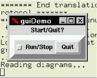
This small “widget” with two buttons, “Run/Stop” and “Quit” represents a simple dialog (see Fig. 1). Every time the user clicks the “Run/Stop” checkbutton, the script types to the standard output 0 or 1 (supposed to be swallowed by DIANA), depending on the state of the button, and reads the window header from the standard input. If the user clicks the “Quit” button, then the script outputs the line Quit to the standard output, and exits.

The script is started by means of the operator \pipe(./guiDemo) during initialization of a TM program:

\Begin(initialization)
   . . .
   \export(guiDemo,\pipe(./guiDemo))
   \topipe(\import(guiDemo),Start/Quit?\eol())
   \if"\frompipe(\import(guiDemo))"ne"1"then
      \exit(-1)
   \endif
   \topipe(\import(guiDemo),Run\( )0...\eol())
\End(initialization)

At this point the window appears with the title “Start/Quit?” (Fig. 1 a)) , and the execution of the TM program will be suspended since it is blocked while waiting for the data from the pipe.

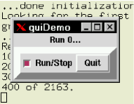
If the user clicks on the “Quit” button, the TM program will be finished. If the user switches on the “Run/Stop” button, the TM program starts to run (Fig. 1 b)).

Each time the user clicks one of the buttons (or closes the window), the script emits some text, which becomes available for \frompipe().

In the beginning of the “regular” section there is the following TM code:

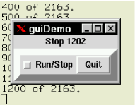
\section(regular)

\if"\ispipeready(\import(guiDemo))"eq"ok"then
\beginlabels
\label(_start)
\goto(_\frompipe(\import(guiDemo)))
\label(_0)
\topipe(\import(guiDemo),Stop\( )\currentdiagramnumber()\eol())
\goto(_start)
\label(_)
\label(_Quit)
\exit(-1)
\label(_1)
\topipe(\import(guiDemo),Run\( )\currentdiagramnumber()...\eol())
\endlabels
\endif

If the user switches off the “Run/Stop” button, this code suspends the execution of the TM program (Fig. 1 c)). The number of the current diagram will be typed into the title.

The user can continue (checking the “Run/Stop” button), or interrupt the TM program by means of the “Quit” button.

4 Running external commands asynchronously

4.1 Parallelization, local and remote jobs and synchronization

The operator \system() executes commands synchronously, i.e. it waits for them to be completed and returns an exit code. In contrast, the operator \_exec() executes commands in the background. Similar to the operator \pipe(), it does not wait for the command to be completed. It returns an empty string on success, or some diagnostics on failure. This operator may be used to parallelyze the evaluation of a process by running more than one job simultaneously.

All jobs started by the operator \_exec() are running independently of the TM program invoking them. To synchronize the TM program with all these jobs, there is an operator \_waitall(). It suspends execution of the TM program until timeout is expired, or until all jobs started by the \_exec() operator are completed (for further options see Sect. 4.3). It returns the number of jobs which are not yet finished, or an empty string, if there are no jobs anymore. The single argument of the operator \_waitall() is a timeout in milliseconds. E.g., \_waitall(1000) will return in one second the number of remaining jobs. If the user wants to know how many jobs are not yet finished, he may use the operator \_waitall(0).

To avoid overloading of a processor, by default at each time only one job is actually running while all the rest is waiting in the queue. The operator \_exec() just queues jobs.

On SMP computers, the optimal number of simultaneously running jobs is the number of processors. This number can be changed by means of the option -smp. Thus, -smp 8 tells DIANA to run on the computer 8 jobs simultaneously while all the rest is queued.

In case of a cluster of computers with a current directory shared by means of NFS e.g., the operator \_exec() can use DIANA servers running on other computers. To run DIANA as a server, the user may use one of the following two options: the option -s tells DIANA to run a server listening to some port, and the option -d forces DIANA to fork out a “daemon” running in the background and listening to the port instead of DIANA. Thus, each computer on which the user has executed the command (possibly automized, see macro STARTSERVERS below)

diana -d 1 -q

becomes available to perform the commands queued by the operator \_exec() (we assume that the current directory is shared by NFS among all computers in the cluster). Here -d 1 tells DIANA to run a daemon accepting only one connection, and the option -q terminates the father DIANA process. For SMP computers the optimal argument for the -d (or -s) option is the number of processors.

Running jobs are controlled by means of “handlers”. These can be understood as communication channels between running jobs and DIANA. Their number is the highest possible number of simultaneously running jobs. By default, the operator \_exec() will give priority to local handlers, i.e. if the two possibilities occur simultaneously to run a job locally or on a remote server, the job will be started on the local computer. When DIANA starts a new job, it tries to use one of the free handlers with minimal nice. The nice is an integer number which is set for each handler. By default, the local handler has nice 0, while the remote handler has nice 1.

The nice of local handlers can be set by an optional parameter for the option -smp, separated by a comma from the mandatory parameter. Thus, -smp 8 tells DIANA to run on the computer 8 jobs simultaneously with nice 0 while -smp 8,2 tells DIANA to run these 8 jobs with nice 2.

The same with the remote server: -d 2 (or -s 2) tells DIANA to run a daemon (server) accepting two connections with nice 1, and -d 2,0 (or -s 2,0) tells DIANA to run a daemon (server) accepting two connections with nice 0.

4.2 Job attributes and exact syntax of operators

Two operators \_exec() and _waitall() permit the user to organize a simple parallel session for evaluations on SMP computers and/or clusters of independent computers with shared disk space. But very often this is not enough (see Introduction). Therefore, each job started by the operator \_exec() must have further attributes (for a complete list see the end of the present section). The first one is the “sync” attribute; if it is set, the job will be started to run only after all previously started jobs are completed. The second attribute is the “sticky” attribute. This attribute requires a parameter, which gives reference to the “master” job to which the “slave” (getting this parameter) has to stick. If this attribute is set, the “slave” will be performed on the same node as the “master” job was running.

If the “master” job fails before the “sticky” “slave” job was started, the latter will fail too if a third attribute is set; otherwise it will be performed independently of the result of the “master” job. Let’s call this attribute “stickyfail”.

There are some other attributes, which will be explained further down. The total number of attributes is 32, but at present many of them are merely reserved for future developments.

The operator \_execattr(attr,param) is used to change default job attributes. attr is a string of length 32 in general. The position of each character corresponds to one of the attributes. The first character corresponds to the “sync” attribute, the second one to the “sticky” attribute, etc. If the corresponding character is 0, then the attribute is cleared, if 1, the attribute is set; any other character means that the attribute will not be changed. If the string attr is longer than 32, all extra characters will be ignored. If it is shorter, all remaining attributes will not be changed. Examples:

\_execattr(00000000000000000000000000000000,)

clears all attributes.

\_execattr(1,)

sets the “sync” attribute.

The second argument, param, is used to attach a parameter to attributes which require it. Parameters are attached consecutively only to those attributes which require them and only to attributes which are set. If more than one parameter is specified, they have to be separated by the end-of-file symbol (EOF), which can be obtained by the operator \eof(). If less parameters than set attributes are specified, they will be cycled over all set attributes requiring a parameter.

Each job started by \_exec() has a unique name, provided by the user (see below) or defined automatically. The parameter for sticky attributes is the name of the “master” job. It is not allowed to stick to jobs which are not yet queued. The name of the last queued job can be obtained by the operator \lastjobname(). So, the operator

\_execattr(!10,\lastjobname())

does not change the “sync” attribute, raises the “sticky” attribute to stick the new job to the job queued just before, and clears the “stickyfail” attribute.

Another example:

\_execattr(111,\lastjobname())

The newly created job will be executed firstly after the “master” job and all previously queued jobs are finished, secondly, on the same node on which the “master” job was performed, and thirdly only if the “master” job was successful.

If the parameter for the “sticky” attribute is an empty string, the last job name will be used and the above example is equivalent to

\_execattr(111,).

The operator \_exec() queues jobs defined by commands with arbitrary number of command line arguments. The command and the arguments must be pushed into a stack in natural order by means of the operator \push(). E.g., in order to execute a command “ls -l”, the user has to prepare the stack by means of the following set of operators:

\push(\eof())
\push(ls)
\push(-l)

and then invokes the operator \_exec(). The command line arguments appear in the stack in reverse order, reading from top to bottom, i.e. in the stack the EOF is situated on the bottom. The \_exec() operator reverses the command line arguments from the stack such that they appear in natural order again. The exact syntax of the \_exec() operator is as follows:

\_exec(name, attr, param).

Here name is the unique job name. If it is left empty, which is recommended in general, it will be assigned automatically.

The second and third argument have the same meaning as described above in connection with the \_execattr() operator. Here they are considered as local arguments and the default ones are not overwritten by the \_exec().

Besides these most important attributes we describe two more useful ones. They are “successcondition” and “restart”.

If the job is sent to a server, DIANA waits for an answer from it. The server reports success/failure of starting the job, and after the job is completed, the server reports the status of the job returned by the system.

By default, the job is assumed to be successful if the server reports the status. However, sometimes it is useful to investigate the status returned by the system, or assume that the job is successful if it is started by the server (see the discussion in the Introduction).

The “successcondition” attribute (the fourth one) can accept a parameter which can take the following values:

• -2 – the job is successful if it is started by the server;

• -1 – the same like without the attribute. The job is successful if the server reports the status returned by the system.

• from 0 to 255 – the job is successful if the external program initiated by the job has been completed and returned the exit code less or equal to the specified number.

Another problem with success/failure conditions is the question how many times the job should be restarted when it fails. By default, the job is not restarted at all on failure. To change this behaviour, a fifth attribute can be set. We call it the “restart” attribute. The corresponding parameter is the number of restarts, which must be an unsigned integer from 0 to 255.

Here is the synopsis of all attributes actually used by DIANA for the time being:

No	Attribute	Parameter
1	sync	–
2	sticky	job name (text)
3	stickyfail	–
4	successcondition	-2…255
5	restart	0…255

4.3 Related operators

As described in Sect. 4.1, the operator \_waitall() returns control if there are no more running jobs or if the timeout is expired. As third possibility the operator will return control if some data are available on a definite pipe. This pipe must be set by means of the operator \setpipeforwait(rpipe), where rpipe is the PID returned by the operator \pipe(), or 0. In the latter case the operator \_waitall() will return control if there is something typed on the keyboard.

If control is returned due to available data from the pipe, the number returned by the operator \_waitall() is preceded by a minus sign. If all jobs finish simultaneously with data occurring in the pipe only a minus sign is returned.

The operator \getpipeforwait() returns the PID of the pipe which has been set by \setpipeforwait(rpipe) or an empty string if there is no active pipe for \_waitall().

\pingServer(ip) checks if a DIANA server is available on a given IP address. The argument ip is the IP address in standard dot notation. The operator returns alive if the server responds, or an empty string if the server cannot be found or does not respond.

\killServer(ip) kills the DIANA server running on the specified IP address. The argument ip is again the IP address in standard dot notation. The operator returns ok on success, or an empty string on failure.

\killServers() kills all running DIANA servers. It returns an empty string on success, or none on failure.

\lastjobname() returns the name of the last job started by the operator \_exec().

\lastjobnumber() returns the number of the last job started by the operator \_exec().

\whichIP(jobname) returns the IP address as 8 hexadecimal digits or an empty string on failure.

\whichPID(jobname) returns the PID as a hexadecimal number or an empty string on failure.

\getnametostick(jobname) returns the name of the “master” job to which the specified “sticky” job jobname has to stick. On failure it returns an empty string.

\jobtime(jobname) returns 8 hexadecimal digits, the job running time in milliseconds. If the job is not yet running, the operator returns “00000000”.

\jobstime(jobname) returns 8 hexadecimal digits, the job starting time in milliseconds. The starting time is counted from the moment of the DIANA job queuing mechanism being activated till the time the job starts to run. If the job is not yet started, it returns “00000000”.

\jobftime(jobname) returns 8 hexadecimal digits, the job finishing time in milliseconds. The finishing time is counted from the moment of the DIANA job queuing mechanism being activated till the job is completed. If the job is not yet finished, it returns “00000000”.

\rmjob(jobname) removes the named job. If the job is running, the related external programs will automatically be killed by the signal SIGKILL. The operator returns an empty string independently of the result.

\clearjobs() clears all jobs. It returns an empty string on success, or the string “Client is dead.”

\jobstatus(jobname) returns the status of a specified job. The status is given in terms of 8 hexadecimal digits. The first two digits stand for the exit() argument of the external program if the program exited normally, otherwise they are “00”. The third and fourth digits are the following: “00” – normal exit, “01” – exit because of non-caught signal, “02” – the job was not run, “03” – no such job, “04” – job is finished, but its status is lost (often occurs after the debugger being detached); otherwise – “ff”. If the job was removed by the operator \rmjob(), the third digit will not be “0” but “1”.

The last 4 digits stand for the number of the signal that caused the external program to terminate if the fourth digit was “1”, otherwise “0000”.

\startjobtimeout(timeout) sets the timeout for attempts to start jobs (milliseconds). After the timeout is expired and the job is not yet running, it will be moved to another handler if the total number of the timeout hits is less then 10. If the number of timeout hits is 10, the job fails. Time is counted from the moment of the job being sent to the remote (or local) server. The operator returns the previous value of the timeout or an empty string on failure.

\gconnecttimeout() sets the timeout for the connection with a remote server (milliseconds). It returns the previous value of the timeout, or an empty string on failure.

\jobhits(jobname) returns 6 hexadecimal digits. The first two digits stand for the number of times the job was restarted due to the start timeout expiration. The third and fourth digits stand for the number of times the job was restarted after failures and the last two digits represent the current placement of the job: “01” – the job is in the main queue, “02” – the job is in the synchronous queue, “03” – the job is finished, “04” – the job failed, “05” – the job runs, “06” – the job is ready to run as a non-sticky job, “07” – the job is ready to run as a sticky job.

\failedN() returns number of failed jobs, or an empty string, on failure.

\hex2sig(sig) converts DIANA’s internal signals’ hexadecimal representation to local system ones (decimal numbers).

\sendsig(jobname,signal) sends a signal to the external program which was initiated by the specified job. Note, the signal will be sent to all external programs initiated by the job. It expects that the signal is either a symbolic name SIG… (the SIG prefix may be omitted), or a number. All possible symbolic names are (a subset from the conventional UNIX signal identifiers): SIGHUP SIGINT SIGQUIT SIGILL SIGABRT SIGFPE SIGKILL SIGSEGV SIGPIPE SIGALRM SIGTERM SIGUSR1 SIGUSR2 SIGCHLD SIGCONT SIGSTOP SIGTSTP SIGTTIN SIGTTOU SIGBUS SIGPOLL SIGPROF SIGSYS SIGTRAP SIGURG SIGVTALRM SIGXCPU SIGXFSZ SIGIOT SIGEMT SIGSTKFLT SIGIO SIGCLD SIGPWR SIGINFO SIGLOST SIGWINCH. If the signal is specified by a number, the signal will be sent as it is. If the signal is specified by a symbolic name, DIANA will convert it into an internal representation transferred to the remote server. This may be useful if the numerical representation of signals on the remote system differs from the local one. The operator returns an empty string on success; on failure it returns: “10” – job is not run, “20” – can’t read a signal from DIANA; less then 10: “01” – an invalid signal was specified, “02” – the pid or process group does not exist, “03” – the process does not have permission to send the signal, “04” – unknown error.

\getJobInfo(jobn, format) returns information about the job number jobn, formatted according to format. The latter is a string of type n1/w1:...:nn/wn’, where n# is a field number and w# is its width. If w#$\,\,>0$, the text in the field will be right justified and padded on the left with blanks. If w#$\,\,<0$, then the text in the field will be left justified and padded on the right with blanks. If w#=0, then the width of the field will be of the text length. Here is a complete list of all available fields:

1. current placement, see above;

2. return code, 8 hexadecimal digits, see above;

3. IP address (in dot notation);

4. PID (decimal number);

5. attributes (decimal integer);

6. timeout hits (decimal number), see above;

7. fail hits (decimal number), see above;

8. max fail hits (decimal number), see above;

9. errorlevel (decimal number), see above;

10. the job name;

11. number of command line arguments;

12. all command line arguments starting from a second one (spaces separated);

13. all command line arguments starting from a third one (spaces separated);

14. all command line arguments starting from a fourth one (spaces separated).

If n# is zero or negative its absolute value is interpreted as the position of a single command line argument.

Example: \getJobInfo(1, 4/10:3/15) returns the PID of the external program of the first job and the IP address of the computer on which the job runs. PID will be returned as a decimal number padded by spaces on the left to fit a field of width 10, and IP will be returned in dot notation padded by spaces on the left to fit a field of width 15.

\tracejobson(filename) starts jobs tracing (for details see
http://www.physik.uni-bielefeld.de/~tentukov/parallel_demo.tar.gz) into files (“filename.var” and “filename.nam”), returns an empty string.

\tracejobsoff() ceases tracing. It returns an empty string. After it has stopped, tracing cannot be continued until all jobs are cleared by means of the operator \clearjobs().

4.4 Example of high-level usage of parallel processing facilities

Very often the external program may run in a subshell as a conventional UNIX command. For such cases the following high-level TM function \exec(command) can be defined:

\function exec cmd;
 \push(\eof())
 \push(sh)
 \push(-c)
 \push(\get(cmd))
 \return(\_exec(,00011,255\eof()4))
\end

The function starts the job consisting of some (maybe composed) standard UNIX command. The job will be successful if the command returns some exit code (under UNIX there is no possibility to have an exit code higher then 255). On failure the job will be restarted up to four times (the number 4 after \eof()).

The function \stick(command):

\function stick cmd;
 \push(\eof())
 \push(sh)
 \push(-c)
 \push(\get(cmd))
 \return(\_exec(,11110,\eof()-2))
\end

performs the command cmd only after all earlier jobs are completed (the first 1 of the second argument of \exec()). This function in general is used to collect all produced files. That is why it performs cmd on the same computer as the preceding job (the second 1; since the job name to stick to is an empty string, the last job name will be used). The job started by this function is successful if it is started by the server (the fourth 1, and the corresponding parameter is “-2”). The job will not be restarted on failure (the last 0).

The function \wait(timeout):

\function wait to;
 \while"\let(r,\_waitall(\get(to)))"ne""do
  \message(\get(r)\( jobs are not finished))
 \loop
\end

suspends execution of the TM program until all jobs are completed. Each “timeout” milliseconds the function reports the number of jobs which are not yet finished.

These three functions can be used to organize a simple parallel session with proper synchronization. As an example, let us consider the following script runf, which is used to run FORM jobs in parallel after the FORM input has been produced in a folder (see [1], p. 158):

#!diana -smp 1 -c runpar.tml
\STARTSERVERS(phya25,phya26,phya27,phya28)
\system(echo > log.all)

\REPEAT(N)
\exec(form -d i=\get(N) do.frm > /tmp/log.\get(N))
\stick(cat /tmp/log.\get(N) >> log.all)
\stick(rm /tmp/log.\get(N))
\ENDREPEAT()

\wait(2000)

The user enters: runf 186 200 , and the system executes:
diana -smp 1 -c runpar.tml runf 186 200.

The file runpar.tml (see Appendix B) contains definitions of various TM functions and some settings; in particular it redefines the comment character as #. The following is the structure of the file runpar.tml:

messages disable
esc character = \
comment character = #
output file =""
debug off
only interpret
\begin translate

Definitions various functions and macros, in particular \exec(), \wait(),
\REPEAT(), \ENDREPEAT() and \STARTSERVERS()

\program
\-
\SET(_CMDLN)(\CMDLINE(1))
\RMARG(1)
\{\include(\GET(_CMDLN))\-
\setout(null)
\}
\end translate

The main program switches off the output (by means of the directive \-), switches off “hash” regime for arguments by means of the directive “\{” (see below), stores the first command line argument (“\SET(_CMDLN)(\CMDLINE(1))”), removes it (“\RMARG(1)”) and includes the file the name of which is the first command line argument
(“\include(\GET(_CMDLN))”).

By default, DIANA provides for the function and operator arguments some special “hash” regime: all spaces and ends of line are ignored. The directive “\{” cancels this regime, the directive “\}” activates it again. Without this directive all commands with spaces must be quoted by the quotation operator “\()” which is not convenient for a script.

The macro \STARTSERVERS(list) checks if each server from list is working and if not starts the server by means of the ssh. For example, for the host phya26 the following command will be performed:

ssh phya26 cd CD ; diana -d 1 -q

where “CD” is a current directory, e.g. /home/user/jobs.

The operator \system(echo > log.all) is used to produce an empty file “log.all”.

All the instructions between \REPEAT(N) ... \ENDREPEAT() are cycled with N=186,...,200. We assume that there is some folder file, say, tt.in with FORM input for each diagram. The FORM program do.frm evaluates a diagram by virtue of including a fold from the folder tt.in via an instruction like #include tt.in # n’i’. The macro definition i comes from the command line form -d i=\get(N) do.frm, where \get(N) runs from 186 to 200. Each FORM job saves the result to the local directory, but the corresponding concatenation is performed by \stick(cat ...) on the same computer. At the end, all results will be collected in the file log.all, and all intermediate files \tmp\log.# will be removed.

After all jobs are queued, the function \waitall(2000) will report every 2 seconds how many jobs are not yet completed.

This example is available at
http://www.physik.uni-bielefeld.de/~tentukov/parallel_demo.tar.gz.

In the archive there are two directories: demo1 and demo2. The example is situated in demo1; see the Readme file for details of installation. For a more realistic (and complicated) example containing jobs controlling and monitoring facilities see demo2.

Acknowlegement

M. Tentukov is grateful for financial suuport by the DFG under project no. FL 241/4-2

Appendix

Appendix A The listing of the Tcl/Tk script guiDemo

The following Tcl/Tk script is supposed to be placed into the executable file guiDemo:

#! /bin/sh
#\
exec wish "$0" "$@" -geometry +200+300

# catches destroy window event:
wm protocol .WM_DELETE_WINDOW {puts "Quit";exit 0}

label .title
pack .title

# create relief canvas:
frame .buttons -bd 10 -relief raised

#Button "Run/Stop":
global checkb
frame .buttons.run
checkbutton .buttons.run.run -text "Run/Stop"\
  -command {puts "$checkb"; flush stdout;\
            .title configure -text [gets stdin]}\
             -variable checkb
pack .buttons.run.run
pack .buttons.run -side left

#Button "Quit"
frame .buttons.quit
button .buttons.quit.quit -text "Quit" -command\
  {puts "Quit";exit 0}
pack .buttons.quit.quit
pack .buttons.quit -side left
pack .buttons

# Read initial header:
.title configure -text [gets stdin]
#End:

The script creates a window with two buttons. The check button “Run/Stop” has two states, “selected” and “deselected”. The global variable checkb is set to indicate whether or not this button is selected. Every time the user clicks the “Run/Stop” checkbutton, the script types to the standard output the value of checkb and reads the window header from the standard input. The “Quit” button, when pressed, outputs the line “Quit” to the standard output and exits from the script. The same occurs when the user closes the window.

Appendix B The listing of the file “runpar.tml”

The following listing is typed in typewriter while comments are typed using italic.

Preamble:
messages disable
esc character = \
comment character = #
output file =""
debug off
only interpret
\begin translate

The function returns  true if
the argument is a number:
\function isnumber str;
  \if"\get(str)"eq""then
     \let(res,)
  \else
     \let(sk,\getcheck())
     \setcheck(0123456789)
     \let(res,\check(\get(str)))
     \setcheck(\get(sk))
  \endif
  \return(\get(res))
\end

\function wait to;
 \while"\let(r,\_waitall(\get(to)))"ne""do
  \message(\get(r)\( jobs are not finished))
 \loop
\end

Begin macrodefinition of the
REPEAT environment
\DEF(REPEAT)
\IFSET(__REP)
\ERROR(Nested REPEAT!)
\ENDIF
\SET(__REP)(1)

Checking command line arguments:
\if"\exist(__From)"eq"false"then
   \let(__From,\cmdline(1))
\endif
\if"\exist(__To)"eq"false"then
   \let(__To,\cmdline(2))
\endif
\beginlabels
\label(again)
\while"\isnumber(\get(__From))"ne"true"do
   \let(__From,\read(’\get(__From)’
      \( is not an integer, enter new FROM:)))
\loop

\while"\isnumber(\get(__To))"ne"true"do
   \let(__To,\read(’\get(__To)’
      \( is not an integer, enter new TO:)))
\loop

\if"\numcmp(\get(__From),\get(__To))"eq">"then
   \message(\get(__From)>\get(__To)!)
   \let(__From,)\let(__To,)
   \goto(again)
\endif
\endlabels

 Pre-processor SCAN is used since macro argument \#(1)
 cannot be used in \if operator:
\SCAN(\if"\#(1)"eq""then)
   \let(_iND,_index) Default iterator
\else
   \let(_iND,\#(1)) Use argument as iterator
\endif

\let(\get(_iND),\get(__From))
\do  Start the main loop
\ENDDEF
End macrodefinition of the
REPEAT environment

Macrodefinition of the ENDREPEAT
environment, rather simple:
\DEF(ENDREPEAT)
End of the main loop
\while"\numcmp(\inc(\get(_iND),1),\get(__To))"ne">"loop
\UNSET(__REP)
\ENDDEF

\function exec cmd;
   \push(\eof())
   \push(sh)
   \push(-c)
   \push(\get(cmd))
  \return(\_exec(,00011,255\eof()4))
\end

\function stick cmd;
   \push(\eof())
   \push(sh)
   \push(-c)
   \push(\get(cmd))
   \return(\_exec(,11110,\eof()-2))
\end

Attention! The following macro assumes that
the executable file “diana” is availavle
from the system path set in the PATH variable,
and the current directory is shared by NFS:
\DEF(STARTSERVERS)
   \let(_cmd,\( ’cd )\asksystem(pwd,)\( ; diana -m d -d 1,1 -q’))
   \FOR(_srv)(\*) Loop on all arguments
     Remove possible spaces from the server name:
     \let(_n,\delete(\_srv(),\( )))
     \let(_ip,)
     \if"\get(_n)"ne""then
        Get IP address:
        \let(_ip,\getip(\get(_n)))
     \endif
     \if"\get(_ip)"ne""then
        Is the server alive?:
        \if"\pingServer(\get(_ip))"eq""then
           Not yet. Start it:
           \message(\(Starting server at )\get(_ip)...)
           \system(\(ssh )\get(_ip)\get(_cmd))
        \endif
     \endif
   \ENDFOR
  Servers may be started successfully, but
   network connection establishing may take some time.
   So try to ping servers, and if it does not respond,
   wait one second:
   \FOR(_srv)(\*)
     \let(_n,\delete(\_srv(),\( )))
     \let(_ip,)
     \if"\get(_n)"ne""then
        \let(_ip,\getip(\get(_n)))
     \endif
     \if"\get(_ip)"ne""then
        \if"\pingServer(\get(_ip))"eq""then
           \system(sleep 1)
        \endif
     \endif
   \ENDFOR
\ENDDEF

Main program:
\program
\- Switch off output
Store first command line argument:
\SET(_CMDLN)(\CMDLINE(1))
\RMARG(1)\ Remove it
Now command line arguments available
from the script are counted in correct order
Include a script body:
\{\include(\GET(_CMDLN))\-
Switch off output and close output
possibly opened by the script:
\setout(null)
\}
\killServers() Kill all servers
\end translate

References

- [1] J. A. M. Vermaseren, Symbolic manipulation with FORM (Amsterdam, Computer Algebra Nederland, 1991).
- [2] L. Avdeev, J. Fleischer, M. Y. Kalmykov, and M. Tentyukov, “Towards automatic analytic evaluation of massive Feynman diagrams”, Nucl. Instrum. Meth. A389 (1997) 343; L. V. Avdeev, J. Fleischer, M. Y. Kalmykov, and M. N. Tentyukov, “Towards automatic analytic evaluation of diagrams with masses”, Comput. Phys. Commun. 107 (1997) 155–166.
- [3] M. Tentyukov and J. Fleischer, “A Feynman diagram analyzer DIANA”, Comput. Phys. Commun. 132:124-141,2000, see also http://www.physik.uni-bielefeld.de/ tentukov/diana.html.
- [4] J. Fleischer et al., Phys. Lett. B459 (1999) 625; J. Fleischer, O. V. Tarasov and M. Tentyukov, Nucl. Phys. Proc. Suppl. 89 (2000) 112; F. Jegerlehner, M. Y. Kalmykov and O. Veretin, Nucl. Phys. B641 (2002) 285; J. Fleischer et al., hep-ph/0202109; A. Onishchenko and O. Veretin, hep-ph/0209010 and hep-ph/0211280; M. Awramik et al., hep-ph/0209084.
- [5] P. Nogueira, J. Comput. Phys. 105 (1993), 279.
- [6] Kaplan, J. A., Nelson M. L.: A Comparison of Queuing, Cluster and Distributed Computing Systems. Technical Report TM-109025, NASA Langley Research Center, June 1994.
- [7] C. Szyperski, Component Software, Beyond Object-Oriented Programming. Addison-Wesley, ACM Press, New York, 1998.