October 2003

Motivated by new precise results on several $K_{L}$ decays, sensitive to the ${K_{L}\to\gamma\gamma}$ form factor, we present a new analysis of the $K_{L}\to\mu^{+}\mu^{-}$ long-distance amplitude based on the semi-phenomenological approach of Ref. [1]. Particular attention is devoted to the evaluation of the uncertainties of this method and to the comparison with alternative approaches. Our main result is a conservative upper bound of $2.5\times 10^{-9}$ on $B(K_{L}\to\mu^{+}\mu^{-})_{\rm short}$, which is compatible with the SM expectation and which provides significant constraints on new-physics scenarios. The possibility to extract an independent short-distance information from future searches on $K_{S}\to\mu^{+}\mu^{-}$ is also briefly discussed.

1 Introduction

The rare decays $K_{L,S}\to\mu^{+}\mu^{-}$ are a very useful source of information on the short-distance structure of $\Delta S=1$ flavor-changing neutral-current (FCNC) transitions. In both cases the decay amplitude is not dominated by the clean short-distance contribution; however, long- and short-distance components are comparable in size. As a result, even with a limited knowledge of the long-distance component, it is possible to extract significant constraints on the short-distance part.

At present the $K_{L}\to\mu^{+}\mu^{-}$ decay is particularly interesting in this perspective because of the very precise determination of its decay rate [2]. Here the key issue to extract bounds on the short-distance amplitude is the theoretical control of the $K_{L}\to\gamma\gamma$ form factor with off-shell photons. An effective strategy to reach this goal is the combination of phenomenological constraints from $K_{L}\to\gamma\gamma$, $K_{L}\to\gamma\ell^{+}\ell^{-}$ and $K_{L}\to\mu^{+}\mu^{+}e^{+}e^{-}$ data, with theoretical constraints from chiral symmetry, large $N_{C}$, and perturbative QCD, proposed in Ref. [1]. As far as the phenomenological constraints are concerned, the situation has substantially improved in the last few years thanks to precise results on all the $K_{L}$ Dalitz modes [3, 4, 5] and, to a minor extent, because of the improvements on $K_{L}\to\gamma\gamma$ [6, 7]. On the theory side, alternative and/or complementary approaches about the high-energy constraints on the $K_{L}\to\gamma\gamma$ form factor have been discussed in Ref. [8, 9, 10, 11].

The main purpose of this paper is a new analysis of the $K_{L}\to\mu^{+}\mu^{-}$ two-photon dispersive amplitude, taking into account these new experimental and theoretical developments. In particular, as far as the theoretical constraints are concerned, we shall quantify the uncertainty of the method in Ref. [1] using a more general parameterization of the form factor. Moreover, we shall discuss in detail differences and similarities between this approach and the one of Ref. [8, 9]. As a result of this analysis, we find a conservative upper bound of $2.5\times 10^{-9}$ on $B(K_{L}\to\mu^{+}\mu^{-})_{\rm short}$, which is compatible with the SM expectation, $B(K_{L}\to\mu^{+}\mu^{-})^{\rm SM}_{\rm short}\approx 0.9\times 10^{-9}$, and which provides significant constraints on new-physics scenarios.

On the experimental side, the situation of the $K_{S}\to\mu^{+}\mu^{-}$ decay is very different with respect to the $K_{L}\to\mu^{+}\mu^{-}$ one: this process has not been observed yet, and present experimental limits are still very far from the SM expectation, $B(K_{S}\to\mu^{+}\mu^{-})^{\rm SM}\approx 5\times 10^{-12}$ [12]. On the theory side, the $K_{S}\to\mu^{+}\mu^{-}$ amplitude is particularly interesting since its short-distance component is dominated by the CP-violating part of the $s\to d\ell^{+}\ell^{-}$ amplitude, which is very sensitive to new physics and which is poorly constrained so far. As we shall show, future searches of $K_{S}\to\mu^{+}\mu^{-}$ in the $10^{-11}$ range, could provide significant constraints on several consistent new-physics scenarios.

The plan of the paper is as follows: in Section 2 we present the general decomposition of $K_{L}\to\mu^{+}\mu^{-}$ amplitude and branching ratio, and briefly review the structure of the short-distance component. In Section 3 we discuss the evaluation of the low-energy coupling $\chi_{\gamma\gamma}$, which encodes the information on the off-shell $K_{L}\to\gamma\gamma$ form factor; using this estimate, in Section 4 we analyse the present short-distance constraints from $K_{L}\to\mu^{+}\mu^{-}$. Section 5 is devoted to $K_{S}\to\mu^{+}\mu^{-}$. The results are summarized in the Conclusions.

2 Decomposition of the $K_{L}\to\mu^{+}\mu^{-}$ amplitude

2.1 General structure and experimental constraints

Within the Standard Model the $K_{L}\to\mu^{+}\mu^{-}$ decay is mediated by a CP-conserving $s$-wave amplitude which can simply be written as

$${\cal A}(K_{L}\to\mu^{+}\mu^{-})=\left(A_{\gamma\gamma}+{\rm Re}A_{\rm short}\right)\bar{\mu}\gamma_{5}\mu~{},$$ (1)

where $A_{\gamma\gamma}$ denotes the complex long-distance contribution generated by the two-photon exchange and ${\rm Re}A_{\rm short}$ the real amplitude of short-distance origin induced by $Z$-penguin and box diagrams (see Fig. 1). The long-distance amplitude has a large absorptive part (${\rm Im}A_{\gamma\gamma}$) which is completely dominated by the two-photon cut and provides the dominant contribution to the total $K_{L}\to\mu^{+}\mu^{-}$ rate. It is then convenient to normalize $\Gamma(K_{L}\to\mu^{+}\mu^{-})$ to $\Gamma(K_{L}\to\gamma\gamma)$ and decompose it as follows [8, 10]

$$\Gamma(K_{L}\to\mu^{+}\mu^{-}) = \frac{2\alpha_{\rm em}^{2}r_{\mu}\beta_{\mu}}{\pi^{2}}\left[R_{\rm abs}+R_{\rm disp}\right]\Gamma(K_{L}\to\gamma\gamma)~{},$$ (2)

$$R_{\rm abs} = ({\rm Im}C_{\gamma\gamma})^{2}=\left[\frac{\pi}{2\beta_{\mu}}\ln\frac{1-\beta_{\mu}}{1+\beta_{\mu}}\right]^{2}~{},$$ (3)

$$R_{\rm disp} = \left[\chi(\mu)-\frac{5}{2}+\frac{3}{2}\ln\left(\frac{m_{\mu}^{2}}{\mu^{2}}\right)+{\rm Re}C_{\gamma\gamma}\right]^{2}~{},$$ (4)

where $r_{\mu}=m_{\mu}^{2}/m_{K}^{2}$, $\beta_{\mu}=\sqrt{1-4r_{\mu}}$ and

$$C_{\gamma\gamma}=\frac{1}{\beta_{\mu}}\left[{\rm Li}_{2}\left(\frac{\beta_{\mu}-1}{\beta_{\mu}+1}\right)+\frac{\pi^{2}}{3}+\frac{1}{4}\ln^{2}\left(\frac{\beta_{\mu}-1}{\beta_{\mu}+1}\right)\right]~{}.$$ (5)

The real coupling $\chi(\mu)=\chi_{\rm short}+\chi_{\gamma\gamma}(\mu)$ encodes both short- and long-distance contributions: $\chi_{\rm short}$ denotes the genuine short-distance (scale-independent) contribution of the diagrams in Fig. 1b; $\chi_{\gamma\gamma}(\mu)$ is a low-energy effective coupling — determined by the behavior of the $K_{L}\to\gamma\gamma$ form factor outside the physical region — which compensates the scale dependence of the diagram in Fig. 1a (computed with a point-like form factor and regularized in the $\overline{MS}$ scheme).

The smallness of the total dispersive amplitude is well established thanks to precise experimental results on both $\Gamma(K_{L}\to\mu^{+}\mu^{-})$ and $\Gamma(K_{L}\to\gamma\gamma)$. As pointed out by Littenberg [16], we can minimize the experimental error on the ratio $\Gamma_{L}(\mu^{+}\mu^{-})/\Gamma_{L}(\gamma\gamma)$ decomposing it as the product of $\Gamma_{L}(\mu^{+}\mu^{-})/\Gamma_{L}(\pi^{+}\pi^{-})=(3.48\pm 0.05)\times 10^{-6}$ [2] times $\Gamma_{L}(\pi^{+}\pi^{-})/\Gamma_{L}(\gamma\gamma)$. The latter can in turn be determined as follows

$$\frac{\Gamma_{L}(\gamma\gamma)}{\Gamma_{L}(\pi^{+}\pi^{-})}=\left\{\begin{array}[]{lcl}\frac{\Gamma_{L}(\gamma\gamma)}{\Gamma_{L}(\pi^{0}\pi^{0})}\times\frac{\Gamma_{L}(\pi^{0}\pi^{0})}{\Gamma_{L}(\pi^{+}\pi^{-})}&=&0.2798\pm 0.0044~{}\cite[cite]{[\@@bibref{}{litt}{}{}]}\\ &&\\ \frac{\Gamma_{L}(\gamma\gamma)}{\Gamma_{L}(3\pi^{0})}\times\frac{\Gamma_{L}(3\pi^{0})}{\Gamma_{L}(\pi^{+}\pi^{-})}&=&0.2836\pm 0.0060\end{array}\right\}=0.2811\pm 0.0035~{},$$ (6)

where, in the second case, we have used $\Gamma_{L}(\gamma\gamma)/\Gamma_{L}(3\pi^{0})=(2.805\pm 0.018)\times 10^{-3}$ from the average of NA48 [6] and KLOE [7] recent results and $\Gamma_{L}(\pi^{+}\pi^{-})/\Gamma_{L}(3\pi^{0})=(9.89\pm 0.20)\times 10^{-3}$ from PDG [17]. The combination of the two ratios leads to

$$\frac{\Gamma(K_{L}\to\mu^{+}\mu^{-})}{\Gamma(K_{L}\to\gamma\gamma)}=(1.238\pm 0.024)\times 10^{-5}~{}.$$ (7)

According to Eqs. (2)–(4) this implies

$$R_{\rm disp}=\left[\chi_{\gamma\gamma}(M_{\rho})+\chi_{\rm short}-5.12\right]^{2}=0.98\pm 0.55\qquad{\rm or}\qquad R_{\rm disp}<1.7\ {\rm at}\ 90\%\ {\rm CL}~{},$$ (8)

to be compared with $R_{\rm abs}=27.14$ .

2.2 The short-distance component

Within the Standard Model (SM) the short-distance $K_{L}\to\mu^{+}\mu^{-}$ amplitude can be predicted with excellent accuracy in terms of the Cabibbo-Kobayashi-Maskawa (CKM) matrix elements $V_{ij}$. Following the notation of [14], we find

$${\rm Re}A^{\rm SM}_{\rm short}=-\frac{G_{F}\alpha_{\rm em}(M_{Z})}{\pi\sin^{2}\theta_{W}}\sqrt{2}m_{\mu}F_{K}\left[{\rm Re}(V_{ts}^{*}V_{td})Y(x_{t})+{\rm Re}(V_{cs}^{*}V_{cd})Y_{NL}\right]~{}.$$ (9)

Employing the decomposition (2)–(4) this leads to

$$\chi^{\rm SM}_{\rm short} = \kappa\left[\frac{-{\rm Re}(V_{ts}^{*}V_{td})Y(x_{t})-{\rm Re}(V_{cs}^{*}V_{cd})Y_{NL}}{4\times 10^{-4}}\right]=\kappa(1.11-0.92\bar{\rho})~{},$$ (10)

$$|\kappa| = 4\times 10^{-4}\left[\frac{m_{K}}{16\pi\Gamma(K_{L}\to\gamma\gamma)}\right]^{1/2}\frac{\sqrt{2}G_{F}m_{K}F_{K}\alpha_{\rm em}(M_{Z})}{\sin^{2}\theta_{W}\alpha_{\rm em}}=1.96~{},$$ (11)

where the second identity in (10) has been derived using the modified Wolfenstein parameterization of the CKM matrix [15] and the numerical estimates of $|V_{cb}|$ and $|V_{us}|$ from Ref. [15] (the two coefficients in Eq. (10) are affected by a $\sim 5\%$ error, mainly due to the uncertainty on $|V_{cb}|$ and $Y_{NL}$). Note that, as explicitly indicated, the value of $\alpha$ in the short-distance amplitude refers to the electromagnetic coupling renormalized at high scales $[\alpha_{\rm em}(M_{Z})=1/128]$, while in the long-distance part of the amplitude we use $\alpha_{\rm em}=1/137.036$ .

Within several SM extensions, the $K_{L}\to\mu^{+}\mu^{-}$ amplitude receives additional short-distance contributions which compete, in magnitude, with the SM one. With the exception of rather exotic scenarios, these new effects induce only a redefinition of $\chi_{\rm short}$. This happens, in particular, in the wide class of models where the dominant non-standard effects can be encoded in effective FCNC couplings of the $Z$ boson: a well-motivated framework [18, 19] with renewed phenomenological interest [20]. Following the notation of Ref. [19], here one can write

$$\chi_{\rm short}\ =\ \chi^{\rm SM}_{\rm short}-\kappa\frac{{\rm Re}\left(Z_{ds}-Z_{ds}^{\rm SM}\right)}{4\times 10^{-4}}~{},$$ (12)

where $Z_{ds}^{\rm SM}=C_{0}(x_{t})V_{ts}^{*}V_{td}$ and $C_{0}(x_{t})=0.79$.

a)

b)

Figure 1: Leading long-distance (a) and short-distance (b) contributions to $K_{L}\to\mu^{+}\mu^{-}$.

3 Theoretical estimate of $\chi_{\gamma\gamma}(\mu)$

3.1 The $K_{L}\to\gamma\gamma$ form factor

The necessary ingredient to estimate the low-energy coupling $\chi_{\gamma\gamma}(\mu)$ is the $K_{L}\to\gamma\gamma$ form factor, $f(q_{1}^{2},q_{2}^{2})$, defined by the four-point Green’s function

$$\int d^{4}xe^{iq_{1}x}\int d^{4}ye^{iq_{2}y}\langle 0|T\left\{J^{\mu}_{\rm em}(x)J^{\nu}_{\rm em}(y){\cal L}_{\Delta S=1}(0)\right\}|K_{L}\rangle\propto\epsilon^{\mu\nu\rho\sigma}q_{1\rho}q_{2\sigma}f(q_{1}^{2},q_{2}^{2})$$ (13)

and normalized such that $f(0,0)=1$. In terms of this form factor the $K_{L}\to\gamma\gamma$ vertex of Fig. 1 is written as

$${\cal A}\left[K_{L}\to\gamma(\varepsilon_{1},q_{1})\gamma(\varepsilon_{2},q_{2})\right]=i\frac{{\cal N}}{m_{K}}f(q_{1}^{2},q_{2}^{2})\epsilon_{\mu\nu\rho\sigma}\varepsilon_{1}^{\mu}\varepsilon_{2}^{\nu}q_{1}^{\rho}q_{2}^{\sigma}~{},$$ (14)

with ${\cal N}=[64\pi\Gamma(K_{L}\to\gamma\gamma)/m_{K}]^{1/2}=1.74\times 10^{-9}$, and

$$\chi_{\gamma\gamma}(\mu)=\left\{\frac{32\pi^{2}i}{q^{2}}\int\frac{d^{d}k}{(4\pi)^{d}}\frac{[q^{2}k^{2}-(q\cdot k)^{2}][f(k^{2},(k-q)^{2})-1]}{k^{2}(k-q)^{2}[(k-p)^{2}-m_{\mu}^{2}]}\right\}_{\overline{MS}}$$ (15)

with $q^{2}=m_{K}^{2}$ and $p^{2}=m_{\mu}^{2}$. As can be understood from Eq. (15), the leading contribution to $\chi_{\gamma\gamma}(\mu)$ in the chiral expansion (or in the limit where we neglect external momenta) is governed by $f(-k_{E}^{2},-k_{E}^{2})/k_{E}^{2}$, with $k_{E}^{2}\in[0,\infty]$.

The structure of $f(q_{1}^{2},q_{2}^{2})$ has been investigated by several authors (see e.g. Ref. [1, 8, 9, 10, 11, 21]). The general properties dictated by QED and QCD can be summarized as follows:

1. it is symmetric under the exchange $q_{1}^{2}\leftrightarrow q_{2}^{2}$;

2. it is analytic but for cuts and poles in the region $q_{1,2}^{2}>4m_{\pi}^{2}$, corresponding to the physical thresholds in the photon propagators;

3. the high-energy behavior in the Euclidean region is given by $f(-k_{E}^{2},-k_{E}^{2})\sim 1/k_{E}^{2}$ (up to logarithmic corrections).

Note that not all the parameterizations proposed in the literature satisfy these conditions. In particular, the properties ii. and iii. are not fulfilled by some of the parameterizations of Ref. [11]: this is one of the main reasons why we do not agree with the conclusions of this work.

In addition to these general properties, a systematic and powerful approach which leads to tight constraints on the structure of $f(q_{1}^{2},q_{2}^{2})$ is provided by the large $N_{C}$ expansion [8]. At the lowest order in $1/N_{C}$ we expect

$$f(q_{1}^{2},q_{2}^{2})=\sum_{i}\left[1+\alpha_{i}\left(\frac{q_{1}^{2}}{q_{1}^{2}-M_{i}^{2}}+\frac{q_{2}^{2}}{q_{2}^{2}-M_{i}^{2}}\right)+\beta_{i}\frac{q_{1}^{2}q_{2}^{2}}{(q_{1}^{2}-M_{i}^{2})(q_{2}^{2}-M_{i}^{2})}\right]~{},\qquad$$ (16)

$${\rm with}\quad\sum_{i}\left[1+2\alpha_{i}+\beta_{i}\right]=0~{},$$ (17)

where the sum extends over an infinite series of (infinitely narrow) vector-meson resonances and the sum-rule (17) follows from the $k_{E}^{2}\to\infty$ condition [8]. This type of structure is certainly not exact point-by-point in $q^{2}$, but it has been shown to provide an excellent tool to evaluate dispersive integrals of the type (15), even when the sum is truncated to the first non-trivial term (see e.g. Ref. [8, 22]). The truncation to the lowest vector-meson resonance (the $\rho$ meson) of Eq. (16) corresponds to the DIP ansatz [1] (with $\beta=-1-2\alpha$) and also to the choice of Ref. [9]. Within such approximation, the form factor depends on a single parameter: in the DIP case this is fixed at low energies by the experimental constraints on $df(q^{2},0)/dq^{2}$, while in Ref. [8, 9] the free parameter is determined by the OPE, matching the coefficient of the $1/k_{E}^{2}$ term for $k_{E}^{2}\to\infty$. In the case of pure electromagnetic decays, such as $\pi^{0}\to e^{+}e^{-}$ and $\eta\to\ell^{+}\ell^{-}$, these two procedures lead to almost equivalent results. On the contrary, in the case of $K_{L}\to\mu^{+}\mu^{-}$ these two approaches lead to a significant numerical difference. Once we assume the convergence condition $f(-k_{E}^{2},-k_{E}^{2})\sim 1/k_{E}^{2}$, the largest contribution to the integral (15) arises by the low-energy region. For this reason, we believe that the experimental determination of $df(q^{2},0)/dq^{2}$, at low $q^{2}$, provides the most significant constraint on $\chi_{\gamma\gamma}(\mu)$. However, in order to quote a reliable error on this quantity, we need to estimate also the sensitivity of the dispersive integral to the high-energy modes. To this purpose, in the following we shall employ a more general parameterization than the DIP ansatz, but still inspired by the $1/N_{C}$ expansion, namely

$$f(q_{1}^{2},q_{2}^{2}) = 1+\alpha\left(\frac{q_{1}^{2}}{q_{1}^{2}-M_{\rho}^{2}}+\frac{q_{2}^{2}}{q_{2}^{2}-M_{\rho}^{2}}\right)-(1+2\alpha-\delta)\frac{q_{1}^{2}q_{2}^{2}}{(q_{1}^{2}-M_{\rho}^{2})(q_{2}^{2}-M_{\rho}^{2})}$$ (18)

$$+\gamma\left(\frac{q_{1}^{2}}{q_{1}^{2}-\Lambda_{H}^{2}}+\frac{q_{2}^{2}}{q_{2}^{2}-\Lambda_{H}^{2}}\right)-(2\gamma+\delta)\frac{q_{1}^{2}q_{2}^{2}}{(q_{1}^{2}-\Lambda_{H}^{2})(q_{2}^{2}-\Lambda_{H}^{2})}~{},$$

with $\Lambda_{H}>M_{\rho}$. The choice of the four coefficients in (18) is such that the sum-rule (17) is automatically satisfied and for $\gamma=\delta=0$ we recover the DIP case (with $\beta=-1-2\alpha$).

The expression of $\chi_{\gamma\gamma}(\mu)$ obtained by means of the parameterization (18) is

$$\chi_{\gamma\gamma}(\mu)=\frac{3}{2}\ln\left(\frac{\mu^{2}}{M^{2}_{\rho}}\right)-R(M^{2}_{\rho},M^{2}_{\rho})+2\alpha\left[R(M^{2}_{\rho},0)-R(M^{2}_{\rho},M^{2}_{\rho})\right]$$

$$\qquad+\delta\left[R(M^{2}_{\rho},M^{2}_{\rho})-R(\Lambda_{H}^{2},\Lambda_{H}^{2})\right]+2\gamma\left[R(\Lambda_{H}^{2},0)-R(\Lambda_{H}^{2},\Lambda_{H}^{2})\right]~{},\quad$$ (19)

where, expanding up to the next-to-leading order in the chiral expansion,

$$\!\!\!\!R(M^{2},0)=-\frac{3}{2}\ln\left(\frac{M^{2}_{\rho}}{M^{2}}\right)-\frac{3}{2}+\frac{m_{K}^{2}}{M^{2}}\left[\frac{1-10r_{\mu}}{6}\ln\left(\frac{m_{\mu}^{2}}{M^{2}}\right)-\frac{11+34r_{\mu}}{36}\right]+{\cal O}\left(\frac{m_{K}^{4}}{M^{4}}\right)~{},$$

$$\!\!\!\!R(M^{2},M^{2})=-\frac{3}{2}\ln\left(\frac{M^{2}_{\rho}}{M^{2}}\right)-\frac{m_{K}^{2}}{M^{2}}\frac{1-5r_{\mu}}{3}+{\cal O}\left(\frac{m_{K}^{4}}{M^{4}}\right)~{}.$$ (20)

The result for $\chi_{\gamma\gamma}(\mu)$ in (19) depends on four free parameters: $\alpha$, $\gamma$, $\delta$ and $\Lambda_{H}^{2}$. As anticipated, one combination is fixed by the model-independent constraint following by the experimental measurement of the form factor in the Dalitz decays $K_{L}\to\gamma\ell^{+}\ell^{-}$ and $K_{L}\to e^{+}e^{-}\mu^{+}\mu^{-}$. The KTeV collaboration has performed a detailed analysis of this form factor, taking into account the significant distortions of the spectrum induced by radiative corrections [23]. As a result, a coherent determination of the slope

$$\alpha_{\rm exp}=-M^{2}_{\rho}\left.\frac{d}{dq^{2}}f(q^{2},0)\right|_{q^{2}=0}=\alpha+\frac{M_{\rho}^{2}}{\Lambda_{H}^{2}}\gamma$$ (21)

emerges from all the available channels: $K_{L}\to\gamma e^{+}e^{-}$ ($\alpha_{\rm exp}|_{ee}=-1.63\pm 0.05$ [5]), $K_{L}\to\gamma\mu^{+}\mu^{-}$ ($\alpha_{\rm exp}|_{\mu\mu}=-1.54\pm 0.10$ [3]), and $K_{L}\to e^{+}e^{-}\mu^{+}\mu^{-}$ ($\alpha_{\rm exp}|_{ee\mu\mu}=-1.59\pm 0.37$ [4]). Combining these results, we obtain the very precise value $\alpha_{\rm exp}=-1.611\pm 0.044$. Note that the consistency of the DIP parameterization for the various modes, as well as the one of the BMS model [21], provides a good support in favor of a generic VMD structure, such as the one in Eq. (18), with a minor role played by the terms associated to the heavier poles.

Taking advantage of the relation (21) and expanding up to the first order in the three small ratios $m_{\mu}^{2}/m_{K}^{2}$, $m_{K}^{2}/M_{\rho}^{2}$ and $M_{\rho}^{2}/\Lambda_{H}^{2}$, we can write

$$\chi_{\gamma\gamma}(M_{\rho}) = -3\alpha_{\rm exp}+\frac{m_{K}^{2}}{M^{2}_{\rho}}\left[\frac{1}{3}+\alpha_{\rm exp}\frac{1+6\ln(m^{2}_{\mu}/M_{\rho}^{2})}{18}\right]-\Delta_{\Lambda}=(5.83\pm 0.15)-\Delta_{\Lambda}~{},\quad$$

$$\Delta_{\Lambda} = \left[3\gamma\left(1-\frac{M_{\rho}^{2}}{\Lambda_{H}^{2}}\right)+\delta\left(\frac{m^{2}_{K}}{3M_{\rho}^{2}}-\frac{3}{2}\ln\frac{M_{\rho}^{2}}{\Lambda_{H}^{2}}\right)\right]~{}.$$ (22)

From the expression (22) we deduce that: i) $\chi_{\gamma\gamma}(M_{\rho})$ shows a rapid convergence in the chiral expansion; ii) the combination of $\gamma$, $\delta$ and $\Lambda_{H}^{2}$ which controls the sensitivity to the high-energy modes is $\Delta_{\Lambda}$. We also note that $\Delta_{\Lambda}\ll 1$ in the limit $\Lambda_{H}\to M_{\rho}$ ($\gamma$ and $\delta$ are expected to be at most of ${\cal O}(1)$ by naturalness arguments), thus the scenario which maximizes the sensitivity to high scales is the case $\Lambda_{H}^{2}\gg M^{2}_{\rho}$. Since charm loops play an important role in determining the short-distance behavior of this form factor, we cannot exclude a priori that $\Lambda_{H}$ is connected to the charm scale. For this reason, in the following we shall allow $\Lambda_{H}^{2}$ to reach values up to $10M^{2}_{\rho}$.

Estimates of $\Delta_{\Lambda}$ can be obtained by looking at the $k_{E}^{2}\to\infty$ behavior of $f(-k_{E}^{2},-k_{E}^{2})$:

$$\lim_{k_{E}^{2}\to\infty}f(-k_{E}^{2},-k_{E}^{2})=\frac{2}{k_{E}^{2}}\left[(1+\alpha-\delta)M_{\rho}^{2}+(\gamma+\delta)\Lambda_{H}^{2}\right]\doteq{\cal C}_{0}\frac{M_{\rho}^{2}}{k_{E}^{2}}~{}.$$ (23)

If $|{\cal C}_{0}|\stackrel{{\scriptstyle<}}{{{}_{\sim}}}1$, as it happens in the case of the pure electromagnetic form factors relevant to $\pi^{0}(\eta)\to\ell^{+}\ell^{-}$ decays [8], we must impose the condition $\gamma\approx-\delta$. As a first qualitative observation, we note that $\Delta_{\Lambda}$ is rather small once this condition is fulfilled: $|\Delta_{\Lambda}|<1$ for $\Lambda_{H}^{2}/M^{2}_{\rho}<10$ and $|\gamma,\delta|<1$. A more quantitative estimate along this line can be obtained following Ref. [9]: bosonizing the partonic currents in (13), Greynat and de Rafael argued that ${\cal C}_{0}$ can be computed explicitly to leading order in both the $1/N_{C}$ and the chiral expansion, obtaining

$${\cal C}_{0}=\frac{8\pi^{2}F_{\pi}^{2}}{N_{C}M^{2}_{\rho}}\left[1\pm{\cal O}(L_{5})\right]=0.38\pm 0.12~{}\cite[cite]{[\@@bibref{}{Greynat}{}{}]}~{}.$$ (24)

Using this constraint in (23) and imposing the additional conditions $|\gamma,\delta|<0.5$ and $2<\Lambda_{H}^{2}/M^{2}_{\rho}<10$, we find $\Delta_{\Lambda}=0.3\pm 0.6$, where the error scales almost linearly with the upper bound on $|\gamma,\delta|$ . This result already provides a good support in favor of the smallness of $|\Delta_{\Lambda}|$; however, we believe that an even more convincing argument can be obtained by looking at the partonic evaluation of $f(q_{1}^{2},q_{2}^{2})$, which we shall discuss in the following.

3.2 High-energy behavior of the $K_{L}\to\gamma\gamma$ form factor from perturbative QCD

In the Euclidean region of large $|q^{2}_{1,2}|$, with $|q^{2}_{1}-q^{2}_{2}|\gg\Lambda^{2}_{QCD}$, the $K_{L}\to\gamma\gamma$ form factor can computed reliably using perturbative QCD. Indeed, this kinematical configuration resembles the case of a heavy-quark decay into a two-body heavy-light system. Here non-perturbative effects associated to the hadronization of the external quark lines have shown to be factorizable — up to power suppressed terms — into appropriate hadronic wave functions [24]. We expect a similar factorization mechanism to hold also for the Green’s function in (13), where the lowest-order partonic kernel corresponds to the diagrams in Fig. 2, and the leading hadronic matrix element involved is simply

$$\langle 0|\bar{s}\gamma_{\mu}\gamma_{5}d|K^{0}(p)\rangle=i\sqrt{2}F_{K}p^{\mu}~{}.$$ (25)

a)                                          b)                                    c)

Figure 2: Lowest-order partonic diagrams contributing to the $K_{L}\to\gamma\gamma$ amplitude.

The $K_{L}\to\gamma\gamma$ amplitude computed in this way, at the leading-logarithmic level of accuracy, can be written as

$${\cal A}\left[K_{L}\to\gamma(\varepsilon_{1},q_{1})\gamma(\varepsilon_{2},q_{2})\right] = i\epsilon_{\mu\nu\rho\sigma}\varepsilon_{1}^{\mu}\varepsilon_{2}^{\nu}q_{1}^{\rho}q_{2}^{\sigma}\frac{16\alpha_{\rm em}G_{F}V_{us}^{*}V_{ud}F_{K}}{9\pi\sqrt{2}}\left[C_{2}(\mu)+3C_{1}(\mu)\right]$$ (26)

$$\times\left[I\left(\frac{q_{1}^{2}}{m_{c}^{2}},\frac{q_{2}^{2}}{m_{c}^{2}}\right)+T\left(\frac{q_{1}^{2}}{m_{c}^{2}}\right)+T\left(\frac{q_{2}^{2}}{m_{c}^{2}}\right)\right]~{},\qquad\quad$$

where $C_{1,2}(\mu)$ are the Wilson coefficients of the $\Delta S=1$ effective Hamiltonian, in the notation of Ref. [14], and

$$I(r_{1},r_{2}) = \frac{1}{6}+\int_{0}^{1}dx\int_{0}^{1-x}dy\left\{\frac{(2-x-y)+(r_{1}x+r_{2}y)(1-x-y)^{2}}{1-(r_{1}x+r_{2}y)(1-x-y)}\right.$$

$$\left.-(2-3x-3y)\ln\left[\frac{(r_{1}x+r_{2}y)(1-x-y)-1}{(r_{1}x+r_{2}y)(1-x-y)}\right]\right\}~{},\quad$$

$$T(r) = 2\int_{0}^{1}dx~{}x(1-x)\ln\left[\frac{rx(1-x)-1}{rx(1-x)}\right]~{}.\qquad$$ (27)

The Wilson coefficients $C_{1,2}(\mu)$ are understood to be computed at the leading-logarithmic level at $\mu\sim(q_{1}^{2}+q_{2}^{2})/2$, starting from the initial conditions $C_{2}(M_{W})=1$ and ${C_{1}(M_{W})=0}$.

In the limit $r_{1,2}\to-\infty$ we find

$$I(-r_{1},-r_{2}) \longrightarrow \frac{\ln[2(r_{1}+r_{2})]}{r_{1}+r_{2}}\left[1+{\cal O}\left(\frac{(r_{1}-r_{2})^{2}}{(r_{1}+r_{2})^{2}}\right)\right]~{},$$

$$T(-r_{1})+T(-r_{2}) \longrightarrow \frac{1}{r_{1}+r_{2}}\left[1+{\cal O}\left(\frac{(r_{1}-r_{2})^{2}}{(r_{1}+r_{2})^{2}}\right)\right]~{},$$ (28)

which agree with the results obtained in Ref. [1] in the limit $q_{1}^{2}=q^{2}_{2}$. On general grounds, the perturbative calculation is not reliable in the limit $q_{1}^{2}=q_{2}^{2}$, since this kinematical configuration leads to a soft-momentum kaon. This is indeed one of the main criticism which could be addressed to the DIP analysis. However, by means of Eqs. (28) we can now show that the limit $q_{1}^{2}=q_{2}^{2}$ does not spoil the leading $1/q_{1,2}^{2}$ behavior in the perturbative region $|q^{2}_{1}+q^{2}_{2}|\gg|q^{2}_{1}-q^{2}_{2}|\gg\Lambda^{2}_{QCD}$. For this reason, we shall use the perturbative result in (26), in the limit $-q_{1}^{2}=-q_{2}^{2}=k_{E}^{2}\gg\Lambda^{2}_{QCD}$, to constrain the high-energy behavior of $f(-k_{E}^{2},-k_{E}^{2})$.

The comparison of the perturbative form factor with the phenomenological parameterization, in the Euclidean region, is shown in Fig. 3. As can be noted, with a suitable choice of parameters it is quite easy to reproduce the perturbative behavior, at large $k_{E}^{2}$, with the phenomenological ansatz. In order to define a range of $\gamma$, $\delta$ and $\Lambda_{H}$ compatible with the high-energy behavior, we have imposed the condition that the phenomenological form factor must be in the range defined by the perturbative result, with or without QCD corrections, for $\sqrt{k_{E}^{2}}\geq 2$ GeV. This condition leaves a considerable uncertainty in the form factor in the region 1 GeV $\stackrel{{\scriptstyle<}}{{{}_{\sim}}}\sqrt{k_{E}^{2}}\stackrel{{\scriptstyle<}}{{{}_{\sim}}}4$ GeV (see Fig. 3). However, the resulting range for the weighted integral in (15) is rather limited. This fact should not surprise, since the kernel in (15) enhances the sensitivity to the low-energy region. As a result of this condition, we find

$$|\Delta_{\Lambda}|\leq 1.0~{}.$$ (29)

in good agreement with the conclusions already derived starting from Eqs. (23) and (24).

$f(-k^{2},-k^{2})$

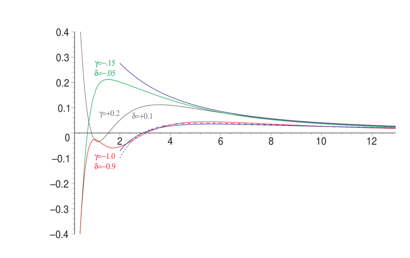
$\sqrt{k^{2}}$ (GeV)

Figure 3: Comparison of the perturbative form factor [lines starting from $\sqrt{k^{2}}=2$ GeV: upper full curve = no QCD corrections and un-expanded loop functions in Eq. (27); lower full curve = leading-log QCD corrections included and un-expanded loop functions; lower dotted curve = leading-log QCD corrections included and expanded loop functions in Eq. (28)] with the phenomenological ansatz, for $\Lambda_{H}=3~{}{\rm GeV}$ and different choices of the parameters (see text).

3.3 Interference of short- and long-distance components

As can be noted from Fig. 3, the short-distance constraint on $f(-k_{E}^{2},-k_{E}^{2})$ is not sufficient to determine the sign of the physical $K_{L}\to\gamma\gamma$ amplitude, or the sign of the coupling ${\cal N}$ in Eq. (14). By construction, we have assumed ${\cal N}>0$ in the phenomenological analysis, hiding this ambiguity in the sign of $\kappa$, the parameter of Eq. (10) which controls the interference between $\chi_{\gamma\gamma}(\mu)$ and $\chi_{\rm short}$.

Within Chiral Perturbation Theory, the leading contributions to the on-shell $K_{L}\to\gamma\gamma$ amplitude are the tree-level pole diagrams with $\pi^{0}$, $\eta$ and $\eta^{\prime}$ exchange [28]. In all realistic scenarios of pseudoscalar meson mixing, the contributions induced by $\eta$ and $\eta^{\prime}$ poles cancel to a large extent and the $K_{L}\to\gamma\gamma$ amplitude turns out to be dominated by the $\pi^{0}$ pole (see e.g. Ref. [7, 10, 28]). The $\pi^{0}$ pole contribution to the $K_{L}\to\gamma\gamma$ amplitude can be written as

$${\cal A}^{(\pi^{0})}(K_{L}\to\gamma\gamma)=\frac{i2G_{8}F_{\pi}\alpha_{\rm em}}{\pi}\frac{m_{K}^{2}}{m^{2}_{K}-m_{\pi}^{2}}\epsilon_{\mu\nu\rho\sigma}\varepsilon_{1}^{\mu}\varepsilon_{2}^{\nu}q_{1}^{\rho}q_{2}^{\sigma}~{},$$ (30)

where $G_{8}$ denotes the leading $(8_{L},1_{R})$ coupling of the chiral non-leptonic weak Lagrangian: ${\cal L}_{W}^{(2)}=G_{8}{\rm tr}(\lambda_{6}\partial U^{\dagger}\partial U)$ [28]. The sign of $G_{8}$ cannot be determined in a model-independent way; however, it can be predicted by the $\Delta S=1$ partonic Lagrangian computing the hadronic matrix elements of four-quark operators in the large $N_{C}$ limit (or employing naive factorization). In the convention defined by Eq. (9), this procedure leads to ${\rm sgn}(G_{8})<0$ [25, 26], which would imply a negative interference between $\chi_{\gamma\gamma}(\mu)$ and $\chi_{\rm short}$. In other words, under the following two assumptions

i. ${\rm sgn}[{\cal A}(K_{L}\to\gamma\gamma)]={\rm sgn}[{\cal A}(K_{L}\to\pi^{0}\to\gamma\gamma)]$;

ii. ${\rm sgn}[\langle\pi^{0}|{\cal H}_{W}|K_{L}\rangle]={\rm sgn}[\sum C_{i}(\mu)\langle\pi^{0}|O_{i}(\mu)|K_{L}\rangle_{N_{C}\to\infty}]$;

we need to set $\kappa<0$. This conclusion agrees with the result of Ref. [10], where a negative interference between $\chi_{\gamma\gamma}(\mu)$ and $\chi^{\rm SM}_{\rm short}$ has also been derived employing large $N_{C}$ arguments. However, it is worth to emphasize that this conclusion depends only on the two assumptions stated above, whose validity go beyond the $1/N_{C}$ expansion.

4 Short-distance constraints from $K_{L}\to\mu^{+}\mu^{-}$

Taking into account the estimate of $\Delta_{\Lambda}$ in (29), we can quote as final estimate for the low-energy coupling $\chi_{\gamma\gamma}$:

$$\chi_{\gamma\gamma}(M_{\rho})=5.83\pm 0.15_{\rm exp.}\pm 1.0_{\rm th.}$$ (31)

As expected, this result is numerically rather close to the DIP one [1], and to the one of Ref. [10], while it is substantially different from the value $\chi_{\gamma\gamma}(M_{\rho})=2.18\pm 0.15\pm 0.9$ quoted in Ref. [9]. As shown in the previous section, the difference between our result and Ref. [9] does not arise by the high-energy behavior of the $K_{L}\to\gamma\gamma$ form factor, which is essentially the same in both cases, but it is a consequence of the inclusion of the low-energy condition (21).

Although the final estimate in (31) is numerically rather similar to the one of Ref. [1], the present analysis is certainly more conservative. Indeed, the error in (31) is mainly of theoretical nature and should be regarded as the definition of a flat confidence interval, rather than the standard deviation of a statistical distribution. It will be very hard to decrease this error only with the help of new experimental data on $K_{L}\to\gamma\ell^{+}\ell^{-}$ and $K_{L}\to e^{+}e^{-}\mu^{+}\mu^{-}$ decays: the only significant improvement could arise by the determination of the quadratic slope $\beta$ from $K_{L}\to e^{+}e^{+}\mu^{+}\mu^{-}$, which is beyond the reach of present kaon facilities. On the other hand, a significant step forward could in principle be obtained by means of Lattice-QCD calculations of the form factor in the region 1 GeV $\stackrel{{\scriptstyle<}}{{{}_{\sim}}}\sqrt{k_{E}^{2}}\stackrel{{\scriptstyle<}}{{{}_{\sim}}}4$ GeV.

Using the result (31) in Eq. (8), and solving the quadratic equation in terms of $\chi_{\rm short}$, we finally obtain

$$\chi_{\rm short}=\left\{\begin{array}[]{r}-1.7\pm 1.4\\ 0.3\pm 1.4\end{array}\right.\qquad\longrightarrow\qquad-3.1<\chi_{\rm short}<1.7~{}.$$ (32)

In the most conservative scenario, i.e. without assumptions about the sign of the interference between short and long-distance amplitudes, only the upper bound on $|\chi_{\rm short}|$ can be used. From the latter we derive the conservative upper bound

$$B(K_{L}\to\mu^{+}\mu^{-})_{\rm short}<2.5\times 10^{-9}~{}.$$ (33)

It is worth to emphasize that the result in (32) is perfectly compatible with the SM also when the sign estimate discussed in the previous section is taken into account: $\chi^{\rm SM}_{\rm short}=-1.9\pm 0.2$ (for $\kappa<0$). Using the SM expression (10), the bound (32) can be translated into the following range for $\bar{\rho}$:

$$-0.5<\bar{\rho}<2.1\ (2.9)~{},$$ (34)

where the number between brackets does not take into account the sign estimate.

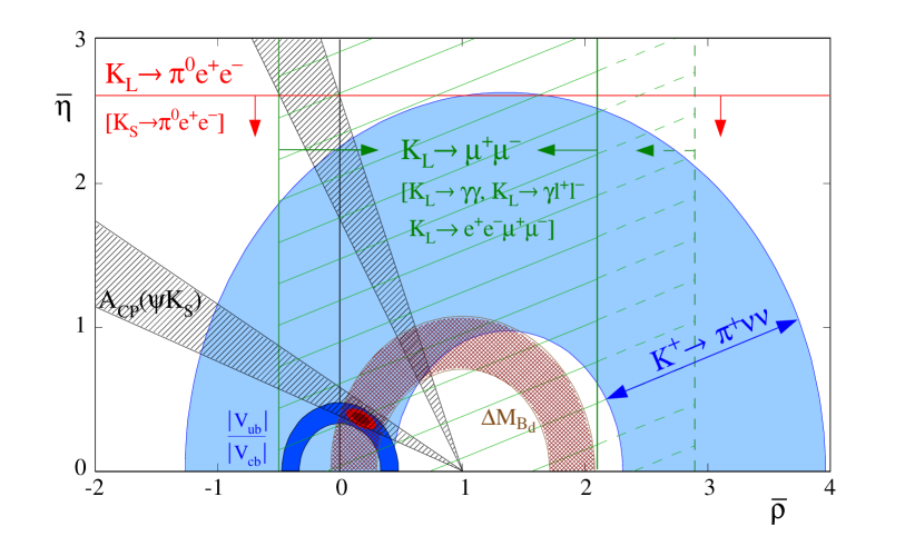
Figure 4: Summary of the present constraints in the $\bar{\rho}$–$\bar{\eta}$ plane from rare $K$ decays: the $K_{L}\to\mu^{+}\mu^{-}$ bound on $\bar{\rho}$ discussed in this work (with and without the sign estimate); the $K_{L}\to\pi^{0}e^{+}e^{-}$ bound on $\bar{\eta}$ [26] and the $K^{+}\to\pi^{+}\nu\bar{\nu}$ ellipse [27]. The constraints on $|V_{ub}|$ and $B$–$\bar{B}$ mixing, from Ref. [15], are also shown for comparison.

As can be seen in Fig. 4, this bound does not compete in precision with present CKM constraints from $B$ physics; however, it does compete with constraints from other $\Delta S=1$ FCNC processes, such as $K^{+}\to\pi^{+}\nu\bar{\nu}$. The interest of these bounds is their implications for non-standard scenarios. For instance, using Eq. (12), the $K_{L}\to\mu^{+}\mu^{-}$ bound leads to

$$-2.2\ (-3.3)<\frac{{\rm Re}\left(Z_{ds}\right)}{{\rm Re}\left(Z_{ds}^{\rm SM}\right)}<2.2~{},$$ (35)

which is one of the most stringent constraints on possible non-standard FCNC couplings of the $Z$ boson.

5 $K_{S}\to\mu^{+}\mu^{-}$

The most general decomposition of $K^{0}~{}(\bar{K}^{0})\to\ell^{+}\ell^{-}$ decay amplitudes does not include only the $s$-wave ($A$) component in Eq. (1), but also a $p$-wave ($B$) term:

$${\cal A}(K^{0}\to\ell^{+}\ell^{-})=\bar{u}_{\ell}(iB+A\gamma_{5})v_{\ell}~{},$$ (36)

with a corresponding decay rate given by [28]

$$\Gamma(K_{L,S}\to\ell^{+}\ell^{-})=\frac{m_{K}\beta_{\ell}}{8\pi}\left(|A|^{2}+\beta_{\ell}^{2}|B|^{2}\right)~{},\qquad\beta_{\ell}=\left(1-\frac{4m_{\ell}^{2}}{m_{K}^{2}}\right)^{1/2}~{}.$$ (37)

The two amplitudes have opposite CP, such that CP-conserving contributions to $K_{L}$ and $K_{S}$ decays are generated by $A$ and $B$, respectively. Long-distance contributions generated by intermediate two-photon states can lead to both $A$ and $B$ amplitudes, but in both cases these have a negligible CP-violating component. Short-distance contributions of the SM type can contribute only to the $A$ amplitude, but in this case CP-violating phases are expected to be ${\cal O}(1)$. For this reason, within the SM and in any SM extension with the same basis of effective FCNC operators, we can safely neglect the $B$ term in the $K_{L}\to\mu^{+}\mu^{-}$ amplitude (as we have done so far). On the other hand, in the $K_{S}\to\mu^{+}\mu^{-}$ case we need to keep both types of amplitudes and we can write

$$\Gamma(K_{S}\to\ell^{+}\ell^{-})=\frac{m_{K}\beta_{\ell}}{8\pi}\left[({\rm Im}A_{\rm short})^{2}+\beta_{\ell}^{2}({\rm Re}B_{\gamma\gamma})^{2}+\beta_{\ell}^{2}({\rm Im}B_{\gamma\gamma})^{2}\right]~{}.$$ (38)

The remarkable feature of Eq. (1) is the fact that the three contributions add incoherently in the total rate. It is then much simpler to derive constraints on the short-distance component from the experimental limit on $\Gamma(K_{S}\to\ell^{+}\ell^{-})$: in the most conservative case, we can derive a model-independent bound on $|{\rm Im}A_{\rm short}|$ simply setting to zero the long-distance terms.

Analogously to Eq. (9), within the SM one finds

$${\rm Im}A_{\rm short}^{\rm SM}=-\frac{G_{F}\alpha_{\rm em}(M_{Z})}{\pi\sin^{2}\theta_{W}}\sqrt{2}m_{\mu}F_{K}{\rm Im}(V_{ts}^{*}V_{td})Y(x_{t})$$ (39)

which leads to

$$B(K_{S}\to\mu^{+}\mu^{-})^{\rm SM}_{\rm short} = 1.0\times 10^{-5}\times\left|{\rm Im}(V_{ts}^{*}V_{td})\right|^{2}$$ (40)

$$= 1.4\times 10^{-12}\times\left|\frac{V_{cb}}{0.041}\right|^{4}\times\left|\frac{\lambda}{0.223}\right|^{2}\times\bar{\eta}^{2}~{}.$$

According to the value of $\bar{\eta}$ obtained from global CKM fits, this contribution is in the $10^{-13}$ range. However, the present constraints on $\bar{\eta}$ derived only from $\Delta S=1$ FCNC processes are rather weak (see Fig. 4): this implies that, at present, new-physics scenarios where $B(K_{S}\to\mu^{+}\mu^{-})_{\rm short}$ reaches the $10^{-11}$ level are perfectly allowed.

Contrary to the $K_{L}\to\mu^{+}\mu^{-}$ case, the dispersive long-distance $K_{S}\to\mu^{+}\mu^{-}$ amplitude is unambiguously determined at the lowest order in the chiral expansion: it arises by two-loop diagrams of the type $K_{S}\to\pi^{+}\pi^{-}\to\gamma\gamma\to\mu^{+}\mu^{-}$, which are finite due to the absence of corresponding local terms [12]. The dispersive amplitude is about 2.3 times the absorptive one, and summing the two contributions Ecker and Pich found [12]:

$$B(K_{S}\to\mu^{+}\mu^{-})_{\rm\gamma\gamma}=1.9\times 10^{-6}\times B(K_{S}\to\gamma\gamma)\approx 5\times 10^{-12}~{}.$$ (41)

Due to possible higher-order chiral corrections, this prediction is expected to hold within a $30\%$ error.

Comparing Eq. (40) and Eq. (41), we conclude that a search for $K_{S}\to\mu^{+}\mu^{-}$ in the $10^{-11}$ range would be very useful. An evidence of $K_{S}\to\mu^{+}\mu^{-}$ well above $10^{-11}$ would be a clear signal of new physics. In absence of a signal, as expected within the SM, bounds on $B(K_{S}\to\mu^{+}\mu^{-})$ close to $10^{-11}$ could be translated into interesting model-independent bounds on the CP-violating phase of the $s\to d\ell^{+}\ell^{-}$ amplitude.

6 Conclusions

The short-distance dominated $\Delta S=1$ FCNC transitions are a key element to investigate the mechanism of quark-flavor mixing, and the rare decays $K_{L,S}\to\mu^{+}\mu^{-}$ represent one of the most useful experimental probes of these processes. In this paper we have re-analyzed the extraction of short-distance constraints from $K_{L}\to\mu^{+}\mu^{-}$. To this purpose, we have quantified the uncertainty of the long-distance $K_{L}\to\gamma\gamma\to\mu^{+}\mu^{-}$ amplitude. The latter has been evaluated employing a semi-phenomenological approach to the $K_{L}\to\gamma\gamma$ form factor. At short-distances, this approach is essentially equivalent to the one of Ref. [8, 9]; however, the semi-phenomenological approach is superior in the low-energy region, where it takes into account the precise experimental constraints on the Dalitz modes. As we have shown, this region provides the dominant contribution to the dispersive integral needed to evaluate the $K_{L}\to\gamma\gamma\to\mu^{+}\mu^{-}$ amplitude.

The short-distance bounds thus derived, expressed as effective bounds on the CKM parameter $\bar{\rho}$, are summarized in Fig. 4. Although not competitive with $B$-physics constraints, these bounds provide a serious challenge to many NP models. The present range is mainly determined by the theoretical error of the approach and it will be very hard to decrease it by means of experimental data only. A minor improvement could be expected with better data on the ratio $\Gamma(K_{L}\to\mu^{+}\mu^{-})/\Gamma(K_{L}\to\pi^{+}\pi^{-})$ and thus a smaller error in Eq. (8). As we have stressed, a major improvement could be obtained by means of Lattice-QCD calculations of the $K_{L}\to\gamma\gamma$ form factor in the Euclidean region.

Finally, we have briefly discussed the possibility to extract short-distance constrains also from $K_{S}\to\mu^{+}\mu^{-}$. As we have shown, bounds on $B(K_{S}\to\mu^{+}\mu^{-})$ close to $10^{-11}$ could be translated into interesting model-independent bounds on the CP-violating phase of the $s\to d\ell^{+}\ell^{-}$ amplitude.

References

• [1] G. D’Ambrosio, G. Isidori and J. Portoles, Phys. Lett. B 423 (1998) 385 [hep-ph/9708326].
• [2] D. Ambrose et al. [E871 Collaboration], Phys. Rev. Lett. 84 (2000) 1389.
• [3] A. Alavi-Harati et al. [KTeV Collaboration], Phys. Rev. Lett. 87 (2001) 071801.
• [4] A. Alavi-Harati et al. [KTeV Collaboration], Phys. Rev. Lett. 90 (2003) 141801 [hep-ex/0212002].
• [5] M. Corcoran, talk presented at Workshop on $\,e^{+}e^{-}$ in the 1-2 GeV range (Alghero, 10-13 September 2003, http://www.lnf.infn.it/conference/d2/)
• [6] A. Lai et al. [NA48 Collaboration], Phys. Lett. B 551 (2003) 7 [hep-ex/0210053].
• [7] M. Adinolfi et al. [KLOE Collaboration], Phys. Lett. B 566 (2003) 61 [hep-ex/0305035].
• [8] M. Knecht, S. Peris, M. Perrottet and E. de Rafael, Phys. Rev. Lett. 83 (1999) 5230 [hep-ph/9908283].
• [9] D. Greynat and E. de Rafael, hep-ph/0303096.
• [10] D. Gomez Dumm and A. Pich, Phys. Rev. Lett. 80 (1998) 4633 [hep-ph/9801298].
• [11] G. Valencia, Nucl. Phys. B 517 (1998) 339 [hep-ph/9711377].
• [12] G. Ecker and A. Pich, Nucl. Phys. B 366 (1991) 189.
• [13] B.R. Martin, E. de Rafael and J. Smith, Phys. Rev. D 2 (1970) 179.
• [14] G. Buchalla, A.J. Buras and M.E. Lautenbacher, Rev. Mod. Phys. 68 (1996) 1125 [hep-ph/9512380].
• [15] M. Battaglia et al., hep-ph/0304132.
• [16] L. Littenberg, hep-ex/0212005.
• [17] K. Hagiwara et al., Phys. Rev. D 66 (2002) 010001 and 2003 off-year partial update for the 2004 edition available on the PDG WWW pages (URL: http://pdg.lbl.gov/).
• [18] Y. Nir and D. Silverman, Phys. Rev. D 42 (1990) 1477;
G. Colangelo and G. Isidori, JHEP 09 (1998) 009.
• [19] A.J. Buras and L. Silvestrini, Nucl. Phys. B 546 (1999) 299.
• [20] A. J. Buras, R. Fleischer, S. Recksiegel and F. Schwab, hep-ph/0309012;
D. Atwood and G. Hiller, hep-ph/0307251.
• [21] C. Quigg and J.D. Jackson, preprint UCRL 18487 (1968), unpublished;
M.B. Voloshin and E.P. Shabalin, JETP Lett. 23 (1976) 107;
R.E. Shrock and M.B. Voloshin, Phys. Lett. B 87 (1980) 375;
L. Bergström, E. Massó and P. Singer, Phys. Lett. B 131 (1983) 229; Phys. Lett. B 249 (1990) 141.
• [22] M. Knecht, S. Peris and E. de Rafael, Phys. Lett. B 443 (1998) 255 [hep-ph/9809594].
• [23] A. R. Barker, H. Huang, P. A. Toale and J. Engle, Phys. Rev. D 67 (2003) 033008 [hep-ph/0210174].
• [24] M. Beneke, G. Buchalla, M. Neubert and C. T. Sachrajda, Phys. Rev. Lett. 83 (1999) 1914 [hep-ph/9905312]; M. Beneke, G. Buchalla, M. Neubert and C. T. Sachrajda, Nucl. Phys. B 591 (2000) 313 [hep-ph/0006124].
• [25] A. Pich and E. de Rafael, Phys. Lett. B 374 (1996) 186 [hep-ph/9511465].
• [26] G. Buchalla, G. D’Ambrosio and G. Isidori, Nucl. Phys. B 672 (2003) 387 [hep-ph/0308008].
• [27] S. Adler et al. [E787 Collab.], Phys. Rev. Lett. 88 (2002) 041803 [hep-ex/0111091]; G. Isidori, hep-ph/0307014.
• [28] G. D’Ambrosio, G. Ecker, G. Isidori and H. Neufeld, in The Second DA$\Phi$NE Physics Handbook, Eds. L. Maiani, G. Pancheri and N. Paver, (SIS Frascati, 1995), hep-ph/9411439.