Towards understanding $b\overline{b}$ production in $\gamma\gamma$ collisions

Jiří Chýla

Abstract

The data on the total cross section $\sigma_{tot}($e⁺e${}^{-}\rightarrow$e⁺e${}^{-}b\overline{b})$ measured at LEP2 represent a serious challenge for perturbative QCD. In order to understand the origin of the discrepancy between the data and QCD calculations, we investigate the dependence of four contributions to this cross section on $\gamma\gamma$ collision energy. As the reliability of the existing calculations of $\sigma_{tot}($e⁺e${}^{-}\rightarrow$e⁺e${}^{-}b\overline{b})$ depends, among other things, on the stability of the calculations of the cross section $\sigma_{tot}(\gamma\gamma\rightarrow b\overline{b})$ with respect to variations of the renormalization and factorization scales, we investigate this aspect in detail. We show that in most of the region relevant for the LEP2 data the existing QCD calculations of the cross section $\sigma_{tot}(\gamma\gamma\rightarrow b\overline{b})$ do not exhibit a region of local stability. Possible source of this instability is suggested and its phenomenological implications for understanding the LEP2 data are discussed.

1 Introduction

Heavy quark production in hard collisions of hadrons, leptons and photons has been considered as a clean test of perturbative QCD. It has therefore come as a surprise that the first data on the $\overline{b}b$ production in $\overline{\mathrm{p}}$p collisions at the Tevatron [1, 2], $\gamma$p collisions at HERA [3, 4] and $\gamma\gamma$ collisions at LEP2 [5, 6] have turned out to lie significantly and systematically above theoretical calculations. The disagreement between data [5, 6] and theory [7, 8, 9] was particularly puzzling for the collisions of two quasireal photons at LEP2.

The arrival of new data on $\overline{b}b$ production in ep collisions at HERA [10], shown in the left part of Fig. 1 as solid squares, have further complicated the situation. In the range of moderate $Q^{2}\simeq 80$ GeV² the new ZEUS data [10] are in reasonable agreement with NLO QCD predictions and also in the photoproduction region the excess of the new data over theory is substantially smaller then that in the older data. As a result, there is now an inconsistency between new ZEUS and older H1 results [3] for moderate $Q^{2}$, but the situation remains unclear also in the photoproduction region. For $\overline{\mathrm{p}}$p collisions the progress on the theoretical side [11, 12] has significantly reduced the discrepancy observed at the Tevatron.

On the other hand, the problem of understanding the $\overline{b}b$ production in $\gamma\gamma$ collisions remains. The preliminary DELPHI data presented this spring at PHOTON 2003 conference [13] and reproduced in Fig. 1, are in striking agreement with the older L3 and OPAL data. The central values of all three experiments are almost identical which strongly supports the reliability of these measurements.

Figure 1: The current situation with data on $\overline{b}b$ production in ep and e⁺e^- collisions, including the most recent data of ZEUS [10] and DELPHI [13].

Contrary to the case of analogous discrepancy in antiproton-proton collisions at the Tevatron, there have been few theoretical suggestions how to explain the sizable excess of data over current theory in $\gamma\gamma$ collisions. Neither the use of unintegrated parton distribution functions [14], nor the production of supersymmetric particles [15], proposed for explaining an analogous excess in antiproton-proton collisions, are of much help for LEP2 data, primarily because of low $\gamma\gamma$ energies involved. Quite recently, however, this discrepancy has been interpreted as an evidence for integer quark charges [16]. We will come back to this suggestion in Section 4.1.

In [12] we have investigated the sensitivity of QCD calculations of $\sigma_{tot}(p\overline{p}\rightarrow b\overline{b};S,M,\mu)$ to the variation of the renormalization and factorization scales $\mu$ and $M$. In particular we have argued that in order to arrive at locally stable results [17] these two scales must be kept independent. We have furthermore shown that in the Tevatron energy range the position of the saddle point of the cross section $\sigma_{tot}(p\overline{p}\rightarrow b\overline{b};S,M,\mu)$ lies far away from the “diagonal” $\mu=M$ used in all existing calculations. Using the NLO prediction at the saddle point instead of the conventional choice $\mu=M=m_{b}$ enhances the theoretical prediction in the Tevatron energy range by a factor of about 2, which may help explaining the excess of data over NLO QCD predictions.

In this paper similar analysis is performed for $\gamma\gamma$ collisions at the total centre of mass energies $W$ relevant for existing LEP2 data. The specific features of the theoretical description of $Q\overline{Q}$ production in $\gamma\gamma$ collisions have been discussed in [18]. However, as all three experiments at LEP2 have measured merely an integral over the cross section $\sigma(\gamma\gamma\rightarrow b\overline{b},W)$ weighted by the product of photon fluxes inside the beam electrons and positrons, it is important to understand the $W$-dependence of the four individual contributions to it.

The paper is organized as follows. The basic facts and formulae relevant for the quantitative investigation of renormalization and factorization scale dependence of finite order QCD approximations are collected in Section 2. This is followed in Section 3 by the discussion of the general form of $\sigma_{tot}(\gamma\gamma\rightarrow b\overline{b};W,M,\mu)$. In Section 4 the $W$-dependence of the four contributions to the cross section $\sigma_{tot}($e⁺e${}^{-}\rightarrow$e⁺e${}^{-}b\overline{b})$ is investigated at the LO of QCD. The quantitative role of NLO corrections and the implications of the (in)stability of existing calculations of $\sigma_{tot}^{\mathrm{NLO}}(\gamma\gamma\rightarrow b\overline{b})$ for explaining the observed puzzle is discussed in Section 5. The conclusions are drawn in Section 6.

2 Basic facts and formulae

The basic quantity of perturbative QCD calculations, the renormalized color coupling $\alpha_{s}(\mu)$, depends on the renormalization scale $\mu$ in a way governed by the equation

$$\frac{{\mathrm{d}}\alpha_{s}(\mu)}{{\mathrm{d}}\ln\mu^{2}}\equiv\beta(\alpha_{s}(\mu))=-\frac{\beta_{0}}{4\pi}\alpha_{s}^{2}(\mu)-\frac{\beta_{1}}{16\pi^{2}}\alpha_{s}^{3}(\mu)+\cdots,$$ (1)

where for $n_{f}$ massless quarks $\beta_{0}=11-2n_{f}/3$ and $\beta_{1}=102-38n_{f}/3$. Its solutions depend beside $\mu$ also on the renormalization scheme (RS). At the NLO this RS can be specified via the parameter $\Lambda_{\mathrm{RS}}$ corresponding to the renormalization scale for which $\alpha_{s}$ diverges. The coupling $\alpha_{s}(\mu)$ then solves the equation

$$\frac{\beta_{0}}{4\pi}\ln\left(\frac{\mu^{2}}{\Lambda^{2}_{\mathrm{RS}}}\right)=\frac{1}{\alpha_{s}(\mu)}+c\ln\frac{c\alpha_{s}(\mu)}{1+c\alpha_{s}(\mu)},~{}~{}c\equiv\beta_{1}/(4\pi\beta_{0}).$$ (2)

At the NLO the coupling $\alpha_{s}$ is a function of the ratio $\mu/\Lambda_{\mathrm{RS}}$ and the variation of the RS for fixed scale $\mu$ is therefore equivalent to the variation of $\mu$ for fixed RS. To vary both the renormalization scale and scheme is legitimate, but redundant. Throughout the paper I will work in the conventional $\overline{\mathrm{MS}}$ RS and vary the renormalization scale $\mu$ only. As we shall investigate the QCD predictions down to quite small values of the renormalization scale $\mu$, the equation (2) will be solved numerically, rather than expanding its solution in inverse powers of $\ln(\mu/\Lambda)$.

The main difference between hard collisions of hadrons and photons comes from the fact that quark and gluon distribution functions of the photon

$$\Sigma(x,M)\equiv\sum_{i=1}^{n_{f}}\left(q_{i}(x,M)+\overline{q}_{i}(x,M)\right),~{}q_{\mathrm{NS}}(x,M)\equiv\sum_{i=1}^{n_{f}}\left(e_{i}^{2}-\langle e^{2}\rangle\right)\left(q_{i}(x,M)+\overline{q}_{i}(x,M)\right)$$ (3)

satisfy the system of coupled inhomogeneous evolution equations

$$\frac{{\mathrm{d}}\Sigma(M)}{{\mathrm{d}}\ln M^{2}} = \delta_{\Sigma}k_{q}(M)+P_{qq}(M)\otimes\Sigma(M)+P_{qG}(M)\otimes G(M),$$ (4)

$$\frac{{\mathrm{d}}G(M)}{{\mathrm{d}}\ln M^{2}} = k_{G}(M)+P_{Gq}(M)\otimes\Sigma(M)+P_{GG}(M)\otimes G(M),$$ (5)

$$\frac{{\mathrm{d}}q_{\mathrm{NS}}(M)}{{\mathrm{d}}\ln M^{2}} = \delta_{\mathrm{NS}}k_{q}(M)+P_{\mathrm{NS}}(M)\otimes q_{\mathrm{NS}}(M),$$ (6)

where $\delta_{\mathrm{NS}}\equiv 6n_{f}\left(\langle e^{4}\rangle-\langle e^{2}\rangle^{2}\right)$, $\delta_{\Sigma}=6n_{f}\langle e^{2}\rangle$ and

$$k_{q}(x,M) = \frac{\alpha}{2\pi}\left[k^{(0)}_{q}(x)+\frac{\alpha_{s}(M)}{2\pi}k_{q}^{(1)}(x)+\left(\frac{\alpha_{s}(M)}{2\pi}\right)^{2}k^{(2)}_{q}(x)+\cdots\right],$$ (7)

$$k_{G}(x,M) = \frac{\alpha}{2\pi}\left[~{}~{}~{}~{}~{}~{}~{}~{}~{}~{}~{}~{}\frac{\alpha_{s}(M)}{2\pi}k_{G}^{(1)}(x)+\left(\frac{\alpha_{s}(M)}{2\pi}\right)^{2}k^{(2)}_{G}(x)+\cdots\;\right],$$ (8)

$$P_{ij}(x,M) = ~{}~{}~{}~{}~{}~{}~{}~{}~{}~{}~{}~{}~{}~{}~{}~{}~{}~{}\frac{\alpha_{s}(M)}{2\pi}P^{(0)}_{ij}(x)+\left(\frac{\alpha_{s}(M)}{2\pi}\right)^{2}P_{ij}^{(1)}(x)+\cdots.$$ (9)

The lowest order inhomogeneous splitting function $k_{q}^{(0)}(x)=(x^{2}+(1-x)^{2})$ as well as the homogeneous splitting functions $P^{(0)}_{ij}(x)$ are unique, whereas all higher order splitting functions $k^{(j)}_{q},k^{(j)}_{G},P^{(j)}_{kl},j\geq 1$ depend on the choice of the factorization scheme (FS). Although potentially important, I will not exploit this freedom and throughout this paper will stay within the $\overline{\mathrm{MS}}$ FS. The equations (4-6) can be recast into evolution equations for $q_{i}(x,M),\overline{q}_{i}(x,M)$ and $G(x,M)$ with inhomogeneous splitting functions $k_{q_{i}}^{(0)}=3e_{i}^{2}k_{q}^{(0)}$.

Due to the presence of the inhomogeneous terms on the r.h.s. of (4-6) their general solutions can be written as a sum of a particular solution of the full inhomogeneous equations and a general solution, called hadron-like (HAD), of the corresponding homogeneous ones. A subset of the former resulting from the resummation of contributions of diagrams in Fig. 2 describing multiple parton emissions off the primary QED vertex $\gamma\rightarrow q\overline{q}$ and vanishing at $M=M_{0}$, are called point-like (PL) solutions.

Figure 2: Diagrams defining the pointlike parts of the nonsinglet quark and gluon distribution functions of the photon, represented by the symbols on the left.

Due to the arbitrariness in the choice of $M_{0}$ the separation

$$D(x,M)=D^{\mathrm{PL}}(x,M,M_{0})+D^{\mathrm{HAD}}(x,M,M_{0}).$$ (10)

is, however, ambiguous. The explicit form of the pointlike contribution to nonsinglet distribution function

$$q_{\mathrm{NS}}^{\mathrm{PL}}(n,M_{0},M)=\frac{4\pi}{\alpha_{s}(M)}\left[1-\left(\frac{\alpha_{s}(M)}{\alpha_{s}(M_{0})}\right)^{1-2P^{(0)}_{qq}(n)/\beta_{0}}\right]a_{\mathrm{NS}}(n),~{}~{}a_{\mathrm{NS}}(n)\equiv\frac{\alpha}{2\pi\beta_{0}}\frac{k_{\mathrm{NS}}^{(0)}(n)}{1-2P^{(0)}_{qq}(n)/\beta_{0}}$$ (11)

is often claimed to imply that it behaves as ${\cal O}(\alpha/\alpha_{s})$. However, the fact that $\alpha_{s}(M)$ appears in the denominator of $q^{\mathrm{PL}}_{\mathrm{NS}}$ cannot be interpreted in this way [19] because switching QCD off by sending $\Lambda_{\mathrm{RS}}\rightarrow 0$ for fixed $M,M_{0}$ reduces, as expected, the expression (11) to the purely QED contribution, corresponding to the first diagram in in the upper part of Fig. 2

$${q^{\mathrm{PL}}_{\mathrm{NS}}(x,M,M_{0})\rightarrow}{\frac{\alpha}{2\pi}k_{\mathrm{NS}}^{(0)}(x)\ln\frac{M^{2}}{M_{0}^{2}}}.$$ (12)

The form (11) merely implies that for asymptotically large $M$ the pointlike part $q^{\mathrm{PL}}_{\mathrm{NS}}$ is proportional to $\ln M$.

As emphasized long time ago by Politzer [20] there is no compelling reason for identifying the renormalization and factorization scales $\mu$ and $M$ and one should therefore keep these scale as independent free parameters of any finite order perturbative calculations.

3 $Q\overline{Q}$ production in $\gamma\gamma$ collisions

We shall first recall the general form of the perturbative expansion of the cross section $\sigma_{tot}(\gamma\gamma\rightarrow Q\overline{Q};W)$ and then discuss in detail the renormalization and factorization scale dependence of finite order approximations to the three QCD contributions to this cross section.

3.1 General form of $\sigma_{tot}(\gamma\gamma\rightarrow Q\overline{Q})$

In the calculations of refs. [7, 8, 9], performed with fixed pole quark masses, the NLO QCD approximation to $\sigma_{tot}(\gamma\gamma\rightarrow Q\overline{Q})$ is defined by taking into account the first two terms in the expansions of direct, as well as single and double resolved photon contributions. Up to the order $\alpha_{s}^{3}$ and suppressing the dependence on $\gamma\gamma$ collision energy $W$ these expansions read

$$\sigma_{\mathrm{dir}}(M) = \sigma_{\mathrm{dir}}^{(0)}+\sigma_{\mathrm{dir}}^{(1)}\alpha_{s}(\mu)+\sigma_{\mathrm{dir}}^{(2)}(M,\mu)\alpha_{s}^{2}(\mu)+\sigma_{\mathrm{dir}}^{(3)}(M,\mu)\alpha_{s}^{3}(\mu)+\cdots,~{}$$ (13)

$$\sigma_{\mathrm{sr}}(M) = ~{}~{}~{}\sigma_{\mathrm{sr}}^{(1)}(M)\alpha_{s}(\mu)+\sigma_{\mathrm{sr}}^{(2)}(M,\mu)\alpha_{s}^{2}(\mu)+\sigma_{\mathrm{sr}}^{(3)}(M,\mu)\alpha_{s}^{3}(\mu)+\cdots,$$ (14)

$$\sigma_{\mathrm{dr}}(M) = ~{}~{}~{}~{}~{}~{}~{}~{}~{}~{}~{}~{}~{}~{}~{}~{}~{}~{}~{}~{}~{}~{}~{}~{}~{}~{}~{}\sigma_{\mathrm{dr}}^{(2)}(M)\alpha_{s}^{2}(\mu)+\sigma_{\mathrm{dr}}^{(3)}(M,\mu)\alpha_{s}^{3}(\mu)+\cdots.$$ (15)

Starting at order $\alpha_{s}^{2}$ the direct photon contribution depends also on the factorization scale and therefore mixes with the single and double resolved photon ones. The first two terms in (13) are, however, totally unrelated to any terms in (14) or (15).

The approximations employed in [7, 8, 9] include all terms that are currently known, so we cannot presently do better. On the other hand we should be aware of its theoretical deficiency. The fact that the first two terms of (13-15) start and end at different powers of $\alpha_{s}$ is usually justified by claiming that PDF of the photon, which appear in expressions for $\sigma_{\mathrm{sr}}^{(1,2)}(M)$ and $\sigma_{\mathrm{dr}}^{(2,3)}(M)$, behave as $\alpha/\alpha_{s}$. Consequently, the first terms in all three expressions (13-15) are claimed to be of order $(\alpha_{s})^{0}=1$ and the second ones of order $\alpha_{s}$. However, as emphasized above and argued in detail in [19], the term $\ln M^{2}$ characterizing the large $M$ behaviour of PDF of the photon comes from integration over the transverse degree of freedom of the purely QED vertex $\gamma\rightarrow q\overline{q}$ and cannot therefore be interpreted as $1/\alpha_{s}(M)$.

3.2 Direct photon contribution

For proper treatment of the direct photon contribution (13), the total cross section of e⁺e^- annihilations into hadrons at center-of-mass energy $\sqrt{S}$ provides a suitable guidance. For $n_{f}$ massless quarks we have

$$\sigma_{\mathrm{had}}(\sqrt{S})=\sigma_{\mathrm{had}}^{(0)}(\sqrt{S})+\alpha_{s}(\mu)\sigma_{\mathrm{had}}^{(1)}(\sqrt{S})+\alpha_{s}^{2}(\mu)\sigma_{\mathrm{had}}^{(2)}(\sqrt{S}/\mu)+\cdots=\sigma_{\mathrm{had}}^{(0)}(1+r(\sqrt{S})),$$ (16)

where the term $\sigma_{\mathrm{had}}^{(0)}\equiv(4\pi\alpha^{2}/S)\sum_{f=1}^{n_{f}}e_{f}^{2}$ comes, similarly as $\sigma_{\mathrm{dir}}^{(0)}$ in (13), from pure QED, whereas genuine QCD effects are contained in the quantity

$$r(\sqrt{S})=\frac{\alpha_{s}(\mu)}{\pi}\left[1+\alpha_{s}(\mu)r_{1}(\sqrt{S}/\mu)+\cdots\right].$$ (17)

For the purpose of QCD analysis of the quantity (16) it is a generally accepted practice to discard the lowest order term $\sigma_{\mathrm{had}}^{(0)}$ and denote as the “leading order” the second term in (16), i.e. $\sigma_{\mathrm{had}}^{(0)}\alpha_{s}/\pi$. The adjectives “LO” and “NLO” are thus reserved for genuine QCD effects described by $r(\sqrt{S})$. The rationale for this terminology is simple: to work in a well-defined renormalization scheme of $\alpha_{s}$ requires including in (17) at least first two consecutive powers of $\alpha_{s}(\mu)$. The explicit $\mu$-dependence of $r_{1}(\sqrt{S}/\mu)$ cancels to the order $\alpha_{s}^{2}$ the implicit $\mu$-dependence of the leading order term $\alpha_{s}(\mu)/\pi$ in (17) and thus guarantees that the derivative with respect to $\ln\mu$ of the sum of first two terms in (17) behaves as $\alpha_{s}^{3}$. For purely perturbative quantities like (16) the association of the term “NLO QCD approximation” with a well-defined renormalization scheme is a generally accepted convention, worth retaining for any physical quantity, like the direct photon contribution $\sigma_{\mathrm{dir}}$ in (13).

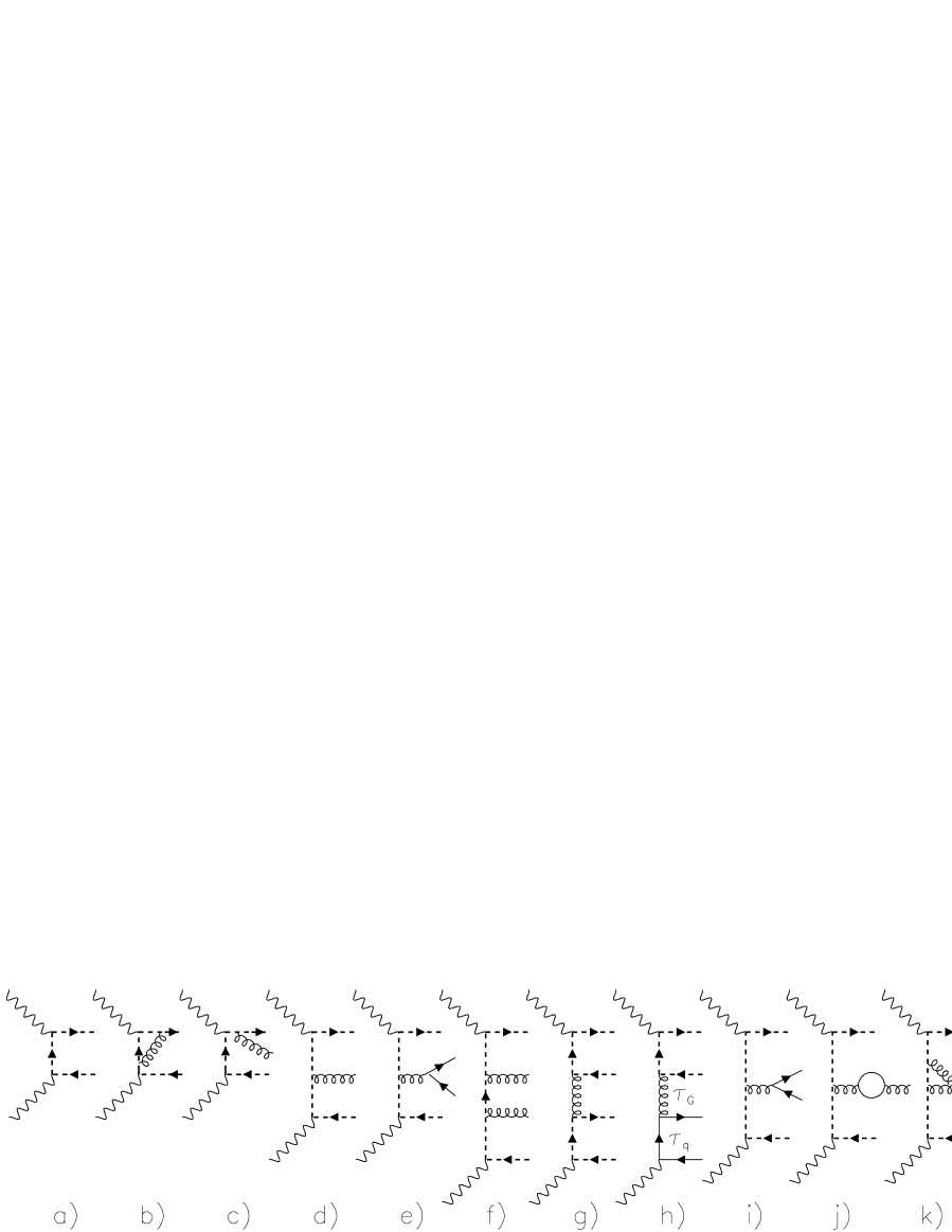
Figure 3: Examples of diagrams describing the direct photon contribution to $\sigma(\gamma\gamma\rightarrow Q\overline{Q})$ up to the order $\alpha^{2}\alpha_{s}^{2}$. The solid (dashed) lines denote light (heavy) quarks.

Contrary to this practice, the calculation in refs. [7, 8, 9] consider the purely QED contribution

$$\sigma^{(0)}_{\mathrm{dir}}(W)=\sigma_{0}\left[\left(1+\frac{4m_{b}^{2}}{W^{2}}-\frac{8m_{b}^{4}}{W^{4}}\right)\ln\frac{1+\beta}{1-\beta}-\beta\left(1+\frac{4m_{b}^{2}}{W^{2}}\right)\right],~{}\sigma_{0}\equiv\frac{12\pi e_{b}^{4}\alpha^{2}}{W^{2}},$$ (18)

where $\beta=\sqrt{1-4m_{b}^{2}/W^{2}}$, as the LO approximation. This is legitimate but implies that their NLO approximation, includes only the lowest order term in $\alpha_{s}$ and cannot therefore be associated to a well-defined renormalization scheme of $\alpha_{s}$. For QCD analysis of $\sigma_{\mathrm{dir}}$ in a well-defined renormalization scheme the incorporation of the third term in (13), proportional to $\alpha^{2}\alpha_{s}^{2}$, is indispensable.

At the order $\alpha^{2}\alpha_{s}^{2}$ the diagrams with light quarks appear and we can distinguish three classes of direct photon contributions, differing by the overall heavy quark charge factor $CF$:

Class A: $CF=e_{Q}^{4}$. Comes from diagrams, like those in Fig. 3e-g, in which both photons couple to heavy $Q\overline{Q}$ pairs. Despite the presence of mass singularities in contributions of individual diagrams coming from gluons and light quarks in the final state and from loops, the KLN theorem implies that at each order of $\alpha_{s}$ the sum of all contributions of this class to $\sigma_{\mathrm{dir}}$ is finite. Note that the first as well as the second terms in (13) are also proportional to $e_{Q}^{4}$ and it is therefore this class of direct photon contributions that is needed for the calculation of $\sigma_{\mathrm{dir}}$ to be performed in a well-defined RS.

Class B: $CF=e_{Q}^{2}$. Comes from diagrams, like that in Fig. 3h, in which one of the photons couples to a heavy $Q\overline{Q}$ and the other to a light $q\overline{q}$ pair. For massless light quarks this diagram has initial state mass singularity, which is removed by introducing the concept of the light quark (and gluon) distribution functions of the photon. The factorization scale dependence of the contribution of this diagram is then related to that of single resolved photon diagrams in Fig. 4a,c.

Class C: $CF=1$. Comes from diagrams in which both photons couple to light $q\overline{q}$ pairs, as those in Fig. 3l. In this case the analogous subtraction procedure relates it to the single resolved photon contribution of the diagram in Fig. 4f and double resolved photon contribution of the diagram in Fig. 4h. The classes B and C are thus needed to guarantee the factorization scale (and scheme) invariance of the single and double resolved photon contributions to order $\alpha^{2}\alpha_{s}^{2}$.

Because of different charge factors $CF$, the classes A, B and C do not mix under renormalization of $\alpha_{s}$ and factorization of mass singularities. As the diagrams in Fig. 3e and 3l give the same final state $q\overline{q}Q\overline{Q}$, we should consider their interference term as well, but it turns out that it does not contribute to the total cross section $\sigma_{tot}(\gamma\gamma\rightarrow Q\overline{Q})$.

3.3 Resolved photon contribution

Figure 4: Examples of resolved photon diagrams involving the pointlike parts of PDF of the photon and the related direct photon diagrams.

The classes B and C of direct photon contributions of the order $\alpha^{2}\alpha_{s}^{2}$ are indispensable to render the sum of direct and resolved photon contributions factorization scale invariant up to order $\alpha^{2}\alpha_{s}^{2}$. To see this in detail, let us write the sum of first two terms in (14-15) explicitly in terms of PDF and parton level cross sections

$$\sigma_{\mathrm{res}}^{(12)}(M,\mu) \!\!\!\equiv\!\!\! 2\alpha_{s}(\mu)\int\!\!{\mathrm{d}}xG(x,M)\left[\sigma_{\gamma G}^{(1)}(x)+\alpha_{s}(\mu)\sigma_{\gamma G}^{(2)}(x,M,\mu)\right]+4\alpha_{s}^{2}(\mu)\int\!\!{\mathrm{d}}x\sum_{i}q_{i}(x,M)\sigma_{\gamma q_{i}}^{(2)}(x,M)+$$ (19)

$$2\alpha_{s}^{2}(\mu)\int\!\!\!\int{\mathrm{d}}x{\mathrm{d}}y\sum_{i}q_{i}(x,M)\overline{q}_{i}(y,M)\left[\sigma_{q\overline{q}}^{(2)}(xy)+\alpha_{s}(\mu)\sigma_{q\overline{q}}^{(3)}(xy,M,\mu)\right]+$$

$$~{}\alpha_{s}^{2}(\mu)\int\!\!\!\int{\mathrm{d}}x{\mathrm{d}}yG(x,M)G(y,M)\left[\sigma_{GG}^{(2)}(xy)+\alpha_{s}(\mu)\sigma_{GG}^{(3)}(xy,M,\mu)\right]+$$

$$2\alpha_{s}^{3}(\mu)\int\!\!\!\int{\mathrm{d}}x{\mathrm{d}}y\Sigma(x,M)G(y,M)\sigma_{qG}^{(3)}(xy,M)$$

where $\sum_{i}q_{i}$ runs over $n_{f}$ quark flavors and the factors of two and four reflect the identity of beam particles and equality of contributions from quarks and antiquarks. Recalling the general form of the derivative

$$\!\!\!\!\!\!\!\frac{{\mathrm{d}}\sigma_{\mathrm{res}}}{{\mathrm{d}}\ln M^{2}}=\int{\mathrm{d}}xW_{0}(x,M)+\!\!\int\!\!{\mathrm{d}}x\!\left[\sum_{i}q_{i}(x,M)W_{q_{i}}(x,M)+G(x,M)W_{G}(x,M)\right]+$$ (20)

$$\!\!\!\!\!\!\!\!\int\!\!\!\!\int\!{\mathrm{d}}x{\mathrm{d}}y\!\left[G(x,M)G(y,M)W_{GG}(xy,M)\!+\!\sum_{i}q_{i}(x,M)\overline{q}_{i}(y,M)W_{q\overline{q}}(xy,M)+\right.$$

$$~{}~{}~{}~{}~{}~{}~{}~{}\Sigma(x,M)G(y,M)W_{qG}(xy,M)\Bigg{]},$$

using (4-6) and denoting $\alpha_{s}\equiv\alpha_{s}(\mu)$, $\dot{f}\equiv\mathrm{d}f/\mathrm{d}\ln M^{2}$ we find

$$W_{0}(x,M) = \frac{\alpha\alpha_{s}^{2}}{\pi}\left\{\frac{1}{2\pi}k_{G}^{(1)}(x)\sigma_{\gamma G}^{(1)}(x)+6k_{q}^{(0)}(x)\sum_{i}e_{i}^{2}\sigma_{\gamma q_{i}}^{(2)}(x,M)\right\}+\cdots$$ (21)

$$W_{q_{i}}(x,M) = \frac{\alpha_{s}^{2}}{\pi}\!\left\{4\pi\dot{\sigma}_{\gamma q}^{(2)}(x)+\!\!\int\!\!{\mathrm{d}}z\!\left[P_{Gq}^{(0)}(z)\sigma_{\gamma G}^{(1)}(xz)+3e_{i}^{2}\alpha k_{q}^{(0)}(z)\sigma_{q\overline{q}}^{(2)}(xz)\right]\right\}\!\!+\cdots$$ (22)

$$W_{G}(x,M) = \frac{\alpha_{s}^{2}}{\pi}\!\left\{2\pi\dot{\sigma}_{\gamma G}^{(2)}(x)+\!\!\int\!\!{\mathrm{d}}zP_{GG}^{(0)}(z)\sigma_{\gamma G}^{(1)}(xz)\right\}+\cdots$$ (23)

$$W_{GG}(x,M) = \frac{\alpha_{s}^{3}}{\pi}\left\{\pi\dot{\sigma}_{GG}^{(3)}(x)+\!\!\int\!\!{\mathrm{d}}zP^{(0)}_{GG}(z)\sigma_{GG}^{(2)}(xz)\right\}+\cdots$$ (24)

$$W_{q\overline{q}}(x,M) = \frac{\alpha_{s}^{3}}{\pi}\left\{2\pi\dot{\sigma}_{q\overline{q}}^{(3)}(x)+2\!\!\int\!\!{\mathrm{d}}zP^{(0)}_{qq}(z)\sigma_{q\overline{q}}^{(2)}(xz)\right\}+\cdots$$ (25)

$$W_{qG}(x,M) = \frac{\alpha_{s}^{3}}{\pi}\left\{2\pi\dot{\sigma}_{qG}^{(3)}(x)+\!\!\int\!\!{\mathrm{d}}z\!\left[P^{(0)}_{qG}(z)\sigma_{q\overline{q}}^{(2)}(xz)+P^{(0)}_{Gq}(z)\sigma_{GG}^{(2)}(xz)\right]\!\right\}\!+\cdots$$ (26)

Only the lowest order terms on the r.h.s. of (21-26) are written out explicitly. All integrals in (22-26) go formally from $0$ to $1$, but threshold behaviour of cross sections $\sigma_{ij}(xz)$ restricts the region to $xz\geq 4m_{Q}^{2}/W^{2}$.

The factorization scale invariance of (19) requires that its variation with respect to $\ln M^{2}$ is of higher order in $\alpha_{s}$ than the approximation itself. There is no dispute that direct photon contributions of classes B and C are needed to guarantee this property. The question is which terms on the r.h.s. of (20) must vanish if the approximation is defined by (19).

In the conventional approach both $q(M)$ and $G(M)$ are claimed to be of order $\alpha/\alpha_{s}$ and the approximation (19) thus of the order $\alpha^{2}\alpha_{s}$, implying that only terms up to this order must vanish in (20). This in turn means that the functions (22-23) must vanish to order $\alpha_{s}^{2}$ and (24-26) to order $\alpha_{s}^{3}$ respectively, which, indeed, they do . The fact that the expression on the r.h.s. of (21) does not vanish is of no concern in this approach as it is manifestly of the order $\alpha\alpha_{s}^{2}$ and thus supposedly of higher order than (19) itself.

If, on the other hand, we take into account that quark and gluon distribution functions of the photon behave as $q(M),G(M)\propto\alpha$, we see that $W_{0}$ is of the same order $\alpha^{2}\alpha_{s}^{2}$ as the products $q_{i}W_{q_{i}},GW_{G}$ and other integrands on the r.h.s. of (20) and must therefore also vanish for theoretical consistency of the approximation (19). This, in turn, necessitates the inclusion of class B direct photon contributions of the order $\alpha\alpha_{s}^{2}$, like those in Fig. 4b,g, which provide the $M$-dependent terms the derivative of which cancels the first term in (20) involving the integral over $W_{0}$. Note that $W_{q_{i}}$ in (22) receives contributions from the derivatives of both single and double resolved photon diagrams, proportional to $\sigma_{\gamma G}$ and $\sigma_{q\overline{q}}$, respectively. This fact reflects the mixing of single and double resolved photon contributions, which starts at the order $\alpha^{2}\alpha_{s}^{2}$ and is due to the presence of the inhomogeneous splitting terms in the evolution equations (4-6). For theoretical consistency of the sum of direct and resolved photon contribution up to the order $\alpha\alpha_{s}^{2}$ only the lowest order double resolved photon contribution must be included.

4 $\overline{b}b$ production at LEP2

We now turn to the phenomenological analysis of $\overline{b}b$ production at LEP2, where the incoming leptons act as sources of transverse and longitudinal virtual photons, described by the fluxes

$$f^{\gamma}_{T}(y,Q^{2}) = \frac{\alpha}{2\pi}\left(\frac{1+(1-y)^{2})}{y}\frac{1}{Q^{2}}-\frac{2m_{\mathrm{e}}^{2}y}{Q^{4}}\right),$$ (27)

$$f^{\gamma}_{L}(y,Q^{2}) = \frac{\alpha}{2\pi}\frac{2(1-y)}{y}\frac{1}{Q^{2}},$$ (28)

where $Q^{2}$ stands for photon virtuality. Although the kinematic region of the LEP data includes photon virtualities up to moderate $Q^{2}$, the cross section of the inclusive process

$${\mathrm{e}}^{+}{\mathrm{e}}^{-}\rightarrow{\mathrm{e}}^{+}{\mathrm{e}}^{-}b\overline{b}+~{}{\mathrm{anything}}$$ (29)

is dominated by the production of the $b\overline{b}$ pair in the collision of two quasireal photons with very small $Q^{2}$, typically $\langle Q^{2}\rangle\simeq 0.01$ GeV². For such small $Q^{2}$ the cross sections of hard processes involving longitudinal virtual photons, which are proportional to $Q^{2}$, are expected to be negligible compared to those of transverse virtual photons. When talking about the production of $b\overline{b}$ in ${\mathrm{e}}^{+}{\mathrm{e}}^{-}$ collisions we shall always mean in association with the ${\mathrm{e}}^{+}{\mathrm{e}}^{-}$ pair, but for brevity of notation shall drop this latter specification, writing $\sigma_{tot}({\mathrm{e}}^{+}{\mathrm{e}}^{-}\rightarrow b\overline{b})$ instead of $\sigma_{tot}({\mathrm{e}}^{+}{\mathrm{e}}^{-}\rightarrow{\mathrm{e}}^{+}{\mathrm{e}}^{-}b\overline{b})$.

Although the data are available only for cross sections integrated over the whole phase space, we shall discuss the contributions ${\mathrm{d}}\sigma_{k}({\mathrm{e}}^{+}{\mathrm{e}}^{-}\rightarrow b\overline{b})/{\mathrm{d}}W$ of individual processes as functions of $\gamma\gamma$ collision energy $W$. The shapes of these contributions can altenatively be characterized by the functions

$$F_{k}(W)\equiv\int_{2m_{b}}^{W}{\mathrm{d}}w\frac{{\mathrm{d}}\sigma_{k}({\mathrm{e}}^{+}{\mathrm{e}}^{-}\rightarrow b\overline{b})}{{\mathrm{d}}w},~{}~{}G_{k}(W)\equiv\int_{W}^{\sqrt{S}}{\mathrm{d}}w\frac{{\mathrm{d}}\sigma_{k}({\mathrm{e}}^{+}{\mathrm{e}}^{-}\rightarrow b\overline{b})}{{\mathrm{d}}w},$$ (30)

which quantify how much of a given contribution is located in the region up to a given $W$ ($F_{k}(W)$) or above it ($G_{k}(W)$). As the available data are not copious enough to measure the differential distribution ${\mathrm{d}}\sigma({\mathrm{e}}^{+}{\mathrm{e}}^{-}\rightarrow b\overline{b})/{\mathrm{d}}W$ the theoretical analysis of the distributions (30) might allow us to invent a strategy how to separate the kinematic region of accessible $W$ into two parts, each dominated by a particular contribution. The relative importance of the individual contributions as a function of $W$ is determined by the ratia

$$r_{k}(W)\equiv\left.\frac{{\mathrm{d}}\sigma_{k}({\mathrm{e}}^{+}{\mathrm{e}}^{-}\rightarrow b\overline{b})}{{\mathrm{d}}W}\right/\frac{{\mathrm{d}}\sigma_{tot}({\mathrm{e}}^{+}{\mathrm{e}}^{-}\rightarrow b\overline{b})}{{\mathrm{d}}W}.$$ (31)

4.1 QED contribution

The pure QED contribution to $\sigma_{tot}({\mathrm{e}}^{+}{\mathrm{e}}^{-}\rightarrow b\overline{b})$ is given as

$$\frac{{\mathrm{d}}\sigma_{\mathrm{QED}}({\mathrm{e}}^{+}{\mathrm{e}}^{-}\rightarrow b\overline{b})}{{\mathrm{d}}W}=\frac{6\alpha^{4}e_{b}^{4}}{\pi S}\frac{A(W)}{W}\left[\left(1+\frac{4m_{b}^{2}}{W^{2}}-\frac{8m_{b}^{4}}{W^{4}}\right)\ln\frac{1+\beta}{1-\beta}-\beta\left(1+\frac{4m_{b}^{2}}{W^{2}}\right)\right],$$ (32)

where

$$A(W)=\!\!\!\int\!\!\!\int\!{\mathrm{d}}y{\mathrm{d}}z\delta\left(\frac{W^{2}}{S}-yz\right)\left[\frac{1+(1-y)^{2}}{y}\right]\left[\frac{1+(1-z)^{2}}{z}\right]\ln\frac{Q^{2}_{max}(1-y)}{m_{e}^{2}y^{2}}\ln\frac{Q^{2}_{max}(1-z)}{m_{e}^{2}z^{2}},$$ (33)

results from convolution of of photon fluxes (27), integrated over the virtualities up to $Q^{2}_{max}$. The convolution (33) can easily be performed analytically and the result inserted into (32). In Fig. 5 we display by the solid curve the result of evaluating (32) for $m_{b}=4.75$ GeV, $\sqrt{S}=200$ GeV and $Q^{2}_{max}=4$ GeV. The distribution vanishes at the threshold $W=2m_{b}$ due to the threshold behaviour of the cross section (18), peaks at about $W=12$ GeV and then drops rapidly off due to the fast decrease of both the photon flux (27) and (18).

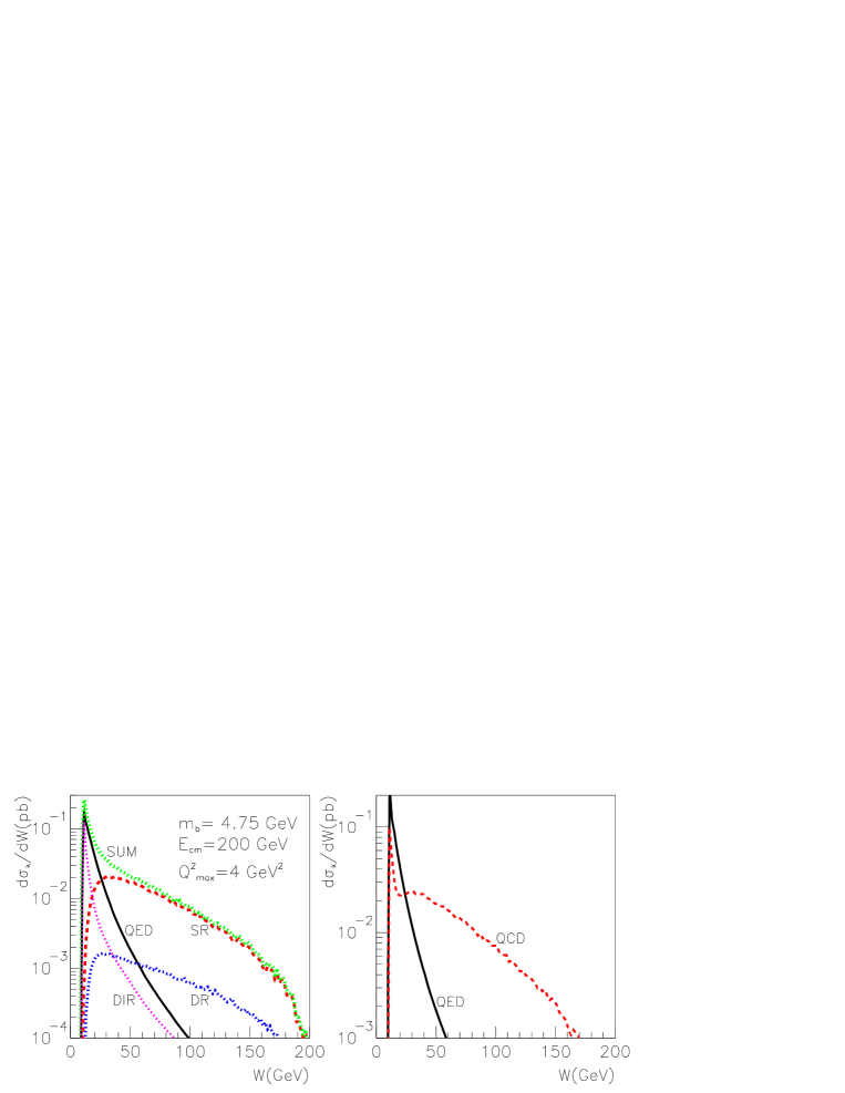
Figure 5: Left: The distributions ${\mathrm{d}}\sigma_{k}/{\mathrm{d}}W$ corresponding to the pure QED contribution together with three lowest order QCD contributions: single resolved (SR), double resolved (DR), and direct (DIR). The sum of all four contributions is shown as the upper dotted curve. Right: the comparison of pure QED contribution with the sum of three lowest order QCD ones. All curves were obtained for $m_{b}=4.75$ GeV, $\sqrt{S}=200$ GeV and $Q^{2}_{max}=4$ GeV² using GRV LO PDF of the photon and setting $\Lambda^{(4)}=0.27$ GeV.

Integrating the distributions in Fig. 5 yields the values in the fourth column of Table 1.

Parameters			QED	LO QCD			Total
$m_{b}$	$\Lambda^{(4)}$	PDF		DIR	SR	DR
$4.75$	$0.27$	GRV LO	1.27	0.473	1.415	0.121	3.28
$4.5$	$0.27$	GRV LO	1.40	0.478	1.746	0.146	3.77
$4.75$	$0.35$	GRV LO	1.27	0.520	1.542	0.141	3.47
$4.75$	$0.27$	SAS1D	1.27	0.473	0.904	0.077	2.73

Table 1: The integrated cross sections $\sigma({\mathrm{e}}^{+}{\mathrm{e}}^{-}\rightarrow b\overline{b},S)$ for $\sqrt{S}=200$ GeV and $Q^{2}_{max}=4$ GeV², corresponding to the distributions in Fig. 5. The renormalization and factorization scales $\mu$ and $M$ we identified and set equal to $m_{b}$. LO form of $\alpha_{s}(\mu)$ was used. All cross sections are in picobarns.

4.2 Leading order QCD corrections

QCD corrections to pure QED expression (18) are of three types: direct (dir), single resolved (sr) and double resolved (dr). We shall first discuss the lowest order contributions to all three types of QCD corrections. As in the case of pure QED contribution, these corrections are given as convolutions of the photon flux (27) with the appropriate partonic cross sections. In all calculations $u,d,s$ and $c$ quarks were considered as intrinsic in the photon and $n_{f}=4$ was taken in the expression for $\alpha_{s}(\mu)$.

4.2.1 Direct photon contribution

The $W$ dependence of the leading order QCD correction is given as the product

$$\frac{{\mathrm{d}}\sigma_{\mathrm{dir}}^{{\mathrm{LO}}}(W)}{{\mathrm{d}}W}=\frac{6\alpha^{4}e_{b}^{4}}{\pi S}\frac{A(W)}{W}\alpha_{s}(\mu)\sigma_{\mathrm{dir}}^{(1)}(W/m_{b})$$ (34)

of the convolution $A(W)$ of photon fluxes and the lowest order QCD contribution $\alpha_{s}(\mu)\sigma_{\mathrm{dir}}^{(1)}(W)$. At this order the direct photon contribution $\sigma_{\mathrm{dir}}^{(1)}\alpha_{s}(\mu)$, which comes form real or virtual emission of one gluon, is exclusively of class A. The function $\sigma_{\mathrm{dir}}^{(1)}(W/m_{b})$ has been calculated in, for instance, [22]. As it is just the first term in the series in positive powers of $\alpha_{s}(\mu)$, the value of the renormalization scale $\mu$ in the argument of $\alpha_{s}(\mu)$ is completely arbitrary. The resulting $W$-dependence, evaluated for $\mu=m_{b}$ and shown in Fig. 5, is peaked even more sharply at small $W$ than the pure QED contribution (32). This reflects the fact that the cross section $\sigma_{\mathrm{dir}}^{(1)}(W/m_{b})$ does not vanish at the threshold $W=2m_{b}$ as does $\sigma_{\mathrm{dir}}^{(0)}(W/m_{b})$.

4.2.2 Resolved photon contribution

The leading-order single and double resolved photon contributions, were computed with HERWIG Monte Carlo event generator, which implements the appropriate LO cross sections of the processes

$$\gamma+G \rightarrow b+\overline{b},$$ (35)

$$G+G \rightarrow b+\overline{b},~{}~{}q+\overline{q}\rightarrow b+\overline{b},$$ (36)

where $q=u,d,s,c$ stand for intrinsic quarks in the photon, and convolutes them with photon fluxes and PDF of the quasireal photon(s). In HERWIG the renormalization and factorization scales $\mu$ and $M$ are identified and set equal to an expression which is approximately equal the transverse mass $\mu=M=M_{T}\equiv\sqrt{E_{T}^{2}+M^{2}}$. In LEP2 energy range the mean $\langle\!M_{T}\!\rangle$ depends weakly on $W$ with, approximately, $\langle\!M_{T}\!\rangle\simeq 7$ GeV.

Results of the calculations in which the LO GRV PDF of the photon, the LO expression for $\alpha_{s}(\mu)$ with $\Lambda^{(4)}=0.27$ GeV and $m_{b}=4.75$ GeV were used, are shown in Fig. 5. As expected, the corresponding distributions are much broader than those of pure QED or LO QCD direct contributions.

4.3 Comparison of individual contributions

The comparison of the distributions ${\mathrm{d}}\sigma_{k}/{\mathrm{d}}W,F_{k}(W)$ and $G_{k}(W)$, corresponding to four individual contributions, displayed in Figs. 5 and 6 and summarized in Table 1, reveals large difference in their shapes and magnitude. Specifically we conclude that

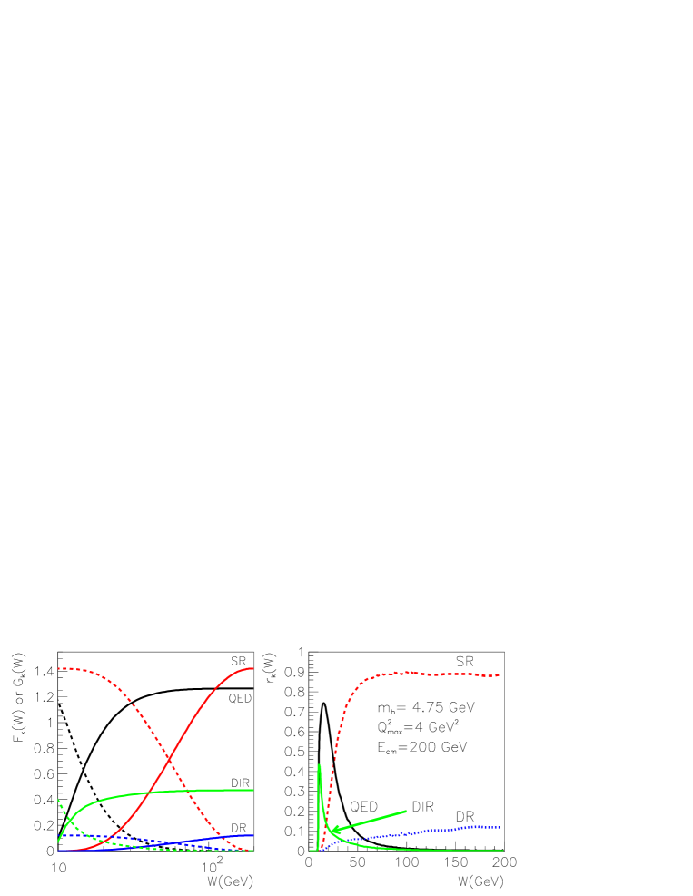
Figure 6: Left: solid (dashed) curves show the partially integrated cross sections $F_{k}(W)$ ($G_{k}(W)$) defined in (30) for QED and three LO QCD contributions. Right: The relative contributions $r_{k}(W)$ defined in (31) for the same four contributions.

• The pure QED as well as the LO direct photon contributions peak at very small $W$ and are basically negligible above $W\simeq 50$ GeV. For instance, the left plot of Fig. 6 shows that $95$% of the QED contribution comes from the region $W\lesssim 30$ GeV.

• The onset of single as well as double resolved photon contributions is much slower, but these distributions are, on the other hand, markedly broader.

• The double resolved photon contribution is negligible everywhere.

• The pure QED and single resolved photon contributions are of comparable size and together make up about 85% of the total integrated cross section,

• up to about $W\simeq 30$ GeV, ${\mathrm{d}}\sigma_{tot}/{\mathrm{d}}W$ is dominated by pure QED contribution, whereas for $W\gtrsim 30$ GeV, QCD contributions take over.

The numbers given in Table 1 correspond to standard colored quarks with fractional electric charges. In [16] the excess of data over standard theoretical calculations is interpreted as evidence for Hahn-Nambu integer quark charges. Applied to the case of b-quark, the author of [16] argues that the correct way of calculating the charge factor in (32) is not the usual $3e^{4}_{b}=1/27$, but $(\sum_{i=1}^{3}e_{b}^{(i)})^{4}/3=1/3=9/27$, where the sum runs over the three Hahn-Nambu integer b-quark charges $e_{b}^{(i)}$, which are $0,0,-1$ respectively. The results is thus $9$ times bigger than that of the standard calculation. I think his argument for first summing over the quark colours and then taking the fourth power is wrong , but I mention it here as illustration of the merit of separating the data into at least two regions of $W$. Were the author of [16] right, the whole discrepancy would have come from the region of small $W$, where QED contribution dominates.

On the other hand, were the light gluino production [15] responsible for the observed excess, the latter would have to come from the region of $W$ dominated by the double resolved photon contribution. Although the energy dependence of the gluon-gluon fusion to gluino-antigluino may be slightly different than those of $G+G\rightarrow Q\overline{Q}$ or $q\overline{q}\rightarrow Q\overline{Q}$, it is clear that the basic shape of the $W$-distribution is given by the convolution of the photon fluxes (27-28) and the gluon distribution function of the photon, which are the same in both types of processes.

The above observations underline the fact that in order to pin down the possible origins of the excess of the integrated cross section $\sigma_{tot}({\mathrm{e}}^{+}{\mathrm{e}}^{-}\rightarrow{\mathrm{e}}^{+}{\mathrm{e}}^{-}b\overline{b})$ over theoretical calculations, it would be very helpful if the data could be separated at least into two subsamples according to their hadronic energy $W$, say $W\lesssim 30$ GeV and $W\gtrsim 30$ GeV.

The magnitude of the contributions discussed in the preceding subsection depend, beside the e⁺e^- cms energy $\sqrt{S}$, on a number of input parameters: the numerical values of $m_{b},\Lambda^{(4)}_{\mathrm{QCD}},Q_{max}^{2}$, the selection of PDF and the choice of the renormalization and factorization scales $\mu$ and $M$. In all the calculation reported above we set $\mu=M=m_{b}$. The central calculation was performed for $\sqrt{S}=200$ GeV, $Q^{2}_{max}=4$ GeV², $m_{b}=4.75$ GeV, $\Lambda^{(4)}=0.27$ GeV using the GRV LO PDF of the photon. To see the sensitivity of the LO results to these assumptions we varied some of these parameters:

• $m_{b}$ was lowered to $m_{b}=4.5$ GeV,

• $\Lambda^{(4)}$ was increased to $0.35$ GeV,

• GRV set of PDF of the photon was replaced with that of Schuler-Sjöstrand set SAS1D.

The choice of $Q^{2}_{max}=4$ GeV² corresponds roughly to the usual cuts imposed on the LEP2 data and could therefore be also adjusted to specific conditions of a given experiment.

The results of the calculations of $\sigma_{tot}({\mathrm{e}}^{+}{\mathrm{e}}^{-}\rightarrow{\mathrm{e}}^{+}{\mathrm{e}}^{-}b\overline{b})$, corresponding to different sets of input parameters specified above, are listed in Table 1. Lowering $m_{b}$ increases all four contributions, as does, except for the pure QED one, increasing $\Lambda^{(4)}$. SAS1D PDF yield markedly lower results for single and double resolved photon contributions. It is, however, clear that varying the input parameters within reasonable bounds does not bring the sum of lowest order QED and QCD calculations significantly closer to the data.

5 Can the NLO QCD corrections solve the puzzle?

With the sum of lowest order QED and QCD contributions to $\sigma_{\mathrm{dir}}^{\mathrm{LO}}({\mathrm{e}}^{+}{\mathrm{e}}^{-}\rightarrow{\mathrm{e}}^{+}{\mathrm{e}}^{-}b\overline{b})$ way below the data we shall now address the question whether the next-to-leading order QCD corrections can at least partly bridge the gap between data a theory.

5.1 Direct photon contribution

The the sum of the second and third terms in (13) can be written, suppressing the dependence of $\sigma_{\mathrm{dir}}^{(i)}$ on the ratio $W/m_{b}$, as

$$\sigma_{\mathrm{dir}}^{\mathrm{NLO}}=\sigma_{\mathrm{dir}}^{(1)}\alpha_{s}(\mu)\left[1+\frac{\sigma_{\mathrm{dir}}^{(2)}(\mu/m_{b})}{\sigma_{\mathrm{dir}}^{(1)}}\alpha_{s}(\mu)\right]=\sigma_{\mathrm{dir}}^{(1)}\alpha_{s}(\mu)\left[1+r_{1}(\mu/m_{b})\alpha_{s}(\mu)\right].$$ (37)

Note that $W^{2}\sigma_{\mathrm{dir}}^{(1)}$ is a unique function of the ratio $W/m_{b}$ and the NLO coefficient $r_{1}(W,m_{b},\mu)$ can be written as a function of $W/m_{b}$ and $m_{b}/\mu$. The first term in (37) is a monotonous function of the renormalization scale $\mu$, spanning the whole interval between zero and infinity. As emphasized in Section 3.2, one needs to include at least the term $\alpha_{s}^{2}\sigma_{\mathrm{dir}}^{(2)}$ to make the expression (37) of genuine next-to-leading order. The class A of order $\alpha^{2}\alpha_{s}^{2}$ direct photon contributions is needed for this purpose.

The renormalization scale invariance of $\sigma_{\mathrm{dir}}^{\mathrm{QCD}}$ implies the following general form of $r_{1}$:

$$r_{1}(W/m_{b},\mu/m_{b},{\mathrm{RS}})=\frac{\beta_{0}}{4\pi}\ln\frac{\mu^{2}}{\Lambda^{2}_{\mathrm{RS}}}-\rho(W/m_{b}),$$ (38)

where $\rho(W/m_{b})$ is a renormalization scale and scheme invariant [17], which, however, depends beside the ratio $W/m_{b}$ also on the numerical value of the ratio $m_{b}/\Lambda^{(4)}$. It can be evaluated using the results of a calculation in any renormalization scheme RS

$$\rho(W/m_{b},m_{b}/\Lambda^{(4)})=\frac{\beta_{0}}{4\pi}\ln\frac{m_{b}^{2}}{\Lambda^{(4)}_{\mathrm{RS}}}-r_{1}(W/m_{b},1,{\mathrm{RS}})$$ (39)

and its numerical value governs basic features of the scale dependence of (37):

Figure 7: a) The renormalization scale dependence of the leading (solid curve) and next-to-leading order contributions to the generic quantity (42) for different values of $\rho$. The dashed curves correspond to $\rho>0$, the dotted ones to $\rho<0$, the dash-dotted to $\rho=0$; b) the same as in a) but plotted in a linear scale of $\mu$; c) graphical representation of (42) in three different renormalazation schemes and for $\rho>0$; d) the shape of the NLO expression (42) as a function of $\alpha_{s}$.

$\rho>0$: the NLO approximation (37) considered as a function of $\mu$ exhibits a local maximum, where ${\mathrm{d}}\sigma_{\mathrm{dir}}^{\mathrm{NLO}}/{\mathrm{d}}\mu=0$ and where the prediction is thus most stable. This point, preferred by the Principle of Minimal Sensitivity [17], is also very close to the point for which $r_{1}=0$, which is selected by method of Effective Charges [21]. The value of $\sigma_{\mathrm{dir}}^{\mathrm{NLO}}$ at this point is proportional to $1/\rho$ implying very large NLO corrections for small $\rho$. Inserting the appropriate numbers for $n_{f}=4$, $m_{b}=4.75$ GeV and $\Lambda^{(4)}_{\overline{\mathrm{MS}}}=0.27$ GeV, we get

$$\rho(W/m_{b})=3.88-r_{1}(W/m_{b},1,\overline{\mathrm{MS}}).$$ (40)

The coefficient $r_{1}(W/m_{b},1,\overline{\mathrm{MS}})$ thus does not have to be large to get small, or even negative $\rho$!

$\rho\leq 0$: $\sigma_{\mathrm{dir}}^{\mathrm{NLO}}$ becomes a monotonous function of $\mu$, similarly to $\sigma_{\mathrm{dir}}^{\mathrm{LO}}$. In fact, taking the derivative of $\sigma_{\mathrm{dir}}^{\mathrm{NLO}}$ with respect to $\mu$ one finds that for $\rho<0$ it is actually even steeper than $\sigma_{\mathrm{dir}}^{\mathrm{LO}}$, given by the first term in (37). Consequently, for negative $\rho$ going to the NLO does not improve the stability of the calculation, but quite on the contrary!

The above features are straightforward to see assuming $\beta_{1}=0$. This assumption simplifies the relevant formulae, but nothing essential depends on it. Setting $c=0$ in (2) allows us to write explicitly

$$\alpha_{s}(\mu)=\frac{4\pi}{\beta_{0}\ln(\mu^{2}/\Lambda^{2}_{\mathrm{RS}})}$$ (41)

which, inserting this expression into (37) and taking into account (38), gives

$$\sigma_{\mathrm{dir}}^{\mathrm{NLO}}=\sigma_{\mathrm{dir}}^{(1)}\alpha_{s}(\mu)\left[2-\rho\alpha_{s}(\mu)\right],$$ (42)

In Fig. 7 we plot the dependence of the generic NLO quantity (42) for several values, positive as well as negative, of $\rho$ and in different renormalization schemes. Several conclusions can be drawn from this figure:

• For $\rho<0$ $\sigma_{\mathrm{dir}}^{\mathrm{NLO}}$ is a steeper function of $\mu$ than $\sigma_{\mathrm{dir}}^{\mathrm{LO}}$. For positive $\rho$, on the other hand, (42) exhibits a local maximum at $\alpha_{s}^{max}=1/\rho$.

• For negative as well as positive values of $\rho$, $\sigma_{\mathrm{dir}}^{\mathrm{NLO}}\propto 1/\ln\mu$ as $\mu\rightarrow\infty$. For negative $\rho$ this implies that there is no region of local stability. However, when plotted on a linear scale of $\mu$ in a limited interval the weak logarithmic does, as illustrated in Fig. 7b, fake the local quasistability.

• The curve representing $\sigma_{\mathrm{dir}}^{\mathrm{NLO}}$ depends, as shown in Fig. 7c for $\rho>0$, on the chosen renormalization scheme. Setting $\mu$ equal to some “natural” physical scale $Q$ therefore does not resolve the renormalization scale ambiguity as in different RS we get different results. However, although also the position of the local maximum depends on the choice of the RS, the value of the NLO approximation (42) at this maximum [17] does not! The same holds for the intersection of the LO and NLO curves [21].

• Instead of varying both the renormalization scale and scheme, which is legitimate but redundant, we may use the couplant $\alpha_{s}$ itself for labeling the different predictions of (42). Instead of an infinite set of curves describing the $\mu$-dependence of $\sigma_{\mathrm{dir}}^{\mathrm{NLO}}(\mu,{\mathrm{RS}})$ in different RS, we get for each $\rho$ a single curve displayed in Fig. 7d.

We wish to emphasize that whereas there are natural physical scales in hard collisions, there is nothing like the “natural” renormalization scheme. The fact that the choice of renormalization scheme is in principle as important as that of the renormalization scale is often not fully appreciated. For instance, the standard way of estimating the importance of higher order corrections beyond the NLO approximation employs the ratio (called “k-factor”) $k\equiv$NLO/LO evaluated for some ”natural” renormalization scale. If this ratio is significantly larger than 1, perturbation theory is deemed unreliable. However, the “k-factors” themselves depend, for a chosen renormalization scale, on the choice of the renormalization scheme and so does therefore also the importance of higher order corrections! The usual procedure of estimating the convergence of a given perturbation expansion by the value of the corresponding “k-factor” evaluated for some ”natural” renormalization scale in the calculationally convenient $\overline{\mathrm{MS}}$ renormalization scheme is thus entirely ad hoc.

As the term $\sigma_{\mathrm{dir}}^{(2)}$ in (37) has not yet been calculated, we cannot associate the class A direct photon contribution, given by the first term in (37), to a well-defined renormalization scheme. Moreover, as the magnitude of the NLO corrections in (37) is determined by the ratio $\sigma_{\mathrm{dir}}^{(2)}(W/m_{b},1)/\sigma_{\mathrm{dir}}^{(1)}(W/m_{b})$ of two functions of $W/m_{b}$, which may depend on $W/m_{b}$ in different ways, the coefficient $r_{1}$ may be very large even when both the numerator and denominator are on average of comparable and small magnitude. The size of NLO correction may also depend sensitively on the ratio $W/m_{b}$. All this indicates that without the knowledge of class A direct photon contribution of the order $\alpha^{2}\alpha_{s}^{2}$, we cannot make a meaningful estimate of the importance of higher order corrections to (37).

5.2 Resolved photon contribution

As in LEP2 energy range the double resolved photon one is numerically negligible, only the single resolved photon contribution will discussed in detail below. As shown in Fig. 5, the spectrum of the contributions ${\mathrm{d}}\sigma_{\mathrm{sr}}/{\mathrm{d}}W$ peaks at about $W=30$ GeV with the mean value $\langle W\rangle\doteq 65$ GeV. The properties of the measured cross section $\sigma_{\mathrm{sr}}^{\mathrm{NLO}}({\mathrm{e}}^{+}{\mathrm{e}}^{-}\rightarrow{\mathrm{e}}^{+}{\mathrm{e}}^{-}b\overline{b})$ will therefore be determined primarily by those of $\sigma_{\mathrm{sr}}^{\mathrm{NLO}}(\gamma\gamma\rightarrow b\overline{b})$ in the energy range $30\lesssim W\lesssim 65$ GeV.

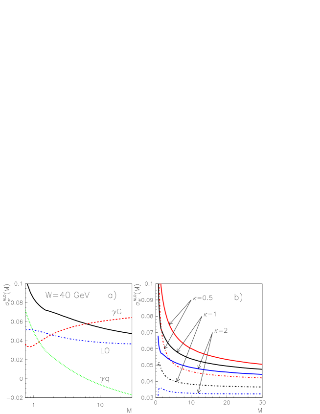
Figure 8: a) The scale dependence of the conventional NLO approximation $\sigma^{\mathrm{NLO}}_{\mathrm{sr}}(W,M,M)$ for $W=40$ GeV (solid curve) together with the contributions of the $\gamma G$ (dashed) and $\gamma q/\overline{q}$ (dotted) channels. The LO approximation is shown for comparison by the dash-dotted curve. b) $\sigma^{\mathrm{NLO}}_{\mathrm{sr}}(W,M,\kappa M)$ (solid curve) and $\sigma^{\mathrm{LO}}_{\mathrm{sr}}(W,M,\kappa M)$ (dash-dotted) for $W=40$ GeV and three values of $\kappa=0.5,1.2$.

All the results shown below for the single resolved photon contribution

$$\sigma^{\mathrm{NLO}}_{\mathrm{sr}}(W,M,\mu) = 2\alpha_{s}(\mu)\int{\mathrm{d}}xG(x,M)\left[\sigma_{\gamma G}^{(1)}(x)+\alpha_{s}(\mu)\sigma_{\gamma G}^{(2)}(x,M,\mu)\right]+$$ (43)

$$4\alpha_{s}^{2}(\mu)\int{\mathrm{d}}x\sum_{i}q_{i}(x,M)\sigma_{\gamma q_{i}}^{(2)}(x,M)$$

are based on the formulae for the partonic cross sections $\sigma^{(k)}_{ij}$ as given in [23]. Even if the reader does not agree with our claim that the approximations employed in [7, 8, 9] do not constitute complete NLO approximation, it is certainly important to understand quantitatively their renormalization and factorization scale dependence. Because the expressions for $\sigma_{\gamma G}^{(2)}$ as given in [23] correspond to $\mu=M$, we have restored its separate dependence on $\mu$ and $M$ by adding to $\sigma_{\mathrm{\gamma G}}^{(2)}(x,M,M)$ the term $(\beta_{0}/4\pi)\sigma_{\gamma G}^{(1)}\ln(\mu^{2}/M^{2})$. Note that for each value of $M$ the expression (43) has, as far as the $\mu$-dependence is concerned, the form of the NLO expression (37). In all calculations the GRV HO set of PDF of the photon and $\Lambda_{\overline{\mathrm{MS}}}^{(4)}=0.27$ GeV were used.

We first follow the conventional procedure and set $M=\mu$. The resulting (common) scale dependence of the expression (43), together with those of the quark and gluon contributions to it, are shown in Fig. 8a for $W=40$ GeV. Overlaid for comparison is also the LO approximation, given by the first term in (43). We note the different scale dependence of the $\gamma G$ and $\gamma q$ channels, the latter turning negative for $M\gtrsim 6$ GeV, but the most important observation concerns the fact that the conventional NLO approximation (43) is a monotonously decreasing function of the scale. Moreover, it falls off even more steeply than the LO expression! In other words in going from the leading to the next-to-leading order the sensitivity to the scale variation increases, rather than decreases, as one might expect (and hope)!

Figure 9: The surface and contour plots of $\sigma^{\mathrm{NLO}}_{\mathrm{sr}}(W,M,\mu)$ for $W=40$ GeV.

Recalling the discussion in Section 5.1 one should, however, not be surprised. To check how much this feature depends on setting exactly $\mu=M$, we plot in Fig. 8b the scale dependence of $\sigma_{\mathrm{sr}}^{\mathrm{NLO}}(W,M,\mu=\kappa M)$ for standard choices of $\kappa=0.5,1,2$. Clearly, the above conclusion is independent of $\kappa$ in this range.

The steep and monotonous scale dependence of $\sigma_{\mathrm{sr}}^{\mathrm{NLO}}(W,M,\mu=\kappa M)$ is a clear warning that the conventional NLO approximation is highly unstable. To see what happens if we relax the usual but arbitrary identification $\mu=\kappa M$ we plot in Fig. 9 the surface and contour plots representing the full $M$ and $\mu$ dependence of $\sigma_{\mathrm{sr}}^{\mathrm{NLO}}(W,M,\mu)$ as given in eq. (43).

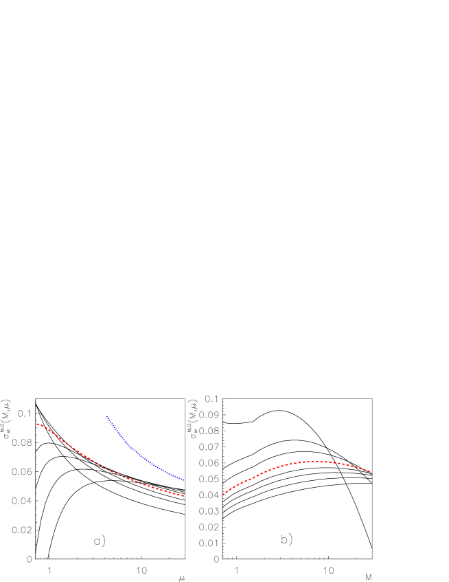
Figure 10: The renormalization scale dependence of $\sigma^{\mathrm{NLO}}_{\mathrm{sr}}(W,M,\mu)$ for fixed values of the factorization scale (a) and vice versa: the factorization scale dependence of $\sigma^{\mathrm{NLO}}_{\mathrm{sr}}(W,M,\mu)$ for the same set of fixed values of the renormalization scale $\mu$ (b). All calculations correspond to $W=40$ GeV. In a) the ordering from above of the curves at $\mu=30$ GeV corresponds to $M=30,16,10,7,4.75,3,2,1$ GeV, in b) the curves correspond at $M=0.7$ GeV to the same sequence from below.

Contrary to analogous process in antiproton-proton collisions [12], it does not exhibit a saddle point, where the derivatives with respect to both $M$ and $\mu$ would vanish, but Fig. 9 seems to indicate some sort of stability region at large scales, say for $M\gtrsim 10$ GeV, $\mu\gtrsim 20$ GeV. This impression is, however, misleading as becomes clear if we plot in Fig. 10 the slices of the surface plot in Fig. 9a along both axis and recall the discussion of Section 5.1. For each fixed value of the factorization scale $M$ the expression (43) has a form of the NLO expression as far as the renormalization scale $\mu$ is concerned. Comparing the curves in Fig. 10a with those of 3a we see that for $M\lesssim 4.2$ GeV $\sigma^{\mathrm{NLO}}_{\mathrm{sr}}(M,\mu)$ corresponds to negative $\rho$ in (42) and thus exhibits no local stability point. For higher $M$ the local maximum in the $\mu$-dependence of $\sigma^{\mathrm{NLO}}_{\mathrm{sr}}(M,\mu)$ exists at the associated $\mu_{max}(M)$. The $M$-dependence of $\sigma^{\mathrm{NLO}}_{\mathrm{sr}}(M,\mu_{max}(M))$, shown in Fig. 10a by the dotted curve, is, however, even steeper that those at fixed $M$. The above plots and conclusions concerned the results at one typical value of $W$, but their essence holds for the whole interval relevant for LEP2 data.

We thus conclude that in the energy range relevant for LEP2 data the renormalization and factorization scale dependence of the conventional NLO calculations of single resolved photon contribution to the total cross section $\sigma_{tot}(\gamma\gamma\rightarrow b\overline{b})$ exhibits no stability region, either as a function of the common scale $\mu=\kappa M$ or as fully two dimensional function of $\mu$ and $M$.

6 Summary and Conclusions

We have argued that in order to understand the origin of the discrepancy between LEP2 data on $b\overline{b}$ production in $\gamma\gamma$ collisions and the current theoretical calculations, two ingredients are needed. On the experimental side, the separation of data into at least two bins of the hadronic energy $W$, say $W\lesssim 30$ GeV and $W\gtrsim 30$ GeV, could be instrumental in pinning down the possible mechanisms or phenomena responsible for the observed excess.

On the theoretical side, the evaluation of the direct photon contribution of the order $\alpha^{2}\alpha_{s}^{2}$ is needed to make the existing theoretical expressions of genuine next-to-leading order in $\alpha_{s}$. In their absence, the existing NLO QCD calculations are highly sensitive to the variation of renormalization and factorization scale and thus inherently unreliable.

References

• [1] B. Abbott et al. (D0 Collab.): Phys. Rev. Lett. 85 (2000), 5068, (hep-ex/0008021)
• [2] D. Acosta et al. (CDF Collab.): Phys. Rev. D65 (2002), 052005, (hep-ex/0111359)
• [3] C. Adloff et al (H1 Collab.): Phys. Lett. B467 (1999), 156, Erratum: Phys. Lett. B518 (2001), 331
• [4] J. Breitweg et al. (ZEUS Collab.): Eur. Phys. J. C18 (2001), 625, (hep-ex/0011081)
• [5] M. Acciarri et al. (L3 Collab.): Phys. Lett. B503 (2001), 10
• [6] OPAL Collab.: OPAL Physics Note PN455, August 2000
• [7] M. Drees, M. KrΓ€mer, J. Zunft, and P. Zerwas, Phys. Lett. B 306 (1993), 371
• [8] M. KrΓ€mer and E. Laenen, Nucl. Phys. B371 (1996), 303
• [9] S. Frixione, M. KrΓ€mer and E. Laenen, Nucl. Phys. B571 (2000), 169
• [10] J. Kroseberg, talk at PHOTON 2003, Frascati, April 2003
• [11] M. Cacciari and P. Nason: Phys. Rev. Lett. 89 (2002), 122003-1
• [12] J. ChΓ½la, JHEP03(2003)042.
• [13] F. Kapusta, talk at PHOTON 2003, Frascati, April 2003
• [14] H. Jung: Phys. Rev. D65 (2002), 034015
• [15] E. Berger et al: Phys. Rev. Lett. 86 (2001), 4231
• [16] P. Ferreira, hep-ph/0309156
• [17] P. M. Stevenson, Phys. Rev. D23 (1981), 2916
• [18] J. ChΓ½la, Proceedings of PHOTON 01, hep-ph/0111469.
• [19] J. ChΓ½la, JHEP04(2000)007.
• [20] H. D. Politzer, Nucl. Phys. B192 (1984), 493
• [21] G. Grunberg, Phys. Rev. D29 (1984), 2315
• [22] J. H. KΓΌhn, E. Mirkes, J. Steegborn, Z. Phys. C 57 (1993), 615
• [23] R. K. Ellis, P. Nason, Nucl. Phys. B312 (1989), 551