A non-perturbative computation of the B-meson decay constant and the b-quark mass in HQET

Abstract

A lattice computation of the B-meson decay constant and the mass of the b-quark to leading order in the heavy quark effective theory is presented. The involved renormalization problems are solved non-perturbatively, and the continuum limit is taken. In the quenched approximation the results reported here already offer an interesting numerical precision, which will be further improved in the near future.

1 Introduction

Not least by the influence of the phenomenologically very interesting programme of current experiments to investigate CP-violation in the B-system BphysExp:2003 , the study of B-meson physics has become a vivid area of research. To interpret the experimental observations within (or beyond) the standard model, matrix elements between low-energy hadron states must be known. But since these QCD matrix elements live in the strongly coupled sector of the theory, they naturally call for a genuinely non-perturbative, ‘ab initio’ approach for their determination: the lattice formulation of QCD, which enables a numerical computation of its low-energy properties through Monte Carlo evaluation of the underlying Euclidean path integral.

Lattice QCD calculations with b-quarks can valuably contribute to precision CKM-physics by (over-)constraining the unitarity triangle and help to obtain other phenomenologically relevant predictions. Examples for experimentally inaccessible key parameters that are important here are the B-meson decay constant and the mass of the b-quark, which are subject of the present report. In studying B-physics on the lattice, however, we face some particular problems. A first one already originates in the b-quark itself, the mass of which is much larger than the inverse lattice spacings, $1/a$, affordable in simulations on present-day computers even in the quenched approximation ($1/m_{\rm b}\approx 1/(4\,{\rm GeV})<a\approx 0.07\,{\rm fm}$): huge discretization errors would render a realistic treatment of B-systems with a propagating b-quark on the lattice impossible.

This motivates to recourse to effective theories. Theoretically most attractive is the heavy quark effective theory (HQET) whose Lagrangian in lattice formulation

$$\mathcal{L}_{\rm HQET}=\overline{\psi}_{\rm h}D_{0}\psi_{\rm h}+{\textstyle\frac{1}{m}}\,\overline{\psi}_{\rm h}\left\{-{\textstyle\frac{c_{\rm kin}}{2}}\,{\bf D}^{2}-c_{\sigma}({\bf B}\sigma)\right\}\psi_{\rm h}\,+\,\ldots$$

is, to first order in the inverse heavy quark mass $1/m$, formally identical to the continuum one. As a similar expansion holds for the matrix elements in question, lattice HQET constitutes a systematic expansion in terms of $1/m_{\rm b}$ for B-mesons at rest stat:eichhill1 that also has a continuum limit order by order in the $1/m$–expansion.

Mainly because of two reasons, it has not received much attention in the past though:

1. The rapid growth of statistical errors as the time separation of correlation function is made large. This unwanted feature is already encountered in the lowest-order effective theory (static approximation) and limits a reliable extraction of masses and matrix elements.

2. The number of parameters in the effective theory does not only increase with the order of the expansion, but they have also to be determined non-perturbatively, since otherwise — as a consequence of the mixings among operators of different dimensions allowed in the cutoff theory (e.g. of $\frac{1}{2m}\overline{\psi}_{\rm h}{\bf D}^{2}\psi_{\rm h}$ with $\overline{\psi}_{\rm h}D_{0}\psi_{\rm h}$) — one is always left with a perturbative remainder that diverges as $a\rightarrow 0$. Hence, these power-law divergences cause the continuum limit not to exist unless the theory is renormalized non-perturbatively Maiani:1992az .

Here I summarize recent progress in both directions, which reflects in two concrete applications in the combined static and quenched approximation. These are a determination of the ${\rm B}_{\rm s}$-meson decay constant, where a correction due to the finite mass of the b-quark is estimated by interpolating between the static result and $F_{\rm D_{\rm s}}$ fbstat:pap1 ; lat03:fbstat , and a fully non-perturbative computation of the b-quark’s mass based on the idea of a non-perturbative matching of HQET and QCD in finite volume as proposed in Refs. lat01:mbstat ; mbstat:pap1 .

2 The ${\rm B}_{\rm s}$-meson decay constant

On our way towards a precision computation of $F_{\rm B_{\rm s}}$ in quenched QCD fbstat:pap1 ; lat03:fbstat we employ a two-step strategy. First, the decay constant is calculated in lowest order of HQET, and then it is combined with available results for the pseudoscalar decay constant $F_{\rm PS}(m_{\rm PS})$ in QCD around the charm quark mass region by interpolation in $1/m_{\rm PS}$.

The pseudoscalar decay constant at finite mass is related to the renormalization group invariant (RGI) matrix element of the static axial current,

$$\Phi_{\rm RGI}\equiv Z_{\rm RGI}\langle\,{\rm PS}\,|\,A^{\rm stat}_{0}\,|\,0\,\rangle\,,$$ (1)

where $A^{\rm stat}_{0}=\overline{\psi}_{\rm s}\gamma_{0}\gamma_{5}\psi_{\rm b}^{\rm stat}$ in case of ${\rm PS}={\rm B}_{\rm s}$, through:

$$F_{\rm PS}\sqrt{m_{\rm PS}}=C_{\rm PS}\left(M/\Lambda_{\overline{{\rm MS}}}\right)\times\Phi_{\rm RGI}\,+\,{\rm O}\left(1/M\right)\,.$$ (2)

Here, $M$ denotes the RGI mass of the heavy quark and $\Lambda_{\overline{{\rm MS}}}$ the QCD $\Lambda$–parameter in the $\overline{\rm MS}$ scheme. The renormalization factor $Z_{\rm RGI}$, turning any bare matrix element of $A^{\rm stat}_{0}$ into the RGI one, has been non-perturbatively determined in zastat:pap3 . $C_{\rm PS}$ accounts for the fact that in order to extract predictions for QCD from results computed in the effective theory, its matrix elements are to be related to those in QCD at finite quark mass values. In this sense $C_{\rm PS}$ translates to the ‘matching scheme’ lat02:rainer ; zastat:pap3 , which is defined by the condition that matrix elements in the (static) effective theory, renormalized in this scheme and at scale $\mu=m$, equal those in QCD up to $1/m$–corrections. In leading order it is given via the large-mass asymptotics

$$\Phi_{\rm RGI}=\lim_{M\to\infty}\left[\,\ln(M/\Lambda_{\overline{{\rm MS}}})\,\right]^{\gamma_{0}/(2b_{0})}F_{\rm PS}\sqrt{m_{\rm PS}}\,,$$ (3)

and thanks to the recent 3–loop computation of the anomalous dimension of the static axial current ChetGrozin , the function $C_{\rm PS}(M/\Lambda_{\overline{{\rm MS}}})=F_{\rm PS}\sqrt{m_{\rm PS}}/\Phi_{\rm RGI}$ is now known perturbatively up to and including $\bar{g}^{4}(\kern 1.0pt\overline{\kern-1.0ptm\kern-1.0pt}\kern 1.0pt)$–corrections. A numerical evaluation as explained in zastat:pap3 is shown in Figure 1, where one can also infer that the remaining perturbative uncertainty has become very small.

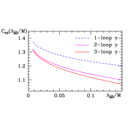
Figure 1: Conversion factor to the matching scheme that translates a RGI matrix element of $A^{\rm stat}_{0}$ at infinite mass to the one at finite mass. Its uncertainty is estimated to be smaller than 2% (half of the difference between the 2– and 3–loop results).

2.1 RGI matrix element in the static theory

As mentioned before, heavy-light correlation functions on the lattice, from which B-physics matrix elements such as the B-meson decay constant in question are obtained at large Euclidean time, are affected by large statistical errors in the static approximation. Their noise-to-signal ratio grows exponentially with the time separation, and in particular for the Eichten-Hill action stat:eichhill1 ,

$$S_{\rm h}=a^{4}\sum_{x}\overline{\psi}_{\rm h}(x)D_{0}\psi_{\rm h}(x)\,,$$ (4)

this ratio roughly behaves as $\exp\{x_{0}(E_{\rm stat}-m_{\pi})\}$ stat:hashi with $E_{\rm stat}$ the bare ground state energy of a B-meson in the static theory, diverging linearly in the continuum limit.

To overcome this difficulty, we introduced in Ref. fbstat:pap1 a few alternative discretizations of the static theory that retain the ${\rm O}(a)$ improvement properties of the action (4) but lead to a substantial reduction of the statistical fluctuations. These new static quark actions rely on changes of the parallel transporters $U(x,\mu)$ in the covariant derivative $D_{0}\psi_{\rm h}(x)=a^{-1}[\,\psi_{\rm h}(x)-U^{\dagger}(x-a\hat{0},0)\psi_{\rm h}(x-a\hat{0})\,]$ of the form $U(x,0)\rightarrow W(x,0)$, where now $W(x,0)$ is a function of the gauge fields in the immediate neighbourhood of $x,x+a\hat{0}$. Its best version employs ‘HYP-smearing’ that takes for $W(x,0)$ the so-called HYP-link, which is a function of the gauge links located within a hypercube HYP:HK01 . Comparing the noise-to-signal ratios in Figure 2, one can see that around $x_{0}\approx 1.5\,{\rm fm}$ more than an order of magnitude can be gained in this case w.r.t. to the Eichten-Hill action and, in addition, the statistical errors grow only slowly as $x_{0}$ is increased.

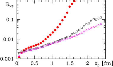
Figure 2: Noise-to-signal ratio of a B-meson correlation function in static approximation at $a\approx 0.08\,{\rm fm}$ for various actions fbstat:pap1 . Bullets refer to the original Eichten-Hill action, while triangles correspond to the alternative discretization with HYP-links.

Even more importantly, we observed fbstat:pap1 (see also lat03:statprec ) quite the same, small lattice artifacts with the new discretizations.

In our computational setup to determine the bare matrix element $\langle{\rm B}_{\rm s}|A^{\rm stat}_{0}|0\rangle$ entering eq. (1) we use the Schrödinger functional (SF) formulation of QCD with non-perturbatively ${\rm O}(a)$ improved Wilson actions in the gauge and light (i.e. relativistic) quark sectors. For technical details and the exact definitions of the correlation functions we refer to Refs. zastat:pap3 ; fbstat:pap1 . Here we only record that msbar:pap2

$$\langle\,{\rm B}_{\rm s}\,|\,A^{\rm stat}_{0}\,|\,0\,\rangle\propto\frac{f_{\rm A}^{\rm stat}(x_{0})}{\sqrt{f_{1}}}\,{\rm e}^{\,(x_{0}-T/2)E_{\rm stat}(x_{0})}\,,$$ (5)

modulo volume factors, where $f_{\rm A}^{\rm stat}$ is a proper SF correlation function of the (${\rm O}(a)$ improved) static axial current with the quantum numbers of a B-meson and $f_{1}$ is a corresponding boundary-to-boundary correlator, which serves to cancel the renormalization factors of the boundary quark fields. Moreover, we implement wave functions at the boundaries of the SF-cylinder to construct an interpolating B-meson field that suppresses unwanted contaminations from excited B-meson states to the correlators.

So far, the bare matrix element (5) has been calculated for three lattice spacings ($a$ $\approx$ $0.1\,{\rm fm}$, $0.08\,{\rm fm}$ and $0.07\,{\rm fm}$), and the regularization dependent part of the factor $Z_{\rm RGI}$, which according to (1) must be attached to get the RGI matrix element, has been computed for the new actions as it was done for the Eichten-Hill action in Ref. zastat:pap3 . The continuum extrapolation quadratic in the lattice spacing of our results stemming from the static action with HYP-links is displayed in the right part of Figure 3.

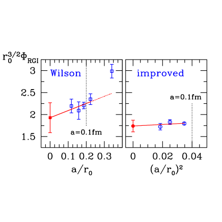
Figure 3: RGI matrix element of $A^{\rm stat}_{0}$ zastat:pap3 , based on unimproved bare data from stat:fnal2 ; stat:DMcN94 (left) and on simulations of the ${\rm O}(a)$ improved theory with the new discretization fbstat:pap1 ; lat03:statprec (right). A continuum extrapolation of the latter yields $r_{0}^{3/2}\Phi_{\rm RGI}=1.74(13)$.

To illustrate the gain in precision and control of the systematic errors, we confront our ${\rm O}(a)$ improved results with an analysis of older unimproved Wilson data for the bare matrix element, reproduced from zastat:pap3 in the left part of the figure.

2.2 Extrapolation in the heavy quark mass

To finally arrive at a value for $F_{\rm B_{\rm s}}$, we combine $\Phi_{\rm RGI}$, referring to the static limit and thus being independent of the heavy quark mass, with numbers of $F_{\rm PS}$ in the continuum limit at finite values of the quark mass, which have been collected in the context of the (quenched) computation of $F_{\rm D_{\rm s}}$ of fds:JR03 ; lat03:fds . In incorporating the mass dependence (2) predicted by HQET, we are then led to extrapolate $r_{0}^{3/2}F_{\rm PS}\sqrt{m_{\rm PS}}/C_{\rm PS}(M/\Lambda_{\overline{{\rm MS}}})$ from the charm region to the static estimate $r_{0}^{3/2}\Phi_{\rm RGI}$ by a linear fit in $1/(r_{0}m_{\rm PS})$. This interpolation is shown in Figure 4, where the zigzag error bands around the relativistic data indicate a small systematic effect that is due to the mass dependence of the discretization errors in the decay constant near the charm quark mass as discussed in Refs. lat03:fbstat ; lat03:fds . While an extrapolation in $1/(r_{0}m_{\rm PS})$ from the charm region without the constraint through the static approximation would look similar, it is obvious that the interpolation is much safer, since extrapolating to the (quite distant) ${\rm B}_{\rm s}$-meson scale depends significantly on the functional form assumed.

Using $m_{{\rm B}_{\rm s}}=5.4\,{\rm GeV}$, $r_{0}=0.5\,{\rm fm}$ and the numerical perturbative value of the matching factor $C_{\rm PS}(M_{\rm b}/\Lambda_{\overline{{\rm MS}}})$ translating to finite b-quark mass, we find from the interpolation to $1/(r_{0}m_{{\rm B}_{\rm s}})$ in Figure 4 as our present result lat03:fbstat

$$r_{0}F_{\rm B_{\rm s}}=0.52(3)\,\,\rightarrow\,\,F_{\rm B_{\rm s}}=206(10)\,{\rm MeV}\,.$$ (6)

This number includes all errors except for the quenched approximation; the (unavoidable) scale ambiguity introduced by it can be estimated to be about $12\%$.

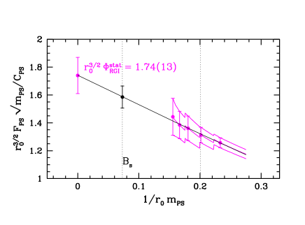
Figure 4: Interpolation in the inverse heavy-strange meson mass, $m_{\rm PS}$, between the RGI matrix element of the static axial current and relativistic data around the charm quark mass lat03:fbstat .

3 The b-quark’s mass

The second of the aforementioned problems that so far hampered the use of HQET on the lattice is the occurrence of power-law divergences in the lattice spacing. It already shows up in the static approximation and thereby affects, for instance, the computation of the mass of the b-quark in leading order of HQET. In this case the kinetic and the mass terms in the static action mix under renormalization and give rise to a local mass counterterm $\delta m\propto 1/a$, the self-energy of the static quark, which implies a linearly divergent truncation error if one relies on an only perturbative subtraction of this divergence. Therefore, past lattice computations in the framework of HQET could not reach the continuum limit lat01:ryan ; reviews:ichep02 .

A strategy for a solution to this longstanding problem was developed in Ref. mbstat:pap1 , which now offers the possibility to perform clean, non-perturbative calculations in HQET. It basically consists of three parts that I want to briefly describe in the following by sketching a (still ongoing) computation of the b-quark’s mass as example mbstat:pap1 ; mbstat:pap2 :

1. Renormalization of the effective theory amounts to relate the parameters of the HQET Lagrangian to those of QCD, a step usually called matching. In order to realize the matching in a non-perturbative way, one imposes matching conditions of the form $\Phi^{\rm HQET}(L_{0},M)=\Phi^{\rm QCD}(L_{0},M)$ in a physically small volume of linear extent $L_{0}={\rm O}(0.2\,{\rm fm})$, where $\Phi^{\rm HQET}$ and $\Phi^{\rm QCD}$ are suitably chosen observables in HQET and QCD to be calculated with the aid of numerical simulations. The finiteness of the matching volume ensures that lattice resolutions satisfying $am_{\rm b}\ll 1$ are possible and the b-quark can be treated as standard relativistic fermion, while at the same time the energy scale $1/L_{0}={\rm O}(1\,{\rm GeV})$ is still significantly below $m_{\rm b}$ and HQET applies quantitatively. In determining the parameters of the effective theory from those of QCD via such a non-perturbative matching in finite volume, the predictive power of QCD is transfered to HQET. Of course, owing to the very construction of the effective theory, it is clear that these matching conditions must also carry a dependence on the heavy quark mass, which is most conveniently identified with the (scheme and scale independent) RGI mass, $M$ (see e.g. msbar:pap1 ).

   In the concrete case of the b-quark mass computation, definite choices for the quantities $\Phi$ have to be made to formulate a sensible matching condition between the quark mass in the full, relativistic theory (QCD) and HQET. Those are $\Gamma(L,M_{\rm b})$, denoting the energy of a state with the quantum numbers of a B-meson but defined in a small volume of extent $L$, and $\Gamma_{\rm stat}(L)$ as its counterpart in (leading order of) the effective theory. As detailed in mbstat:pap1 ; QCDvsHQET:pap1 , both can be expressed as logarithmic derivatives of appropriate finite-volume, heavy- and static-light correlation functions, respectively, and numerically evaluated with high precision.

2. Next we need to establish a connection to a physical situation, where observables of the infinite-volume theory such as masses or matrix elements are accessible at the end. The accompanying gap between the small volume with its fine lattice resolution, where the matching of HQET and QCD is done, on the one side and larger lattice spacings (and also larger volumes) on the other is bridged by a recursive finite-size scaling procedure inspired by alpha:sigma : the volume to compute the quantity $\Gamma_{\rm stat}(L)$ in HQET is iteratively enlarged until one reaches a volume of linear extent $L={\rm O}(1\,{\rm fm})$ so that, at the same resolutions $a/L$ (i.e. at the same bare parameters) met there, large volumes with $L\approx 2\,{\rm fm}$ — to accommodate physical observables in the infinite-volume theory — eventually become affordable. Also note that, apart from terms of ${\rm O}(1/(L_{0}M_{\rm b})^{n+1})$ if considering HQET up to order $n$, any dependence on the unphysical small-volume physics is gone now.

3. Finally, a physical, dimensionful input is still missing. In the case at hand this means to link the energy $\Gamma_{\rm stat}$, which turns into the B-meson’s static binding energy, $E_{\rm stat}$, as the volume grows, to the mass of the B-meson as the physical observable in large volume whose numerical value is taken from experiment.

To join the foregoing three steps, we have to recall that energies in the effective theory differ from the corresponding ones in QCD by a linearly divergent mass shift $m_{\rm bare}$, which has its origin in the mixing of $\overline{\psi}_{\rm h}D_{0}\psi_{\rm h}$ with the lower-dimensional operator $\overline{\psi}_{\rm h}\psi_{\rm h}$ under renormalization — the central problem we started from. As a consequence of its universality (i.e. its independence of the state), however, $m_{\rm bare}$ obeys at any fixed lattice spacing

$$m_{\rm B} = E_{\rm stat}+m_{\rm bare}\,,$$ (7)

$$\Gamma(L,M_{\rm b}) = \Gamma_{\rm stat}(L)+m_{\rm bare}\,.$$ (8)

Imposing eq. (8) for $L=L_{0}$ as the non-perturbative matching condition in small volume implicitly determines the parameter $m_{\rm bare}$ and may hence be exploited to replace it in eq. (7). Then, after adding and subtracting a term $\Gamma_{\rm stat}(L_{2})$ (where $L_{2}=2^{2}L_{0}\approx 1\,{\rm fm}$ with lattice spacings commonly used in large-volume simulations), the resulting equation may be cast into the basic formula

$$m_{\rm B} \,=\, \underbrace{E_{\rm stat}-\Gamma_{\rm stat}(L_{2})}_{\scriptsize\mbox{$a\rightarrow 0$ in HQET}}\,+\,\underbrace{\Gamma_{\rm stat}(L_{2})-\Gamma_{\rm stat}(L_{0})}_{\scriptsize\mbox{$a\rightarrow 0$ in HQET}}$$

$$\,+\,\underbrace{\Gamma(L_{0},M_{\rm b})}_{\scriptsize\mbox{$a\rightarrow 0$ in QCD}}\,\,\,\,\,\,+\,\,\,\,\,\,{\rm O}\left(\Lambda^{2}/M_{\rm b}\right)$$

(with $\Lambda$ a typical low-energy QCD scale), where the terms are just arranged such that (the unknown) $m_{\rm bare}$ cancels in the energy differences $\Delta E\equiv E_{\rm stat}-\Gamma_{\rm stat}(L_{2})$ and $\Gamma_{\rm stat}(L_{2})-\Gamma_{\rm stat}(L_{0})$, and the continuum limit exists separately for each of the pieces entering eq. (3).

The entire heavy quark mass dependence is contained in $\Gamma(L_{0},M)$, defined in QCD with a relativistic b-quark. This mass dependence has been non-perturbatively mapped out in Ref. QCDvsHQET:pap1 , where as a particular ingredient of the numerical calculation, which demands to keep fixed the (dimensionless) RGI heavy quark mass while approaching the continuum limit, the knowledge of several renormalization factors and improvement coefficients relating the bare to the RGI quark mass is required. Although they had already been determined msbar:pap1 ; impr:babp , it was desirable to improve their precision and to estimate them directly in the bare coupling range relevant for our application.

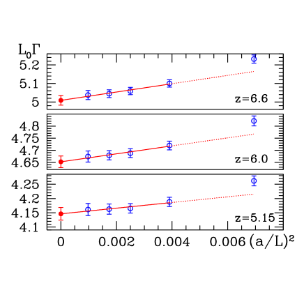
Figure 5: Continuum limit extrapolations of $L_{0}\Gamma(L_{0},M)$ in a relativistic QCD and small volume (of linear extent $L_{0}\approx 0.2\,{\rm fm}$) for representative values of $z\equiv L_{0}M$ QCDvsHQET:pap1 .

They were thus redetermined in QCDvsHQET:pap1 and, as exemplified in Figure 5, performing controlled continuum extrapolations provides $\omega\equiv\lim_{a/L\to 0}L_{0}\Gamma(L_{0},M)$ as function of $z\equiv L_{0}M$. In view of (3) the b-quark mass may now be extracted from the interception point of $\omega(z)$ with the combination

$$\omega_{\rm stat}\equiv L_{0}m_{\rm B}-L_{0}\left\{\Gamma_{\rm stat}(L_{2})-\Gamma_{\rm stat}(L_{0})\right\}-L_{0}\Delta E\,.$$ (10)

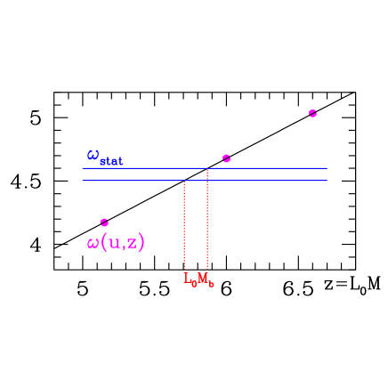
Figure 6: Solution of (3) for the dimensionless RGI b-quark mass, $L_{0}M_{\rm b}$. ($u$ indicates that during the computation one works at a certain fixed value of the renormalized SF coupling.)

The associated graph is given by Figure 6, where for the time being we restricted the analysis to unimproved Wilson fermion data for $aE_{\rm stat}$ from the literature stat:fnal2 , resulting in $L_{0}\Delta E=0.46(5)$ (cf. the l.h.s. of Figure 7). We presently obtain in static and quenched approximation mbstat:pap1

$$r_{0}M_{\rm b}=16.12(29)\,\,\rightarrow\,\,\overline{m}_{\rm b}^{\,\overline{\rm MS}}\big{(}\overline{m}_{\rm b}^{\,\overline{\rm MS}}\big{)}=4.12(8)\,{\rm GeV}$$ (11)

up to corrections of ${\rm O}(\Lambda^{2}/M_{\rm b})={\rm O}(\Lambda/(L_{0}M_{\rm b}))$. From the — yet preliminary — r.h.s. of Figure 7 fbstat:pap1 ; mbstat:pap2 one infers that, once the computation of $aE_{\rm stat}$ with the static action discussed above (which also has linear ${\rm O}(a)$ lattice artifacts removed) is finished, a continuum limit of $L_{0}\Delta E$ with a (by a factor $\approx 3$) smaller error is in sight and will substantially enhance the accuracy of the result (11).

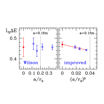
Figure 7: Subtracted, dimensionless ${\rm B}_{\rm s}$–meson energy evaluated from bare Wilson fermion numbers of stat:fnal2 (left) and from simulations with the alternative discretization of fbstat:pap1 ; mbstat:pap2 (right).

4 Conclusions and outlook

This status report on actual work of our collaboration makes evident that, by virtue of (mainly two) recent advances, non-perturbative calculations using the lattice regularized heavy quark effective theory have reached a new quality. One important ingredient is the use of a modified static action which, for the first time, enables to compute B-meson lattice correlation functions with good statistical precision in the static approximation for $x_{0}>1\,{\rm fm}$. As demonstrated both for the ${\rm B}_{\rm s}$-meson decay constant and for the b-quark mass, this represents a considerable improvement and has a great impact on the achievable precision in B-physics computations employing HQET. The determination of $\overline{m}_{\rm b}^{\,\overline{\rm MS}}$ also applies the other promising development, a general strategy how to solve renormalization problems in HQET entirely non-perturbatively, taking the continuum limit throughout all steps involved.

In the quenched approximation, where all the presented results refer to, the quoted uncertainties can (and will) be further reduced. Moreover, in interpolating between data obtained in QCD and in the static limit, our result for $F_{\rm B_{\rm s}}$ is almost independent of any effective theory.

Finally it is worth to emphasize the interesting potential of these methods for systematic and straightforward (albeit technically ambitious) extensions. Since it is one of the benefits of the theoretical concepts addressed here that describing the b-quark by an effective theory circumvents the need for prohibitively large lattices (because it completely eliminates the mass scale of the b-quark), they will very likely allow to also go beyond the static approximation by inclusion of $1/m_{\rm b}$–corrections as well as to incorporate dynamical fermions without major obstacles.

- (1) BABAR, J.J. Back, Nucl. Phys. Proc. Suppl. 121 (2003) 239, hep-ex/0308069; Belle, M. Yamauchi, Nucl. Phys. Proc. Suppl. 117 (2003) 83; HERA-B, A. Zoccoli, Nucl. Phys. A715 (2003) 280.
- (2) E. Eichten and B. Hill, Phys. Lett. B234 (1990) 511.
- (3) L. Maiani, G. Martinelli and C.T. Sachrajda, Nucl. Phys. B368 (1992) 281.
- (4) ALPHA, M. Della Morte et al., (2003), hep-lat/0307021.
- (5) ALPHA, J. Rolf et al., (2003), hep-lat/0309072.
- (6) ALPHA, J. Heitger and R. Sommer, Nucl. Phys. Proc. Suppl. 106 (2002) 358, hep-lat/0110016.
- (7) ALPHA, J. Heitger and R. Sommer, (2003), hep-lat/0310035.
- (8) ALPHA, J. Heitger, M. Kurth and R. Sommer, Nucl. Phys. B669 (2003) 173, hep-lat/0302019.
- (9) R. Sommer, Nucl. Phys. Proc. Suppl. 119 (2003) 185, hep-lat/0209162.
- (10) K.G. Chetyrkin and A.G. Grozin, Nucl. Phys. B666 (2003) 289, hep-ph/0303113.
- (11) S. Hashimoto, Phys. Rev. D50 (1994) 4639, hep-lat/9403028.
- (12) A. Hasenfratz and F. Knechtli, Phys. Rev. D64 (2001) 034504, hep-lat/0103029.
- (13) ALPHA, M. Della Morte et al., (2003), hep-lat/0309080.
- (14) ALPHA, M. Guagnelli et al., Nucl. Phys. B560 (1999) 465, hep-lat/9903040.
- (15) A. Duncan et al., Phys. Rev. D51 (1995) 5101, hep-lat/9407025.
- (16) T. Draper and C. McNeile, Nucl. Phys. Proc. Suppl. 34 (1994) 453, hep-lat/9401013.
- (17) ALPHA, A. Jüttner and J. Rolf, Phys. Lett. B560 (2003) 59, hep-lat/0302016.
- (18) A. Jüttner and J. Rolf, (2003), hep-lat/0309069.
- (19) S.M. Ryan, Nucl. Phys. Proc. Suppl. 106 (2002) 86, hep-lat/0111010.
- (20) L. Lellouch, Nucl. Phys. Proc. Suppl. 117 (2003) 127, hep-ph/0211359.
- (21) ALPHA, in preparation.
- (22) ALPHA, S. Capitani et al., Nucl. Phys B544 (1999) 669, hep-lat/9810063.
- (23) J. Heitger and J. Wennekers, in preparation.
- (24) M. Lüscher, P. Weisz and U. Wolff, Nucl. Phys. B359 (1991) 221.
- (25) ALPHA, M. Guagnelli et al., Nucl. Phys. B595 (2001) 44, hep-lat/0009021.
- (26) G.M. de Divitiis et al., (2003), hep-lat/0305018.
- (27) G.M. de Divitiis et al., (2003), hep-lat/0307005.