RHIC Physics: The Quark Gluon Plasma and The Color Glass Condensate: 4 Lectures

Abstract

The purpose of these lectures is to provide an introduction to the physics issues which are being studied in the RHIC heavy ion program. These center around the production of new states of matter. The Quark Gluon Plasma is thermal matter which once existed in the big bang which may be made at RHIC. The Color Glass Condensate is a universal form of matter which controls the high energy limit of strong interactions. Both such forms of matter might be produced and probed at RHIC.

1 Introduction

These lectures will introduce the listener to the physics issues behind the experimental heavy ion program at RHIC. This program involves the collisions of protons on protons, deuterons on nuclei, and nuclei on nuclei. The collision energy is of order 200 GeV per nucleon in the center of mass. The goal of these experimental studies is to produce new forms of matter. This may be a Quark Gluon Plasma or a Color Glass Condensate. The properties of these forms of matter are described below.

The outline of these lectures is

• New States of Matter
  In the first lecture I describe the new forms of matter which may be produced in heavy ion collisions. These are the Quark Gluon Plasma and the Color Glass Condensate.

• Space Time Dynamics
  This lecture describes the space-time dynamics of high energy heavy ion collisions. In this lecture, I illustrate how high energy density matter might be formed.

• Experiment and Theory
  In this lecture, I show how various experimental measurements might teach us about the properties of matter.

• The Color Glass Condensate
  In this lecture, some aspects of the Color Glass Condensate are developed, in particular the renormalization group equations.

2 Lecture I: High Density Matter

2.1 The Goals of RHIC

The goal of nuclear physics has traditionally been to study matter at densities of the order of those in the atomic nucleus,

$$\epsilon\sim.15~{}GeV/Fm^{3}$$ (1)

High energy nuclear physics has extended this study to energy densities several orders of magnitude higher. This extension includes the study of matter inside ordinary strongly interacting particles, such as the proton and the neutron, and producing new forms of matter at much higher energy densities in high energy collisions of nuclei with nuclei, and various other probes.

RHIC is a multi-purpose machine which can address at least three central issues of high energy nuclear physics. These are:

• The production of matter at energy densities one to two orders of magnitude higher than that of nuclear matter and the study of its properties.
  This matter is at such high densities that it is only simply described in terms of quarks and gluons and is generically referred to as the Quark Gluon Plasma. The study of this matter may allow us to better understand the origin of the masses of ordinary particles such as nucleons, and of the confinement of quarks and gluons into hadrons. The Quark Gluon Plasma will be described below.[1]

• The study of the matter which controls high energy strong interactions.
  This matter is believed to be universal (independent of the hadron), and exists over sizes large compared to the typical microphysics size scales important for high energy strong interactions. (The microphysics size scale here is about $1~{}Fm$ and the microphysics time scale is the time it takes light to fly $1~{}Fm$, $t\sim 10^{-23}~{}sec$.) It is called a Color Glass Condensate because it is composed of colored particles, evolves on time scales long compared to microphysics time scales and therefore has properties similar to glasses, and a condensate since the phase space density of gluons is very high. The study of this matter may allow us to better understand the typical features of strong interactions when they are truly strong, a problem which has eluded a basic understanding since strong interactions were first discovered. The Color Glass Condensate will be described below.[2]

• The study of the structure of the proton, most notably spin.
  

  The structure of the proton and neutron is important as these particles form the ordinary matter from which we are composed. We would like to understand how valence quantum numbers such as baryon number, charge and spin are distributed. RHIC has an active program to study the spin of the proton.[3]

Because I was asked to provide lectures on the heavy ion program at RHIC, I shall discuss only the first two issues.

2.2 The Quark Gluon Plasma

This section describes what is the Quark Gluon Plasma, why it is important for astrophysics and cosmology, and why it provides a laboratory in which one can study the origin of mass and of confinement.[1]

2.2.1 What is the Quark Gluon Plasma?

Matter at low energy densities is composed of electrons, protons and neutrons. If we heat the system, we might produce thermal excitations which include light mass strongly interacting particles such as the pion. Inside the protons, neutrons and other strongly interacting particles are quarks and gluons. If we make the matter have high enough energy density, the protons, nucleons and other particles overlap and get squeezed so tightly that their constituents are free to roam the system without being confined inside hadrons.[4] At this density, there is deconfinement and the system is called a Quark Gluon Plasma. This is shown in Fig. 1

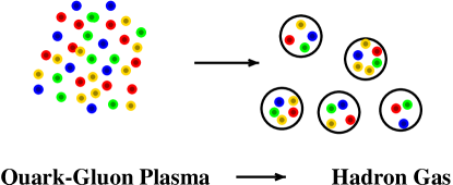
Figure 1: As the energy density is decreased, the Quark Gluon Plasma condenses into a low density gas of hadrons. Quarks are red, green or blue and gluons are yellow.

As the energy density gets to be very large, the interactions between the quarks and gluons become weak. This is a consequence of the asymptotic freedom of strong interactions: At short distances the strong interactions become weak.

The Quark Gluon Plasma surely existed during the big bang. In Fig 2, the various stages of evolution in the big bang are shown.

Figure 2: The various forms of matter, and the types of physics which are probed during the big bang.

At the earliest times in the big bang, temperatures are of order $T\sim 10^{19}~{}GeV$, quantum gravity is important, and despite the efforts of several generations of string theorists, we have little understanding. At somewhat lower temperatures, perhaps there is the grand unification of all the forces, except gravity. It might be possible that the baryon number of the universe is generated at this temperature scale. At much lower temperatures, of order $T\sim 100~{}GeV$, electroweak symmetry breaking takes place. It is possible here that the baryon asymmetry of the universe might be produced. At temperatures of order $T\sim 1~{}GeV$, quarks and gluons become confined into hadrons. This is the temperature range RHIC is designed to study. At $T\sim 1~{}MeV$, the light elements are made. This temperature corresponds to an energy range which has been much studied, and is the realm of conventional nuclear physics. At temperatures of the order of an electron volt, corresponding to the binding energies of electrons in atoms, the universe changes from an ionized gas to a lower pressure gas of atoms, and structure begins to form.

The Quark Gluon Plasma is formed at energy densities of order $1~{}GeV/Fm^{3}$. Matter at such energy densities probably exists inside the cores of neutron stars as shown in Fig. 3.

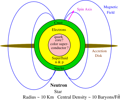
Figure 3: A spinning neutron star

Neutron stars are objects of about $10~{}Km$ in radius and are composed of extremely high energy density matter. The typical energy density in the core is of the order of $1~{}GeV/Fm^{3}$, and approaches zero at the surface. Unlike the matter in the big bang, this matter is cold and has temperature small compared to the Fermi energies of quarks. It is a cold, degenerate gas of quarks. At lower densities, this matter converts into a cold gas of nucleons.

Hot and dense matter with energy density of order $1~{}GeV/Fm^{3}$ may have occurred in the supernova explosion which led to the neutron star’s formation. It may also occur in collisions of neutron stars and black holes, and may be the origin of the mysterious gamma ray bursters. (Gamma ray bursters are believed to be starlike objects which convert of the order of their entire mass in to gamma rays.)

2.2.2 The Quark Gluon Plasma and Ideal Gasses

At very high energy temperatures, the coupling constant of QCD becomes weak. A gas of particles should to a good approximation become an ideal gas. Each species of particle contributes to the energy density of an ideal gas as

$$\epsilon=\int{{d^{3}p}\over{(2\pi)^{3}}}\sum_{i}{E_{i}\over{e^{\beta E_{i}}\pm 1}}$$ (2)

where the $-$ is for Bosons and the $+$ for Fermions. The energy of each particle is $E_{i}$. At high temperatures, masses can be ignored, and the factor of $\pm 1$ in the denominator turns out to make a small difference. One finds therefore that

$$\epsilon\sim{\pi^{2}\over{30}}NT^{4}$$ (3)

where $N$ is the number of particle degrees of freedom. At low temperatures when masses are important, only the lowest mass strongly interacting particle degree of freedom contributes, the pion, and the energy density approaches zero as $\epsilon\sim e^{-m_{\pi}/T}$. For an ideal gas of pions, the number of pion degrees of freedom are three. For a quark gluon plasma there are two helicities and eight colors for each gluon, and for each quark, three colors, 2 spins and a quark-antiquark pair. The number of degrees of freedom is $N\sim 2\times 8+4\times 3\times N_{F}$ where $N_{F}$ is the number of important quark flavors, which is about $3$ if the temperature is below the charm quark mass  so that $N\sim 50$.

There is about an order of magnitude change in the number of degrees of freedom between a hadron gas and a Quark Gluon Plasma. This is because the degrees of freedom of the QGP include color. In the large $N_{color}$ limit, the number of degrees of freedom of the plasma are proportional to $N_{color}^{2}$, and in the confined phase is of order $1$. In this limit, the energy density has an infinite discontinuity at the phase transition. There would be a limiting temperature for the hadronic world in the limit for which $N_{color}\rightarrow\infty$, since at some temperature the energy density would go to infinity. This is the Hagedorn limiting temperature. (In the real world $N_{color}$ is three, and there is a temperature at which the energy density changes by an order of magnitude in a narrow range.)

2.2.3 The Quark Gluon Plasma and Fundamental Physics Issues

The nature of matter at high densities is an issue of fundamental interest. Such matter occurred during the big bang, and it is the ultimate and universal state of matter at very high energy densities.

A hypothetical phase diagram for QCD is shown in Fig. 4. The vertical axis is temperature, and the horizontal is a measure of the matter or baryon number density, the baryon number chemical potential.[5] The solid lines indicate a first order phase transition, and the dashed line a rapid cross over. It is not known for sure whether or not the region marked cross over is or is not a true first order phase transition. There are analytic arguments for the properties of matter at high density, but numerical computation are of insufficient resolution. At high temperature and fixed baryon number density, there are both analytic arguments and numerical computations of good quality. At high density and fixed temperature, one goes into a superconducting phase, perhaps multiple phases of superconducting quark matter. At high temperature and fixed baryon number density, the degrees of freedom are those of a Quark Gluon Plasma.

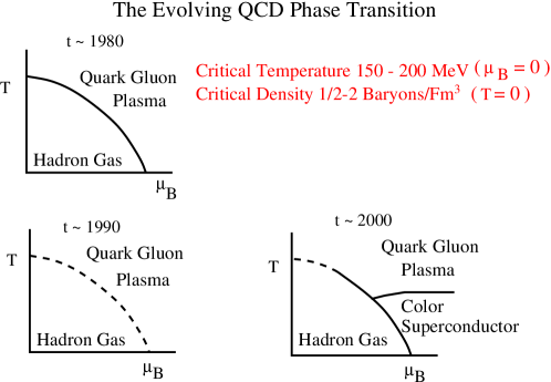
Figure 4: A phase diagram for QCD collisions.

I have shown this phase diagram as a function of time. What this means is that at various times people thought they knew what the phase diagram was. As time evolved, the picture changed. The latest ideas are marked with the date 2000. The point of doing this is to illustrate that theoretical ideas in the absence of experiment change with time. Physics is essentially an experimental science, and it is very difficult to appreciate the richness which nature allows without knowing from experiment what is possible.

Much of the information we have about QCD at finite energy density comes from lattice gauge theory numerical simulation.[5] To see how lattice gauge theory works, recall that at finite temperature, the Grand Canonical Ensemble is given by

$$Z=Tr~{}e^{-\beta H}$$ (4)

This is similar to computing

$$Z=<e^{-itH}>$$ (5)

where $-it=\beta$. That is we compute the expectation value of the time evolution operator for imaginary time. This object has a path integral representation, which has been described to you in your elementary field theory text books. Under the change of variables, the action becomes $iS=i\int dtL\rightarrow S=-\int_{0}^{\beta}d\tau L$. Here $L$ is the Lagrangian.

The Grand Canonical Ensemble has the representation

$$Z=\int[dA]e^{-S[A]}$$ (6)

for a system of pure gluons. The gluon fields satisfy periodic boundary conditions due to the trace in the definition of the Grand Canonical Ensemble. (Fermions may also be included, although the path integral is more complicated, and the fermion fields are required to satisfy antiperiodic boundary conditions.) Expectation values are computed as

$$<0>={{Tr~{}Oe^{-\beta H}}\over{Tr~{}e^{-\beta H}}}$$ (7)

The way that lattice Monte Carlo simulates the Grand Canonical Ensemble is by placing all of the fields on a finite grid, so the path integral becomes finite dimensional. Then field configurations are selectively sampled, as weighted by their action. This works because the factor of $e^{-\beta H}$ is positive and real. (The method has essential complications for finite density systems, since there the action becomes complex.)

Lattice gauge theory numerical studies, and analytic studies have taught us much about the properties of these various phases of matter.[5] There have been detailed computations of the energy density as a function of temperature. In Fig. 5

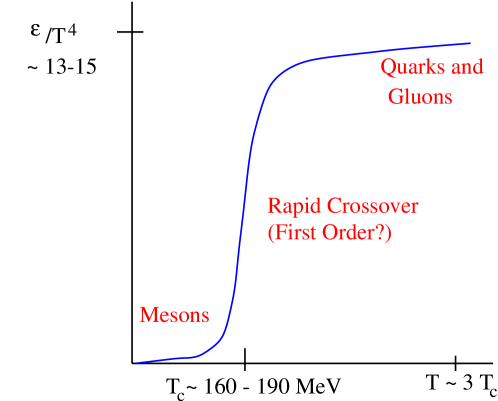
Figure 5: The energy density scaled by $T^{4}$ as a function of temperature.

the energy density scaled by $T^{4}$ is plotted. This is essentially the number of degrees of freedom of the system as function of $T$. At a temperature of $T_{c}\sim 160-190~{}MeV$ the number of degrees of freedom changes very rapidly, possibly discontinuously. This is the location of the transition from the hadron gas to the quark gluon plasma.

In Fig. 6, the sound velocity is plotted as

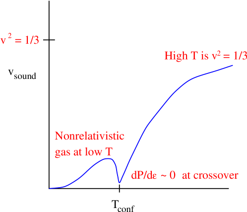
Figure 6: The sound velocity as a function of temperature.

a function of temperature. The sound velocity increases at high temperature asymptoting to its ideal gas value of $v_{sound}^{2}\sim 1/3$. Near the phase transition, it become very small. This is because the energy density jumps at the transition temperature, but the pressure must be smooth and continuous. The sound velocity squared is $d\epsilon/dP$.

Lattice Monte-Carlo simulation has also studied how the phase transition is related to the confining force. In a theory with only gluons, the potential for sources of fundamental representation color charge grows linearly in the confined phase. (With dynamical fermions, the potential stops rising at some distance when it is energetically favorable to produce quark-antiqaurk pairs which short out the potential.)

We can understand how confinement might disappear at high temperature. A finite temperature, there is a symmetry of the pure gluon Yang-Mills system. Consider a Wilson line which propagates from $(0,\vec{x})$ to the point $(\beta,\vec{x})$ A wilson line is a path ordered phase,

$$L(x)=P\exp{\int_{0}^{\beta}dtA^{0}(t,\vec{x})}$$ (8)

One can show that the expectation value of this line gives the free energy of an isolated quark:

$$e^{-\beta F}={1\over N_{c}}<tr(L(x))>$$ (9)

Now consider gauge transformations which maintain the periodic boundary conditions on the gauge fields (required by the trace in the definition of the Grand Canonical Ensemble). The most general gauge transformation which does this is not periodic but solves

$$U(\beta,\vec{x})=ZU(0,\vec{x})$$ (10)

One can show that $[z,\tau^{a}]=0$, and that $\nabla^{i}Z=0$. $Z$ is an element of the gauge group so that $detZ=1$. These conditions require that

$$Z=e^{2\pi ij/N_{c}}$$ (11)

This symmetry under non-periodic gauge transformations is global, that is it does not depend upon the position in space. It may be broken. If it is realized, the free energy of a quark must be infinite since $L\rightarrow ZL$ under this transformation, and $<L>=0$. If the symmetry is broken, quarks can be free.

Lattice gauge computations have measured the quark-antiquark potential as a function of $T$, and at the deconfinement temperature, the potential changes from linear at infinity to constant. This is shown in Fig. 7.

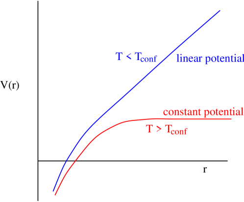
Figure 7: The potential in pure gauge theory as a function of temperature.

In addition to confinement-deconfinement, there is an additional symmetry which might become realized at high temperatures. In nature, the up and down quark masses are almost zero. This leads to a chiral symmetry, which is the rotation of fermion fields by $e^{i\gamma_{5}\theta}$. This symmetry if realized would require that either baryons are massless or occur in parity doublets. Neither is realized in nature. The nucleon has a mass of about $1~{}GeV$ and has no opposite parity partner of almost equal mass. It is believed that this symmetry becomes broken, and as a consequence, the nucleon acquires mass, and that the pion becomes an almost massless Goldstone boson. It turns out that at the confinement-deconfinement phase transition, chiral symmetry is restored. This is seen in Fig. 8, where a quantity proportional to the nucleon mass is plotted as a function of T.

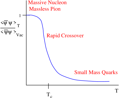
Figure 8: The chiral order parameter $<\overline{\Psi}\Psi>$ as a function of temperature.

The chiral symmetry restoration phase transition can have interesting dynamical consequences. In the confined phase, the mass of a nucleon is of order $N_{c}\Lambda_{QCD}$, but in the deconfined phase is of order $T$. Therefore in the confined phase, the Boltzman weight $e^{-M/T}$ is very small. Imagine what happens as we go through the phase transition starting at a temperature above $T_{c}$. At first the system is entirely in QGP. As the system expands, a mixed phase of droplets of QGP and droplets of hadron gas form. The nucleons like to stay in the QGP because their Boltzman weight is larger. As the system expands further, the droplets of QGP shrink, but most of the baryon number is concentrated in them. At the end of the mixed phase, one has made large scale fluctuations in the baryon number. This scenario is shown in Fig. 9

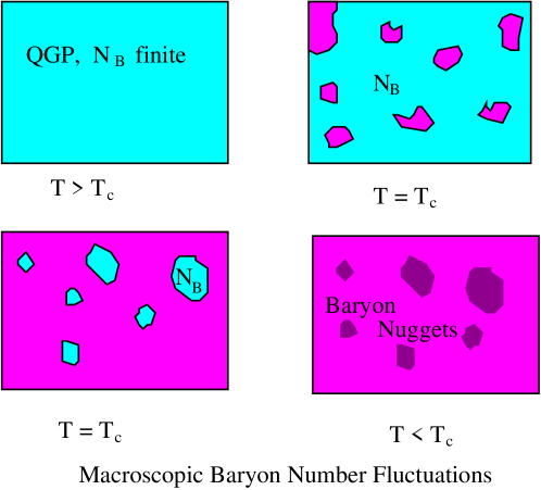
Figure 9: Formation of large scale baryon number fluctuations at the QCD phase transition.

The confinement-deconfinement phase transition and the chiral symmetry restoration phase transition might be logically disconnected from one another. The confinement-deconfinement phase transition is related to a symmetry when the quark masses are infinite. The chiral transition is related to a symmetry when the quarks are massless. As a function of mass, one can follow the evolution of the phase transitions. At large and small masses there is a real phase transition marked by a discontinuity in physical quantities. At intermediate masses, there is probably a rapid transition, but not a real phase transition. It is believed that the real world has masses which make the transition closer to a crossover than a phase transition, but the evidence from lattice Monte-Carlo studies is very weak. In Fig. 10, the various possibilities are shown.

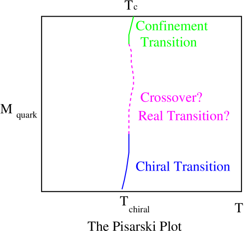
Figure 10: The phase diagram of QCD as a function of fermion mass.

2.3 The Color Glass Condensate

This section describes what is the Color Glass Condensate, and why it is important for our understanding of basic properties of strong interactions.[2],[6] I argue that the Color Glass Condensate is a universal form of matter which controls the high energy limit of all strong interaction processes and is the part of the hadron wavefunction important at such energies. Since the Color Glass Condensate is universal and controls the high energy limit of all strong interactions, it is of fundamental importance.

2.3.1 What is the Color Glass Condensate?

The Color Glass Condensate is a new form of matter which controls the high energy limit of strong interactions. It is universal and independent of the hadron which generated it. It should describe

• High energy cross sections

• Distributions of produced particles

• The distribution of the small x particles in a hadron

• Initial conditions for heavy ion collisions

Because this matter is universal, it is of fundamental interest.

A very high energy hadron has contributions to its wavefunction from gluons, quarks and anti-quarks with energies up to that of the hadron and all the way down to energies of the order of the scale of light mass hadron masses, $E\sim 200~{}MeV$. A convenient variable in which to think about these quark degrees of freedom is the typical energy of a constituent scaled by that of the hadron,

$$x=E_{constituent}/E_{hadron}$$ (12)

Clearly the higher the energy of the hadron we consider, the lower is the minimum $x$ of a constituent. Sometimes it is also useful to consider the rapidity of a constituent which is $y\sim ln(1/x)$

The density of small x partons is

$${{dN}\over{dy}}=xG(x,Q^{2})$$ (13)

The scale $Q^{2}$ appears because the number of constituents one measures depends (weakly) upon the resolution scale of the probe with which one measures. (Resolution scales are measured in units of the inverse momentum of the probe, which is usually taken to be a virtual photon.) A plot of $xG(x,Q^{2})$ for gluons at various $x$ and $Q^{2}$ measured at the HERA accelerator in protons[7], and is shown in Fig. 11.

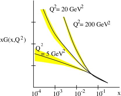
Figure 11: The number of gluons in a proton per unit rapidity at various rapidities and $Q^{2}$ resolutions.

Note that the gluon density rises rapidly at small x in Fig. [7]. This is the so called small x problem. It means that if we view the proton head on at increasing energies, the low momentum gluon density grows. This is shown in Fig. 12.

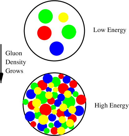
Figure 12: The increasing density of wee partons as the energy increases.

As the density of gluons per unit area per unit rapidity increases, the typical transverse separation of the gluons decreases. This means that the matter which controls high energy strong interactions is very dense, and it means that the QCD interaction strength, which is usually parameterized by the dimensionless scale $\alpha_{S}$ becomes small. The phase space density of these gluons, $\rho\sim 1/\pi R^{2}~{}dN/d^{2}p_{T}$ can become at most $1/\alpha_{s}$ since once this density is reached gluon interactions are important. This is characteristic of Bose condensation phenomena which are generated by an instability proportional to the density $\rho$ and is compensated by interactions proportional to $\alpha_{S}\rho^{2}$, which become of the same order of magnitude when $\rho\sim 1/\alpha_{s}$ Thus the matter is a Color Condensate.

The glassy nature of the condensate arises because the fields associated with the condensate are generated by constituents of the proton at higher momentum. These higher momentum constituents have their time scales Lorentz time dilated relative to those which would be measured in their rest frame. Therefore the fields associated with the low momentum constituents also evolve on this long time scale. The low momentum constituents are therefore glassy: their time evolution scale is unnaturally long compared to their natural time scale. Hence the name Color Glass Condensate.

There is also a typical scale associated with the Color Glass Condensate: the saturation momentum. This is the typical momentum scale where the phase space density of gluons becomes $\rho\leq 1/\alpha_{S}$.

At very high momentum, the fields associated with the Color Glass Condensate can be treated as classical fields, like the fields of electricity and magnetism. Since they arise from fast moving partons, they are plane polarized, with mutually orthogonal color electric and magnetic fields perpendicular to the direction of motion of the hadron. They are also random in two dimensions. This is shown in Fig. 13.

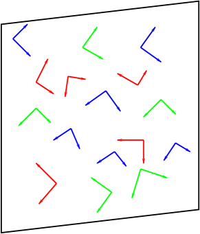
Figure 13: The Color Glass Condensate as a high density of random gluon fields on a two dimensional sheet traveling near the speed of light.

2.3.2 Why is the Color Glass Condensate Important?

Like nuclei and electrons compose atoms, and nucleons and protons compose nuclear matter, the Color Glass Condensate is the fundamental matter of which high energy hadrons are composed. The Color Glass Condensate has the potential to allow for a first principles description of the gross or typical properties of matter at high energies. For example, the total cross section at high energies for proton-proton scattering, as shown in Fig. 14 has a simple form but for over 40 years has resisted simple explanation. (It has perhaps been recently understood in terms of the Color Glass Condensate or Saturation ideas.)[8]-[11]

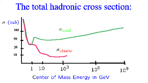
Figure 14: The total cross section for high energy proton-proton interactions.

The Color Glass Condensate forms the matter in the quantum mechanical state which describes a nucleus. In the earliest stages of a nucleus-nucleus collisions, the matter must not be changed much from these quantum mechanical states. The Color Glass Condensate therefore provides the initial conditions for the Quark Gluon plasma to form in these collisions. A space-time picture of nucleus nucleus collisions is shown in Fig. 15. At very early times, the Color Glass Condensate evolves into a distribution of gluons. Later these gluons thermalize and may eventually form a Quark Gluon Plasma. At even later times, a mixed phase of plasma and hadronic gas may form.

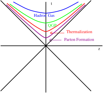
Figure 15: A space-time diagram for the evolution of matter produced in heavy ion collisions.

3 Lecture II: Ultrarelativistic Nuclear Collisions.

Heavy ion collisions at ultrarelativistic energies are visualized in Fig. 23 as the collision of two sheets of colored glass.[12]

At ultrarelativistic energies, these sheets pass through one another. In their wake is left melting colored glass, which eventually materializes as quarks and gluons. These quarks and gluons would naturally form in their rest frame on some natural microphysics time scale. For the saturated color glass, this time scale is of order the inverse saturation momentum (again, we convert momentum into time by appropriate uses of Planck’s constant and the speed of light), in the rest frame of the produced particle. When a particle has a large momentum along the beam axis, this time scale is Lorentz dilated. This means that the slow particles are produced first towards the center of the collision regions and the fast particles are produced later further away from the collision region.

Figure 16: The collision of two sheets of colored glass.

This correlation between space and momentum is similar to what happens to matter in Hubble expansion in cosmology. The stars which are further away have larger outward velocities. This means that this system, like the universe in cosmology is born expanding. This is shown in Fig. 17

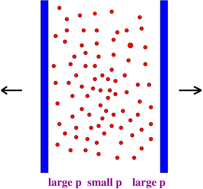
Figure 17: Particles being produced after the collision of two nuclei.

As this system expands, it cools. Presumably at some time the produced quarks and gluons thermalize, They then expand as a quark gluon plasma and eventually as some mixture of hadrons and quarks and gluons. Eventually, they may become a gas of only hadrons before they stop interacting and fly off to detectors.

In the last lecture, we shall describe the results from nucleus-nucleus collisions at RHIC in some detail. Before proceeding there, we need to learn a little bit more about the properties of high energy hadrons. It is useful to introduce some kinematic variables which are useful in what will follow.

The light cone momenta are defined as

$$P^{\pm}={1\over{\sqrt{2}}}(E\pm p_{z})$$ (14)

and light cone coordinates are

$$X^{\pm}={1\over{\sqrt{2}}}(t\pm z)$$ (15)

The metric in these variables is

$$p\cdot x=p^{+}x^{-}+p^{-}x^{+}-p_{T}\cdot x_{T}$$ (16)

Conjugate variables are $x^{\pm}<->p^{\mp}$. The square of the four momentum is

$$p^{2}=2P^{+}P^{-}-P_{T}^{2}=M^{2}$$ (17)

The uncertainty principle is

$$\Delta x^{\pm}\Delta p^{\mp}\geq 1$$ (18)

A reason why light cone variables are useful is because in a high energy collision, a left moving particle has $p_{Z}\sim E$, so that $p^{+}\sim\sqrt{2}E$, but $p^{-}\sim m_{T}^{2}/p_{z}\sim 0$. For the right moving particles, it is $p^{-}$ which is big and $p^{+}$ which is very small.

Light cone variables scale by a constant under Lorentz transformations along the collision axis. Ratios of light cone momentum are therefore invariant under such Lorentz boosts. The light cone momentum fraction $x=p^{+}_{i}/P^{+}$, where $P^{+}$ is that of the particle we probe and $p_{i}^{+}$ is that of the constituent of the probed hadron satisfies $0\leq x\leq 1$. It is the same as Bjorken x, and for a fast moving hadron, it is almost Feynman $x_{Feynman}=E_{i}/E$. This is the $x$ variable one is using when one describes deep inelastic scattering. In this case the label $i$ corresponds to a quark or gluon constituent of a hadron.

One can also define a rapidity variable:

$$y={1\over 2}ln\left\{p_{i}^{+}\over p_{i}^{-}\right\}\sim ln(2E_{i}/M_{T})$$ (19)

Up to mass effects, the rapidity is in the range $-y_{proj}\leq y\leq y_{proj}$ When particles, like pions, are produced in high energy hadronic collisions, one often plots them in terms of the rapidity variable. Distributions tend to be slowly varying functions of rapidity.

3.1 Is There Simple Behaviour at High Energy?

A hint of the underlying simplicity of high energy hadronic interactions comes from studying the rapidity distributions of produced particles for various collision energies. In Fig. 18,

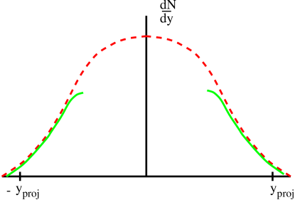
Figure 18: The rapidity distributions of particles at two different energies.

a generic plot of of the rapidity distribution of produced pions is shown for two different energies. The rapidity distribution at lower energies has been cut in half and the particles associated with each of the projectiles have been displaced in rapidity so that their staring points in rapidity are the same. It is remarkable, that except for the slowest particles in the center of mass frame, those located near $y\sim 0$, the distributions are almost identical.[13] This is shown for the data from RHIC in Fig. 19.

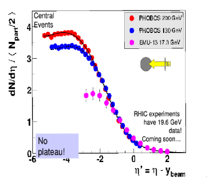
Figure 19: Experimental evidence from the Phobos experiment at RHIC on limiting fragmentation.

We conclude from this that going to higher energy adds in new degrees of freedom, the small x part of the hadron wavefunction. At lower energies, these degrees of freedom are not kinematically relevant as they can never be produced. On the other hand, going to higher energy leaves the fast degrees of freedom of the hadron unchanged.

This suggests that there should be a renormalization group description of the hadrons. As we go to higher energy, the high momentum degrees of freedom remain fixed. Integrating out the previous small x degrees of freedom should incorporate them into what are now the high energy degrees of freedom at the higher energy. This process generates an effective action for the new low momentum degrees of freedom. Such a process, when done iteratively is a renormalization group.

3.2 A Single Hadron

A plot of the rapidity distribution of the constituents of a hadron, the gluons, is shown generically in Fig. 20.

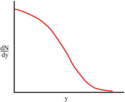
Figure 20: The rapidity distribution of the constituents of a hadron.

I have used $y=y_{hadron}-ln(1/x)$ as my definition of rapidity. This distribution is similar in shape to that of the half of the rapidity distribution shown for hadron-hadron interactions in the center of mass frame which has positive rapidity. The essential difference is that this distribution is for constituents where the hadron-hadron collision is for produced particles, mainly pions.

In the high energy limit, as discussed in the previous section, the density of gluons grows rapidly. This suggests we introduce a density scale for the partons

$$\Lambda^{2}={1\over{\pi R^{2}}}{{dN}\over{dy}}$$ (20)

One usually defines a saturation momentum to be $Q_{sat}^{2}\sim\alpha_{s}\Lambda^{2}$, since this will turn out to be the typical momentum of particles in this high density system. In fact, $\alpha_{s}$ is slowly varying compared to the variation of $\lambda$, so that for the purposes of the estimates we make here, whether or not there is a factor of $\alpha_{s}$ will not be so important. Note that $\alpha_{s}$ evaluated at the saturation scale will be $\alpha_{s}<<1$. The typical particle transverse momenta are of order $p_{T}^{2}\sim Q_{sat}^{2}>>1/R_{had}^{2}$ Therefore it is consistent to think of the parton distribution as a high density weakly coupled system which is localized in the transverse plane. The high momentum partons, the degrees of freedom which should be frozen, can be thought of as sitting on an infinitesmally thin sheet. We shall study this system with a resolution size scale which is $\Delta x<<1/\Lambda_{QCD}$, so that we may use weak coupling methods. Such a thin sheet is shown in Fig. 21

Figure 21: A thin sheet traveling near light velocity. The transverse resolution scale is $\Delta x$

It is useful to discuss different types of rapidity variables before proceeding. The typical momentum space rapidity is

$$y = {1\over 2}ln\left(p^{+}\over p^{-}\right)$$ (21)

$$= ln\left({2p^{+}}\over M_{T}\right)$$

$$= ln\left({2p^{+}_{hadron}}\over M_{T}\right)+ln\left(p^{+}\over p^{+}_{hadron}\right)$$

$$= y_{hadron}-ln(1/x)$$

Here $M_{T}$ is a particle transverse mass, and we have made approximations which ignore overall shifts in rapidity by of order one unit. Within these approximations, the momentum space rapidity used to describe the production of particles is the same as that used to describe the constituents of hadrons.

Oftentimes a coordinate space rapidity is introduced. With $\tau=\sqrt{t^{2}-z^{2}}$,

$$y={1\over 2}ln\left(x^{+}\over x^{-}\right)=ln(2\tau/x^{-})$$ (22)

Taking $\tau$ to be a time scale of order $1/M_{T}$, and using the uncertainty principle $x^{\pm}\sim 1/p^{\mp}$, we find that up to shifts in rapidity of order one, all the rapidities are the same. This implies that coordinate space and momentum space are highly correlated, and that one can identify momentum space and coordinate space rapidity with some uncertainty of order one unit.

If we plot the distribution of particles in hadron in terms of the rapidity variable, the longitudinal dimension of the sheet is spread out. This is shown in Fig. 22.

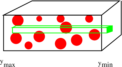
Figure 22: The distribution of particles in a hadron in terms of rapidity variables.

The longitudinal position is correlated with the longitudinal momentum. The highest rapidity particles are the fastest. In ordinary coordinate space, this means the fastest particles are those most Lorentz contracted. If we now look down a tube of transverse size $\Delta x<<1/\Lambda_{QCD}$, we will intersect the various constituents of the hadron only occasionally. The color charge probed by this tube should therefore be random, until the transverse size scale becomes large enough so that it can probe the correlations. If the beam energy is large enough, or x is small enough, there should be a large amount of color charge in each tube of fixed size $\Delta x$. One can therefore treat the color charge classically.

The physical picture we have generated is that there should be classical sources of to a good approximation random charges on a thin sheet. The current for this is

$$J^{\mu}_{a}=\delta^{\mu+}\delta(x^{-})\rho_{a}(x_{T})$$ (23)

The delta function approximation should be good for many purposes, but it may also be useful in some circumstances to insert the longitudinal structure

$$J^{\mu}_{a}=\delta^{\mu+}\rho_{a}(y,x_{T})$$ (24)

and to remember that the support of the source is for very large $y$.

3.3 The Color Glass Condensate

We now know how to write down a theory to describe the Color Glass Condensate. It is given by the path integral[6]

$$\int[dA][d\rho]\exp{\left(iS[A,\rho]-W[\rho]\right)}$$ (25)

Here $S[A,\rho]$ is the Yang-Mills action in the presence of a source current as described above. The function $W$ weights the various configurations of color charge. In the simplest version of the Color Glass Condensate, this can be taken to be a Gaussian

$$W={1\over 2}~{}\int dyd^{2}x_{T}~{}{{\rho^{2}(y,x_{T})}\over\mu^{2}(y)}$$ (26)

In this ansatz, $\mu^{2}(y)$ is the color charge squared density per unit area per unit y scaled by $1/N_{c}^{2}-1$. The theory can be generalized to less trivial forms of the weight function, but this form works at small transverse resolution scales, $\Delta x<<1/Q_{sat}$. As one increases the transverse resolution scale one needs a better determination of $W$. It turns out that at resolution scales of order $1/Q_{sat}<<\Delta x<<1/\Lambda_{QCD}$, a Gaussian form is still valid.

The averaging over an external field makes the theory of the Color Glass Condensate similar to that of spin glasses. The solutions of the classical field equations also have $F^{2}\sim 1/\alpha$, so the gluon fields are strong and have high occupation number, hence the word condensate.

The theory described above has an implicit longitudinal momentum cutoff scale. Particles with momentum above this scale are treated as sources, and those below it as fields. One computes physical quantities by first computing the classical fields and then averaging over sources $\rho$. This is a good approximation so long as the longitudinal momentum in the field is not too far below the longitudinal momentum cutoff, $\Lambda^{+}$. If one computes quantum corrections, the expansion parameter is

$$\alpha_{s}ln(\Lambda^{+}/p^{+})$$ (27)

To generate a theory at smaller momenta, $\overline{\Lambda}^{+}$, one first requires that $\alpha_{s}ln(\Lambda^{+}/\overline{\Lambda}^{+})<<1$. Then one computes the quantum corrections in the presence of an the background field. This turns out to change only the weight function $W$. Therefore the theory maps into itself under a change of scale. This is a renormalization group, and it determines the weight function $W$.[6],[14]-[15]

3.4 Color Glass Fields

The form of the classical fields is easily inferred. On either side of the sheet the fields are zero. They have no time dependence, and in light cone gauge $A^{+}=0$. It is plausible to look for a solution which is purely transverse. On either side of the sheet, we have fields which are gauge transformations of zero field. It can be a different gauge transformation of zero field on different sides of the sheet. Continuity requires that $F^{ij}=0$. $F^{i-}$ is zero because of light cone time $x^{+}$ independence, and the assumption that $A^{-}=0$. $F^{i+}$ is non zero $\sim\delta(x^{-})$ because of the variation in $x^{-}$ as one crosses the sheet. This means that $F^{i0}\sim-F^{iz}$, or that $E\perp B\perp\vec{z}$. These are transversely polarized Weiszacker-Williams fields. They are random in the two dimensional plane because the source is random. This is shown in Fig. 13. The intensity of these fields is of order $1/\alpha_{s}$, and they are not at all stringlike.

3.5 The Gluon Distribution and Saturation

The gluon distribution function is given by computing the expectation value of the number operator $<a^{\dagger}(p)a(p)>$ and can be found from computing the gluon field expectation value $<A(p)A(-p)>$. This is left as an exercise for the student. At large $p_{T}$, the distribution function scales as

$${{dN}\over{dyd^{2}p_{T}}}\sim{1\over\alpha_{s}}~{}{Q_{sat}^{2}\over p_{T}^{2}}$$ (28)

which is typical of a Bremstrahlung spectrum At small $p_{T}$, the solution is $\sim ln(Q_{sat}^{2}/p_{T}^{2})/\alpha_{s}$. The reason for this softer behaviour at smaller $p_{T}$ is easy to understand. At small distances corresponding to large $p_{T}$, one sees point sources of charge, but at smaller $p_{T}$, the charges cancel one another and lead to a dipole field. The dipole field is less singular at large $r$, and when transformed into momentum space, one loses two powers of momentum in the distribution function. In terms of the color field, the saturation phenomena is almost trivial to understand. (It is very difficult to understand if the gluons are treated as incoherently interacting particles.)

Now $Q_{sat}^{2}$ can grow with energy. In fact it turns out that $Q_{sat}^{2}$ never stops growing. The intrinsic transverse momentum grows without bound. Physically what is happening is that the low momentum degrees of freedom below the saturation momentum grow very slowly, like $ln(Q_{sat}^{2})$ because repulsive gluon interactions prevent more filling. On the other hand, one can always add more gluons at high momentum since the phase space is not filled there.

How is this consistent with unitarity? Unitarity is a statement about cross sections at fixed $Q^{2}$. If $Q^{2}$ is above the saturation momentum, then the gluon distribution function grows rapidly with energy, as $Q_{sat}^{2}$. On the other hand, once the saturation momentum becomes larger than $Q^{2}$, the number of gluons one can probe

$$xG(x,Q^{2})\sim\pi R^{2}\int_{0}^{Q^{2}}d^{2}p_{T}~{}{{dN}\over{d^{2}p_{T}dy}}$$ (29)

varies only logarithmically. The number of gluons scale as the surface area. (At high $Q^{2}$, it is proportional to $R^{2}Q_{sat}^{2}$, and one expects that $Q_{sat}^{2}\sim A^{1/3}$ so that $xG(x,Q^{2})\sim A$

3.6 Hadron Collisions

In Fig. 23, the collision of two hadrons is

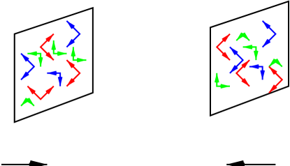
Figure 23: The collision of two sheets of colored glass.

represented as that of two sheets of colored glass. Before the collisions, the left moving hadron has fields

$$F^{i+} \sim \delta(x^{-})$$

$$F^{ij} \sim 0$$

$$F^{i-} \sim 0$$ (30)

and that of the right moving fields is analogous to that of the above save that $\pm\rightarrow\mp$ in the indices and coordinates of all fields. The fields are of course different in each nucleus. We shall consider impact parameter zero head on collisions in what follows.

These fields are plane polarized and have random colors. A solution of the classical Yang-Mill’s equation can be constructed by requiring that the fields are two dimensional gauge transforms of vacuum everywhere but in the forward light cone. At the edges of the light cone, and at its tip $t=z=0$, the equations are singular, and a global solution requires that the fields carry non-trivial energy and momentum in the forward lightcone. At short times, these fields are highly non-linear. In a time of order $\tau\sim 1/Q_{sat}$, the fields linearize. When they linearize, we can identify the particle content of the classical radiation field.

This situation is much different than the case for quantum electrodynamics. Because of the gluon self-interaction, it is possible to classically convert the energy in the incident nuclei into radiation. In quantum electrodynamics, the charged particles are fermions, and they cannot be treated classically. Radiation is produced by annihilation or bremstrahlung as quantum corrections to the initial value problem.

The solution to the field equation in the forward lightcone is approximately boost invariant over an interval of rapidity of order $\Delta y\ll 1/\alpha_{s}$. At large momentum, the field equations can be solved in perturbation theory and the distribution is like that of a bremstrahlung spectrum

$${{dN}\over{dyd^{2}p_{T}}}\sim{1\over\alpha_{s}}\pi R^{2}{Q_{sat}^{4}\over p_{T}^{4}}$$ (32)

It can be shown that such a spectrum matches smoothly onto the result for high momentum transfer jet production.

One of the outstanding problems of particle production is computing the total multiplicity of produced gluons. In the CGC description, this problem is solved. When $p_{T}\leq Q_{sat}$, non-linearities of the field equations become important, and the field stops going as $1/p_{T}^{4}$. Instead it becomes of order

$${{dN}\over{dyd^{2}p_{T}}}\sim{1\over\alpha_{s}}\pi R^{2}$$ (33)

The total multiplicty is therefore of order

$$N\sim{1\over\alpha_{s}}~{}\pi R^{2}Q_{sat}^{2}$$ (34)

If $Q_{sat}^{2}\sim A^{1/3}$, then the total multiplicty goes as A, the high $p_{T}$ differential multiplicity goes as $A^{4/3}$, as we naively expect for hard processes since they should be incoherent , and the low momentum differential multiplicity goes as $A^{2/3}$, since these particles arise from the region where the hadrons are black disks and the emission should take place from the surface.

In Fig. 24, the various kinematic regions for production of gluons are shown.

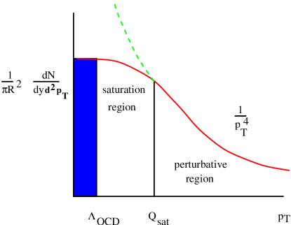
Figure 24: A cartoon representation of the various kinematic regions of gluon production.

In Fig. 25, the results of numerical simulation of gluon production are shown.

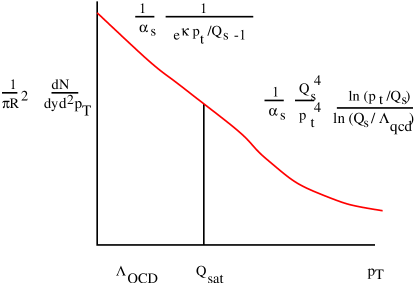
Figure 25: The numerically computed distribution of produced gluons.

At small $p_{T}$, it is amusing that the distribution is well described by a two dimensional Bose-Einstein distribution. This is presumably a numerical accident, and in this computation has absolutely nothing to do with thermalized distributions.

3.7 Thermalization

As shown in Fig. 17, in a heavy ion collision, the slow particles are produced first near the collision point and the slow particles are produced later far from the collision point. This introduces a gradiant into the initial matter distribution, and the typical comoving volume element expands like $1/\tau$. To understand the factor of $1/\tau$ in the above equation, note that if we convert $dN/dz=dN/dy~{}dy/dz=dN/dy~{}1/t$, where we used our previous definition of space-time rapidity, and where we evaluated at $z=0$. This is the physical rest frame density at $z=0$.

If entropy is conserved, as is the case for thermalized system with expansion time small compared to collision time,

$$S\sim T^{3}\tau R^{2}$$ (35)

is fixed so that $T\sim 1/\tau^{1/3}$. Therefore for a thermalized system, the energy density decreases as $\epsilon\sim 1/\tau^{4/3}$, where for system with no scattering so that the typical transverse momentum does not change, $\epsilon\sim 1/\tau$.

For the initial conditions typical of a Color Glass Condensate, thermalization is not so easy to do.[16] At the earliest times, the typical transverse momentum is large, of order of the saturation momentum. At this scale, the coupling is weak $\alpha_{s}(Q_{sat})<<1$, at least for asymptotically large energy.

To estimate the typical scattering time, we need to know the density and the mean free path. At early times, the density is that in the transverse space diluted by the longitudinal expansion of the system,

$$\rho=<p_{T}^{2}>/\tau$$ (36)

The scattering cross section is on the other hand $\sigma\sim\alpha^{2}_{s}ln(\rho)/<p_{T}^{2}>$. The logarithmic cutoff comes about from Debye screening the Coulomb cross section. (The linear divergence can be shown to cancel for thermalization processes.)

Thermalization requires that $\tau>>\tau_{scat}$, since $\tau$ itself is the characteristic expansion time. This requires that

$$\tau\geq exp(c/\alpha_{s})1/Q_{sat}$$ (37)

For practical purposes and for weakly coupled systems, there is never thermalization by elastic scattering!

Thermalization, if it in fact occurs, takes place by inelastic scattering. The physics of what is happening is easy to understand. Because the system begins its evolution with $p_{T}$ at such a large typical scale $Q_{sat}$, the coupling is weak and the system does not easily thermalize by elastic scattering. It therefore expands and becomes an overly dilute compared to the typical density associated with the transverse momentum scale $p_{T}^{3}$. When a system is overly dilute, the Debye screening length becomes very large. Multigluon production processes can be shown to diverge like the Debye screening length, whereas elastic processes only diverge like the logarithm of this length. Therefore, when the Debye screening length is of order $1/\alpha_{s}$, multigluon production begins to become more important than elastic scattering. This happens at a time $\tau\sim 1/(\alpha_{s}Q_{sat})$.

The details of how this thermalization occurs have not been fully worked out in detail. Current estimates of the time of thermalization matter produced in heavy ion collisions at RHIC energies ranges from $.3\leq\tau\leq 3~{}Fm/c$.

4 Lecture 3: What We Have Learned from RHIC

In this lecture, I review results from RHIC and describe what we have so far learned about the production of new forms of matter in heavy ion collisions. I will make the case that we have produced matter of extremely high energy density, so high that it is silly not to think of it as composed of quarks and gluons. I also will argue that this matter is strongly interacting with itself. The issue of the properties of this matter is still largely unresolved. For example whether the various quantities measured are more properly described as arising from a Color Glass Condensate or from a Quark Gluon Plasma, although we can easily understand in most cases which form of matter should be most important.

4.1 The Energy Density is Big

The particle multiplicity as a function of energy has been measured at RHIC, as shown in Fig. 26.

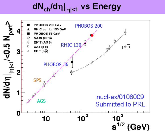
Figure 26: The particle multiplicity as a function of energy as has been measured at RHIC.

Combining the multiplicity data together with the measurements of transverse energy or of typical particle transverse momenta, one can determine the energy density of the matter when it decouples.[17] One can then extrapolate backwards in time. We extrapolate backwards using 1 dimensional expansion, since decoupling occurs when the matter first begins to expands three dimensionally. We can extrapolate backwards until the matter has melted from a Color Glass.

To do this extrapolation we use that the density of particles falls as $N/V\sim 1/t$ during 1 dimensional expansion. If the particles expand without interaction, then the energy per particle is constant. If the particles thermalize, then $E/N\sim T$, and since $N/V\sim T^{3}$ for a massless gas, the temperature falls as $T\sim t^{-1/3}$. For a gas which is not quite massless, the temperature falls somewhere in the range $T_{o}>T>T_{o}(t_{o}/t)^{1/3}$, that is the temperature is bracketed by the value corresponding to no interaction and to that of a massless relativistic gas. This 1 dimensional expansion continues until the system begins to feel the effects of finite size in the transverse direction, and then rapidly cools through three dimensional expansion. Very close to when three dimensional expansion begins, the system decouples and particles free stream without further interaction to detectors.

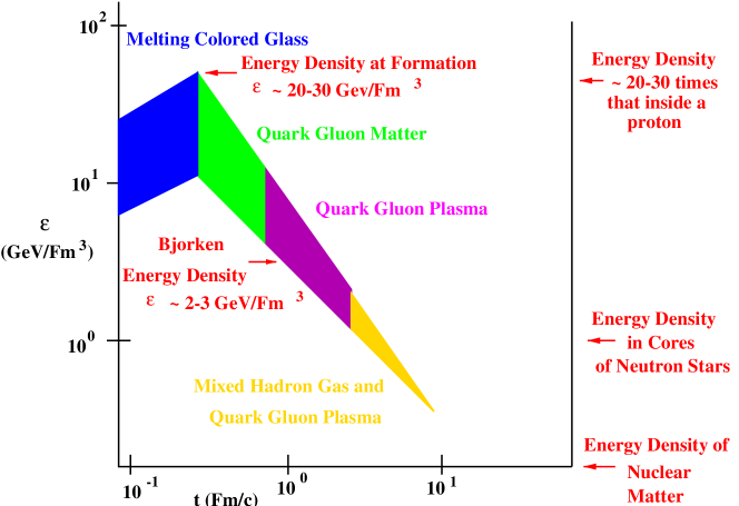
Figure 27: Bounds on the energy density as a function of time in heavy ion collisions.

We shall take a conservative overestimate of this time to be of order $t_{melt}\sim.3~{}Fm/c$ The extrapolation backwards is bounded by $\epsilon_{f}(t_{f}/t)<\epsilon(t)<\epsilon_{f}(t_{f}/t)^{4/3}$. The lower bound is that assuming that the particles do not thermalize and their typical energy is frozen. The upper bound assumes that the system thermalizes as an ideal massless gas. We argued above that the true result is somewhere in between. When the time is as small as the melting time, then the energy density begins to decrease as time is further decreased.

This bound on the energy density is shown in Fig. 27. On the left axis is the energy density and on the bottom axis is time. The system begins as a Color Glass Condensate, then melts to Quark Gluon Matter which eventually thermalizes to a Quark Gluon Plasma. At a time of a few $Fm/c$, the plasma becomes a mixture of quarks, gluons and hadrons which expand together.

At a time of about $10~{}Fm/c$, the system falls apart and decouples. At a time of $t\sim 1~{}Fm/c$, the estimate we make is identical to the Bjorken energy density estimate, and this provides a lower bound on the energy density achieved in the collision. (All estimates agree that by a time of order $1~{}Fm/c$, matter has been formed.) The upper bound corresponds to assuming that the system expands as a massless thermal gas from a melting time of $.3~{}Fm/c$. (If the time was reduced, the upper bound would be increased yet further.) The bounds on the energy density are therefore

$$2-3~{}GeV/Fm^{3}<\epsilon<20-30~{}GeV/Fm^{3}$$ (38)

where we included a greater range of uncertainty in the upper limit because of the uncertainty associated with the formation time. The energy density of nuclear matter is about $0.15~{}GeV/Fm^{3}$, and even the lowest energy densities in these collisions is in excess of this. At late times, the energy density is about that of the cores of neutron stars, $\epsilon\sim 1~{}GeV/Fm^{3}$.

At such extremely high energy densities, it is silly to try to describe the matter in terms of anything but its quark and gluon degrees of freedom.

4.2 The Gross Features of Multiplicity Distributions Are Consistent with Colored Glass

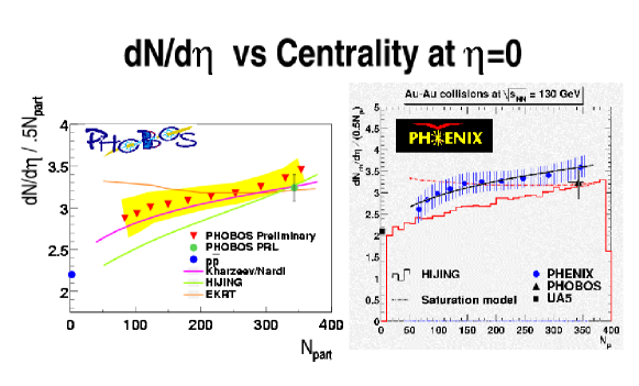
Figure 28: The CGC description of the participant dependence of the multiplicity of produced particles.

 

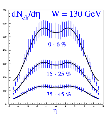
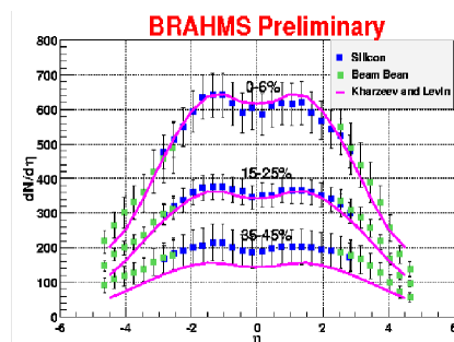
Figure 29: Color glass condensate fits to the rapidity density measured in the PHOBOS and Brahms experiments

As argued by Kharzeev and Nardi,[18] the density of produced particles per nucleon which participates in the collision, $N_{part}$, should be proportional to $1/\alpha_{s}(Q_{sat})$, and $Q_{sat}^{2}\sim N_{part}$. This dependence follows from the $1/\alpha_{s}$ which characterizes the density of the Color Glass Condensate. In Fig. 28, we show the data from PHENIX and PHOBOS[19]. The Kharzeev-Nardi form fits the data well. Other attempts such as HIJING[20], or the so called saturation model of Eskola-Kajantie-Ruuskanen-Tuominen[21] are also shown in the figure.

Kharzeev and Levin have recently argued that the rapidity distributions as a function of centrality can be computed from the Color Glass description.[22] This is shown in Fig. 29.[23]

4.3 Matter Has Been Produced which Interacts Strongly with Itself

In off zero impact parameter heavy ion collisions, the matter which overlaps has an asymmetry in density relative to the reaction plane. This is shown in the left hand side of Fig. 30. Here the reaction plane is along the x axis. In the region of overlap there is an $x-y$ asymmetry in the density of matter which overlaps. This means that there will be an asymmetry in the spatial gradients which will eventually transmute itself into an asymmetry in the momentum space distribution of particles, as shown in the right hand side of Fig. 30.

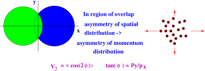
Figure 30: The asymmetry in the distribution of matter in an off center collision is converted to an asymmetry of the momentum space distribution.

This asymmetry is called elliptic flow and is quantified by the variable $v_{2}$. In all attempts to theoretically describe this effect, one needs very strong interactions among the quarks and gluons at very early times in the collision.[24]. In Fig. 31, two different theoretical descriptions are fit to the data by STAR and PHOBOS[25]-[26]. On the left hand side, a hydrodynamical model is used.[27] It is roughly of the correct order of magnitude and has roughly the correct shape to fit the data. This was not the case at lower energy. On the right hand side are preliminary fits assuming Color Glass.[28] Again it has roughly the correct shape and magnitude to describe the data. In the Color Glass, the interactions are very strong essentially from $t=0$, but unlike the hydrodynamic models it is field pressure rather than particle pressure which converts the spatial anisotropy into a momentum space-anisotropy.

Probably the correct story for describing flow is complicated and will involve both the Quark Gluon Plasma and the Color Glass Condensate. Either description requires that matter be produced in the collisions and that it interacts strongly with itself. In the limit of single scatterings for the partons in the two nuclei, no flow is generated.

 

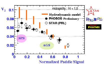
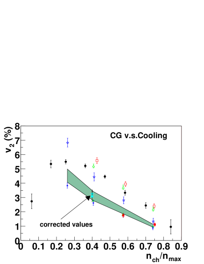
Figure 31: a) A hydrodynamic fit to v2. b) The Colored Glass fit.

4.4 What Do We Expect to Learn?

4.4.1 Does the Matter Equilibrate?

One of the most interesting results from the RHIC experiments is the so called “jet quenching”.[29]-[30]. In Fig. 32a, the single particle hadron spectrum is scaled by the same result in $pp$ collisions and scaled by the number of

 

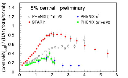
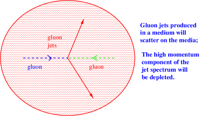
Figure 32: a) The $p_{T}$ distribution of particles scaled by the data from $pp$ collisions times the number of hard collisions inside the nuclei. b) A pair of jets is produced in a hard collision and they propagate through the surrounding matter.

collisions. The number of collisions is the number of nucleon-nucleon interactions, which for central collisions should be almost all of the nucleons. One is assuming hard scattering in computing this number, so that a single nucleon can hard scatter a number of times as it penetrates the other nucleus. The striking feature of this plot is that the ratio does not approach one at large $p_{T}$. This would be the value if these particles arose from hard scattering which produced jets of quarks and gluons, and the jets subsequently decayed.

The popular explanation for this is shown in Fig. 32b. Here a pair of jets is produced in a gluon-gluon collision. The jets are immersed in a Quark Gluon Plasma, and rescatter as they poke through the plasma. This shifts the transverse momentum spectrum down, and the ratio to $pp$ collisions, where there is no significant surrounding media, is reduced.

The data, however suggestive, need to be improved before strong conclusions are drawn. For example, there are large systematic uncertainties in the $pp$ data which was measured in different detectors and extrapolated to RHIC energy. This will be resolved by measuring $pp$ collisions at RHIC. There is in addition some significant uncertainty in the AA data which becomes smaller in the ratio to $pp$ data when the data is measured in the same detector. There are nuclear modifications of the gluon distribution function, an effect which can be determined by measurements on $pA$ at RHIC. The maximum transverse momentum is limited by the event sample size, and the size will be greatly improved with this years run due to the higher luminosity and longer run time.

(After these lectures were given, results were presented from the dA experiments at RHIC. The experimenters claim that the initial state effects are disfavored as an explanation for the jet quenching seen in the Au-Au collisions. For a summary of their conclusions, please look at the power point presentations on the RHIC homepage, or the submitted papers.[31] It is the authors opinion that much more needs be done before this conclusions can be firmly established.)

One of the reasons why jet quenching is so important for the RHIC program is that it gives a good measure of the degree of thermalization in the collisions. If jets are strongly quenched by transverse momenta of $4~{}GeV$, then because cross sections go like $1/E^{2}$ for quarks and gluons, this would be strong evidence for thermalization at the lower energies typical of the emitted particles.

One can look for evidence of thermalization directly from the measured $p_{T}$ distributions. Here one can do a hydrodynamic computation and in so far as it agrees with the results, one is encouraged to believe that there is thermalization. On the other hand, these distributions may have their origin in the initial conditions for the collision, the Colored Glass. In reality, one will have to understand the tradeoff between both effects. The hydrodynamic models do a good job in describing the data for $p_{T}\leq 2~{}GeV$, Here there is approximate $m_{T}$ scaling, a characteristic feature of hydrodynamic computations. This scaling arises naturally because in hydrodynamic distribution are produced by flowing matter which has a characteristic transverse flow velocity with a well defined local temperature. Particles with the same $m_{T}$ should have arisen from regions with the same transverse flow velocity and temperature.

Hydrodynamical models successfully describe the data on $m_{T}$distributions.[32] In Fig. 33

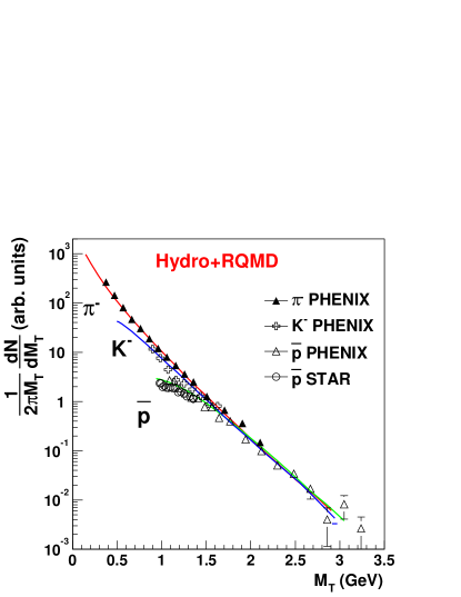
Figure 33: The hydrodynamical model fits to the $m_{T}$ spectra for the PHENIX and STAR data.

the results of the simulation by Shuryak and Teaney are shown compared to the STAR and PHENIX data.[29]-[30] The shape of the curve is a prediction of the hydrodynamic model, and is parameterized somewhat by the nature of the equation of state. Notice that the STAR data include protons near threshold, and here the $m_{T}$ scaling breaks down. The hydrodynamic fits get this dependence correctly, and this is one of the best tests of this description. The hydrodynamic models do less well on fits to the more peripheral collisions. In general, a good place to test the hydrodynamic models predictions is with massive particles close to threshold, since here one deviates in a computable way from the $m_{T}$ scaling curve, which is arguably determined from parameterizing the equation of state.

If one can successfully argue that there is thermalization in the RHIC collisions, then the hydrodynamic computations become compelling. One should remember that hydrodynamics requires an equation of state plus initial conditions, and these initial conditions are determined by Colored Glass. Presumably, a correct description will require the inclusion of both types of effects.[33]

4.4.2 Confinement and Chiral Symmetry Restoration

We would like to know whether or not deconfinement has occurred in dense matter or whether chiral symmetry restoration has changed particle masses.

Figure 34: The CERES data on low mass electron-positron pairs. The expected contribution from ordinary hadrons is shown by the solid line. The data points are for the measured electron-positron pairs.

This can be studied in principle by measuring the spectrum of dileptons emitted from the heavy ion collision. These particles probe the interior of the hot matter since electromagnetically interacting particles are not significantly attenuated by the hadronic matter. For electron-positron pairs, the mass distribution has been measured in the CERES experiment at CERN[34], and is shown in Fig. 34. Shown in the plot is the distribution predicted from extrapolating from $pA$ collisions. There should be a clear $\rho$ and $\phi$ peak, which has disappeared. This has been interpreted as a resonance mass shift,[35], enhanced $\eta^{\prime}$ production, [36] but is most probably collisional broadening of the resonances in the matter produced in the collisions.[37] Nevertheless, if one makes a plot such as this and the energy density is very high and there are no resonances at all, then this would be strong evidence that the matter is not hadronic, i. e. the hadrons have melted.

The resolution in the CERES experiment is unpleasantly large, making it difficult to unambiguously interpret the result. Whether or not such an experiment could be successfully run at RHIC, much less whether the resolution could be improved, is the subject of much internal debate among the RHIC experimentalists.

4.4.3 Confinement and $J/\Psi$ Suppression

In Fig. 35, the NA(50) data for $J/\Psi$ production is shown.[38] In the first figure, the ratio of $J/\Psi$ production cross section to that of Drell-Yan is shown as a function of $E_{T}$, the transverse energy, for the lead-lead

 

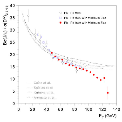
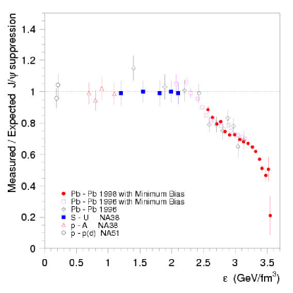
Figure 35: a) The ratio of produced $J/\Psi$ pairs to Drell-Yan pairs as a function of transverse energy $E_{T}$ at CERN energy. b) The measured compared to the theoretically expected $J/\Psi$ suppression as a function of the Bjorken energy density for various targets and projectiles.

collisions at CERN. There is a clear suppression at large $E_{T}$ which is greater than the hadronic absorption model calculations which are plotted with the data.[39] In the next figure, the theoretically expected $J/\Psi$ suppression based on hadronic absorption models is compared to that measured as a function of the Bjorken energy density for various targets and projectiles. There appears to be a sharp increase in the amount of suppression for central lead-lead collisions.

Is this suppression due to Debye screening of the confinement potential in a high density Quark Gluon Plasma?[40]-[42] Might it be due higher twists, enhanced rescattering, or changes in the gluon distribution function?[43]-[44] Might the $J/\psi$ suppression be changed into an enhancement at RHIC energies and result from the recombination in the produced charm particles, many more of which are produced at RHIC energy?[45]-[48]

These various descriptions can be tested by using the capability at RHIC to do $pp$ and $pA$ as well as $AA$. Issues related to multiple scattering, higher twist effects, and changes in the gluon distribution function can be explored. A direct measurement of open charm will be important if final state recombination of the produced open charm makes a significant amount of $J/\Psi$’s.

4.4.4 The Lifetime and Size of the Matter Produced

The measurement of correlated pion pairs, the so called HBT pion interferometry, can measure properties of the space-time volume from which the hadronic matter emerges in heavy ion collisions.[49] The quantities $R_{long},R_{side}$ and $R_{out}$ shown in Fig. 36 measure the transverse size of the matter at decoupling and the decoupling time.

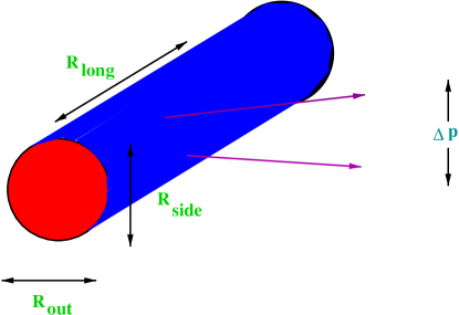
Figure 36: The various radii used for HBT pion interferometry.

 

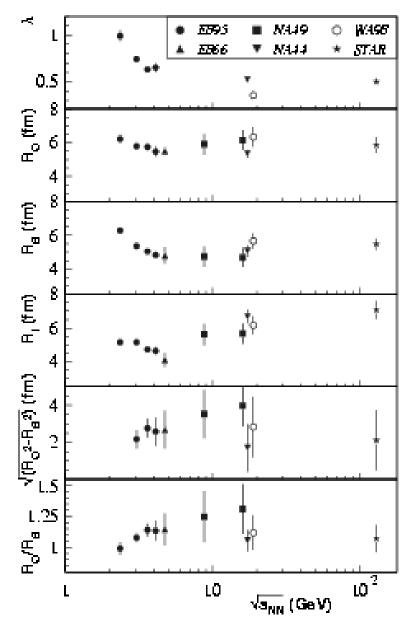
Figure 37: a) The various HBT radii measured in heavy ion experiments including the new data from STAR. b) The correlation functions which determine the radii as a function of the pair momenta measured in PHENIX.

In Fig. 37, the data from STAR and PHENIX is shown.[50]-[51] There is only a weak dependence on energy, and the results seem to be more or less what was observed at CERN energies. This is a surprise, since a longer time for decoupling is expected at RHIC. Perhaps the most surprising result is that $R_{out}/R_{side}$ is close to 1, where most theoretical expectations give a value of about $R_{out}/R_{side}\sim 2$.[52]-[53] Perhaps this is due to greater than expected opacity of the emitting matter? At this time, there is no consistent theoretical description of the HBT data at RHIC. Is there something missing in our space-time picture?

4.4.5 The Flavor Composition of the Quark Gluon Plasma

The first signal proposed for the existence of a Quark Gluon Plasma in heavy ion collisions was enhanced strangeness production.[54] This has lead to a comprehensive program in heavy ion collisions to measure

 

Figure 38: a) Various ratios of particle abundances and the RHIC data. The lines are the predictions of a thermal model. b) The temperature vs baryon chemical potential for a thermal model which is fit to data at various energies. The dashed line is a hypothetical phase boundary between a Quark Gluon Plasma and a hadronic gas.

the ratios of abundances of various flavors of particles.[55]. In Fig. 38a, the ratios of flavor abundances is compared to a thermal model for the particle abundances.[56] - [58] The fit is quite good. In Fig. 38b, the temperature and baryon chemical potential extracted from these fits is shown for experiments at various energies and with various types of nuclei. It seems to agree reasonably well with what might be expected for a phase boundary between hadronic matter and a Quark Gluon Plasma.

This would appear to be a compelling case for the production of a Quark Gluon Plasma. The problem is that the fits done for heavy ions to particle abundances work even better in $e^{+}e^{-}$ collisions. One definitely expects no Quark Gluon Plasma in $e^{+}e^{-}$ collisions. There is a deep theoretical question to be understood here: How can thermal models work so well for non-thermal systems? Is there some simple saturation of phase space? The thermal model description can eventually be made compelling for heavy ion collisions once the degree of thermalization in these collisions is understood.

5 Lecture 4: The Physics of the Color Glass Condensate

In this lecture, I discuss some of the implications of the Color Glass Condensate. I begin by developing in a little more detail the solutions for the fields of the Color Glass Condensate for a single hadron. I then discuss issues related to unitarity for electromagnetic probes of hadrons. I later argue that Froissart bound saturation for the total cross section in hadron-hadron scattering also arises naturally in the context of the Color Glass Condensate. Next, I show that a new scale appears in the gluon structure function and which corresponds to a new kind of Geometrical Scaling of high energy deep inelastic scattering. This scaling implies that there is a form of matter intermediate between the highly coherent Color Glass Condensate and the incoherent parton densities of perturbative QCD. Finally, I discuss the renormalization group and its implications for the high energy limit.

5.1 Formal Development: Light Cone Quantization

In light cone coordinates, the initial value problem is formulated along the surface $x^{+}=0$, and propagation is in terms of the light cone time $x^{+}$. This is shown in Fig. 39.

Figure 39: The initial value problem in lightcone coordinates. The light cone is shown and propagation from initial conditions at $x^{+}=0$ is shown.

Quantization of fields in light cone coordinates is most easily illustrated for the Klein-Gordon field. The equation of motion is

$$(p^{2}-M^{2})\phi=0$$ (39)

or

$$p^{-}\phi={{p_{T}^{2}+M^{2}}\over{2p^{+}}}\phi$$ (40)

Since $p^{-}=i\partial/\partial^{+}$, the first quantized Hamiltonian corresponding to this equation is

$$p^{-}={{p_{T}^{2}+M^{2}}\over{2p^{+}}}$$ (41)

To second quantize this system, we consider the action

$$S=\int d^{4}x{1\over 2}\left((\partial\phi)^{2}-M^{2}\phi^{2}\right)$$ (42)

The canonical momentum is

$$\Pi(x^{-},x_{T})={{\delta S}\over{\delta\partial_{+}\phi}}=\partial^{+}\phi={\partial\over{\partial x^{-}}}\phi$$ (43)

Note that the momentum $\Pi$ is on the same equal time surface as is $\phi$, and therefore it is not a variable independent of $\phi$. The momentum and coordinate are constrained, and therefore the quantization is subtle.

If we postulate the equal-time commutation relations

$$[\Pi(x^{-},x_{T}),\phi(y^{-},y_{T})]={{-i}\over 2}~{}\delta^{(3)}(x-y)$$ (44)

we see that

$$\partial_{-}^{x}[\phi(x),\phi(y)]={{-i}\over 2}\delta^{(3)}(x-y)$$ (45)

or that

$$[\phi(x),\phi(y)]={{-i}\over 2}~{}\epsilon(x^{-}-y^{-})\delta^{(2)}(x_{T}-y_{T})$$ (46)

One can check that these commutation relations generate the correct equations of motion for the action above. This leads to the creation and annihilation operator basis for the field $\phi$ of

$$\phi(x)=\int{{d^{3}p}\over{(2\pi)^{3}2p^{+}}}\theta(p^{+})\left(e^{-ipx}a(p)+e^{ipx}a^{\dagger}(p)\right)$$ (47)

where

$$[a^{b}_{i}(p),a^{c}_{j}(q)]=2p^{+}\delta^{bc}\delta_{ij}\delta^{(3)}(p-q)$$ (48)

Note that on the light one, only positive $p^{+}$ particles propagate. The vacuum has zero $p^{+}$, and since momentum is conserved, is trivial and has no particles in it. (This is true for the vacuum built to any order in perturbation theory. In fact the light cone limit is very subtle, and when one is careful to properly treat modes that have $p^{+}=0$, these modes can generate non-perturbative condensates for the vacuum.)

To quantize QCD, we work in light cone gauge, $A^{+}_{a}=0$. The equation of motion

$$D_{\mu}F^{\mu+}=-D_{i}F^{i+}+D^{+}F^{-+}=0$$ (49)

so that

$$A^{-}={1\over\partial^{+2}}D^{i}\partial^{+}A^{i}$$ (50)

The transverse degrees of freedom are quantized as

$$A^{i}_{a}=\int{{d^{3}p}\over{(2\pi)^{3}2p^{+}}}\left(e^{-ipx}a^{a}_{i}(p)+e^{ipx}a_{i}^{a\dagger}(p)\right)$$ (51)

If we want to compute the gluon content of the hadron, we compute

$${{2p^{+}}\over{(2\pi)^{3}}}=<h\mid a^{\dagger}(p)a(p)\mid h>={{2p^{+}}\over{(2\pi)^{3}}}<h\mid A^{ia}(p)A_{ia}(p)\mid h>$$ (52)

which we recognize as $2p^{+}/(2\pi)^{3}$ times the propagator $G^{ii}_{aa}(p,p;x^{+}-y^{+}\rightarrow 0)$

5.2 Formal Development: Solving the McLerran-Venugopalan Model

The McLerran-Venugopalan (MV) model involves the computation of the classical fields due to a lightcone current, and then averaging with a Gaussian weight over the external current strength. It is the simplest model with the physics of saturation built in. Instead of working in light cone gauge, it is simplest to first solve the classical equations of motion in the gauge $A^{-}=0$, and then to gauge rotate the result back to lightcone gauge. (The action for a Gaussian source can be written in a gauge invariant way because all values of the sources are integrated over with a gauge invariant measure.)

The equations of motion in $\overline{A}^{-}=0$ gauge are

$$D_{\mu}F^{\mu\nu}=\delta^{\nu+}\rho(x^{-},x_{T})$$ (53)

(We overline fields to indicate these are the fields in this gauge which must be rotated back to the light cone gauge. Fields in the light cone gauge will not be overlined.) These equations can be solved by the fields

$$\overline{A}^{i}=0$$ (54)

and

$$-\nabla^{2}_{T}\overline{A}^{+}=\overline{\rho}$$ (55)

Note that

$$\overline{\rho}=U^{\dagger}\rho U$$ (56)

where $U$ is the gauge rotation between this gauge and light cone gauge.

Since

$$\overline{A}^{\mu}=U^{\dagger}A^{\mu}U+{i\over g}U^{\dagger}\partial^{\mu}U$$ (57)

we have that

$$\overline{A}^{+}={i\over g}U^{\dagger}(\partial^{+}U)$$ (58)

Upon defining

$$\alpha=\overline{A}^{+}={1\over{-\nabla_{T}^{2}}}\overline{\rho}$$ (59)

we see that we can explicitly determine

$$U^{\dagger}(x)=Pexp\left(ig\int_{-\infty}^{x^{-}}dz^{-}\alpha(z^{-},x_{T})\right)$$ (60)

The fields in $A^{+}=0$ gauge are therefore

$$A^{+}=A^{-}=0$$ (61)

and

$$A^{i}={i\over g}U\nabla^{i}U^{\dagger}$$ (62)

If we choose $x^{-}$ to be outside the range of support of $\rho$, then these fields are of the simple form

$$A^{i}=\theta(x^{-})V\nabla^{i}V^{\dagger}$$ (63)

where

$$V^{\dagger}(x)=Pexp\left(ig\int_{-\infty}^{\infty}dz^{-}\alpha(z^{-},x_{T})\right)$$ (64)

5.3 The Gluon Distribution Function in the MV Model

We can now use the classical fields we determined above to compute the gluon distributions function. We have that

$${{dN}\over{d^{3}k}}={{2k^{+}}\over{(2\pi)^{3}}}<A^{i}_{a}(k,x^{+})A^{i}_{a}(-k,x^{+})>$$ (65)

where the $<O>$ notation means to average $O$ over all values of sources with a Gaussian weight. This averaging is straightforward to do for the gluon distribution function with the result that [15] (in coordinate space for both $x^{-}$ and $y^{-}$ greater than zero)

$$<A^{i}_{a}(x)A^{i}_{a}(y)>={{N_{c}^{2}-1}\over{\pi\alpha N_{c}}}{{1-e^{-x_{T}^{2}Q_{s}^{2}ln(x_{T}^{2}\Lambda^{2}_{QCD})/4}}\over x_{T}^{2}}$$ (66)

The saturation momentum is [59]-[60]

$$Q_{s}^{2}=2\pi N_{c}\alpha_{s}^{2}\int dx^{-}\mu^{2}(x^{-})\sim\alpha_{s}^{2}{{Charge^{2}}\over{area\times(N_{c}^{2}-1)}}$$ (67)

This equation is true only for $x_{T}<<1/\Lambda_{QCD}$, and also assumes that the scale of charge neutralization is the confinement scale. This neutralization scale becomes modified to $Q_{s}$ in a more first principles computation and the structure of the distribution function is modified for $1/\Lambda_{QCD}\geq x_{T}\geq 1/Q_{s}$. Note that the integral over $x^{-}$ in the definition of the saturation momentum can be converted to an integral over space time rapidity and that the charge being computes is the total at all rapidities greater than that of the scale of interest. One can use the DGLAP evolution equations to relate this directly to the gluon density.

The gluon distribution can now be computed in momentum space using the above formulae. One finds that at large $p_{T}$, it goes as $Q_{s}^{2}/\alpha_{s}p_{T}^{2}$, and at small $p_{T}$, it goes as $ln(Q_{s}^{2}/p_{T}^{2})/\alpha_{s}$. The gluon distribution is shown in Fig. 40

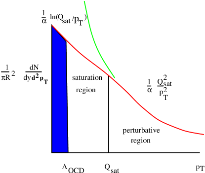
Figure 40: The gluon distribution function as computed in the Mclerran-Venugopalan model.

Note that the omnipresent factor of $1/\alpha_{s}$ arises from the strong gluon fields and is typical of condensation phenomena.

At large $p_{T}$, the behaviour as $Q_{s}^{2}/p_{T}$2 is typical of bremstrahlung from a number of independent sources characterized by the gluon distribution function. At small $p_{T}$, these sources add together coherently, and the monopole nature of the fields strength is canceled. This is because at these $p_{T}$ scales, the typical separation between sources is less than the scale at which the field is measured.

We expect that the saturation momentum will grow quickly with $1/x$, perhaps a power of $1/x$. The tail of the distribution in $p_{T}$ therefore grows rapidly with $1/x$, but below $Q_{s}$, the distribution is slowly varying. This behaviour solves the unitarity problem associated with the energy dependence of distribution functions. If we measure the number of gluon below some resolution scale $Q^{2}$,

$$xG(x,Q^{2})\sim\int_{0}^{Q^{2}}d^{2}p_{T}{{dN}\over{d^{2}p_{T}dy}}$$ (68)

this goes as $\pi R^{2}Q^{2}$ for $Q\leq Q_{s}$ and $\pi R^{2}Q_{s}^{2}$ for $Q\geq Q_{s}$. So at fixed Q at very small x, it will always be true that $Q\leq Q_{s}$ and cross sections will grow geometrically. In the MV model, $Q_{s}^{2}\sim R$, and therefore at large $Q\geq Q_{s}$, the cross section grows rapidly and scales as the volume of the system. (In fact at very small x it turns out that the renormalization group equations give a $Q_{s}$ independent of $R$, although there is still a rapid increase with energy.)

5.4 Hadronic Cross Sections and Froissart Bound Saturation

The Froissart bound is that a total hadronic cross section must satisfy [8]-[9]

$$\sigma\leq Cons\times ln^{2}(E)$$ (69)

at high energy $E$. This may be simply understood in the language of the Color Glass Condensate.[10]-[11] Suppose that the saturation momentum grows like an exponential in rapidity at small x $y\sim ln(1/x)$. let us also assume that the saturation momentum is a function of rapidity and that it factorizes into an impact parameter dependent piece and a $y$ dependent piece,

$$Q_{s}^{2}(y,b)=Q_{s}^{2}(y,0)F(b)$$ (70)

Let us assume that

$$Q_{s}^{2}(y,0)\sim e^{\kappa y}$$ (71)

At large $b$, we expect that $F(b)\sim e^{-2m_{\pi}b}$, since an isosinglet quantity like the gluon distribution function’s large distance effect should be controlled by two pion exchange.

Now if we measure a cross section at some value of $Q^{2}$, then it better be true that the target becomes dark at an impact parameter which satisfies

$$Q^{2}=Q^{2}_{s}(y,b)$$ (72)

or that the impact parameter where this occurs satisfies

$$b\sim\kappa y/2m_{\pi}$$ (73)

Therefore the cross section saturates the Froissart bound

$$\sigma\sim y^{2}$$ (74)

To fill in the details of this argument involves much work and the interested student is invited to explore the literature where these issues are discussed, and are continuing to be argued, in the literature.

5.5 Geometrical Scaling

Geometric scaling is the condition that the structure functions for quarks and gluons are functions only of the dimensionless ration $Q^{2}/Q_{s}^{2}$, up to an overall factor which carries the overall dimension.[61]-[65] For deep inelastic scattering, it is the requirement

$$\sigma_{\gamma^{*}p}\sim F_{2}(x,Q^{2})/Q^{2}\sim G(Q^{2}/Q_{s}^{2})$$ (75)

This condition is obvious when $Q^{2}<<Q_{s}^{2}$, but a surprising result is that it is also true up to $Q^{2}\leq Q_{s}^{4}/\Lambda^{2}_{QCD}$. This weaker bound can take one to quite high values of $Q^{2}$ at small values of $x$.

The worlds data at $x\leq 10^{-2}$ is shown in Fig. 41 as a function of $\tau=Q^{2}/Q_{s}^{2}$

Figure 41: $\sigma_{\gamma^{*}p}$ as a function of the scaling variable $\tau=Q^{2}/Q_{s}^{2}$.

It seems to scale in terms of the saturation momentum.

To understand how geometrical scaling can arise, consider the simple example of the unintegrated gluon distribution function in the double logarithm approximation. Here

$$F(x,Q^{2})=\Lambda^{2}_{QCD}e^{\sqrt{Aln(1/x)ln(Q^{2}/\Lambda_{QCD}^{2})}}$$ (76)

The gluon distribution function is the number of gluons per unit area with momentum less than $Q^{2}$. When $Q^{2}\sim Q_{sat}^{2}$, this density is of the order of $Q_{sat}^{2}$, as we saw in previous sections. This gives us an equation for the saturation momentum

$$Q_{sat}^{2}=\Lambda_{QCD}^{2}e^{Aln(1/x)}$$ (77)

This predicts a power law dependence upon the $x$ in agreement with phenomenology. This has a relatively large correction due to running the coupling constant, but in fact one can compute the saturation momentum’s dependence on $x$ in a systematic way and the result, remarkably, agrees with phenomenology.

Now if go back and express $\Lambda^{2}_{QCD}$ in terms of $Q_{sat}^{2}$, and require that $Q^{2}<<Q_{sat}^{4}/\Lambda^{2}_{QCD}$, we find that

$$F(x,Q^{2})\sim(Q^{2}/Q_{sat}^{2})^{1/2}$$ (78)

The gluon distribution function acquires an anomalous dimension of $1/2$. Again this can be done beyond the double logarithmic approximation, and one can find the above arguments go through save that the anomalous dimension is a little changed from $1/2$, and that the power law dependence of the saturation momentum is changed. The interested student is referred to the original literature to see this fully developed.

This result has the consequence that the effects of saturation extend far beyond the region of momentum where there is a Color Glass Condensate $Q^{2}\leq Q_{sat}^{2}$, into a new region $Q_{sat}^{2}\leq Q^{2}\leq Q_{sat}^{4}/\Lambda^{2}_{QCD}$. In this new extended scaling region, distribution functions have pure power law behaviour reminiscent of critical phenomena in condensed matter systems. This region has been called the Extended Scaling Region and sometime the Quantum Colored Fluid. A diagram which shows the various kinematic regions is shown in Fig. 42.

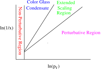
Figure 42: The kinematic regions in the $ln(1/x)-ln(Q^{2})$ plane which correspond to Extended Scaling and to the Color Glass Condensate

5.6 The Renormalization Group

The result of our considerations for an effective action for the Color Glass Condensate gave path integral representation of the form

$$\int[dA][d\rho]exp\left(iS[A,\rho]-F[\rho]\right)$$ (79)

In this equation $S$ is the action for the gluon fields in the presence of a light cone current described by the charge density $\rho$. (To define it properly one must provide a manifestly gauge invariant action.) Once one solves for the fields in terms of $\rho$, then one is required to average over the source with a weight function $F[\rho]$ which in the Mclerran-Venugopalan model is taken as a Gaussian. Implicit in the path integral is a longitudinal momentum cutoff. The fields have momenta below this cutoff, and the effect of integrating out the fields above the cutoff is included in the source $\rho$ and the integration over various values of $\rho$.

The question arises: How does one determine $F[\rho]$? It turns out that $F$ is determined by renormalization group equations generated by varying the longitudinal momentum cutoff.[14]-[15],[60], [66]-[68] The reason why the renormalization group treatment is essential follows from trying to solve for physical quantities, such as the gluon distribution function within the CGC approach. In lowest order one computes the classical field associated with the source $\rho$, inserts it into an expression for the operator of interest, and then averages over $\rho$. The lowest order corrections to this involve Gaussian fluctuations around this classical solution. If there is some scale associated with the process of physical interest, say $p^{+}$, one finds that the first order corrections are of order $\alpha_{s}ln(\Lambda^{+}/p^{+})$, where $\Lambda^{+}$ is the longitudinal momentum cutoff. The coupling constant $\alpha$ is small because we evaluate it at the saturation momentum scale. The quantum corrections to the lowest order result are therefore small so long as

$$e^{-c/\alpha_{s}}\Lambda^{+}<<p^{+}\leq\Lambda^{+}$$ (80)

In order to go to lower momenta, it is easiest to change the longitudinal momentum cutoff to a smaller value. To do this, we have to integrate out the degrees of freedom between the old longitudinal momentum cutoff scale and the new one. This can be done in Gaussian approximation since the coupling is weak, and so long as the ratio of the various cutoff scales satisfies $\alpha_{s}ln(\Lambda^{+}/\Lambda^{+\prime})<<1$. It turns out that this integration does not change the action for the interaction of the gluon fields with the source. All that changes is the weight function for integration over the source fields. If we let

$$dy=ln(\Lambda^{+}/\Lambda^{+\prime})$$ (81)

the renormalization group equation becomes

$${d\over{dy}}e^{-F[\rho]}=-H(\rho,d/d\rho)e^{-F[\rho]}$$ (82)

It turns out that $H$ is second order in $d/d\rho$, real, and positive semidefinite. Therefore $H$ can be interpreted as a Hamiltonian for a $2+1$ dimensional quantum system.

The Hamiltonian above has an unusual property. If there was a potential for the Hamiltonian $H$ with a unique minimum, then the at large times the solution of the above equation would tend towards the ground state. In the Color Glass Condensate $H$, there is in fact zero potential. The system never tends to the ground state, and there is quantum diffusion. To see how this works consider a 1 dimensional example.

$${d\over dy}Z={{-p^{2}}\over 2}Z$$ (83)

This has the solution

$$Z={1\over\sqrt{2\pi y}}exp\left(-x^{2}/2y\right)$$ (84)

As the Euclidean time $y$ increases, the wavefunction spreads, corresponding to diffusion. This is unlike the situation where there is a potential

$${d\over{dy}}Z=\left({{-p^{2}}\over 2}-V(x)\right)Z$$ (85)

Here as we evolve in time, the coordinate $x$ settles into the minimum of $V$, and has small excursions around it. The solution for $Z$ becomes time independent.

The consequences of this simple observation are enormous. For the case of diffusion, physical quantities are never independent of rapidity, even at the smallest values of $x$. The non-triviality of the small $x$ limit is a consequence of the lack of a potential in the renormalization group evolution equation!

The interested reader is referred to the growing literature on this subject for details. Suffice it to say that one can use the renormalization group equation above, and the explicit form for $H$ which has been computed to reproduce all known renormalization group equations. The explicit form of the equations exists, and various approximate solutions have been constructed. The picture which results agrees with the phenomenology of small x physics. Understanding and solving these equations provides a rich area for future research.

6 Acknowledgements

I grateful acknowledge conversations with Dima Kharzeev, Robert Pisarski and Raju Venugopalan on the subject of this talk. Much of the material in the first three lectures was also presented in the 2003 Moscow Winter School of Theoretical Physica and will be published in Surveys in High Energy Physics.

This manuscript has been authorized under Contract No. DE-AC02-98H10886 with the U. S. Department of Energy.

References

- [1] For a summary of recent results see the excellent review talk by Jean-Paul Blaizot, Lectures at the 40th Internationale Universitatswochen fuer Theoretische Physik: Dense Matter (IUKT 40), Schladming, Styria, Austria, 3-10 Mar 2001. Published in Lect.Notes Phys.583:117-160,2002 Also in *Schladming 2001, Lectures on quark matter* 117-160; hep-ph/0107131
- [2] For a state of the art up to date review on the properties of the Color Glass Condensate, see E. Iancu and R. Venugopalan, to be published in QGP3, R. C. Hwa and X. N. Wang, World Scientific; hep-ph/0303204
- [3] For a review about the prospects for spin physics at RHIC and other accelerators see G. Bunce, N. Saito, J. Soffer and W. Vogelsang, Ann. Rev. Part. Sci., 50, 525 (2000).
- [4] J. C. Collins and M. J. Perry, Phys. Rev. Lett. 34, 1353 (1975);
- [5] For a summary of recent results see the excellent review talk by F. Karsch, Lectures at the 40’th Internationale Universitatswochen fuer Theoretische Physik, Dense Matter, Schladming, Styria, Austria, 3-10 March 2001, published in Lect.Notes Phys.583:209-249,2002 Also in *Schladming 2001, Lectures on quark matter* 209-249; hep-lat/0106019.
- [6] L. V. Gribov, E. M. Levin and M. G. Ryskin, Phys. Rept. 100, 1 (1983); A. H. Mueller and Jian-wei Qiu, Nucl. Phys. B268, 427 (1986); J.-P. Blaizot and A. H. Mueller, Nucl. Phys. B289, 847 (1987); L. D. McLerran and R. Venugopalan, Phys. Rev. D49, 2233(1994); 3352 (1994); E. Iancu, A. Leonidov and L. D. McLerran, Nucl. Phys. A692(2001); E. Ferreiro E. Iancu, A. Leonidov and L. D. McLerran, hep-ph/0109115;
- [7] J. Breitweg et. al. Eur. Phys. J. 67, 609 (1999)
- [8] M. Froissart, Phys. Rev. 123 (1961) 1053.
- [9] A. Martin, Nuovo Cimento 42 (1966) 930; L. Lukaszuk and A. Martin, Nuovo Cimento 52 (1967) 122.
- [10] E. Ferreiro, E. Iancu, K. Itakura and L. McLerran, Nuc. Phys. A710, 373 (2002)
- [11] A. Kovner and U. Wiedemann, Phys. Rev. D66, 051502 (2002); Phys. Lett. B551, 311 (2003).
- [12] A. Kovner, L. D. McLerran and H. Weigert, Phys. Rev. D52, 6231 (1995); 3809 (1995); A. Krasnitz and R. Venugopalan, Phys. Rev. Lett 84, 4309 (2000); Nucl. Phys. B557, 237 (1999); A. Krasnitz, Y. Nara and R. Venugopalan, Phys. Rev. Lett. 87 , 192302 (2001).
- [13] B. B. Back et. al. nucl-ex/020015
- [14] J. Jalilian-Marian, A. Kovner, L. McLerran and H. Weigert, Phys. Rev. D55 (1997), 5414.
- [15] J. Jalilian-Marian, A. Kovner, A. Leonidov and H. Weigert, Nucl. Phys. B504 (1997), 415; Phys. Rev. D59 (1999), 014014.
- [16] R. Baier, A.H. Mueller, D. Schiff and D.T. Son, Phys. Lett. B502 (2001) 51.
- [17] B. B.Back et. al., Phys. Rev. Lett. 85, 3100 (2000);
- [18] D. Kharzeev, M. Nardi, Phys. Lett. B507 (2001) 121.
- [19] B. Back et. al. nucl-ex/0105011; K. Adcox et. al. Phys. Rev. Lett. 86, 3500 (2001).
- [20] M. Gyulassy and Xin-Nian Wang, Comput. Phys. Commun 83, 307 (1994).
- [21] K. Eskola, K. Kajantie, P. Ruuskanen and K. Tuominen, Nucl. Phys. B570, 379 (2000); K. Eskola, K. Kajantie and K. Tuominen, Phys. Lett. B497, 39 (2001)
- [22] D. Kharzeev and E. Levin, nucl-th/0108006.
- [23] B. Back et. al. Phys. Rev. Lett. 87, 102303 (2001); I. Beardon et. al. Nucl-ex/0112001.
- [24] S. Voloshin and Y. Zhang, Z. Phys. C70, 665 (1996); A. M. Poskhanzer and S. A. Voloshin, Phys. Rev. C58, 1671 (1998); J. Y. Ollitrault, Phys. Rev. D46, 229 (1992)
- [25] K, H. Ackermann et. al. Phys. Rev. Lett. 86, 402 (2001); C. Adler et. al. Phys. Rev. Lett. 87, 182301 (2001).
- [26] R. Lacey (for the PHENIX collaboration), Nucl. Phys. A698, 559 (2002)
- [27] Peter F. Kolb, J. Sollfrank, and U. Heinz, Phys. Lett. B459, 667 (1999); P. F. Kolb, P. Huovinen, U. Heinz and H. Heiselberg, Phys. Lett. B500, 232 (2001).
- [28] A. Krasnitz, Y. Nara and R. Venugopalan, in preparation.
- [29] C. Adler, Phys. Rev. Lett. 87 112303 (2001)
- [30] K. Adcox et. al. Phys. Rev. Lett 88, 022301 (2002).
- [31] I. Arsene et.al. nucl-ex/0307003; B. B. Back et. al. nucl-ex/0306025; S. S. Adler et. al. nucl-ex/0306021; J. Adams et. al. nucl-ex/0306024.
- [32] D. Teaney and E. V. Shuryak, Phys. Rev. Lett. 83, 4951 (1999): D. Teaney, J. Lauret and E. V. Shuryak, nucl-th/0110037
- [33] D. K. Srivastava, Phys. Rev. C64, 064901 (2001).
- [34] G. Agakishiev et. al. Nucl. Phys. A638, 159 (1998).
- [35] G. E. Brown and M. Rho, Phys. Rept., 269, 333 (1996).
- [36] J. Kapusta, D. Kharzeev, L. D. McLerran, Phys. Rev. D53, 5028 (1996).
- [37] R. Rapp, G. Chanfry and J. Wambach, Phys. Rev. Lett. 76, 368 (1996).
- [38] For the latest results, see M. C. Abreau et. al. Nucl. Phys. A661, 93 (1999).
- [39] J. Geiss, E. Bratskaya, W. Cassing and C. Greiner, nucl-th/981005,; C. Spieles, R. Vogt, L. Gerland, S. A. Bass, M. Bleicher, H. Stocker and W. Greiner, Phys. Rev. C60, 054901 (1999); D. E. Kahana and S. H. Kahana, Phys. Rev. C60, 065206 (1999); N. Armesto, A. Capella, E. Ferreiro, A. Kaidalov and D. Sousa, Nucl. Phys. A698, 583 (2002).
- [40] T. Matsui and H. Satz, Phys. Lett., bf B178, 416 (1986).
- [41] D. Kharzeev and H. Satz, Phys. Lett. B334, 155 (1994).
- [42] Jean-Paul Blaizot and Jean-Yves Ollitrault, Phys. Rev. Lett. 77, 1703 (1996).
- [43] J. Armesto and A. Capella, Phys. Lett. B430, 23 (1998); A. Capella, E. G. Ferreiro, A. Kaidalov, Phys. Rev. Lett. 85, 2080 (2000).
- [44] Jian-wei Qiu, James P. Vary and Xiao-fei Zhang, hep-ph/9809442.
- [45] R. Thews, M. Schroeder and J. Rafelski, Phys. Rev. C63, 054905 (2001).
- [46] P. Braun-Munzinger and J. Stachel, Phys. Lett. B490, 196 (2000).
- [47] P. Braun-Munzinger and K. Redlich, Eur. Phys. J. C16, 519 (2000).
- [48] M. Gorenstein and M. Gazdzicki, Phys. Rev. Lett. 83, 4009 (1999). M. Gorenstein, A. P. Kostyk, H. Stoecker and W. Greiner, Phys. Lett. B509, 277 (2001); M. Gorenstein, A. Kostyk, L. McLerran, H. Stoecker and W. Greiner, hep-ph/0012292; M. Gorenstein, A. Kostyk, H. Stocker and W. Greiner, Phys. Lett. B524, 265 (2002)
- [49] M. Gyulassy, S. Kauffmann and L. Wilson, Phys. Rev. C20, 2267 (1979).
- [50] C. Adler et. al. Phys. Rev. Lett. 87 , 082301 (2001).
- [51] K. Adcox et. al. nucl-es/0201008.
- [52] S. Chapman, P. Scotto and U. Heinz, Phys. Rev. Lett. 74, 4400 (1995); S. Chapman and U. Heinz, Phys. Lett B340, 250 (1994).
- [53] S. Soff, S. Bass and A. Dumitru, Phys. Rev. Lett. 86, 3981 (2001).
- [54] B. Muller and J. Rafelski, Phys. Rev. Lett. 48 1066 (1986); P. Koch, B. Muller and J. Rafelski, Phys. Rept. 142 167 (1986).
- [55] For a summary see: M. Kaneta and N. Xu, J. Phys. G27, 589 (2001).
- [56] For a state of the art assessment review, see Jean. Cleymans, hep-ph/0201142; J. Cleymans and K. Redlich, Phys. Rev. Lett. 81, 5284 (1998); Phys. Rev. C60, 054908 (1999).
- [57] P. Braun-Munzinger, J. Stachel, J. P. Wessels and N. Xu, Phys. Lett. B365, 1 (1996); P. Braun-Munzinger, I. Heppe and J. Stachel, Phys. Lett. B465, 15 (1999).
- [58] G. Yen and M. Gorenstein, Phys. Rev. C59, 2788 (1999).
- [59] A. H. Mueller, Nucl. Phys. B558 (1999), 285.
- [60] E. Iancu, A. Leonidov and L. McLerran, Nucl. Phys. A692 (2001) 583; Phys. Lett. B510 (2001) 133; E. Ferreiro, E. Iancu, A. Leonidov and L. McLerran, Nucl. Phys. A703 (2002) 489.
- [61] K. Golec-Biernat and M. Wüsthoff, Phys. Rev. D59 (1999), 014017; ibid. D60 (1999), 114023; Eur. Phys. J. C20 (2001) 313.
- [62] A. H. Mueller and D. N. Triantafyllopoulos, Nucl. Phys. B 640, 331 (2002).
- [63] D. N. Triantafyllopoulos, Nucl. Phys. B 648, 293 (2003).
- [64] A. M. Stasto, K. Golec-Biernat and J. Kwiecinski, Phys. Rev. Lett., 86, 596 (2001).
- [65] E. Iancu, K. Itakura and L. McLerran, Nucl. Phys. A 708, 327 (2002); arXiv:hep-ph/0205198.
- [66] I. Balitsky, Nucl. Phys. B463 (1996), 99; High-energy QCD and Wilson lines, hep-ph/0101042.
- [67] Yu. V. Kovchegov, Phys. Rev. D60 (1999), 034008; ibid. D61 (2000), 074018.
- [68] A. H. Mueller, Phys. Lett. B523 (2001) 243.